1. Introduction

A recurring problem in scientific computing is the simulation of the scattering of acoustic waves in media with variable wave speed, an environment which arises in a wide variety of applications such as seismology, ultrasound tomography, and sonar. We are specifically interested in a situation in time-harmonic scattering with wavenumber $\kappa>0$, where a given incident field $u^{\rm inc}$ impinges on a medium with smooth wave speed $v=v(\bm{x})$ that takes on a constant value $v_{\rm free}$ everywhere outside of a finite domain $\Omega$. The scattered field can then be written

(1) $$u(\bm{x})=\int_{\Omega}G(\bm{x},\bm{y})\sigma(\bm{y})\,d\bm{y},\quad x\in\mathbb{R}^{2},$$

where

(2) $$G(\bm{x},\bm{y})=\frac{i}{4}H_{0}(\kappa\|\bm{x}-\bm{y}\|).$$

The density $\sigma$ is unknown a priori and can be obtained by solving the Lippmann-Schwinger equation given by

(3) $$\sigma(\bm{x})+\kappa^{2}b(\bm{x})\int_{\Omega}G(\bm{x},\bm{y})\sigma(\bm{y})\,d\bm{y}=-\kappa^{2}b(\bm{x})u^{\rm inc}(\bm{x}),\quad\bm{x}\in\mathbb{R}^{2}.$$

The function $b$, which we refer to as a scattering potential, specifies how much the wave speed deviates from the free-space wave speed:

$$b(\bm{x})=1-\frac{v_{\rm free}^{2}}{v(\bm{x})^{2}}.$$

As long as $b$ is bounded above by 1, existence and uniqueness of the solution is guaranteed [8, Theorem 8.7].

The presence of the free-space fundamental solution in (1) makes the formulation immune to pollution error (cf. [2]) and guarantees that the scattered field will satisfy the Sommerfeld radiation condition, avoiding the need for special techniques, such as absorbing boundary conditions [11] or perfectly matched layers [3], which would be required if a differential equation formulation of the scattering problem were directly discretized. Moreover, (3) is typically a Fredholm equation of the second kind (for instance when viewed as an operator on $L^{2}(\Omega)$), which admits well-conditioned high-order accurate discretizations.

Remark 1.1.

The equation (3) is obtained by inserting (1) as an ansatz into the variable-coefficient Helmholtz equation

(4) $$-\Delta u^{\rm tot}(\bm{x})-\kappa^{2}(1-b(\bm{x}))u^{\rm tot}(\bm{x})=0,\quad\bm{x}\in\mathbb{R}^{2},$$

where $u^{\rm tot}=u^{\rm inc}+u$ is the total field, and then applying the fact that the incident field satisfies the homogeneous free-space Helmholtz equation.

Integral equation formulations of scattering problems do come with certain trade-offs. Particularly, they upon discretization lead to linear systems with dense coefficient matrices. Additionally, the fact that the kernel in (3) is singular necessitates some care in order to attain high-order accurate discretizations. Both of these issues were addressed in [10], where the authors present a high-order accurate quadrature rule that is tailored specifically for (3), and use an FFT to rapidly apply the global operator. (This is possible since the kernel $G(\bm{x},\bm{y})$ in (3) is translation invariant, and a regular square mesh is used for the discretization.) This allows for iterative solvers to be used, and the overall solver is shown to be highly effective in many environments. However, it turns out that as the wavenumber $\kappa$ grows, the iteration count required grows prohibitively, especially when the scatterer is highly refractive. This may seem surprising given that (3) is a second kind Fredholm equation, but it is explained by the fact that as $\kappa$ grows, the magnitude of the second term in (3) grows as $\kappa^{2}$, which means that it quickly comes to dominate the first term, and the overall behavior of the integral equation tends towards the behavior of a first kind equation.

To overcome the difficulties posed by the slow convergence of iterative methods for problems with oscillatory solutions, one may look to utilize a direct solver, leveraging the rank structure of the linear system. Many data-sparse matrix formats and corresponding inversion algorithms have been proposed, including $\mathcal{H}$- [17], $\mathcal{H}^{2}$- [4], Hierarchically Off-Diagonal Low Rank (HODLR) [1] and Hierarchically Block/Semi- Separable (HBS/HSS) matrices [21, 6, 26]. These format are differentiated by whether or not the interactions between adjacent patches in the domain are compressed and whether or not the basis matrices used in the hierarchical structure are taken to be nested [20, Sec. 15.8]. In this work, we rely on the so called HBS format, which uses nested bases ($\mathcal{H}^{2}$ rather than $\mathcal{H}$ structure), and does compress adjacent patches (“weak admissibility”). These ideas trace back to, e.g., [21, 22, 15, 24].

There are two general approaches to inverting HBS matrices. The first approach is to compute the factors of a data-sparse representation of the inverse through use of explicit formulas in terms of the factors of the original HBS matrix. The prototypical example of this is reviewed in [13]. Often, these can be viewed as derived through the recursive usage of variants of the Woodbury formula. Generally, such methods achieve high practical speed and are relatively memory efficient. The weakness of these methods is that they can run into stability issues if ill-conditioned matrices are encountered during the inversion process. This is especially prevalent for problems like the Lippmann-Schwinger equation where the off-diagonal blocks of the discretized system can vary drastically in magnitude due to the presence of the scattering potential. The second approach is to use rank structure to create an equivalent sparse linear system and then use black box sparse direct solvers to compute an LU factorization. An example of this is presented in [18]. The advantage of this approach is that pivots can be adaptively determined to reduce fill-in while still avoiding the inversion of ill-conditioned matrices, leading to a compromise between stability and speed. However, finding the optimal pivots is generally unfeasible, and in our experience, without careful tuning, this approach while very robust is significantly more costly in both computational time and memory than the first approach.

In this paper, we present a new direct solver, following the first approach, where the inversion formulas are intentionally derived to be stable for the Lippmann-Schwinger problem and the same basis matrices are used for both the original HBS matrix and the computed inverse. This solver is based on discrete scattering matrices and is closely related to the solver derived in [5] for scattering in homogeneous media. We empirically find that this scheme avoids instabilities, while maintaining, if not exceeding, the performance of other explicit inversion formula methods. Furthermore, it compresses only the free-space kernel which leads to speedups in environments where multiple scattering potentials are of interest, such as inverse scattering. The direct solver can also be used as a preconditioner and then combined with an iterative solver. We demonstrate the stability and speed of our solver through extensive numerical experiments on several challenging problems.

The paper is organized as follows: In Section 2, we review some preliminaries necessary to describe our solver, namely the interpolative decomposition and the high-order discretization of (3). Section 3 defines the HBS matrix format and discusses efficient techniques for computing the compressed version of our linear system in this format. Section 4 describes our direct solver, gives a brief complexity estimate, and a discussion on how this method relates to existing approaches. In Section 5, we motivate using our direct solver as a preconditioner. Section 6 contains our numerical tests, and the final section summarizes our findings and outlines some potential directions for future work.

2. Preliminaries

2.1. Interpolative decomposition (ID)

The interpolative decomposition is a matrix factorization in which a subset of the columns (rows) are used to approximately span the column (row) space of the matrix. To be precise, for a matrix $\bm{\mathsf{A}}\in\mathbb{C}^{m\times n}$, a rank $k$ column ID takes the form

(5) $$\bm{\mathsf{A}}\approx\bm{\mathsf{A}}(:,\mathcal{I})\bm{\mathsf{W}},$$

where $\mathcal{I}\subset[1,2,\ldots,n]$ is a $k$-element index vector and $\bm{\mathsf{W}}\in\mathbb{C}^{k\times n}$ is a matrix for which $\bm{\mathsf{W}}(\colon,\mathcal{I})=\bm{\mathsf{I}}$ (in other words, $\bm{\mathsf{W}}$ contains the $k\times k$ identity matrix as a submatrix). For (5) to be a useful approximation, we would like the bound

(6) $$\|\bm{\mathsf{A}}-\bm{\mathsf{A}}(:,\mathcal{I})\bm{\mathsf{W}}\|_{2}\leq(1+C)\sigma_{k+1}(\bm{\mathsf{A}})$$

to hold for some modest size constant $C$. In (6), $\sigma_{k+1}(\bm{\mathsf{A}})$ is the $(k+1)$th largest singular value of $\bm{\mathsf{A}}$. We call the elements of $\mathcal{I}$ the skeleton indices and the remaining indices $[1,2,\cdots,n]\backslash\mathcal{I}$ the residual indices. The rank $k$ row ID, where all rows of $\bm{\mathsf{A}}$ are represented as linear combinations of a select subset, can be defined analogously:

$$\bm{\mathsf{A}}\approx\bm{\mathsf{X}}\bm{\mathsf{A}}(\mathcal{J},:),$$

where now $\mathcal{J}$ is a $k$-element index vector and $\bm{\mathsf{X}}\in\mathbb{C}^{m\times k}$ satisfies $\bm{\mathsf{X}}(\mathcal{J},\colon)=\bm{\mathsf{I}}$.

The ID is well suited for our application since it is highly storage efficient (observe that whenever the matrix entries of $\bm{\mathsf{A}}$ can be computed on the fly, the factorization (5) requires the storage of only the index vector $\mathcal{I}$, and the $k\times(n-k)$ nonzero entries of $\bm{\mathsf{W}}$, regardless of how large $m$ is). Moreover, the ID enables us to construct low rank approximations using the method of “proxy sources” (see [7, Sec. 5.2] and [20, Sec. 17.2]), which is crucial for achieving a complexity better than $\mathcal{O}(N^{2})$, cf. Section 3.2. An additional benefit is that the presence of the identity submatrix in $\bm{\mathsf{W}}$ and $\bm{\mathsf{X}}$ can be leveraged for slightly more efficient matrix-matrix multiplication.

In addition to satisfying (6), it is for purposes of numerical stability important that the entries of $\bm{\mathsf{W}}$ in (5) are not large in magnitude. It can be shown that there exists an ID such that all entries of $\bm{\mathsf{W}}$ have magnitude at most 1, but we are not aware of a polynomial-time algorithm for computing a factorization with this property guaranteed. While there do exist polynomial-time algorithms when this condition is slightly relaxed (see for example [16]), in practice we find that it is more efficient and effectively as robust to compute an ID using the standard column-pivoted QR algorithm (CPQR). We refer the reader to [7] for more details. For a rank $k$ approximation, only $\mathcal{O}(mnk)$ operations are required. This can be further reduced to $\mathcal{O}(mn\log k+k^{2}n)$ through the use of randomized algorithms [25].

2.2. High-order accurate discretization

To discretize (3), we place a uniform grid $\{\bm{x}_{i}\}_{i=1}^{N}$ with mesh width $h$ on the rectangle $\Omega$. (If needed, we can slightly increase the length of one side of the rectangle to ensure that it is a multiple of $h$.) We then use a Nyström discretization which collocates (3) at the nodes $\{\bm{x}_{i}\}_{i=1}^{N}$, while replacing the integrand by a quadrature. We could in this step use a trapezoidal rule quadrature, and simply omit one point to avoid the singularity in the kernel. Such a “punctured trapezoidal rule” Nyström discretization would take the form

(7) $$\sigma(\bm{x}_{i})+\kappa^{2}h^{2}b(\bm{x}_{i})\sum_{\begin{subarray}{c}j=1\\ j\neq i\end{subarray}}^{N}G(\bm{x}_{i},\bm{x}_{j})\sigma(\bm{x}_{j})=-\kappa^{2}b(\bm{x}_{i})u^{\rm inc}(\bm{x}_{i}),\qquad i\in\{1,2,\dots,N\}.$$

This crude treatment of the singularity results in roughly $2^{\rm nd}$-order convergence.

To improve the convergence order, we employ a correction technique proposed by Duan and Rokhlin [10] that modifies the quadrature weights for a small number of elements near the diagonal. These corrections are derived by exploiting the form of the singularity of the Hankel function in (2) and smoothness in $\sigma$, and result in a modified linear system

(8) $$\sigma(\bm{x}_{i})+\kappa^{2}h^{2}b(\bm{x}_{i})\sum_{\begin{subarray}{c}j=1\\ j\neq i\end{subarray}}^{N}G(\bm{x}_{i},\bm{x}_{j})\sigma(\bm{x}_{j})+\kappa^{2}h^{2}b(\bm{x}_{i})\sum_{j\in\mathcal{S}_{i}}\tau_{ij}\sigma(\bm{x}_{j})\\ =-\kappa^{2}b(\bm{x}_{i})u^{\rm inc}(\bm{x}_{i}),\qquad i\in\{1,2,\dots,N\},$$

where $\mathcal{S}_{i}$ identifies the set of indices to be corrected. Remarkably, convergence of order $\mathcal{O}(h^{4}\log(1/h)^{2})$ can be attained by correcting just a single point (so that $\mathcal{S}_{i}=\{i\}$). To attain higher orders, slightly larger stencils are required, as shown in Figure 1; for instance order $\mathcal{O}(h^{10}\log(1/h)^{2})$ requires 25 points. Experimentally, we do not observe the effect of the logarithm terms in these convergence orders, so we informally refer to the order of these rates in the sequel by just the polynomial part (e.g. we refer to the $\mathcal{O}(h^{4}\log(1/h)^{2})$ scheme as a $4^{\rm th}$-order scheme) for ease of exposition. The quadrature corrections $\tau_{ij}$ depend only on the quantity $\kappa h$, in addition to the order of the correction, so after a precomputation they can be cheaply interpolated for different values of $\kappa$ and $h$. We refer the reader to [10] for the details of computing the quadrature corrections.

$O(h^{4}\log(1/h)^{2})$        $O(h^{6}\log(1/h)^{2})$        $O(h^{8}\log(1/h)^{2})$        $O(h^{10}\log(1/h)^{2})$

Figure 1. The “stencils” of the Duan-Rokhlin quadrature corrections described in Section 2.2. The index set $\mathcal{S}_{i}$ is shown with red dots on a local grid centered around $\bm{x}_{i}$. The $4^{\rm th}$-order stencil (leftmost) requires only a single correction point, while the $6^{\rm th}$-, $8^{\rm th}$-, and $10^{\rm th}$-order stencils require 5, 13, and 25 points, respectively.

For notational convenience, we hereafter restrict our focus to the case of $4^{\rm th}$-order (i.e. diagonal) corrections and outline as we go any relevant additional considerations for larger stencils. Equation (8) can now be expressed as the linear system

(9) $$(\bm{\mathsf{I}}+\bm{\mathsf{B}}\bm{\mathsf{G}})\bm{\mathsf{q}}=\bm{\mathsf{f}},$$

where $\bm{\mathsf{I}}$ is the $N\times N$ identity matrix, $\bm{\mathsf{B}}$ is a diagonal matrix with $\bm{\mathsf{B}}(i,i)=\kappa^{2}b(\bm{x}_{i})$, $\bm{\mathsf{q}}(i)=\sigma(\bm{x}_{i})$, $\bm{\mathsf{f}}(i)=-\kappa^{2}b(\bm{x}_{i})u^{\rm inc}(\bm{x}_{i})$, and $\bm{\mathsf{G}}$ is the matrix with entries given by

(10) $$\bm{\mathsf{G}}(i,j)=\begin{cases}h^{2}G(\bm{x}_{i},\bm{x}_{j}),&i\neq j\\ h^{2}\tau_{ii},&i=j\end{cases},$$

for $i,j=1,2,\ldots,N$. Incorporating higher-order corrections requires adding $\bm{\mathsf{B}}$ times a Toeplitz matrix to the left-hand side of (9), so the coefficient matrix in (9) can always be applied to vectors in quasilinear time using the FFT.

3. HBS compression

The linear system (9) involves a coefficient matrix that is dense, but rank structured. In this section, we describe the so-called Hierarchically Block Separable (HBS) format that we use to represent this matrix. In Section 3.1, we briefly introduce our notation, referring to [20, Ch. 14] for additional details. Section 3.2 describes how to efficiently construct the low rank factorizations that are required in what is sometimes referred to as the “compression step” in a rank-structured algorithm.

3.1. HBS matrices

To define an $N\times N$ HBS matrix, we first need a binary tree structure on the row and column indices of the matrix. We label the root of the tree by 1, and form the corresponding index vector $\mathcal{I}_{1}=[1,2,\cdots,N]$. We partition the indices into two disjoint index vectors $\mathcal{I}_{2}$ and $\mathcal{I}_{3}$ (i.e. $\mathcal{I}_{1}=\mathcal{I}_{2}\cup\mathcal{I}_{3}$ and $\mathcal{I}_{2}\cap\mathcal{I}_{3}=\varnothing$), which correspond to nodes on the tree which are the children of the root node and which we label as 2 and 3. We similarly split $\mathcal{I}_{2}$ into index vectors $\mathcal{I}_{4}$ and $\mathcal{I}_{5}$, which then correspond to the children of node 2 on the tree and are accordingly labeled nodes 4 and 5. We then do the analogous partitioning of $\mathcal{I}_{3}$ to obtain $\mathcal{I}_{6}$ and $\mathcal{I}_{7}$. We continue this process until all nodes with no children have only a handful of indices. We refer to nodes without children as leaves and all other nodes in the tree as parents.

The HBS format is flexible and can be used with a variety of different trees, but for simplicity we restrict our attention to uniform trees that have $2^{L}$ leaf boxes for some positive integer $L$. We label the levels in the tree so that $\ell=0$ denotes the root, level $\ell$ has $2^{\ell}$ nodes, and the leaves are at level $\ell=L$. Figure 2 illustrates our node labeling convention for a tree with $L=3$.

Figure 2. A tree with four levels, corresponding to the partitioning of the physical domain in Figure 3.

Given such a tree structure, we say that a matrix $\bm{\mathsf{A}}$ is an HBS matrix if the following two properties hold:

1. For any two sibling nodes (i.e. nodes with the same parent) in the tree $\alpha$ and $\beta$, there exist matrices $\widehat{\bm{\mathsf{U}}}_{\alpha}\in\mathbb{C}^{n_{\alpha}\times k_{\alpha}}$, $\widehat{\bm{\mathsf{V}}}_{\beta}\in\mathbb{C}^{n_{\beta}\times k_{\beta}}$, and $\bm{\mathsf{A}}_{\alpha,\beta}\in\mathbb{C}^{k_{\alpha}\times k_{\beta}}$ such that

   $$\bm{\mathsf{A}}(\mathcal{I}_{\alpha},\mathcal{I}_{\beta})=\widehat{\bm{\mathsf{U}}}_{\alpha}\bm{\mathsf{A}}_{\alpha,\beta}\widehat{\bm{\mathsf{V}}}_{\beta}^{*},$$

   with $k_{\alpha}<n_{\alpha}=|\mathcal{I}_{\alpha}|$ and $k_{\beta}<n_{\beta}=|\mathcal{I}_{\beta}|$.

2. For any parent node $\tau$ with children $\alpha$ and $\beta$ there exist matrices $\bm{\mathsf{U}}_{\tau},\bm{\mathsf{V}}_{\tau}\in\mathbb{C}^{(k_{\alpha}+k_{\beta})\times k_{\tau}}$, such that

   $$\widehat{\bm{\mathsf{U}}}_{\tau}=\begin{bmatrix}\widehat{\bm{\mathsf{U}}}_{\alpha}&\bm{\mathsf{0}}\\ \bm{\mathsf{0}}&\widehat{\bm{\mathsf{U}}}_{\beta}\end{bmatrix}\bm{\mathsf{U}}_{\tau},\quad\widehat{\bm{\mathsf{V}}}_{\tau}=\begin{bmatrix}\widehat{\bm{\mathsf{V}}}_{\alpha}&\bm{\mathsf{0}}\\ \bm{\mathsf{0}}&\widehat{\bm{\mathsf{V}}}_{\beta}\end{bmatrix}\bm{\mathsf{V}}_{\tau}.$$

   For notational convenience, we also define $\widehat{\bm{\mathsf{U}}}_{\tau}=\bm{\mathsf{U}}_{\tau}$ and $\widehat{\bm{\mathsf{V}}}_{\tau}=\bm{\mathsf{V}}_{\tau}$ when $\tau$ is a leaf.

The first condition imposes that $\bm{\mathsf{A}}$ can be tessellated in a fashion with numerically low-rank off-diagonal blocks. This condition on its own is the definition of the well-known Hierarchically Off-Diagonal Low-Rank (HODLR) format [1]. The second condition distinguishes the HBS format from the HODLR format by specifying that the basis matrices can be taken to be nested. We refer to [20, Ch. 14] for more details.

Remark 3.1.

Vital to the efficacy of the HBS format is that the only matrices that need to be stored are the small basis matrices $\bm{\mathsf{U}}_{\tau}$ and $\bm{\mathsf{V}}_{\tau}$ for each box $\tau$, the matrices $\bm{\mathsf{A}}(\mathcal{I}_{\tau},\mathcal{I}_{\tau})$ for all leaves $\tau$, and the sibling-sibling interaction matrices $\bm{\mathsf{A}}_{\alpha,\beta}$ and $\bm{\mathsf{A}}_{\beta,\alpha}$ for all sibling pairs $\alpha$ and $\beta$. All necessary matrix algebra can then be done with these factors alone, without explicitly forming large blocks of the full matrix or the extended basis matrices $\widehat{\bm{\mathsf{U}}}_{\tau}$ and $\widehat{\bm{\mathsf{V}}}_{\tau}$.

3.2. Computing an HBS representation

The coefficient matrix in (9) can be well-approximated by an HBS matrix with modest ranks if a tree structure is chosen based on a division of physical space. We will compress only the matrix $\bm{\mathsf{G}}$, as opposed to the full operator $\bm{\mathsf{I}}+\bm{\mathsf{B}}\bm{\mathsf{G}}$, since this makes the compression independent of the scattering potential, which is useful in a variety of applications and allows us to leverage translation invariance of the kernel to accelerate the computation.

We let the root of our tree correspond to the entire domain $\Omega$, and let $\mathcal{I}_{1}=[1,2,\ldots,N]$. We then bisect $\Omega$ vertically in half and associate the nodes 2 and 3 with the resulting left and right boxes, respectively. The vectors $\mathcal{I}_{2}$ and $\mathcal{I}_{3}$ will contain indices that correspond to points in the left and right half of the domain, respectively. We now split the box corresponding to the node 2 in half horizontally, and associate the upper box with node 4 and lower box with node 5, populating the index vectors $\mathcal{I}_{4}$ and $\mathcal{I}_{5}$ with the indices of the points $\bm{x}_{i}$ that lie in their corresponding box. Similarly, boxes for nodes 6 and 7 are obtained by the analogous splitting of the box for node 3. We continue this procedure, alternating between vertical and horizontal cuts at each level until all undivided boxes contain only a few of the $\bm{x}_{i}$. We will slightly abuse notation and refer to a node $\tau$ in the tree and its corresponding box $\Omega_{\tau}$ interchangeably. Figure 3 illustrates the partition of physical space that corresponds with the tree in Figure 2.

Figure 3. Division of $\Omega$ into boxes corresponding to the tree in Figure 2.

For such a tree and a compression tolerance $\varepsilon\in(0,1)$, we expect there to be an HBS matrix $\bm{\mathsf{G}}^{\varepsilon}$, such that

(11) $$\frac{\|\bm{\mathsf{G}}-\bm{\mathsf{G}}^{\varepsilon}\|_{2}}{\|\bm{\mathsf{G}}\|_{2}}\leq\varepsilon,$$

where the ranks $k_{\alpha}$ and $k_{\beta}$ at each level in the definition of the HBS matrix increase only gradually as $\varepsilon\to 0$. After, the HBS matrix $\bm{\mathsf{G}}^{\varepsilon}$ is obtained, it can be inverted efficiently using the algorithm in Section 4.1. In the remainder of this section we discuss how to efficiently compute such a $\bm{\mathsf{G}}^{\varepsilon}$.

For the reasons mentioned in Section 2.1, we use the ID for low-rank factorization. Let $\tau$ be any leaf node. We will obtain the factor $\bm{\mathsf{U}}_{\tau}$ from a row ID of the form

(12) $$\bm{\mathsf{G}}(\mathcal{I}_{\tau},\mathcal{I}_{\tau}^{c})\approx\bm{\mathsf{U}}_{\tau}\bm{\mathsf{G}}(\mathcal{I}_{\tau}^{\rm skel},\mathcal{I}_{\tau}^{c}).$$

Since $|\mathcal{I}_{\tau}^{c}|=\mathcal{O}(N)$, directly applying the CPQR algorithm would be expensive for large $N$, and ultimately yield an $\mathcal{O}(N^{2})$ algorithm. Fortunately, this cost can be reduced using the method of proxy sources [7]. The idea here is that the submatrix $\bm{\mathsf{G}}(\mathcal{I}_{\tau},\mathcal{I}_{\tau}^{c})$ can be interpreted as encoding the interactions induced by the kernel (2) of charges located at $\{\bm{x}_{i}\}_{i\in\mathcal{I}_{\tau}^{c}}$ on the target points $\{\bm{x}_{i}\}_{i\in\mathcal{I}_{\tau}}$. The proxy source technique is based on a result from potential theory that states that every solution to the Helmholtz equation generated by sources outside of the box $\Omega_{\tau}$ can be exactly replicated by layer potentials on the boundary of $\Omega_{\tau}$ [20, Sec. 17.2]. Numerically, we approximate the effect of a continuum layer potential on $\partial\Omega_{\tau}$ by placing sources on a thin “ring” of collocation points that are just outside of $\Omega_{\tau}$, as shown in Figure 4(b), where the target points in $\mathcal{I}_{\tau}$ are drawn in blue and the proxy points in $\mathcal{I}_{\tau}^{\rm proxy}$ are drawn in red. In other words, any field on the box $\tau$ induced by charges at $\{\bm{x}_{i}\}_{i\in\mathcal{I}_{\tau}^{c}}$ can be well-approximated by charges places at the proxy points $\{\bm{x}_{i}\}_{i\in\mathcal{I}_{\tau}^{\rm proxy}}$. Expressed in the language of linear algebra, our claim is that the relation

(13) $$\operatorname{colspan}(\bm{\mathsf{G}}(\mathcal{I}_{\tau},\mathcal{I}_{\tau}^{c}))\subseteq\operatorname{colspan}(\bm{\mathsf{G}}(\mathcal{I}_{\tau},\mathcal{I}^{\rm proxy}_{\tau}))$$

holds to high accuracy. Thus, if we compute $\bm{\mathsf{U}}_{\tau}$ and an index vector $\mathcal{I}_{\tau}^{\rm skel}$ such that $\bm{\mathsf{G}}(\mathcal{I}_{\tau},\mathcal{I}^{\rm proxy}_{\tau})\approx\bm{\mathsf{U}}_{\tau}\bm{\mathsf{G}}(\mathcal{I}_{\tau}^{\rm skel},\mathcal{I}_{\tau}^{\rm proxy})$, then we expect that the same $\bm{\mathsf{U}}_{\tau}$ and $\mathcal{I}_{\tau}^{\rm skel}$ satisfy (12) up to whatever accuracy (13) holds to.

The accuracy of the proxy source technique depends on how “thick” one takes the ring of proxy sources to be. Using just a single wide line of sources, as shown in Figure 4(b), typically leads to 4 or 5 accurate digits, while using a double wide ring, as shown in Figure 4(c) is almost always enough to attain 10 accurate digits. If a triple wide ring is used, full double precision accuracy typically results. See Table 1 for details.

By the symmetry of $\bm{\mathsf{G}}$, we can set $\bm{\mathsf{V}}_{\tau}=\bm{\mathsf{U}}_{\tau}$ and use the column skeleton indices $\mathcal{I}_{\tau}^{\rm skel}$ also for the row skeletons.

(a)	(b)	(c)

Figure 4. The proxy source compression technique, cf. Section 3.2. (a) We seek to build a basis for the range of the matrix $\bm{\mathsf{G}}(\mathcal{I}_{\tau},\mathcal{I}_{\tau}^{c})$ that maps sources on the red points ($\mathcal{I}_{\tau}^{\rm c}$) to targets on the blue points ($\mathcal{I}_{\tau}$). This is expensive since $\bm{\mathsf{G}}(\mathcal{I}_{\tau},\mathcal{I}_{\tau}^{c})$ has $O(N)$ columns. (b) The proxy source techniques relies on the observation that any solution to the homogeneous Helmholtz equation on $\Omega_{\tau}$ (the box holding the blue dots) can be approximated to high precision by placing sources on the red “proxy points” ($\mathcal{I}_{\tau}^{\rm proxy}$) only. This means that we can work with the small matrix $\bm{\mathsf{G}}(\mathcal{I}_{\tau},\mathcal{I}_{\tau}^{\rm proxy})$. (c) Using a thicker ring of proxy sources, higher accuracy can be attained.

	Size of $\Omega_{\tau}$
	$0.25\lambda\times 0.25\lambda$	$1\lambda\times 1\lambda$	$4\lambda\times 4\lambda$
width=1	8.7e-05	1.6e-04	9.6e-04
width=2	1.1e-10	1.8e-10	6.2e-10
width=3	5.6e-15	5.2e-15	4.0e-15

Table 1. Errors incurred when using the method of proxy sources to accelerate the compression stage. The target box $\Omega_{\tau}$ holds $20\times 20$ points. The error reported is the relative error in maximum norm. To be precise, using the notation in Section 3.2, the error reported is $\|\bm{\mathsf{B}}-\bm{\mathsf{Q}}\bm{\mathsf{Q}}^{*}\bm{\mathsf{B}}\|_{\infty}/\|\bm{\mathsf{B}}\|_{\infty}$ where $\bm{\mathsf{B}}=\bm{\mathsf{G}}(\mathcal{I}_{\tau},\mathcal{I}_{\tau}^{c})$ is the matrix to be approximated, where $\bm{\mathsf{Q}}$ is a matrix whose columns form an orthornormal basis for the columns of $\bm{\mathsf{G}}(\mathcal{I}_{\tau},\mathcal{I}^{\rm proxy}_{\tau})$, and where $\|\bm{\mathsf{B}}\|_{\infty}=\max|\bm{\mathsf{B}}(i,j)|$.

Another advantage of the proxy source technique is that the matrix $\bm{\mathsf{G}}(\mathcal{I}_{\tau},\mathcal{I}_{\tau}^{\rm proxy})$ that needs to get factorized is identical for every node $\tau$ on a given level. This means that only one box per level needs to actually be processed.

Remark 3.2.

A slight disadvantage of the proxy source technique is that it slightly overestimates the interaction rank for boxes that are located at the boundary of the domain. To see why, consider a box in the southwest corner of the computational domain. The optimal set of proxy nodes need only capture a field generated by sources to the north and to the east. But the proxy sources will completely surround the box nevertheless, and will force the inclusion of skeleton nodes along the outer boundaries.

Remark 3.3.

The compression stage is in a sense a “universal” computation, since it depends only on the size of a box, and on the parameter $h\kappa$. This means that if one is willing to live with mild restrictions on the grids that can be used, the bases and the skeleton sets could be precomputed once and for all, and be stored.

After the relevant factors have been computed on the leaf level, the nodes on level $L-1$ can be processed, picking the skeleton indices for each box to be a subset of the skeleton indices of its children. If $\tau$ is now a parent node with children $\alpha$ and $\beta$, this can be accomplished by computing a row ID of the form

(14) $$\bm{\mathsf{G}}([\mathcal{I}_{\alpha}^{\rm skel},\mathcal{I}_{\beta}^{\rm skel}],\mathcal{I}_{\tau}^{c})\approx\bm{\mathsf{U}}_{\tau}\bm{\mathsf{G}}(\mathcal{I}_{\tau}^{\rm skel},\mathcal{I}_{\tau}^{c}).$$

Again, the method of proxy sources is employed to reduce the cost of computing this factorization. The sibling-sibling interaction matrices are also simply given by

(15) $$\bm{\mathsf{G}}_{\alpha,\beta}=\bm{\mathsf{G}}(\mathcal{I}_{\alpha}^{\rm skel},\mathcal{I}_{\beta}^{\rm skel})\qquad\text{and}\qquad\bm{\mathsf{G}}_{\beta,\alpha}=\bm{\mathsf{G}}(\mathcal{I}_{\beta}^{\rm skel},\mathcal{I}_{\alpha}^{\rm skel}),$$

so these dense matrices themselves do not need to be stored. Translation invariance is again exploited so it suffices to factor just a single box on this level. The equations (14) and (15) can be viewed as a recursion relation, which can be applied to move up the tree, processing one level at a time, employing the method of proxy sources and translation invariance on each level.

This procedure carries over straightforwardly when higher-order quadrature corrections are included. However, the required ranks in each ID and the necessary thickness of the ring of proxy sources for a fixed accuracy increases. The former effect is illustrated in Figures 5 and 6, which show the skeleton points and ranks of the ID when the interaction through the kernel (2) with $\kappa=10$ and $4^{\rm th}$- and $10^{\rm th}$-order quadrature respectively between a box of 20 by 20 points in a 40 by 40 uniform lattice of points is compressed to various accuracies.

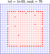
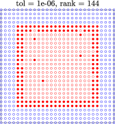
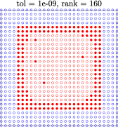
Figure 5. Illustration of ID with $4^{\rm th}$-order corrections described in Section 3.2. The red circles denote points in the box $\tau$ and the blue points denote the points in the proxy ring used. The solid red dots denote the points that correspond to skeleton indices, as chosen using CPQR as explained in Section 2.1. Each image corresponds to a specific compression tolerance, which is specified in the title, and also reported is the rank (i.e. the number of solid red circles) for that tolerance.

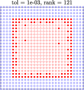
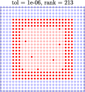
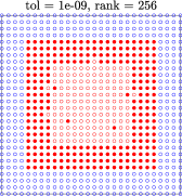
Figure 6. Analogue of Figure 5 for the $10^{\rm th}$-order quadrature corrections.

Remark 3.4.

A delicate question in building a rank-structured representation of a matrix is how to choose the local compression tolerance. Since errors do to some degree aggregate in the pass from smaller to larger blocks, it is advantageous to use a smaller (absolute) tolerance for boxes on the finest level, and then to gradually increase the tolerance parameter in the upwards pass. Deriving rigorous bounds on the error propagation is difficult, in particular when non-orthonormal basis matrices are used. Moreover, such bounds tend to be pessimistic since the worst-case alignment of the all error vectors is statistically extremely unlikely. In the numerical experiments reported in Section 6, we picked a local compression tolerance by multiplying a given global tolerance parameter $\varepsilon$ by (an estimate of) the Frobenius norm of the block to be compressed. This simple strategy automatically enforces more precise approximation of blocks at the finer levels, and has empirically proven to work well.

4. A direct solver based on discrete scattering operators

We are now ready to describe the inversion procedure for (9). In the following, we will assume that an HBS approximation to the matrix $\bm{\mathsf{G}}$ has been computed using the procedure described in Section 3.2 and therefore all necessary matrices, as described in Remark 3.1, have been computed. In Section 4.1, we give a formal description of our solver. This is followed by Section 4.2 which gives a brief outline of the solver’s complexity. Section 4.3 provides some discussion contextualizing our work in relation to some existing direct solvers.

4.1. Description of solver

For each node $\tau$, we introduce the notation

(16) $$\bm{\mathsf{q}}_{\tau}=\bm{\mathsf{q}}(\mathcal{I}_{\tau}),\quad\bm{\mathsf{w}}_{\tau}=\bm{\mathsf{G}}(\mathcal{I}_{\tau},\mathcal{I}_{\tau}^{c})\bm{\mathsf{q}}(\mathcal{I}_{\tau}^{c}),\quad\bm{\mathsf{f}}_{\tau}=\bm{\mathsf{f}}(\mathcal{I}_{\tau}).$$

The vector $\bm{\mathsf{q}}_{\tau}$ represents the restriction of $\bm{\mathsf{q}}$ to the points in $\tau$ and $\bm{\mathsf{w}}_{\tau}$ represents the incoming field on the points in $\tau$ generated from all of the points outside of $\tau$.

The key observation that enables our direct solver is that to represent the interactions between nodes, it suffices to work with compressed versions of these vectors. To this end, we define an outgoing expansion $\widetilde{\bm{\mathsf{q}}}_{\tau}$ and an incoming expansion $\widetilde{\bm{\mathsf{w}}}_{\tau}$ through the relations

(17) $$\widetilde{\bm{\mathsf{q}}}_{\tau}=\widehat{\bm{\mathsf{V}}}_{\tau}^{*}\bm{\mathsf{q}}_{\tau},\quad\bm{\mathsf{w}}_{\tau}=\widehat{\bm{\mathsf{U}}}_{\tau}\widetilde{\bm{\mathsf{w}}}_{\tau},$$

respectively, where $\widehat{\bm{\mathsf{U}}}_{\tau}$ and $\widehat{\bm{\mathsf{V}}}_{\tau}$ are the extended basis matrices defined in Section 3.1. The expansions $\widetilde{\bm{\mathsf{q}}}_{\tau}$ and $\widetilde{\bm{\mathsf{w}}}_{\tau}$ serve as proxies for $\bm{\mathsf{q}}_{\tau}$ and $\bm{\mathsf{w}}_{\tau}$, and are analogous to the multipole and local expansions in the fast multipole method [14]. The key to relating the two expansions is the following lemma, which states that the incoming expansion of a non-root node can be split into a sibling-sibling interaction plus a contribution from the incoming field of the parent:

Lemma 4.1.

Let $\tau$ be a parent node with children $\alpha$ and $\beta$. Then, with $\bm{\mathsf{G}}_{\alpha,\beta}$ and $\bm{\mathsf{G}}_{\beta,\alpha}$ defined by (15), we have

(18) $$\begin{bmatrix}\widetilde{\bm{\mathsf{w}}}_{\alpha}\\ \widetilde{\bm{\mathsf{w}}}_{\beta}\end{bmatrix}=\begin{bmatrix}\bm{\mathsf{0}}&\bm{\mathsf{G}}_{\alpha,\beta}\\ \bm{\mathsf{G}}_{\beta,\alpha}&\bm{\mathsf{0}}\end{bmatrix}\begin{bmatrix}\widetilde{\bm{\mathsf{q}}}_{\alpha}\\ \widetilde{\bm{\mathsf{q}}}_{\beta}\end{bmatrix}+\bm{\mathsf{U}}_{\tau}\widetilde{\bm{\mathsf{w}}}_{\tau},$$

whenever $\widehat{\bm{\mathsf{U}}}_{\alpha}$ and $\widehat{\bm{\mathsf{U}}}_{\beta}$ have full column rank.

Proof.

By definition of the extended basis matrices, the full incoming field on $\alpha$ and $\beta$ can be expressed by

$$\begin{bmatrix}\bm{\mathsf{w}}_{\alpha}\\ \bm{\mathsf{w}}_{\beta}\end{bmatrix} =\begin{bmatrix}\bm{\mathsf{0}}&\bm{\mathsf{G}}(\mathcal{I}_{\alpha},\mathcal{I}_{\beta})\\ \bm{\mathsf{G}}(\mathcal{I}_{\beta},\mathcal{I}_{\alpha})&\bm{\mathsf{0}}\end{bmatrix}\begin{bmatrix}\bm{\mathsf{q}}_{\alpha}\\ \bm{\mathsf{q}}_{\beta}\end{bmatrix}+\widehat{\bm{\mathsf{U}}}_{\tau}\bm{\mathsf{w}}_{\tau}$$

$$=\begin{bmatrix}\widehat{\bm{\mathsf{U}}}_{\alpha}&\bm{\mathsf{0}}\\ \bm{\mathsf{0}}&\widehat{\bm{\mathsf{U}}}_{\beta}\end{bmatrix}\begin{bmatrix}\bm{\mathsf{0}}&\bm{\mathsf{G}}_{\alpha,\beta}\\ \bm{\mathsf{G}}_{\beta,\alpha}&\bm{\mathsf{0}}\end{bmatrix}\begin{bmatrix}\widehat{\bm{\mathsf{V}}}_{\alpha}^{*}&\bm{\mathsf{0}}\\ \bm{\mathsf{0}}&\widehat{\bm{\mathsf{V}}}_{\beta}^{*}\end{bmatrix}\begin{bmatrix}\bm{\mathsf{q}}_{\alpha}\\ \bm{\mathsf{q}}_{\beta}\end{bmatrix}+\begin{bmatrix}\widehat{\bm{\mathsf{U}}}_{\alpha}&\bm{\mathsf{0}}\\ \bm{\mathsf{0}}&\widehat{\bm{\mathsf{U}}}_{\beta}\end{bmatrix}\bm{\mathsf{U}}_{\tau}\widetilde{\bm{\mathsf{w}}}_{\tau}$$

$$=\begin{bmatrix}\widehat{\bm{\mathsf{U}}}_{\alpha}&\bm{\mathsf{0}}\\ \bm{\mathsf{0}}&\widehat{\bm{\mathsf{U}}}_{\beta}\end{bmatrix}\left(\begin{bmatrix}\bm{\mathsf{0}}&\bm{\mathsf{G}}_{\alpha,\beta}\\ \bm{\mathsf{G}}_{\beta,\alpha}&\bm{\mathsf{0}}\end{bmatrix}\begin{bmatrix}\widetilde{\bm{\mathsf{q}}}_{\alpha}\\ \widetilde{\bm{\mathsf{q}}}_{\beta}\end{bmatrix}+\bm{\mathsf{U}}_{\tau}\widetilde{\bm{\mathsf{w}}}_{\tau}\right).$$

The result then follows from the fact that $\widehat{\bm{\mathsf{U}}}_{\alpha}$ and $\widehat{\bm{\mathsf{U}}}_{\beta}$ have full column rank and by (17)

$$\begin{bmatrix}\widetilde{\bm{\mathsf{w}}}_{\alpha}\\ \widetilde{\bm{\mathsf{w}}}_{\beta}\end{bmatrix}=\begin{bmatrix}\widehat{\bm{\mathsf{U}}}_{\alpha}^{\dagger}&\bm{\mathsf{0}}\\ \bm{\mathsf{0}}&\widehat{\bm{\mathsf{U}}}_{\beta}^{\dagger}\end{bmatrix}\begin{bmatrix}\bm{\mathsf{w}}_{\alpha}\\ \bm{\mathsf{w}}_{\beta}\end{bmatrix}.$$

∎

We are now in position to derive the solver, which follows the pattern of the solver in [20, Ch. 18], but with some accelerations that are enabled by the particular nature of the equilibrium equation (9).

The first stage consist of a sweep upwards through the hierarchical tree, going from smaller to larger boxes. To start, let $\tau$ denote a leaf box. Recalling the definition of local potentials in (16), and restricting the equilibrium equation (9) to $\tau$, we obtain the local equilibrium equation

(19) $$(\bm{\mathsf{I}}+\bm{\mathsf{B}}_{\tau}\bm{\mathsf{G}}_{\tau})\bm{\mathsf{q}}_{\tau}+\bm{\mathsf{B}}_{\tau}\bm{\mathsf{w}}_{\tau}=\bm{\mathsf{f}}_{\tau},$$

where $\bm{\mathsf{B}}_{\tau}=\bm{\mathsf{B}}(\mathcal{I}_{\tau},\mathcal{I}_{\tau})$ and $\bm{\mathsf{G}}_{\tau}=\bm{\mathsf{G}}(\mathcal{I}_{\tau},\mathcal{I}_{\tau})$. Setting

(20) $$\bm{\mathsf{X}}_{\tau}=(\bm{\mathsf{I}}+\bm{\mathsf{B}}_{\tau}\bm{\mathsf{G}}_{\tau})^{-1}$$

and then multiplying both sides of (19) by $\bm{\mathsf{V}}_{\tau}^{*}\bm{\mathsf{X}}_{\tau}$ produces

(21) $$\bm{\mathsf{V}}_{\tau}^{*}\bm{\mathsf{q}}_{\tau}+\bm{\mathsf{V}}_{\tau}^{*}\bm{\mathsf{X}}_{\tau}\bm{\mathsf{B}}_{\tau}\bm{\mathsf{w}}_{\tau}=\bm{\mathsf{V}}_{\tau}^{*}\bm{\mathsf{X}}_{\tau}\bm{\mathsf{f}}_{\tau}.$$

Using the fact that by definition $\widehat{\bm{\mathsf{V}}}_{\tau}=\bm{\mathsf{V}}_{\tau}$ for leaves, (21) can be rewritten using the notation in (17) as

(22) $$\widetilde{\bm{\mathsf{q}}}_{\tau}+\bm{\mathsf{S}}_{\tau}\widetilde{\bm{\mathsf{w}}}_{\tau}=\widetilde{\bm{\mathsf{r}}}_{\tau},$$

where

(23) $$\bm{\mathsf{S}}_{\tau}=\bm{\mathsf{V}}_{\tau}^{*}\bm{\mathsf{X}}_{\tau}\bm{\mathsf{B}}_{\tau}\bm{\mathsf{U}}_{\tau}$$

and

(24) $$\widetilde{\bm{\mathsf{r}}}_{\tau}=\bm{\mathsf{V}}_{\tau}^{*}\bm{\mathsf{X}}_{\tau}\bm{\mathsf{f}}_{\tau}.$$

The matrix $\bm{\mathsf{S}}_{\tau}$ can be viewed as a discrete analogue of a scattering matrix, which is a mathematical operator that encodes the relationship between the incoming field and the effective charge on a box in the absence of a source [5].

We next move one level up the tree and consider a parent node $\tau$ with leaf children $\alpha$ and $\beta$. Combining Lemma 4.1 and the fact that both $\alpha$ and $\beta$ satisfy (22), we have the equilibrium equation

(25) $$\begin{bmatrix}\widetilde{\bm{\mathsf{q}}}_{\alpha}\\ \widetilde{\bm{\mathsf{q}}}_{\beta}\end{bmatrix}+\begin{bmatrix}\bm{\mathsf{S}}_{\alpha}&\bm{\mathsf{0}}\\ \bm{\mathsf{0}}&\bm{\mathsf{S}}_{\beta}\end{bmatrix}\left(\begin{bmatrix}\bm{\mathsf{0}}&\bm{\mathsf{G}}_{\alpha,\beta}\\ \bm{\mathsf{G}}_{\beta,\alpha}&\bm{\mathsf{0}}\end{bmatrix}\begin{bmatrix}\widetilde{\bm{\mathsf{q}}}_{\alpha}\\ \widetilde{\bm{\mathsf{q}}}_{\beta}\end{bmatrix}+\bm{\mathsf{U}}_{\tau}\widetilde{\bm{\mathsf{w}}}_{\tau}\right)=\begin{bmatrix}\widetilde{\bm{\mathsf{r}}}_{\alpha}\\ \widetilde{\bm{\mathsf{r}}}_{\beta}\end{bmatrix}.$$

Setting

(26) $$\bm{\mathsf{X}}_{\tau}=\begin{bmatrix}\bm{\mathsf{I}}&\bm{\mathsf{S}}_{\alpha}\bm{\mathsf{G}}_{\alpha,\beta}\\ \bm{\mathsf{S}}_{\beta}\bm{\mathsf{G}}_{\beta,\alpha}&\bm{\mathsf{I}}\end{bmatrix}^{-1}$$

and then multiplying both sides of (25) by $\bm{\mathsf{V}}_{\tau}^{*}\bm{\mathsf{X}}_{\tau}$ produces

$$\bm{\mathsf{V}}_{\tau}^{*}\begin{bmatrix}\widetilde{\bm{\mathsf{q}}}_{\alpha}\\ \widetilde{\bm{\mathsf{q}}}_{\beta}\end{bmatrix}+\bm{\mathsf{V}}_{\tau}^{*}\bm{\mathsf{X}}_{\tau}\begin{bmatrix}\bm{\mathsf{S}}_{\alpha}&\bm{\mathsf{0}}\\ \bm{\mathsf{0}}&\bm{\mathsf{S}}_{\beta}\end{bmatrix}\bm{\mathsf{U}}_{\tau}\widetilde{\bm{\mathsf{w}}}_{\tau}=\bm{\mathsf{V}}_{\tau}^{*}\bm{\mathsf{X}}_{\tau}\begin{bmatrix}\widetilde{\bm{\mathsf{r}}}_{\alpha}\\ \widetilde{\bm{\mathsf{r}}}_{\beta}\end{bmatrix}.$$

Using (17) and defining

(27) $$\bm{\mathsf{S}}_{\tau}=\bm{\mathsf{V}}_{\tau}^{*}\bm{\mathsf{X}}_{\tau}\begin{bmatrix}\bm{\mathsf{S}}_{\alpha}&\bm{\mathsf{0}}\\ \bm{\mathsf{0}}&\bm{\mathsf{S}}_{\beta}\end{bmatrix}\bm{\mathsf{U}}_{\tau},$$

and

(28) $$\quad\widetilde{\bm{\mathsf{r}}}_{\tau}=\bm{\mathsf{V}}_{\tau}^{*}\bm{\mathsf{X}}_{\tau}\begin{bmatrix}\widetilde{\bm{\mathsf{r}}}_{\alpha}\\ \widetilde{\bm{\mathsf{r}}}_{\beta}\end{bmatrix}$$

gives us exactly (22) again, where now (27) allows us to compute the discrete scattering matrix for $\tau$ using the scattering matrices for its children, $\alpha$ and $\beta$. This allows us to recursively traverse up the tree, obtaining a relation identical to (22) at each level until we get to the root.

Now, let $\tau$ be the root and let $\alpha$ and $\beta$ be its children. Since there is no incoming field on $\tau$, the only incoming field on $\alpha$ is due to charges in $\beta$ and vice versa. Therefore, the equation analogous to (25) simplifies in this case to

(29) $$\begin{bmatrix}\bm{\mathsf{I}}&\bm{\mathsf{S}}_{\alpha}\bm{\mathsf{G}}_{\alpha,\beta}\\ \bm{\mathsf{S}}_{\beta}\bm{\mathsf{G}}_{\beta,\alpha}&\bm{\mathsf{I}}\end{bmatrix}\begin{bmatrix}\widetilde{\bm{\mathsf{q}}}_{\alpha}\\ \widetilde{\bm{\mathsf{q}}}_{\beta}\end{bmatrix}=\begin{bmatrix}\widetilde{\bm{\mathsf{r}}}_{\alpha}\\ \widetilde{\bm{\mathsf{r}}}_{\beta}\end{bmatrix},$$

which can be inverted directly. Then, the incoming fields on $\alpha$ and $\beta$ can be computed by the matrix-vector product

$$\begin{bmatrix}\widetilde{\bm{\mathsf{w}}}_{\alpha}\\ \widetilde{\bm{\mathsf{w}}}_{\beta}\end{bmatrix}=\begin{bmatrix}\bm{\mathsf{0}}&\bm{\mathsf{G}}_{\alpha,\beta}\\ \bm{\mathsf{G}}_{\beta,\alpha}&\bm{\mathsf{0}}\end{bmatrix}\begin{bmatrix}\widetilde{\bm{\mathsf{q}}}_{\alpha}\\ \widetilde{\bm{\mathsf{q}}}_{\beta}\end{bmatrix}.$$

The incoming and outgoing expansions of the nodes on other levels can be computed using a downward sweep, as follows. Let $\tau$ be a node, such that its parent has been processed and so the incoming expansion $\widetilde{\bm{\mathsf{w}}}_{\tau}$ has been computed. If $\alpha$ and $\beta$ are children of $\tau$, then using (25) and (26) we can obtain the equation for the outgoing expansions on $\alpha$ and $\beta$

$$\begin{bmatrix}\widetilde{\bm{\mathsf{q}}}_{\alpha}\\ \widetilde{\bm{\mathsf{q}}}_{\beta}\end{bmatrix}=\bm{\mathsf{X}}_{\tau}\left(\begin{bmatrix}\widetilde{\bm{\mathsf{r}}}_{\alpha}\\ \widetilde{\bm{\mathsf{r}}}_{\beta}\end{bmatrix}-\begin{bmatrix}\bm{\mathsf{S}}_{\alpha}&\bm{\mathsf{0}}\\ \bm{\mathsf{0}}&\bm{\mathsf{S}}_{\beta}\end{bmatrix}\bm{\mathsf{U}}_{\tau}\widetilde{\bm{\mathsf{w}}}_{\tau}\right).$$

The incoming expansions $\widetilde{\bm{\mathsf{w}}}_{\alpha}$ and $\widetilde{\bm{\mathsf{w}}}_{\beta}$ can then be computed using (18). We can proceed to compute the incoming and outgoing expansions for the children of $\alpha$ and $\beta$ and so on, all the way down the tree.

After the incoming expansion for a leaf node $\tau$ is determined, (19) and (17) are used to determine the solution of the original system through the equation

$$\bm{\mathsf{q}}_{\tau}=\bm{\mathsf{X}}_{\tau}\left(\bm{\mathsf{f}}_{\tau}-\bm{\mathsf{B}}_{\tau}\bm{\mathsf{U}}_{\tau}\widetilde{\bm{\mathsf{w}}}_{\tau}\right).$$

It is customary to split the solution process into a build stage in which the matrices that define the solution operator are all constructed, and a solve stage in which the computed approximate solution operator is applied to a given incoming field. In our setting, the build stage consists of a single pass up the tree in which the local solution operator $\bm{\mathsf{X}}_{\tau}$ and the local scattering matrix $\bm{\mathsf{S}}_{\tau}$ is computed for each node $\tau$. This is illustrated in Algorithm 1, which computes the local solution operators and scattering matrices on all nodes, first for the leaves using (20) and (23), and then for all other nodes in an upward pass using (26) and (27). Then, given a right-hand side vector, the solve stage consists of a pass up the tree, where the $\widetilde{\bm{\mathsf{r}}}_{\tau}$ are computed using (24) and (28), and then a downward pass where the incoming expansions $\widetilde{\bm{\mathsf{w}}}_{\tau}$ are computed. This procedure is summarized in Algorithm 2. In an environment where an inverse needs to be applied to multiple different vectors, such as in preconditioning or when one is interested in evaluating the scattered field for multiple incident fields, the build stage which is the dominant cost needs to be executed just once.

Remark 4.1.

A dominant cost of the build stage is the evaluation of the matrices $\bm{\mathsf{X}}_{\tau}$, as defined by (26). This computation can be accelerated by exploiting the presence of the two identity matrices on the diagonal and the fact that the matrices $\bm{\mathsf{G}}_{\alpha,\beta}$ and $\bm{\mathsf{G}}_{\beta,\alpha}$ tend to be substantially rank deficient. A heuristic argument for this rank deficiency is that the matrices $\bm{\mathsf{G}}_{\alpha,\beta}$ and $\bm{\mathsf{G}}_{\beta,\alpha}$ encode the interactions between the skeleton indices of two adjacent boxes. While these points typically live on the entire perimeter of each box (see Figures 5 and 6), the interactions can be accurately represented using mostly points on the single shared side. Thus, we expect the ranks of the off-diagonal blocks to be a little over 25% of their sizes, which can be leveraged for more efficient inversion.

To this end, suppose we have low rank factorizations $\bm{\mathsf{G}}_{\alpha,\beta}=\bm{\mathsf{L}}_{\alpha,\beta}\bm{\mathsf{R}}_{\alpha,\beta}^{*}$ and $\bm{\mathsf{G}}_{\beta,\alpha}=\bm{\mathsf{L}}_{\beta,\alpha}\bm{\mathsf{R}}_{\beta,\alpha}^{*}$, which can be computed once per level during the HBS compression at a modest cost. We can apply the Woodbury formula to (26) to get the equivalent formula for the local solution operator of a non-leaf node

(30) $$\bm{\mathsf{X}}_{\tau}=\bm{\mathsf{I}}-\begin{bmatrix}\bm{\mathsf{S}}_{\alpha}\bm{\mathsf{L}}_{\alpha,\beta}&\bm{\mathsf{0}}\\ \bm{\mathsf{0}}&\bm{\mathsf{S}}_{\beta}\bm{\mathsf{L}}_{\beta,\alpha}\end{bmatrix}\begin{bmatrix}\bm{\mathsf{I}}&\bm{\mathsf{R}}_{\beta,\alpha}^{*}\bm{\mathsf{L}}_{\beta,\alpha}\\ \bm{\mathsf{R}}_{\alpha,\beta}^{*}\bm{\mathsf{L}}_{\alpha,\beta}&\bm{\mathsf{I}}\end{bmatrix}^{-1}\begin{bmatrix}\bm{\mathsf{0}}&\bm{\mathsf{R}}_{\alpha,\beta}^{*}\\ \bm{\mathsf{R}}_{\beta,\alpha}^{*}&\bm{\mathsf{0}}\end{bmatrix}.$$

Note that the matrix that needs to be inverted in (30) is substantially smaller than that in (26).

Algorithm 1 Build inverse as described in Section 4.1

Input: HBS compression of coefficient matrix specified by $(\bm{\mathsf{U}}_{\tau},\bm{\mathsf{V}}_{\tau})$ for all non-root nodes, $(\bm{\mathsf{B}}_{\tau},\bm{\mathsf{G}}_{\tau}$) for all leaves, and $(\bm{\mathsf{G}}_{\alpha,\beta},\bm{\mathsf{G}}_{\beta,\alpha})$ for all parents with children $\alpha$ and $\beta$
Output: Inverse of HBS matrix specified by $\bm{\mathsf{X}}_{\tau}$ for all nodes and $\bm{\mathsf{S}}_{\tau}$ for all non-root nodes

1:for all $\tau$ a leaf do

2:     $\bm{\mathsf{X}}_{\tau}=(\bm{\mathsf{I}}+\bm{\mathsf{B}}_{\tau}\bm{\mathsf{G}}_{\tau})^{-1}$

3:     $\bm{\mathsf{S}}_{\tau}=\bm{\mathsf{V}}_{\tau}^{*}\bm{\mathsf{X}}_{\tau}\bm{\mathsf{B}}_{\tau}\bm{\mathsf{U}}_{\tau}$

4:end for

5:for $\ell$ = $L-1$, $L-3$, …, 0 do

6:     for all $\tau$ on level $\ell$ do

7:         $[\alpha,\beta]\leftarrow$ children of $\tau$

8:         $\bm{\mathsf{X}}_{\tau}=\begin{bmatrix}\bm{\mathsf{I}}&\bm{\mathsf{S}}_{\alpha}\bm{\mathsf{G}}_{\alpha,\beta}\\ \bm{\mathsf{S}}_{\beta}\bm{\mathsf{G}}_{\beta,\alpha}&\bm{\mathsf{I}}\end{bmatrix}^{-1}$

9:         if $\ell\neq 0$ then

10:              $\bm{\mathsf{S}}_{\tau}=\bm{\mathsf{V}}_{\tau}^{*}\bm{\mathsf{X}}_{\tau}\begin{bmatrix}\bm{\mathsf{S}}_{\alpha}&\bm{\mathsf{0}}\\ \bm{\mathsf{0}}&\bm{\mathsf{S}}_{\beta}\end{bmatrix}\bm{\mathsf{U}}_{\tau}$

11:         end if

12:     end for

13:end for

Algorithm 2 Apply inverse to right-hand side $\bm{\mathsf{f}}$ as described in Section 4.1

Input: HBS matrix, its inverse as in Algorithm 1, and right-hand side $\bm{\mathsf{f}}$
Output: Solution vector $\bm{\mathsf{q}}$
 

1:// Upwards pass

2:for all $\tau$ a leaf do

3:     $\bm{\mathsf{r}}_{\tau}=\bm{\mathsf{X}}_{\tau}\bm{\mathsf{f}}_{\tau}$

4:     $\widetilde{\bm{\mathsf{r}}}_{\tau}=\bm{\mathsf{V}}_{\tau}^{*}\bm{\mathsf{r}}_{\tau}$

5:end for

6:for $\ell$ = $L-1$, $L-3$, …, 1 do

7:     for all $\tau$ on level $\ell$ do

8:         $[\alpha,\beta]\leftarrow$ children of $\tau$

9:         $\widetilde{\bm{\mathsf{r}}}_{\tau}=\bm{\mathsf{V}}_{\tau}^{*}\bm{\mathsf{X}}_{\tau}\begin{bmatrix}\widetilde{\bm{\mathsf{r}}}_{\alpha}\\ \widetilde{\bm{\mathsf{r}}}_{\beta}\end{bmatrix}$

10:     end for

11:end for

12:// Top-level solve

13:$\tau\leftarrow$ root

14:$[\alpha,\beta]\leftarrow$ children of $\tau$

15:$\begin{bmatrix}\widetilde{\bm{\mathsf{w}}}_{\alpha}\\ \widetilde{\bm{\mathsf{w}}}_{\beta}\end{bmatrix}=\begin{bmatrix}\bm{\mathsf{0}}&\bm{\mathsf{G}}_{\alpha,\beta}\\ \bm{\mathsf{G}}_{\beta,\alpha}&\bm{\mathsf{0}}\end{bmatrix}\bm{\mathsf{X}}_{\tau}\begin{bmatrix}\widetilde{\bm{\mathsf{r}}}_{\alpha}\\ \widetilde{\bm{\mathsf{r}}}_{\beta}\end{bmatrix}$

16:// Downwards pass

17:for $\ell=2,3,\ldots,L-1$ do

18:     for all $\tau$ on level $\ell$ do

19:         $[\alpha,\beta]\leftarrow$ children of $\tau$

20:         $\begin{bmatrix}\widetilde{\bm{\mathsf{q}}}_{\alpha}\\ \widetilde{\bm{\mathsf{q}}}_{\beta}\end{bmatrix}=\bm{\mathsf{X}}_{\tau}\left(\begin{bmatrix}\widetilde{\bm{\mathsf{r}}}_{\alpha}\\ \widetilde{\bm{\mathsf{r}}}_{\beta}\end{bmatrix}-\begin{bmatrix}\bm{\mathsf{S}}_{\alpha}&\bm{\mathsf{0}}\\ \bm{\mathsf{0}}&\bm{\mathsf{S}}_{\beta}\end{bmatrix}\bm{\mathsf{U}}_{\tau}\widetilde{\bm{\mathsf{w}}}_{\tau}\right)$

21:         $\begin{bmatrix}\widetilde{\bm{\mathsf{w}}}_{\alpha}\\ \widetilde{\bm{\mathsf{w}}}_{\beta}\end{bmatrix}=\begin{bmatrix}\bm{\mathsf{0}}&\bm{\mathsf{G}}_{\alpha,\beta}\\ \bm{\mathsf{G}}_{\beta,\alpha}&\bm{\mathsf{0}}\end{bmatrix}\begin{bmatrix}\widetilde{\bm{\mathsf{q}}}_{\alpha}\\ \widetilde{\bm{\mathsf{q}}}_{\beta}\end{bmatrix}+\bm{\mathsf{U}}_{\tau}\widetilde{\bm{\mathsf{w}}}_{\tau}$

22:     end for

23:end for

24:// Form solution vector

25:for all $\tau$ a leaf do

26:     $\bm{\mathsf{q}}_{\tau}=\bm{\mathsf{r}}_{\tau}-\bm{\mathsf{X}}_{\tau}\bm{\mathsf{B}}_{\tau}\bm{\mathsf{U}}_{\tau}\widetilde{\bm{\mathsf{w}}}_{\tau}$

27:end for

4.2. Complexity estimate

The computational complexity of our solver depends on the numerical ranks of the off-diagonal blocks in the HBS format. For a 2D volume kernel like (2), the interaction rank of a box grows like the square root of the number of points it contains when the wavenumber and compression tolerance are fixed [18, Sec. 4]. Since the HBS compression and inversion stages use cubic dense linear algebra, the cost of each is dominated by the cost of processing the root level where the rank of interaction grows as $\mathcal{O}(N^{1/2})$, and thus both stages require $\mathcal{O}(N^{3/2})$ operations. Applying the inverse to a vector requires an operation that grows quadratically with the rank of each box, so each level requires $\mathcal{O}(N)$ operations, for a total of $\mathcal{O}(N\log N)$ operations. As for memory, besides the HBS factors the only matrices that need be stored for the inverse are the local solution operators $\bm{\mathsf{X}}_{\tau}$, and so the cost of storage is still $\mathcal{O}(N)$. For a more detailed analysis of the costs of solvers for HBS matrices, we refer the reader to [18, Sec. 4], which applies in our setting as well.

Remark 4.2 (Complexity for a fixed PDE).

In the case where $\kappa$ is kept fixed as $N$ is increased, it should be possible to reduce the $\mathcal{O}(N^{3/2})$ cost of the inversion stage to $\mathcal{O}(N)$ using techniques such as HIF [19], nested trees [9], or strong recursive skeletonization [23]. This is the subject of ongoing work.

Remark 4.3 (Complexity for a fixed number of points per wavelength).

In the case where $\kappa$ is increased as $N$ grows to keep a fixed number of discretization points per wavelength (so that $\kappa\sim N^{1/2}$), the overall complexity of the solver is $\mathcal{O}(\kappa^{3})$. In this case, the acceleration techniques referenced in Remark 4.2 do not apply, and we are not aware of any direct solvers that scale better than $\mathcal{O}(\kappa^{3})$ in the general case.

4.3. Comparison with existing solvers

The connection between the procedure described in Section 4.1 and some existing work on HBS-based direct solvers can be elucidated through the use of the sparse matrix embeddings introduced in [18]. For the equation (9) and an HBS tree with only two levels, the corresponding matrix embedding is given by

(31) $$\begin{bmatrix}(\bm{\mathsf{I}}+\bm{\mathsf{B}}_{\alpha}\bm{\mathsf{G}}_{\alpha})&\bm{\mathsf{0}}&\bm{\mathsf{B}}_{\alpha}\bm{\mathsf{U}}_{\alpha}&\bm{\mathsf{0}}&\bm{\mathsf{0}}&\bm{\mathsf{0}}\\ \bm{\mathsf{0}}&(\bm{\mathsf{I}}+\bm{\mathsf{B}}_{\beta}\bm{\mathsf{G}}_{\beta})&\bm{\mathsf{0}}&\bm{\mathsf{B}}_{\beta}\bm{\mathsf{U}}_{\beta}&\bm{\mathsf{0}}&\bm{\mathsf{0}}\\ -\bm{\mathsf{V}}_{\alpha}^{*}&\bm{\mathsf{0}}&\bm{\mathsf{0}}&\bm{\mathsf{0}}&\bm{\mathsf{I}}&\bm{\mathsf{0}}\\ \bm{\mathsf{0}}&-\bm{\mathsf{V}}_{\beta}^{*}&\bm{\mathsf{0}}&\bm{\mathsf{0}}&\bm{\mathsf{0}}&\bm{\mathsf{I}}\\ \bm{\mathsf{0}}&\bm{\mathsf{0}}&-\bm{\mathsf{I}}&\bm{\mathsf{0}}&\bm{\mathsf{0}}&\bm{\mathsf{G}}_{\alpha,\beta}\\ \bm{\mathsf{0}}&\bm{\mathsf{0}}&\bm{\mathsf{0}}&-\bm{\mathsf{I}}&\bm{\mathsf{G}}_{\beta,\alpha}&\bm{\mathsf{0}}\end{bmatrix}\begin{bmatrix}\bm{\mathsf{q}}_{\alpha}\\ \bm{\mathsf{q}}_{\beta}\\ \widetilde{\bm{\mathsf{w}}}_{\alpha}\\ \widetilde{\bm{\mathsf{w}}}_{\beta}\\ \widetilde{\bm{\mathsf{q}}}_{\alpha}\\ \widetilde{\bm{\mathsf{q}}}_{\beta}\\ \end{bmatrix}=\begin{bmatrix}\bm{\mathsf{f}}_{\alpha}\\ \bm{\mathsf{f}}_{\beta}\\ \bm{\mathsf{0}}\\ \bm{\mathsf{0}}\\ \bm{\mathsf{0}}\\ \bm{\mathsf{0}}\\ \end{bmatrix}.$$

Upon eliminating $\bm{\mathsf{q}}_{\alpha}$ and $\bm{\mathsf{q}}_{\beta}$ in the equations for $\widetilde{\bm{\mathsf{w}}}_{\alpha}$ and $\widetilde{\bm{\mathsf{w}}}_{\beta}$, the system

(32) $$\begin{bmatrix}\bm{\mathsf{S}}_{\alpha}&\bm{\mathsf{0}}&\bm{\mathsf{I}}&\bm{\mathsf{0}}\\ \bm{\mathsf{0}}&\bm{\mathsf{S}}_{\beta}&\bm{\mathsf{0}}&\bm{\mathsf{I}}\\ -\bm{\mathsf{I}}&\bm{\mathsf{0}}&\bm{\mathsf{0}}&\bm{\mathsf{G}}_{\alpha,\beta}\\ \bm{\mathsf{0}}&-\bm{\mathsf{I}}&\bm{\mathsf{G}}_{\beta,\alpha}&\bm{\mathsf{0}}\end{bmatrix}\begin{bmatrix}\widetilde{\bm{\mathsf{w}}}_{\alpha}\\ \widetilde{\bm{\mathsf{w}}}_{\beta}\\ \widetilde{\bm{\mathsf{q}}}_{\alpha}\\ \widetilde{\bm{\mathsf{q}}}_{\beta}\\ \end{bmatrix}=\begin{bmatrix}\widetilde{\bm{\mathsf{r}}}_{\alpha}\\ \widetilde{\bm{\mathsf{r}}}_{\beta}\\ \bm{\mathsf{0}}\\ \bm{\mathsf{0}}\\ \end{bmatrix}$$

is obtained, where we continue to use the notation of Section 4.1. The classical Woodbury inversion formula for HBS matrices as discussed in [13] corresponds to using the (1, 1) and (2, 2) blocks in (32) to eliminate $\widetilde{\bm{\mathsf{w}}}_{\alpha}$ and $\widetilde{\bm{\mathsf{w}}}_{\beta}$ to obtain

(33) $$\begin{bmatrix}\bm{\mathsf{S}}_{\alpha}^{-1}&\bm{\mathsf{G}}_{\alpha,\beta}\\ \bm{\mathsf{G}}_{\beta,\alpha}&\bm{\mathsf{S}}_{\beta}^{-1}\end{bmatrix}\begin{bmatrix}\widetilde{\bm{\mathsf{q}}}_{\alpha}\\ \widetilde{\bm{\mathsf{q}}}_{\beta}\\ \end{bmatrix}=\begin{bmatrix}\bm{\mathsf{S}}_{\alpha}^{-1}\widetilde{\bm{\mathsf{r}}}_{\alpha}\\ \bm{\mathsf{S}}_{\beta}^{-1}\widetilde{\bm{\mathsf{r}}}_{\beta}\\ \end{bmatrix}.$$

This requires inverting both $\bm{\mathsf{S}}_{\alpha}$ and $\bm{\mathsf{S}}_{\beta}$, which in our application is often highly ill-conditioned due to $\bm{\mathsf{B}}$ in (9) containing small diagonal entries. Indeed, for the problems in Section 6, we frequently encounter scattering matrices with condition numbers far greater than the reciprocal of machine precision in double-precision arithmetic.

The scheme described in Section 4.1, on the other hand, uses the (3, 1) and (4, 2) blocks in (32) as pivots. This leads to the mathematically equivalent system

(34) $$\begin{bmatrix}\bm{\mathsf{I}}&\bm{\mathsf{S}}_{\alpha}\bm{\mathsf{G}}_{\alpha,\beta}\\ \bm{\mathsf{S}}_{\beta}\bm{\mathsf{G}}_{\beta,\alpha}&\bm{\mathsf{I}}\end{bmatrix}\begin{bmatrix}\widetilde{\bm{\mathsf{q}}}_{\alpha}\\ \widetilde{\bm{\mathsf{q}}}_{\beta}\\ \end{bmatrix}=\begin{bmatrix}\widetilde{\bm{\mathsf{r}}}_{\alpha}\\ \widetilde{\bm{\mathsf{r}}}_{\beta}\\ \end{bmatrix}.$$

Solving (34) is often a more benign operation, since the coefficient matrix is a perturbation to the identity. In particular, in regions where the scattering potential is small in magnitude, the “perturbation terms” $\bm{\mathsf{S}}_{\alpha}\bm{\mathsf{G}}_{\alpha\beta}$ and $\bm{\mathsf{S}}_{\beta}\bm{\mathsf{G}}_{\beta\alpha}$ will be of small magnitude too, which ensures that (34) is well-conditioned. In other words, the formulation (34) avoids the “spurious” ill-conditioning issues in (33). In addition, the resulting solvers require fewer arithmetic operations.

The approach suggested in [18] is to apply a sparse direct solver package, such as UMFPACK, to the entire system (31). Such packages have highly optimized algorithms for selecting pivots to minimize fill-in, while avoiding the inversion of ill-conditioned matrices. In our experiments, we find this strategy is as robust as our solver, but we empirically find the approach of [18] to be slower and more memory-intensive than the technique described here.

5. Using the solver as a preconditioner

The computational cost of the direct solver that we have described depends strongly on the requested accuracy, for two reasons. First, as the compression tolerance goes to zero, all interaction ranks increase, and since the solver relies on dense linear algebra, its overall run time scales cubically with the numerical ranks. Second, in order to attain high accuracy, the high-order accurate version of Duan-Rokhlin quadrature must be used, which as discussed in Section 3.2 increases the ranks even further.

When high accuracy is desired, the best approach is often to run the direct solver that we have described at low accuracy, and then use the computed rough inverse as a preconditioner. This turns out to be remarkably effective due to the fact that the $4^{\rm th}$-order accurate Duan-Rokhlin quadrature involves only the diagonal entries of the matrix, which means that they do not impact the compression of the off-diagonal blocks at all.

To describe the idea in more detail, suppose that we seek to solve a high-order discretization such as, cf. (9),

$$(\bm{\mathsf{I}}+\bm{\mathsf{B}}\bm{\mathsf{G}}+\bm{\mathsf{B}}\bm{\mathsf{T}})\bm{\mathsf{q}}=\bm{\mathsf{f}},$$

where $\bm{\mathsf{G}}$ is defined by (10) (representing the $O(h^{4})$ order accurate discretization of the integral operator), and where $\bm{\mathsf{T}}$ is the necessary “correction” matrix for a $10^{\rm th}$-order discretization. In other words, $\bm{\mathsf{T}}$ contains the $10^{\rm th}$-order corrections minus the $4^{\rm th}$-order corrections. The idea is now to build a rough approximate inverse $\bm{\mathsf{M}}$ to the more compressible $4^{\rm th}$-order discretization of the operator, so that

$$\bm{\mathsf{M}}\approx\bigl{(}\bm{\mathsf{I}}+\bm{\mathsf{B}}\bm{\mathsf{G}}\bigr{)}^{-1}.$$

We then apply GMRES to the preconditioned system

$$\bm{\mathsf{M}}(\bm{\mathsf{I}}+\bm{\mathsf{B}}\bm{\mathsf{G}}+\bm{\mathsf{B}}\bm{\mathsf{T}})\bm{\mathsf{q}}=\bm{\mathsf{M}}\bm{\mathsf{f}},$$

exploiting that the original operator $\bm{\mathsf{I}}+\bm{\mathsf{B}}\bm{\mathsf{G}}+\bm{\mathsf{B}}\bm{\mathsf{T}}$ can be applied rapidly to vectors since $\bm{\mathsf{B}}$ is sparse, and $\bm{\mathsf{G}}+\bm{\mathsf{T}}$ is a convolution operator that be applied through the FFT (see [10] for details).

The left image in Figure 7 displays the spectrum in the complex plane of a discretization of the left-hand side of (3) using 1600 degrees of freedom with $10^{\rm th}$-order quadrature corrections, where $\kappa=8\pi$, so that each side of $\Omega$ is 4 vacuum wavelengths across, and the scattering potential was chosen to be the lens described in Section 6.3. While most of the eigenvalues cluster near 1 reflecting the fact that (3) is a second-kind Fredholm integral equation, there are many eigenvalues that are located far from 1. As a result, an iterative method, such as GMRES, will converge quite slowly. For example, for a right-hand side corresponding to a plane wave, GMRES takes 62 iterations to reach a tolerance of $10^{-5}$ and 80 iterations to reach a tolerance of $10^{-10}$.

The image on the right of Figure 7 shows the spectrum after preconditioning with the direct solver with compression tolerance $10^{-2}$ and the $4^{\rm th}$-order quadrature corrections. Now, all of the eigenvalues are clustered closely to 1, which means that GMRES will converge in just a few iterations, even if high accuracy is required. (In fact, all eigenvalues are within distance 0.06 from 1!) For the same plane wave as in the previous paragraph, GMRES now only takes 3 iterations to converge to a tolerance of $10^{-5}$ and 6 iterations to converge to a tolerance of $10^{-10}$. Furthermore, for this example, building the preconditioner takes only a fraction of a second on a laptop computer and each preconditioned iteration is only twice as slow as an iteration without any preconditioning.

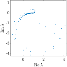
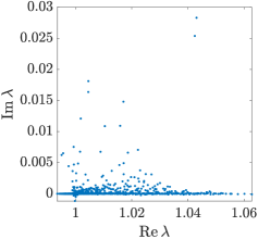
Figure 7. Spectra of unpreconditioned (left) and preconditioned (right) discretization of Lippmann-Schwinger equation with $\kappa=8\pi$, 1600 degrees of freedom, $10^{\rm th}$-order quadrature corrections, and the lens potential as described in Section 6.3. Observe the scale in the figure to the right; all eigenvalues are very close to one.

6. Numerical experiments

We present three sets of numerical experiments: In Section 6.1, we study the scaling of our solver with respect to mesh refinement for a scattering potential given by a Gaussian bump. We empirically verify the theoretical estimates in Section 4.2. This is followed by Section 6.2, where we examine the case of scattering against a cavity. We end on Section 6.3 which demonstrates how our solver can be used as a preconditioner as motivated in Section 5. Here we consider scattering against a cavity in the regime where the wavenumber is increased with the number of points per wavelength held constant, and also four challenging problems introduced in [12]. All timings are reported on a workstation with 2 Intel Xeon Gold 6254 (18 cores at 3.1GHz base frequency) processors with 768 GB of RAM.

6.1. The direct solver applied to a Gaussian scattering potential

We first study the case where the scattering potential is given by $b(\bm{x})=1.5\exp(-160\|\bm{x}\|^{2})$ as shown in the left plot in Figure 8. The wavenumber is set to $\kappa=25$, so that $\Omega$ is approximately 4 wavelengths wide, and the incident field is taken to be the plane wave $u^{\rm inc}(\bm{x})=\exp(i\kappa x_{1})$. We run the direct solver with compression tolerances $10^{-3}$, $10^{-6}$, $10^{-9}$ and $10^{-12}$ with the $10^{\rm th}$-order quadrature corrections. For each choice of compression tolerance, we keep the number of degrees of freedom in a leaf node of the HBS tree constant at 100, increase the number of levels in the tree, and note the following quantities:

$N$	The total number of degrees of freedom.
$h$	The mesh width. Note that $h=1/\sqrt{N}$.
$T_{\rm skel}$	Time in seconds to compute the HBS approximation.
$T_{\rm build}$	Time in seconds to invert the HBS approximation.
$T_{\rm apply}$	Time in seconds to apply the inverse a single time.
mem	Total memory in GB used to store both the HBS approximation and its inverse.
res	The relative residual error in the computed solution.

The results are summarized in Tables 2–5. The total field is shown in the right plot of Figure 8.

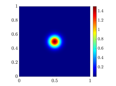
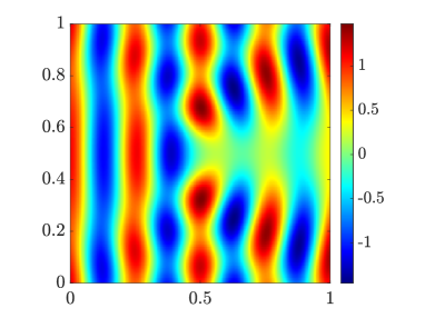
Figure 8. Left: Scattering potential for Gaussian bump in Section 6.1. Right: Total field for Section 6.1.

$N$	$h$	$T_{\rm skel}$	$T_{\rm build}$	$T_{\rm apply}$	mem	res
6400	0.0125	1.35	0.40	0.05	0.12	7.74e-05
25600	0.00625	5.51	1.77	0.12	0.60	5.71e-05
102400	0.003125	28.78	9.07	0.48	2.94	9.75e-05
409600	0.0015625	128.50	39.35	2.00	12.14	1.56e-04
1638400	0.00078125	680.04	165.15	10.53	48.59	5.77e-04

Table 2. Data for Section 6.1 with compression tolerance $10^{-3}$.

$N$	$h$	$T_{\rm skel}$	$T_{\rm build}$	$T_{\rm apply}$	mem	res
6400	0.0125	2.30	0.86	0.07	0.27	9.54e-09
25600	0.00625	11.57	4.43	0.19	1.42	7.13e-08
102400	0.003125	56.32	22.93	0.76	6.86	4.15e-08
409600	0.0015625	328.92	114.94	6.58	31.33	4.39e-08
1638400	0.00078125	2201.34	590.61	33.50	145.71	3.14e-07

Table 3. Data for Section 6.1 with compression tolerance $10^{-6}$.

$N$	$h$	$T_{\rm skel}$	$T_{\rm build}$	$T_{\rm apply}$	mem	res
6400	0.0125	2.82	1.22	0.07	0.36	1.57e-12
25600	0.00625	16.48	6.91	0.24	1.98	3.37e-12
102400	0.003125	80.08	37.49	1.04	10.01	1.45e-11
409600	0.0015625	475.07	200.59	6.82	48.22	3.48e-09
1638400	0.00078125	3139.07	1023.81	67.17	225.26	2.99e-09

Table 4. Data for Section 6.1 with compression tolerance $10^{-9}$.

$N$	$h$	$T_{\rm skel}$	$T_{\rm build}$	$T_{\rm apply}$	mem	res
6400	0.0125	2.99	1.41	0.07	0.38	1.87e-15
25600	0.00625	15.90	7.80	0.22	2.11	3.80e-15
102400	0.003125	83.22	42.56	1.00	10.82	6.94e-15
409600	0.0015625	529.54	237.64	5.98	52.79	1.71e-14
1638400	0.00078125	3474.55	1304.09	47.13	250.27	5.07e-14

Table 5. Data for Section 6.1 with compression tolerance $10^{-12}$.

Figure 9 provides plots that compare the observed timings with the estimates of the asymptotic complexity in Section 4.2. The empirical results indicate slightly better scaling than the predicted $O(N^{3/2})$ complexity, but this effect is merely due to the fact that the true asymptotic has not yet had a chance to establish itself at these problem sizes. Looking at the prefactors in the scalings, we see that compression is significantly slower than inversion. As the compression tolerance $\epsilon$ goes to zero, the prefactors grow at an observed rate of between $O(\log(1/\epsilon))$ and $O((\log(1/\epsilon))^{2})$.

Remark 6.1.

It is interesting to note that in Tables 2–5 the residual errors tend to grow with the number of degrees of freedom. This is due to the accumulation of errors in compression as the number of levels in the tree increase, cf. Remark 3.4. Nonetheless, the residuals here are all close to the HBS compression tolerance.

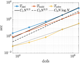
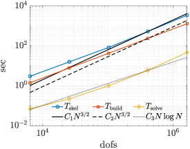
Figure 9. Scaling of HBS compression, inversion, and inverse application for experiment in Section 6.1 with compression tolerances $10^{-3}$ (top left), $10^{-6}$ (top right), $10^{-9}$ (bottom left), and $10^{-12}$ (bottom right).

6.2. The direct solver applied to a cavity problem

Solutions to the problem considered in Section 6.1 do not involve any backscattering; a fact that makes the problem highly amenable to iterative methods. Indeed, it was found in [10] that for such a potential even an iterative method without preconditioning converges in just a few iterations, although a direct solver might still be better-suited when one is interested in scattering for multiple incident fields.

We now consider a cavity potential given in polar coordinates by

$$b(r,\theta)=(1-\sin(0.5\theta)^{500})\exp(-2000(0.1-r^{2})^{2})$$

(see the left image in Figure 10). Without preconditioning, the number of GMRES iterations required to solve even relatively low frequency scattering to a couple of digits is unfeasibly high, due to the near-resonant behavior of the problem. We repeat the experiments of the previous section for this scattering potential when $\kappa=50.27$, so that $\Omega$ is about 8 wavelengths across. The results are given in Tables 6–9 and Figure 11. The total field is plotted in the right of Figure 10.

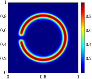
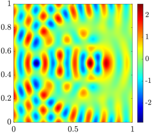
Figure 10. Left: Scattering potential for Section 6.2. Right: Total field for $\kappa=50.27$.

$N$	$h$	$T_{\rm skel}$	$T_{\rm build}$	$T_{\rm apply}$	mem	res
6400	0.0125	2.21	0.46	0.05	0.15	6.42e-05
25600	0.00625	5.36	2.16	0.14	0.67	2.82e-04
102400	0.003125	30.70	9.63	0.77	3.08	3.68e-04
409600	0.0015625	167.84	46.80	3.09	14.52	6.86e-04
1638400	0.00078125	940.77	222.96	13.16	65.10	1.14e-03

Table 6. Data for Section 6.2 with compression tolerance $10^{-3}$.

$N$	$h$	$T_{\rm skel}$	$T_{\rm build}$	$T_{\rm apply}$	mem	res
6400	0.0125	2.42	0.94	0.07	0.30	9.52e-08
25600	0.00625	12.59	4.97	0.42	1.57	5.89e-08
102400	0.003125	60.27	25.71	1.12	7.64	5.54e-07
409600	0.0015625	360.95	130.26	6.52	35.64	5.75e-07
1638400	0.00078125	2280.63	645.20	25.84	158.14	1.09e-06

Table 7. Data for Section 6.2 with compression tolerance $10^{-6}$.

$N$	$h$	$T_{\rm skel}$	$T_{\rm build}$	$T_{\rm apply}$	mem	res
6400	0.0125	2.61	1.11	0.07	0.36	4.23e-11
25600	0.00625	15.81	6.54	0.21	2.01	7.40e-11
102400	0.003125	79.86	36.36	1.06	10.38	2.67e-10
409600	0.0015625	491.72	206.02	9.55	50.42	4.59e-10
1638400	0.00078125	3289.37	1109.28	25.72	234.48	1.02e-08

Table 8. Data for Section 6.2 with compression tolerance $10^{-9}$.

$N$	$h$	$T_{\rm skel}$	$T_{\rm build}$	$T_{\rm apply}$	mem	res
6400	0.0125	2.72	1.23	0.06	0.39	3.28e-14
25600	0.00625	16.34	7.20	0.21	2.15	1.03e-13
102400	0.003125	82.90	40.68	1.16	10.95	6.29e-13
409600	0.0015625	515.89	227.17	5.08	53.34	3.36e-12
1638400	0.00078125	3495.09	1304.42	48.21	252.23	1.02e-11

Table 9. Data for Section 6.2 with compression tolerance $10^{-12}$.

Besides a marginal increase in cost due to the slightly higher wavenumber, the results are practically identical to those for the Gaussian bump. This illustrates the fact that the direct solver, unlike iterative solvers, is agnostic to features of the scattering potential.

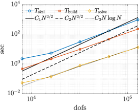
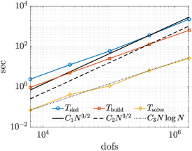
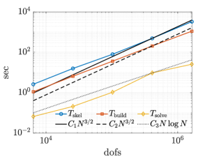
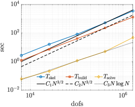
Figure 11. Scaling of HBS compression, inversion, and inverse application for direct solver experiment in Section 6.2 with compression tolerances $10^{-3}$ (top left), $10^{-6}$ (top right), $10^{-9}$ (bottom left), and $10^{-12}$ (bottom right).

6.3. Using an approximate inverse as a preconditioner

We will next demonstrate the effectiveness of using the direct solver as a preconditioner. We recall from Section 5 that the idea is to use a low-order quadrature with a small correction stencil in order to improve compressibility of the off-diagonal blocks of the coefficient matrix, and a lower compression tolerance to obtain a leaner representation. The resulting inverse is too rough to use as a direct solver for the highly ill-conditioned problems under consideration, but is an excellent preconditioner.

For an initial experiment, we stick with the cavity problem described in Section 6.2. We use the a compression tolerance of $10^{-4}$ and a $4^{\rm th}$-order quadrature corrections to build the preconditioner for the GMRES iteration. The matrix-vector product is executed using the coefficient matrix with $10^{\rm th}$-order corrections applied using the FFT as discussed in Section 2.2. We apply this approach to the cavity scattering potential where the number of points per wavelength is kept fixed at 10 and the wavenumber is increased, with GMRES set to terminate when the norm of the relative residual is below $10^{-10}$. In addition to the relevant previously defined quantities, we also examine:

$T_{\rm gmres}$	Total time spent by GMRES.
iter	The number of GMRES iterations required to reach a relative residual with norm below $10^{-10}$.

Table 10 reports these results for computational domains ranging from approximately 8 to 512 wavelengths across. The total field when $\kappa=201.06$ and $\kappa=804.25$ are displayed in the left and right plots of Figure 12, respectively.

$N$	$\kappa$	$T_{\rm skel}$	$T_{\rm build}$	$T_{\rm gmres}$	mem	iter	res
6400	50.27	0.23	0.24	0.20	0.04	4	6.97e-11
25600	100.53	0.65	0.99	0.62	0.21	5	6.16e-12
102400	201.06	2.26	4.36	2.49	1.01	6	1.04e-12
409600	402.12	14.91	20.06	9.78	4.67	6	3.23e-11
1638400	804.25	99.01	91.37	56.13	21.16	9	8.12e-12
6553600	1608.50	430.60	398.88	330.91	94.63	13	3.93e-11
26214400	3216.99	3102.09	2024.16	2698.53	418.37	22	3.30e-11

Table 10. Data for preconditioned iterative solver for the cavity problem in Section 6.3.

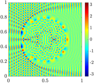
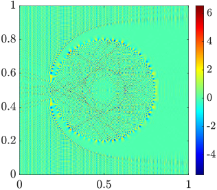
Figure 12. Total field for $\kappa=201.06$ (left) and $\kappa=804.25$ (right) for cavity potential in Figure 10.

Without preconditioning, the problems in the larger domains in Table 10 would require thousands of GMRES iterations to achieve convergence to a tolerance that yields accuracy for these intrinsically ill-conditioned problems. To investigate whether the excellent performance we observed for the cavity problem was a fluke or is the universal behavior of the preconditioner, we next consider four challenging test problems that were introduced in [12]:

Lens:	A vertically-graded lens given by $b(\bm{x})=4(x_{2}-0.1)[1-\operatorname{erf}(25(\|\bm{x}\|-0.3))]$ with $\kappa=300$ (Figure 13, top left). The incident field is given by a plane wave $u^{\rm inc}(\bm{x})=\exp(i\kappa(x_{1}-0.5))$. The computational domain is about 47.7 vacuum wavelengths across.
Random bumps:	The sum of 200 Gaussian bumps randomly placed in $\Omega$ and rolled off to zero in a smooth fashion with $\kappa=160$ (Figure 13, top right). The incident field is given by a plane wave $u^{\rm inc}(\bm{x})=\exp(i\kappa(x_{1}-0.5))$. The computational domain is about 25.5 vacuum wavelengths across.
Photonic crystal:	A 20 by 20 square grid of Gaussian bumps with a channel removed with $\kappa=77.1$ (the first complete band gap) (Figure 13, bottom). The incident field is given by a plane wave $u^{\rm inc}(\bm{x})=\exp(i\kappa(x_{1}-0.5))$. The computational domain is about 12.2 vacuum wavelengths across.
Photonic crystal 2:	Same geometry and wavenumber as above. The incident field is now given by a plane wave $u^{\rm inc}(\bm{x})=\exp(i\kappa(-x_{1}/\sqrt{2}+x_{2}/\sqrt{2}-1))$.

As in the previous section, for each problem we use our direct solver as a preconditioner for GMRES with $4^{\rm th}$-order quadrature corrections and compression tolerance set to $10^{-4}$, and study the behavior as the mesh is refined. The iterative solver again uses the $10^{\rm th}$-order quadrature corrections and matrix-vector multiplications are done using the FFT. GMRES is set to terminate when the norm of the relative residual falls below $10^{-10}$ or 100 iterations is reached. The two previously undefined quantities are also reported in Table 11:

$E_{\rm near}$	The absolute error between the real part of the computed solution at the point $(.75,.5)$ and the reference solution given in [12].
$E_{\rm far}$	The absolute error between the real part of the computed solution at the point $(1.5,1)$ and the reference solution given in [12].

The real parts of the total field for each experiment is plotted in Figure 14. Table 11 clearly demonstrates how powerful the preconditioner is. For problems involving 26M degrees of freedom, we obtain nine or ten correct digits with between 9 and 23 iterations across the different examples. Let us stress that the quantities $E_{\rm near}$ and $E_{\rm far}$ report errors in solving the PDE, not just in solving the linear system.

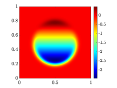
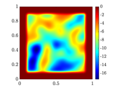
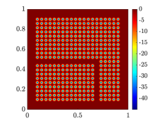
Figure 13. Lens (top left), random bumps (top right), and photonic crystal (bottom) scattering potentials.

	$N$	$h$	iter	res	$E_{\rm near}$	$E_{\rm far}$
Lens	102400	0.003125	51	6.38e-11	1.27e-02	2.06e-03
	409600	0.015625	9	6.18e-11	1.05e-05	6.77e-07
	1638400	0.00078125	7	4.86e-12	1.14e-08	5.22e-10
	6553600	0.000390625	7	7.64e-12	8.29e-11	2.81e-10
	26214400	0.0001953125	9	5.41e-12	7.85e-11	2.79e-10
Bumps	102400	0.003125	$100$	3.69e-02	3.14e-01	2.53e-02
	409600	0.015625	22	9.84e-11	3.90e-04	2.82e-04
	1638400	0.00078125	10	8.05e-12	4.17e-07	3.01e-07
	6553600	0.000390625	13	9.24e-11	5.29e-10	6.83e-10
	26214400	0.0001953125	23	3.71e-11	1.20e-10	9.90e-10
Crystal	102400	0.003125	24	6.49e-11	1.67e-03	1.09e-03
	409600	0.015625	8	3.70e-12	2.96e-06	1.47e-06
	1638400	0.00078125	7	2.30e-12	3.68e-09	1.29e-09
	6553600	0.000390625	15	2.24e-11	4.81e-10	2.94e-10
	26214400	0.0001953125	11	5.23e-11	4.57e-10	3.00e-10
Crystal 2	102400	0.003125	24	9.99e-11	5.15e-03	4.01e-03
	409600	0.015625	8	2.36e-12	7.12e-06	5.97e-06
	1638400	0.00078125	7	1.82e-12	7.88e-09	1.15e-08
	6553600	0.000390625	14	8.33e-11	1.67e-10	5.01e-09
	26214400	0.0001953125	11	4.75e-11	1.27e-10	5.00e-09

Table 11. Data for problems from [12] in Section 6.3.

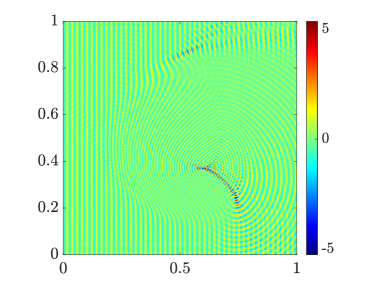
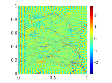
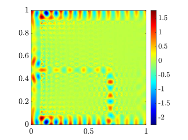
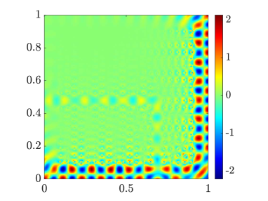
Figure 14. The real part of the total fields for the challenging problems from [12] in Section 6.3.

7. Conclusions

This paper describes an accelerated, high-order direct solver for the Lippmann-Schwinger equation for acoustic scattering. The solver is based on the Hierarchically Block Separable format, and specifically the formulation based on scattering matrices described in [5] and [20, Ch. 18]. We demonstrate that significant acceleration can be achieved by taking advantage of the particular form of the kernel function in this application, and of simplifications that arise from the use of uniform grids. The algorithm for computing an approximate inverse has asymptotic complexity $\mathcal{O}(N^{3/2})$, while applying the inverse has complexity $\mathcal{O}(N\log N)$.

Numerical experiments substantiate the claims in regards to the asymptotic complexity and demonstrate very favorable practical performance. A particularly effective method results from using the direct solver as a preconditioner for GMRES, with numerical experiments showing how a highly ill-conditioned cavity problem that is 500 wavelengths across can be solved to ten accurate digits in a couple of hours on a single workstation, using 26M degrees of freedom.

The specific direct solver described here is designed primarily for handling highly ill-conditioned problems in the high-frequency scattering regime. In this environment, the asymptotic complexities reported match those of existing state of the art solvers when the number of points per wavelength is fixed as the problem size $N$ is increased. Ongoing work is concerned with accelerating the solver to attain linear complexity in the situation where the elliptic PDE either has non-oscillatory solutions, or where the PDE is kept fixed as the problem size is increased, cf. Remark 4.2.

Acknowledgments

Vladimir Rokhlin has generously shared his insights about the problems under consideration, and we gratefully acknowledge his contributions. We thank Ran Duan for sharing codes to compute the quadrature weights, and Alex Barnett for sharing codes to compute the photonic crystal. The work of PGM was funded by the Office of Naval Research (award N00014-18-1-2354), by the National Science Foundation (awards 1952735 and 1620472), and by Nvidia Corp.

References

- [1] Sivaram Ambikasaran and Eric Darve. An fast direct solver for partial hierarchically semi-separable matrices. Journal of Scientific Computing, 57(3):477–501, 2013.
- [2] Ivo Babuška and Stefan Sauter. Is the pollution effect of the FEM avoidable for the Helmholtz equation considering high wave numbers? SIAM Journal on Numerical Analysis, 34(6):2392–2423, 1997.
- [3] Jean-Pierre Berenger. A perfectly matched layer for the absorption of electromagnetic waves. Journal of Computational Physics, 114(2):185–200, 1994.
- [4] Steffen Börm. Efficient numerical methods for non-local operators: -matrix compression, algorithms and analysis, volume 14. European Mathematical Society, 2010.
- [5] James Bremer, Adrianna Gillman, and Per-Gunnar Martinsson. A high-order accurate accelerated direct solver for acoustic scattering from surfaces. BIT Numerical Mathematics, 55(2):367–397, 2015.
- [6] Shivkumar Chandrasekaran and Ming Gu. A divide-and-conquer algorithm for the eigendecomposition of symmetric block-diagonal plus semiseparable matrices. Numerische Mathematik, 96(4):723–731, 2004.
- [7] Hongwei Cheng, Zydrunas Gimbutas, Per-Gunnar Martinsson, and Vladimir Rokhlin. On the compression of low rank matrices. SIAM Journal of Scientific Computing, 26(4):1389–1404, 2005.
- [8] David Colton and Rainer Kress. Inverse acoustic and electromagnetic scattering theory, volume 93. Springer Science & Business Media, 2012.
- [9] Eduardo Corona, Per-Gunnar Martinsson, and Denis Zorin. An direct solver for integral equations on the plane. Applied and Computational Harmonic Analysis, 38(2):284–317, 2015.
- [10] Ran Duan and Vladimir Rokhlin. High-order quadratures for the solution of scattering problems in two dimensions. Journal of Computational Physics, 228(6):2152–2174, 2009.
- [11] Björn Engquist and Andrew Majda. Absorbing boundary conditions for numerical simulation of waves. Proceedings of the National Academy of Sciences, 74(5):1765–1766, 1977.
- [12] Adrianna Gillman, Alex Barnett, and Per-Gunnar Martinsson. A spectrally accurate direct solution technique for frequency-domain scattering problems with variable media. BIT Numerical Mathematics, 55(1):141–170, 2015.
- [13] Adrianna Gillman, Patrick Young, and Per-Gunnar Martinsson. A direct solver with complexity for integral equations on one-dimensional domains. Frontiers of Mathematics in China, 7(2):217–247, 2012.
- [14] Leslie Greengard and Vladimir Rokhlin. A fast algorithm for particle simulations. Journal of Computational Physics, 73(2):325–348, 1987.
- [15] Leslie Greengard and Vladimir Rokhlin. On the numerical solution of two-point boundary value problems. Communications on Pure and Applied Mathematics, 44(4):419–452, 1991.
- [16] Ming Gu and Stanley Eisenstat. Efficient algorithms for computing a strong rank-revealing QR factorization. SIAM Journal on Scientific Computing, 17(4):848–869, 1996.
- [17] Wolfgang Hackbusch. A sparse matrix arithmetic based on -matrices. part I: Introduction to -matrices. Computing, 62(2):89–108, 1999.
- [18] Kenneth Ho and Leslie Greengard. A fast direct solver for structured linear systems by recursive skeletonization. SIAM Journal on Scientific Computing, 34(5):A2507–A2532, 2012.
- [19] Kenneth Ho and Lexing Ying. Hierarchical interpolative factorization for elliptic operators: Integral equations. Communications on Pure and Applied Mathematics, 69:1314–1353, 2016.
- [20] Per-Gunnar Martinsson. Fast Direct Solvers for Elliptic PDEs, volume CB96 of CBMS-NSF conference series. SIAM, 2019.
- [21] Per-Gunnar Martinsson and Vladimir Rokhlin. A fast direct solver for boundary integral equations in two dimensions. Journal of Computational Physics, 205(1):1–23, 2005.
- [22] Eric Michielssen, Amir Boag, and Weng Cho Chew. Scattering from elongated objects: direct solution in operations. IEE Proceedings - Microwaves, Antennas, and Propagation, 143(4):277 – 283, 1996.
- [23] Victor Minden, Kenneth Ho, Anil Damle, and Lexing Ying. A recursive skeletonization factorization based on strong admissibility. Multiscale Modeling & Simulation, 15(2):768–796, 2017.
- [24] Page Starr and Vladimir Rokhlin. On the numerical solution of two-point boundary value problems. II. Communications on Pure and Applied Mathematics, 47(8):1117–1159, 1994.
- [25] Franco Woolfe, Edo Liberty, Vladimir Rokhlin, and Mark Tygert. A fast randomized algorithm for the approximation of matrices. Applied and Computational Harmonic Analysis, 25(3):335–366, 2008.
- [26] Jianlin Xia, Shivkumar Chandrasekaran, Ming Gu, and Xiaoye S. Li. Fast algorithms for hierarchically semiseparable matrices. Numerical Linear Algebra with Applications, 17(6):953–976, 2010.