Single active particle engine utilizing a non-reciprocal coupling between particle’s position and self-propulsion

Abstract

We recently argued that a self-propelled particle is formally equivalent to a system consisting of two subsystems coupled by a non-reciprocal interaction [Phys. Rev. E 100, 050603(R) (2019)]. Here we show that this non-reciprocal coupling allows to extract useful work from a single self-propelled particle maintained at constant temperature, by using an aligning interaction to influence correlations between the particle’s position and self-propulsion.

Introduction. – During the last decade, active matter has attracted a lot of interest Ramaswamyrev1 ; Catesrev ; Marchettirev1 ; Bechingerrev ; Ramaswamyrev2 ; Marchettirev2 . The work in this area started with computer simulations of simple models and the postulation and analysis of active fluid’s hydrodynamics. Next, it transitioned to the development of statistical mechanical description of model active matter systems, typically consisting of the so-called self-propelled particles, i.e. particles that use the energy from their environment to move systematically. Very recently, a slightly different class of model systems, consisting of objects exhibiting non-reciprocal interactions that originate from some kind of activity, has become recognized for their unusual properties Brandenbourger ; Vitelli2020 .

Both assemblies of self-propelled particles and systems exhibiting non-reciprocal interactions can be used to construct engines that extract useful work while maintained at constant temperature. Proposals in the area of self-propelled particles include autonomous engines in which active particles power microscopic gears Sokolov ; DiLeonardo2010 ; DiLeonardo2017 or push asymmetric obstacles Pietzonka2019 and a cyclic engine that extracts work by changing the properties of the confining walls Ekeh . Notably, while proposed engines work due to the activity, they used its presence somewhat indirectly. In contrast, engine protocols that emerged in the area of materials with non-reciprocal interactions Vitelli2020 involve direct manipulation of the degree of freedom involved in non-reciprocal interactions, which then results in useful work done by the non-reciprocal force.

We argued recently Szamel2019 that a single self-propelled particle can be viewed as a system consisting of two subsystems coupled by a non-symmetric (violating Newton’s 3rd law), i.e. non-reciprocal interaction. This suggests a possibility to extract useful work from a single self-propelled particle by controlling directly the degree of freedom involved in the non-reciprocal interaction, i.e the self-propulsion. Specifically, we propose the following cyclic engine. If the particle’s self-propulsion is preferentially oriented towards the wall, the wall potential can be relaxed resulting in useful work obtained from the particle pushing on the wall. Then, if the direction of the self-propulsion can be reversed, the wall potential can be strengthen back to its original state. While it seems plausible that useful work would be done by the self-propulsion during the relaxing/re-strengthening parts of the cycle, the overall work balance depends also on the energetic cost of creating specific, atypical states of the self-propulsion orientation. Thus, a quantitative analysis of the proposed cycle’s performance is needed. We use the framework developed recently by Ekeh et al. Ekeh and show that useful work can indeed be extracted.

In the following we first discuss a model that can be partially analyzed analytically. It consists of a single active particle endowed with self-propulsion evolving according to the Ornstein-Uhlenbeck stochastic process, i.e. an active Ornstein-Uhlenbeck particle (AOUP) Szamel2014 ; Maggi2015 ; Fodor2016 , in a harmonic potential. The model used here is different from that introduced in Ref. Szamel2014 in that in addition to the self-propulsion there is also a thermal noise and an additional aligning interaction that controls the correlations between the self-propulsion and the position of the particle. For this model it can be shown analytically that useful quasistatic work can be extracted from the proposed cycle. Next, we use computer simulations to analyze a single active particle with self-propulsion of a constant magnitude and a freely-rotating direction, i.e. an active Brownian particle (ABP) tenHagen ; FilyMarchetti . The particle is moving in two spatial dimensions, under the influence of a harmonic potential and an aligning interaction controlling the correlations between the self-propulsion direction and the direction away from the center of the potential. In this case, computer simulation results show that useful work can be extracted from the proposed cycle.

Simple model engine: an AOUP in a harmonic potential. – The equations of motion for the position and the self-propulsion of the particle read,

$$\gamma\dot{x} =\!\!\!\!\!\underbrace{f}_{\text{non-recip.}}\!\!\!\!\!-kx-n\frac{\tau_{p}}{\gamma}f+\zeta \left<\zeta(t)\zeta(t^{\prime})\right>=2\gamma T\delta(t-t^{\prime})$$ (1)

$$\tau_{p}\dot{f} =-f-nx+\eta \left<\eta(t)\eta(t^{\prime})\right>=2\gamma T_{a}\delta(t-t^{\prime}).$$ (2)

In Eq. (1) $\gamma$ is the friction coefficient, $x$ is the position of the particle, $f$ is the self-propulsion and $n$ is the coupling constant quantifying the strength of an aligning interaction between the position and the self-propulsion. The aligning interaction controls the correlations between these two quantities. Its specific form was chosen to allow for analytical analysis of quasistatic cycles. Finally, $\zeta$ is the thermal white noise characterized by temperature $T$ (note that throughout the paper we use units such that $k_{B}=1$). In Eq. (2) $\tau_{p}$ is the persistence time of the self-propulsion and $\eta$ is the noise of the reservoir coupled to the self-propulsion, characterized by active temperature $T_{a}$. The first term at the right-hand-side (RHS) of Eq. (1) is the non-reciprocal term. This term induces non-trivial correlations between particle’s position and self-propulsion even in the absence of the aligning interaction characterized by coefficient $n$.

Without the non-reciprocal term in Eq. (1) and at the temperature equal to the active temperature, $T=T_{a}$, the system described by Eqs. (1-2) is equivalent to two harmonic oscillators coupled by an interaction term proportional to $n$, in contact with a heat reservoir at temperature $T$. Using the Fokker-Planck equation corresponding to Eqs. (1-2) one can show that the stationary, i.e. the equilibrium probability distribution is given by $p_{\text{eq}}(x,f)\propto\exp[-(kx^{2}/2+n\tau_{p}fx/\gamma+\tau_{p}f^{2}/(2\gamma))/T]$. In this case, quasistatic cycles defined by changing force constant $k$ and coupling constant $n$ produce no useful work in the surroundings and finite time cycles require external work to be performed on the system. It is instructive to note the role of the reciprocal coupling between position $x$ and self-propulsion $f$: for $n>0$, term $n\tau_{p}fx/\gamma$ induces negative cross-correlation between $x$ and $f$, $\left<xf\right>_{\text{eq}}<0$, where $\left<\ldots\right>_{\text{eq}}$ denotes averaging over the equilibrium ensemble.

The presence of the non-reciprocal term in Eq. (1) changes the system in a very profound way. To simplify the analysis we will consider only the case of the temperature equal to the active temperature, $T=T_{a}$. To analyze the work-dissipated heat balance we use the formalism developed by Ekeh et al. Ekeh We recognize that the quantity

$$u_{\text{tot}}(x,f)=\frac{1}{2}kx^{2}+n\frac{\tau_{p}}{\gamma}fx+\frac{1}{2}\frac{\tau_{p}}{\gamma}f^{2}$$ (3)

plays the role analogous to the total potential energy. This supposition is supported by the analysis of the mathematically equivalent system of two overdamped harmonic oscillators coupled by a reciprocal interaction characterized by $n$ and a non-reciprocal interaction that cannot be obtained from a potential. We consider a cyclic transformation driven by quasistatic changes of force constant $k$ and coupling coefficient $n$. Following Ekeh et al. we can write quasistatic work $W_{\text{qs}}$ as

$$W_{\text{qs}} = \oint_{\partial\Sigma}\left[\left<\frac{\partial u_{\text{tot}}}{\partial k}\right>_{\text{s}}dk+\left<\frac{\partial u_{\text{tot}}}{\partial u}\right>_{\text{s}}du\right]$$

$$= \pm\int\int_{\Sigma}\left[\frac{\partial}{\partial n}\left<\frac{\partial u_{\text{tot}}}{\partial k}\right>_{\text{s}}-\frac{\partial}{\partial k}\left<\frac{\partial u_{\text{tot}}}{\partial n}\right>_{\text{s}}\right]dkdn$$

In Eq. (Single active particle engine utilizing a non-reciprocal coupling between particle’s position and self-propulsion), $\partial\Sigma$ denotes the path in the $(k,n)$ plane defining the cyclic engine protocol and $\left<\ldots\right>_{\text{s}}$ denotes averaging over the stationary ensemble, which differs from the equilibrium ensemble due to the presence of the non-reciprocal term in Eq. (1). The second line of Eq. (Single active particle engine utilizing a non-reciprocal coupling between particle’s position and self-propulsion) is obtained using Green’s theorem; + and - signs refer to clockwise and counter-clockwise protocols $\partial\Sigma$, and $\Sigma$ denotes the part of the $(k,n)$ plane enclosed by $\partial\Sigma$.

For the present model stationary state averages $\left<\partial_{k}u_{\text{tot}}\right>_{\text{s}}=\left<x^{2}/2\right>_{\text{s}}$ and $\left<\partial_{n}u_{\text{tot}}\right>_{\text{s}}=\left<\tau_{p}xf/\gamma\right>_{\text{s}}$ can be calculated analytically,

$$\left<\frac{1}{2}x^{2}\right>_{\text{s}}=\frac{\tilde{T}}{2\tilde{k}}\left[1+\frac{\left(\tilde{n}-1\right)\left(\tilde{n}-1+\tilde{n}/\tilde{k}\right)}{\left(1+\tilde{k}\right)\left(1+\tilde{n}\left(1-\tilde{n}\right)/\tilde{k}\right)}\right],$$ (5)

$$\left<\frac{\tau_{p}}{\gamma}xf\right>_{\text{s}}=-\tilde{T}\frac{\tilde{n}-1+\tilde{n}/\tilde{k}}{\left(1+\tilde{k}\right)\left(1+\tilde{n}\left(1-\tilde{n}\right)/\tilde{k}\right)},$$ (6)

where $\tilde{T}=T\tau_{p}/\gamma$, $\tilde{k}=k\tau_{p}/\gamma$ and $\tilde{n}=n\tau_{p}/\gamma$. A direct inspection shows that the integrand in the second line of Eq. (Single active particle engine utilizing a non-reciprocal coupling between particle’s position and self-propulsion) $w_{\text{qs}}=\partial_{n}\left<\partial_{k}u_{\text{tot}}\right>_{\text{s}}-\partial_{k}\left<\partial_{n}u_{\text{tot}}\right>_{\text{s}}\neq 0$ and thus a non-vanishing useful quasistatic work can be extracted from a cyclic process in the $(k,n)$ plane.

For illustration, we considered the following cycle in the $(k\tau_{p}/\gamma,n\tau_{p}/\gamma)$ plane: $(1,-.5)\rightarrow(1,.5)\rightarrow(2,.5)\rightarrow(2,-.5)\rightarrow(1,-.5)$. In the part of the $(k,n)$ plane enclosed by this cycle integrand $w_{\text{qs}}$ does not change the sign, which allows us to vary $k$ and $n$ independently Ekeh . We obtained quasitatic work $W_{\text{qs}}=0.545\,T$.

Next, we consider finite-time cycles. We note that the average of finite-time work $W$,

$$W=\int_{0}^{\tau_{c}}\left[\frac{\partial u_{\text{tot}}}{\partial k}\dot{k}+\frac{\partial u_{\text{tot}}}{\partial n}\dot{n}\right]dt$$ (7)

can be expressed in terms of the moments of the time-dependent probability distribution. Specifically, to evaluate $\left<W\right>_{t}$ we need $\left<x^{2}/2\right>_{t}$ and $\left<\tau_{p}xf/\gamma\right>_{t}$. Here $\left<\dots\right>_{t}$ denotes averaging over time-dependent probability distribution that can be obtained by solving the Fokker-Planck equation corresponding to equations of motion (1-2), with time-dependent couplings $k(t)$ and $n(t)$. Since Eqs. (1-2) are linear, equations of motion for second moments do not involve higher moments. We obtain the following equations of motion for three second moments,

$$\frac{\partial}{\partial t}\left<\frac{1}{2}x^{2}\right>_{t}\!\!\! = \!-2\frac{k(t)}{\gamma}\left<\frac{1}{2}x^{2}\right>_{t}+\frac{T}{\gamma}$$ (8)

$$\!\!\!\!\!+\left(\frac{1}{\tau_{p}}-\frac{n(t)}{\gamma}\right)\left<\frac{\tau_{p}}{\gamma}xf\right>_{t}$$

$$\frac{\partial}{\partial t}\left<\frac{\tau_{p}}{\gamma}xf\right>_{t}\!\!\! = \!-\left(\frac{k(t)}{\gamma}+\frac{1}{\tau_{p}}\right)\left<\frac{\tau_{p}}{\gamma}xf\right>_{t}$$

$$\!\!\!\!\!-2\frac{n(t)}{\gamma}\left<\frac{1}{2}x^{2}\right>_{t}+2\left(\frac{\tau_{p}}{\gamma^{2}}-\frac{n\tau_{p}^{2}}{\gamma^{3}}\right)\left<\frac{1}{2}f^{2}\right>_{t}$$

$$\frac{\partial}{\partial t}\left<\frac{1}{2}f^{2}\right>_{t}\!\!\! = \!-\frac{2}{\tau_{p}}\left<\frac{1}{2}f^{2}\right>_{t}+\frac{T\gamma}{\tau_{p}^{2}}$$ (10)

$$\!\!\!\!\!-\frac{n(t)\gamma}{\tau_{p}^{2}}\left<\frac{\tau_{p}}{\gamma}xf\right>_{t}.$$

Eqs. (8-10) were solved numerically numdiff for the same cycle for which we calculated the quasistatic work; in the $(k\tau_{p}/\gamma,n\tau_{p}/\gamma)$ plane the cycle reads $(1,-.5)\rightarrow(1,.5)\rightarrow(2,.5)\rightarrow(2,-.5)\rightarrow(1,-.5)$, with $k(t)$ and $n(t)$ changing linearly with time in elements 2 and 4 and 1 and 3 of the cycle, respectively. Cycle time dependence of the resulting average useful work (work done in the surroundings) $-\left<W\right>_{t}$ and power $\left<\mathcal{P}\right>_{t}\equiv-\left<W\right>_{t}/\tau_{c}$ are shown in Figs. 1(a)-1(b). We find that the results are similar to those of Ekeh et al. Ekeh : useful work is extracted only for long enough cycles and power reaches its peak value for an intermediate cycle time.

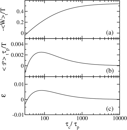
Figure 1: Dependence of the thermodynamic quantities characterizing the AOUP engine on the cycle time scaled by the persistence time, $\tau_{c}/\tau_{p}$. (a) Average useful work normalized by the temperature, $-\left<W\right>_{t}/T$. (b) Average power normalized by the ratio of the temperature and the persistence time, $\left<\mathcal{P}\right>_{t}/(T/\tau_{p})$. (c) Engine efficiency $\mathcal{E}$.

To evaluate efficiency of the cycle we extend the formalism of Ekeh et al. to the present case of an AOUP engine. Briefly, we define heat as work done on the two subsystems by their respective thermostats,

$$Q=\int_{0}^{\tau_{c}}\left[\left(\gamma\dot{x}-\zeta\right)\dot{x}+\frac{\tau_{p}}{\gamma}\left(\tau_{p}\dot{f}-\eta\right)\dot{f}\right]dt.$$ (11)

Again, expression (11) can be justified by analyzing the mathematically equivalent system of two coupled harmonic oscillators. Following Ekeh et al. we find that

$$\left<Q\right>_{t}=\left<W\right>_{t}+\int_{0}^{\tau_{c}}f\dot{x}dt,$$ (12)

which allows us to calculate the efficiency,

$$\mathcal{E}=\frac{-\left<W\right>_{t}}{-\left<W\right>_{t}+\left<Q\right>_{t}}$$ (13)

In Fig. 1(c) we show the cycle time dependence of the efficiency. Again, our results are qualitatively similar to those of Ekeh et al. Ekeh : the efficiency reaches its peak value for an intermediate cycle time, close to the cycle time corresponding to the peak value of the power. We note that the efficiency of our simple single AOUP engine is several orders of magnitude larger that that of the engine analyzed in Ref. Ekeh .

An ABP engine. – The equations of motion for a single active Brownian particle moving in a two-dimensional harmonic potential and subjected to an additional aligning interaction read,

$$\gamma_{t}\dot{\mathbf{r}} =\!\!\!\underbrace{\gamma_{t}v_{0}\mathbf{e}}_{\text{non-recip.}}\!\!\!-\partial_{\mathbf{r}}u_{\text{tot}}+\boldsymbol{\zeta} \left<\boldsymbol{\zeta}(t)\boldsymbol{\zeta}(t^{\prime})\right>=2\boldsymbol{I}\gamma_{t}T\delta(t-t^{\prime}),$$ (14)

$$\gamma_{r}\dot{\varphi} =-\partial_{\varphi}u_{\text{tot}}+\eta \left<\eta(t)\eta(t^{\prime})\right>=2\gamma_{r}T\delta(t-t^{\prime}).$$ (15)

In Eqs. (14-15) $\gamma_{t}$ and $\gamma_{r}$ is the translational and rotational friction constant, respectively and $\boldsymbol{I}$ is a unit two-dimensional tensor. Furthermore, $\mathbf{e}\equiv(\cos(\varphi),\sin(\varphi))$ is the orientation vector specifying the direction of the self-propulsion and $u_{\text{tot}}$ denotes the total potential energy, which is a sum of the harmonic and aligning contributions, $u_{\text{tot}}(\mathbf{r},\varphi)=k\mathbf{r}^{2}/2+l\hat{\mathbf{r}}\cdot\mathbf{e}$. We note that the coefficients characterizing the strength of the aligning interaction for the AOUP and ABP systems have different dimensions and for this reason we use different symbols to refer to them. Finally, $\boldsymbol{\zeta}$ and $\eta$ are thermal white noises characterized by temperature $T$. We recall that the orientational dynamics of ABPs is often discussed in terms of rotational diffusion coefficient $D_{r}=T/\gamma_{r}$, which physically corresponds to the inverse of the persistence time of AOUPs. The first term at the RHS of Eq. (14) is the non-reciprocal term. Its magnitude is quantified by self-propulsion velocity $v_{0}$. As for the AOUP, the non-

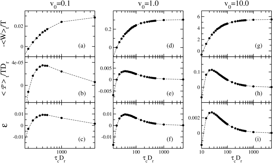
Figure 2: Dependence of the thermodynamic quantities characterizing the ABP engine on the cycle time scaled by the rotational diffusion coefficient, $\tau_{c}D_{r}$, for self-propulsion velocity $v_{0}=0.1$ (left panels), $v_{0}=1.0$ (middle panels) and $v_{0}=10.0$ (right panels). (a,d,g) Average useful work normalized by the temperature, $-\left<W\right>_{t}/T$. (b,e,h) Average power normalized by the product of the temperature and the rotational diffusion coefficient, $\left<\mathcal{P}\right>_{t}/(TD_{r})$. (c,f,i) Engine efficiency $\mathcal{E}$.

reciprocal term induces non-trivial correlations between particle’s position and orientation, even in the absence of the aligning interaction.

To analyze the single ABP engine we solved Eqs. (14-15) numerically numsol with time-dependent couplings $k(t)$ and $l(t)$ following a cycle similar to that used for the single AOUP engine. Specifically, in the $(k/(\gamma_{t}D_{r}),l/T)$ plane we considered path $(1,-1)\rightarrow(1,1)\rightarrow(2,1)\rightarrow(2,-1)\rightarrow(1,-1)$, with $k(t)$ and $l(t)$ changing linearly with time in elements 2 and 4 and 1 and 3 of the cycle, respectively. We note that for the single ABP engine the magnitude of the self-propulsion velocity is an additional parameter, which can be varied for a given cycle path.

In Fig. 2 we show average useful work $-\left<W\right>_{t}$, power $-\left<W\right>_{t}/\tau_{c}$ and efficiency $\mathcal{E}$, calculated in the same way as for the single AOUP engine, for a range of the cycle times and three self-propulsion velocities, $v_{0}=0.1$, 1.0 and 10. Qualitatively, for any $v_{0}$ the results are similar to those for the single AOUP engine. The main trends are increasing magnitude of both the useful work and the maximum power with increasing $v_{0}$, decreasing efficiency for larger $v_{0}$ and decreasing the cycle time at which the maximum power and efficiency are attained with increasing $v_{0}$.

Discussion. – We have proposed a general framework for simple engines utilizing the non-reciprocal interaction that is inherent in many active particles’ models. We have analyzed two examples of such engines, that use as working bodies single self-propelled particles. We have shown that by manipulating correlations between particle’s position and self-propulsion one can extract useful work from monothermal cycles. Generally, these engines achieve maximum power and maximum efficiency for finite time cycles.

We note that our framework can be further simplified: it should be possible to extract useful work from a single self-propelled particle engine using a feedback mechanism based on periodic observation of the self-propulsion direction. If the direction is pointing towards the wall, the wall potential can be relaxed and, conversely, if the direction is pointing towards the center of the potential, the wall potential can be re-strengthen. This new framework resembles a continuous Maxwell demon proposed, analyzed and experimentally realized by Ribezzi-Crivellari and Ritort Ribezzi . Its quantitative analysis requires taking into account thermodynamic aspects of the information content ParrondoHorowitzSagawa and is left for a future study.

- (1) S. Ramaswamy, “The Mechanics and Statistics of Active Matter”, Ann. Rev. Condens. Matter Phys. 1, 323 (2010).
- (2) M.E. Cates, “Diffusive transport without detailed balance in motile bacteria: does microbiology need statistical physics?”, Rep. Prog. Phys. 75, 042601 (2012).
- (3) M.C. Marchetti, J.F. Joanny, S. Ramaswamy, T.B. Liverpool, J. Prost, M. Rao, and R.A. Simha, “Hydrodynamics of soft active matter”, Rev. Mod. Phys. 85, 1143 (2013).
- (4) C. Bechinger, R. Di Leonardo, H. Löwen, C. Reichhardt, G. Volpe and G. Volpe, “Active particles in complex and crowded environments”, Rev. Mod. Phys. 88, 045006 (2016).
- (5) S. Ramaswamy, “Active matter”, J. Stat. Mech. 054002 (2017).
- (6) E. Fodor and M.C. Marchetti, “The statistical physics of active matter: From self-catalytic colloids to living cells”, Physica A 504, 106 (2018).
- (7) M. Brandenbourger, X. Locsin, E. Lerner and C. Coulais, “Non-reciprocal robotic metamaterials”, Nature Communications 10, 4607 (2019).
- (8) C. Scheibner, A. Souslov, D. Banerjee, W.T.M. Irvine and V. Vitelli, “Odd elasticity”, Nature Physics 16, 475 (2020).
- (9) A. Sokolov, M. M. Apodaca, B. A. Grzybowski, and I.S. Aranson, “Swimming bacteria power microscopic gears”, Proc. Natl. Acad. Sci. USA 107, 969 (2010).
- (10) R. Di Leonardo, L. Angelani, D. Dell’Arciprete, G. Ruocco, V. Iebba, S. Schippa, M.P. Conte, F. Mecarini, F. De Angelis, and E. Di Fabrizio, “Bacterial ratchet motors”, Proc. Natl. Acad. Sci. USA 107, 9541 (2010).
- (11) G. Vizsnyiczai, G. Frangipane, C. Maggi, F. Saglimbeni, S. Bianchi, and R. Di Leonardo, “Light controlled 3D micromotors powered by bacteria”, Nature Communications 8, 15974 (2017).
- (12) P. Pietzonka, E. Fodor, C. Lohrmann, M.E. Cates, and U. Seifert, “Autonomous Engines Driven by Active Matter: Energetics and Design Principles”, Phys. Rev. X 9, 041032 (2019).
- (13) T. Ekeh, M.E. Cates, and E. Fodor, “Thermodynamic cycles with active matter”, Phys. Rev. E 102, 010101(R) (2020).
- (14) G. Szamel, “Stochastic thermodynamics for self-propelled particles”, Phys. Rev. E 100, 050603(R) (2019).
- (15) G. Szamel, “A self-propelled particle in an external potential: Existence of an effective temperature”, Phys. Rev. E 90, 012111 (2014).
- (16) C. Maggi, U.M.B. Marconi, N. Gnan, and R. Di Leonardo, “Multidimensional stationary probability distribution for interacting active particles”, Scientific Reports 5, 10742 (2015).
- (17) E. Fodor, C. Nardini, M. E. Cates, J. Tailleur, P. Visco, and F. van Wijland, “How Far from Equilibrium Is Active Matter?”, Phys. Rev. Lett. 117, 038103 (2016).
- (18) B. ten Hagen, S. van Teeffelen and H. Löwen, “Brownian motion of a self-propelled particle”, J. Phys.: Condens. Matter 23 194119 (2011).
- (19) Y. Fily and M.C. Marchetti, “Athermal Phase Separation of Self-Propelled Particles with No Alignment”, Phys. Rev. Lett. 108, 235702 (2012)
- (20) We used fourth-order Runge-Kutta routine rk4; see W.H. Press, S.A. Teukolsky, W.T. Vetterling and B.P. Flannery, Numerical Recipes in FORTRAN, 2nd ed. (Cambridge University Press, New York, 1992).
- (21) We used the Euler-Maruyama method with time step and averaged over at least realizations.
- (22) M. Ribezzi-Crivellari and F. Ritort, “Large work extraction and the Landauer limit in a continuous Maxwell demon”, Nature Physics 15, 660 (2019).
- (23) J.M.R. Parrondo, J.M. Horowitz and T. Sagawa, “Thermodynamics of information”, Nature Physics 11, 131 (2015).