Lessons on Star-forming Ultra-diffuse Galaxies from The Stacked Spectra of Sloan Digital Sky Survey

Abstract

We investigate the on-average properties for 28 star-forming ultra-diffuse galaxies (UDGs) located in low-density environments, by stacking their spectra from the Sloan Digital Sky Survey. These relatively-isolated UDGs, with stellar masses of $\log_{10}(M_{*}/M_{\odot})\sim 8.57\pm 0.29$, have the on-average total-stellar-metallicity [M/H]$\sim-0.82\pm 0.14$, iron-metallicity [Fe/H]$\sim-1.00\pm 0.16$, stellar age $t_{*}\sim 5.2\pm 0.5$ Gyr, $\alpha$-enhancement [$\alpha$/Fe]$\sim 0.24\pm 0.10$, and oxygen abundance 12+$\log$(O/H)$\sim 8.16\pm 0.06$, as well as central stellar velocity dispersion $54\pm 12$ km/s. On the star-formation rate versus stellar mass diagram, these UDGs are located lower than the extrapolated star-forming main sequence from the massive spirals, but roughly follow the main sequence of low-surface-brightness dwarf galaxies. We find that these star-forming UDGs are not particularly metal-poor or metal-rich for their stellar masses, as compared with the metallicity-mass relations of the nearby typical dwarfs. With the UDG data of this work and previous studies, we also find a coarse correlation between [Fe/H] and magnesium-element enhancement [Mg/Fe] for UDGs: [Mg/Fe]$\simeq-0.43(\pm 0.26)$[Fe/H]$-0.14(\pm 0.40)$.

1 Introduction

As a possible challenge to current galaxy formation models, many properties of the population of ultra-diffuse galaxies (UDGs; van Dokkum et al., 2015; Mihos et al., 2015), including but not limited to their halo masses and dark matter fractions (e.g., van Dokkum et al., 2016, 2018), spins (Rong et al., 2017a; Leisman et al., 2017), alignments and morphologies (e.g., Yagi et al., 2016; Rong et al., 2019a, b, 2020), gas content and star formation (e.g., Trujillo et al., 2017; Leisman et al., 2017), and particularly, metallicities (e.g., Gu et al., 2018; Ruiz-Lara et al., 2018; Ferré-Mateu et al., 2018; Pandya et al., 2018; Martín-Navarro et al., 2019; Fensch et al., 2019), are still not clear. To the present, the studies for UDG metallicities are almost focused on the quiescent members in galaxy clusters/groups; the metallicity properties of star-forming UDGs are barely investigated.

Metallicity is one of the fundamental observational quantities that could provide information about the evolution of UDGs. The metal content of a galaxy is determined by a complex interplay between cosmological gas inflow, metal production by stars, and gas outflow via feedback. Inflows usually dilute the metallicity of a galaxy (e.g., Rupke et al., 2010) while provide fuel for star formation, which then convert hydrogen and helium to heavier elements. The outflows driven by stellar or AGN feedback inject energy into the interstellar medium and flow the gas and metals out of the galaxy (e.g., Rong et al., 2017b; Christensen et al., 2018). The ejected metals can escape from the gravitational potential well of the galaxy or be re-accreted into the galaxy and enrich it again. Measuring the gas-phase and stellar metallicities thus augments the understanding of the importance of outflows/inflows during UDG formation. The studies of the $\alpha$-element enhancement of UDG stellar population can, however, provide clues about the time-scale of star formation in UDGs. The $\alpha$-enhancement is measured through the [$\alpha$/Fe] ratio, where $\alpha$-elements and irons (Fe) are ejected into the interstellar medium primarily by Type II and Ia supernovae (SN II and SN Ia), respectively. Since SN Ia start to occur $\sim 1$ Gyr after the onset of star formation while SN II appear much sooner, the ratio of $\alpha$ elements, such as magnesium to iron ([Mg/Fe]), can be used to estimate relative star-formation timescales. A shorter episode of star formation in a UDG will result in an $\alpha$-enhanced stellar population due to the enrichment of magnesium from the SN II, and the $\alpha$-enhancement will begin to drop after SN Ia appear due to the dilution of magnesium with iron in the interstellar medium (Thomas et al., 2005).

We will select a sample of star-forming UDGs with spectra from the Sloan Digital Sky Survey (SDSS), located in the low-density environments, and stack their spectra to obtain a relatively-high signal-to-noise ratio (S/N) spectrum, and then study the on-average metallicity with the stacked spectrum. In section 2, we will describe the selection of UDG sample. We will describe the method of stacking the spectra of UDGs and investigate the on-average UDG properties in section 3, as well as discuss our results in section 4. In this paper, we assume the Hubble constant $H_{0}=69.6$ km/s (Bennett et al., 2014), and use “log” to represent “$\log_{10}$”.

2 Selecting UDGs in SDSS

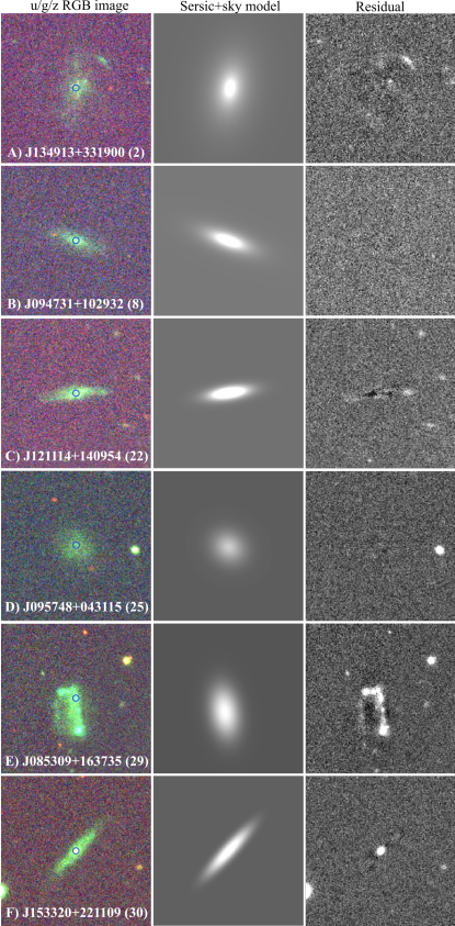
Figure 1: The left, middle, and right panels show the original RGB images, fitting models, and residuals ($g$-band), respectively. Panels A, B, C, and D show the examples of the selected UDGs in this work; panels E and F exhibit the two abandoned UDG candidates since the SDSS 3 arcsec spectroscopic fiber (blue circles in the left panels show the 3 arcsec aperture) targets at the star-forming region and central nucleus with the distinct color from the entire stellar body, respectively. The SDSS names of these galaxies are also shown in the corresponding panels; the numbers in the brackets correspond to the UDG numbers in Table 1.

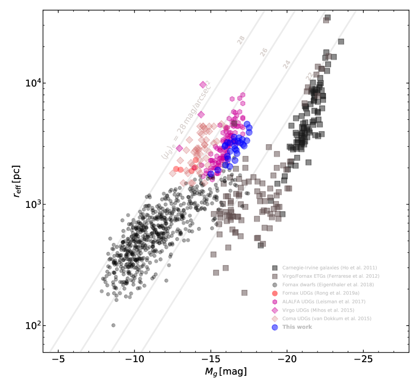
Figure 2: The scale relation for the UDGs in this work (blue filled circles), and UDGs in the Virgo (purple diamonds; Mihos et al., 2015), Coma (light-orange diamonds; van Dokkum et al., 2015), and Fornax (red filled circles; Rong et al., 2019a) clusters, as well as fields (purple hexagons; Leisman et al., 2017), plotted on that of typical dwarfs (black filled circles) and massive galaxies (squares) in the nearby clusters (Ho et al., 2011; Ferrarese et al., 2012).

We first select a sample of low-surface-brightness galaxies with the mean surface brightness (within effective radius $r_{\rm{eff}}$) $\langle\mu_{\rm{eff,abs}}(r)\rangle>22.5\ \rm{mag/arcsec^{2}}$ from the galaxy catalog of Simard et al. (2011), which contains 670,131 galaxies with SDSS optical spectra; each galaxy was roughly fitted with a pure Sérsic model by Simard et al. (2011); we only select the large galaxies with $r_{\rm{eff}}>1.5$ kpc as the candidates. The optical images of these candidates are then inspected by eyes to further abandon the objects being the substructures of large galaxies or having close companions such as bright stars or galaxies. 103 candidates are preliminarily selected.

For each selected candidate, we utilize a Sérsic+sky model to fit its $g$ and $r$-band fully-processed SDSS images with Galfit (Peng et al., 2010), by using the iterative fitting methodology outlined in Eigenthaler et al. (2018) (to remove the contaminations of member globular clusters, background interlopers, and star-forming regions, etc). In Fig. 1, we show the fitting results of several examples. The stellar masses are estimated by using the $r$-band luminosities and stellar mass-to-light ratios derived from the Galactic extinction corrected colors, $\log(M_{*}/L)=-0.306-0.15+1.097\times(g-r)$ (Guo et al., 2020). The 33 galaxies with the $g$-band central surface brightness $\mu_{0,g}>23.5\ \rm{mag/arcsec^{2}}$, $r_{\rm{eff}}>1.5$ kpc, and $\log M_{*}<9.0$ are selected as UDGs.

Among the 33 UDGs, there are 5 UDGs for which the SDSS $3^{\prime\prime}$ fiber aperture targeted at their star-forming regions (e.g., panel E of Fig. 1) or central nuclei/small-bulges (e.g., panel F of Fig. 1); these regions exhibit the colors significantly different from the colors of their entire stellar bodies in their RGB images. Therefore, the 5 UDGs are further abandoned, since their SDSS spectra cannot reveal the on-average properties of these UDGs. Finally, only 28 UDGs with SDSS spectra are selected, as listed in Table 1; each selected UDG resides in the low-density environment, i.e., outside of the virial radius ($R_{\rm{vir}}$) of the nearest galaxy group/cluster (Saulder et al., 2016). As explored in Fig. 2, our UDG sample represents the relatively-bright UDG population; it is because that our UDGs are star-forming (cf. Fig. 3), and thus have relatively-lower $M_{*}/L$ than those UDGs in clusters; therefore, the same $M_{*}$ range corresponds to relatively-brighter star-forming UDGs.

Num	RA	DEC	$z$	distance	$\mu_{0,g}$	$r_{\rm{eff}}$	$m_{r,\rm{f}}$	$M_{r}$	$g-r$	$\log M_{*}$	R/Rvir	SFRfiber	SFRtot
	(deg)	(deg)		(Mpc)	(mag/′′2)	(kpc)	(mag)	(mag)	(mag)	($\log M_{\odot}$)		($M_{\odot}$/yr)	($M_{\odot}$/yr)
1	164.087	56.760	0.00615	29.6	23.75	2.9	19.49	-17.14	0.56	8.9	1.83	$1.0\times 10^{-4}$	$6.1\times 10^{-3}$
2	207.304	33.317	0.00723	35.0	23.75	1.8	20.95	-15.32	0.31	7.9	5.37	$1.9\times 10^{-4}$	$6.4\times 10^{-3}$
3	232.685	47.319	0.00855	38.0	24.02	3.6	20.27	-17.07	0.54	8.8	2.93	$3.0\times 10^{-3}$	$1.4\times 10^{-1}$
4	185.314	58.085	0.00944	41.3	23.51	2.3	19.50	-17.02	0.43	8.7	8.60	$8.9\times 10^{-4}$	$2.3\times 10^{-2}$
5	234.388	58.580	0.00972	42.7	23.85	2.4	19.72	-16.58	0.45	8.5	1.28	$1.8\times 10^{-3}$	$3.2\times 10^{-2}$
6	111.809	42.204	0.01003	44.8	24.53	3.1	21.01	-16.46	0.51	8.5	3.45	$8.4\times 10^{-4}$	$3.1\times 10^{-2}$
7	234.284	20.146	0.01027	45.9	25.02	3.0	20.82	-16.19	0.26	8.2	4.96	$8.2\times 10^{-3}$	$1.6\times 10^{-1}$
8	146.881	10.492	0.01044	49.6	23.97	1.9	20.41	-15.75	0.29	8.0	1.74	$1.3\times 10^{-3}$	$2.0\times 10^{-2}$
9	177.654	24.926	0.01216	56.7	23.86	2.5	20.39	-16.35	0.27	8.2	1.80	$4.7\times 10^{-4}$	$8.1\times 10^{-3}$
10	146.339	14.580	0.01267	59.3	24.36	3.2	19.96	-16.59	0.33	8.4	5.75	$2.7\times 10^{-3}$	$3.5\times 10^{-2}$
11	139.232	14.714	0.01314	58.5	24.15	2.7	20.76	-16.64	0.36	8.4	8.37	$2.8\times 10^{-4}$	$7.7\times 10^{-3}$
12	48.454	-8.147	0.01372	56.8	23.68	2.8	19.66	-16.90	0.23	8.4	2.76	$9.6\times 10^{-3}$	$9.0\times 10^{-2}$
13	187.568	3.073	0.01366	63.9	23.66	2.1	19.93	-16.26	0.28	8.2	10.5	$2.6\times 10^{-3}$	$2.3\times 10^{-2}$
14	191.489	35.171	0.01453	68.2	24.00	3.3	19.95	-16.87	0.31	8.5	6.24	$2.3\times 10^{-3}$	$3.0\times 10^{-2}$
15	157.110	31.262	0.01497	69.0	23.56	2.0	20.26	-16.50	0.25	8.3	6.06	$3.3\times 10^{-3}$	$3.5\times 10^{-2}$
16	153.282	36.096	0.01491	69.0	24.72	3.2	20.41	-16.48	0.38	8.4	7.84	$1.3\times 10^{-3}$	$1.7\times 10^{-2}$
17	240.561	17.506	0.01589	70.4	24.00	3.4	20.29	-17.42	0.35	8.8	2.98	$1.4\times 10^{-3}$	$3.2\times 10^{-2}$
18	202.486	-0.614	0.01652	75.7	23.65	3.0	19.91	-17.54	0.35	8.8	6.39	$2.5\times 10^{-3}$	$3.6\times 10^{-2}$
19	121.914	56.925	0.01832	80.7	23.68	3.0	20.67	-17.02	0.45	8.7	6.41	$1.8\times 10^{-3}$	$3.1\times 10^{-2}$
20	152.880	65.090	0.02008	88.1	23.83	3.9	19.32	-17.86	0.34	8.9	13.7	$1.3\times 10^{-2}$	$1.2\times 10^{-1}$
21	197.298	28.777	0.02123	94.6	23.84	2.6	20.70	-17.06	0.34	8.6	2.28	$3.5\times 10^{-3}$	$4.5\times 10^{-2}$
22	182.807	14.165	0.02119	96.2	24.27	3.5	20.13	-17.31	0.46	8.8	6.73	$7.6\times 10^{-3}$	$6.3\times 10^{-2}$
23	171.122	34.581	0.02128	96.6	23.88	3.2	19.83	-17.34	0.39	8.8	1.80	$4.8\times 10^{-3}$	$4.1\times 10^{-2}$
24	176.358	32.252	0.02150	97.2	23.97	3.3	20.13	-17.18	0.39	8.7	5.47	$3.9\times 10^{-3}$	$3.5\times 10^{-2}$
25	149.448	4.521	0.02137	99.4	23.90	3.1	20.84	-17.55	0.43	8.9	9.87	$1.3\times 10^{-3}$	$2.8\times 10^{-2}$
26	177.310	36.763	0.02196	98.4	24.29	4.6	19.87	-17.66	0.28	8.8	6.77	$5.7\times 10^{-3}$	$6.5\times 10^{-2}$
27	256.171	62.035	0.02324	99.8	23.75	4.3	19.84	-17.85	0.33	8.9	15.8	$1.4\times 10^{-2}$	$1.4\times 10^{-1}$
28	166.879	16.755	0.02665	120.0	23.57	3.4	19.93	-17.72	0.35	8.9	10.2	$5.2\times 10^{-3}$	$4.5\times 10^{-2}$

Table 1: Properties of the selected UDGs. Col. (1): galaxy number; Col. (2): RA; Col. (3): DEC; Col. (4): spectroscopic redshift; Col. (5): distance to us (corrected for CMB), obtained from the NASA/IPAC Extragalactic Database; Col. (6): observed $g$-band central surface brightness; Col. (7): $g$-band effective radius; Col. (8): $r$-band SDSS fiberMag without correction for extinction; Col. (9): $r$-band absolute magnitude corrected for Galactic extinction; Col. (10): $g-r$ color corrected for Galactic extinction; Col. (11): estimated stellar mass; Col. (12): three-dimensional distance to the nearest galaxy cluster/group, normalized by the virial radius of group/cluster; Col. (13): SFR covered by the SDSS $3^{\prime\prime}$ fiber aperture; Col. (14): estimated total star-formation rate.

3 Data analysis and UDG properties

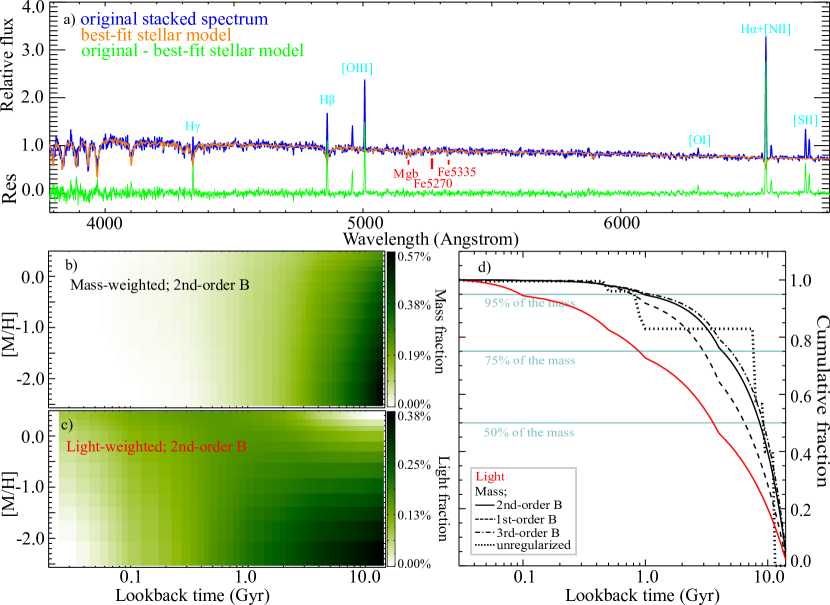
Figure 3: Panel a: the stacked spectrum (blue), best-fit stellar model (orange), and residual (green) of the selected 28 UDGs. The Mg-feature, Mgb, and Fe-features, Fe5270 & Fe5335, are also shown. Panels b & c show the regularized (with the 2nd-order regularization matrix) mass-weighted and light-weighted stellar age-metallicity distributions revealing SFH, respectively, with the color-bars giving the mass and light fractions corresponding to each value for age and metallicity. Panel d: the mass assembly (black) and light assembly (red) of our UDGs; the dark-green lines indicate when our UDGs had already formed 50%, 75%, and 95% of their stellar masses/light, respectively. For comparison, we show the SFH without regularization (dotted) as well as SFHs with the regularized solutions of applying the first- (dashed), second- (solid), and third-order (dot-dashed) regularization matrix $\bm B$, i.e., $\bm B$=diag(1,-1), $\bm B$=diag(1,-2,1), and $\bm B$=diag(1,-3,3,-1), respectively (cf. Boecker et al., 2020).

Since the S/N (defined as the median S/N in 5490-5510 Å) of an individual UDG spectrum is low (S/N$\sim 3\--14$), we stack the spectra of the selected UDGs and study the on-average stellar and gas-phase metallicities. For each galaxy spectrum from SDSS, we first correct it for the Galactic extinction by using the extinction curve of Fitzpatrick (1999) with $R_{V}=3.1$ and $E(B-V)$ value from the NASA/IPAC Extragalactic Database; the spectrum is then shifted to the rest frame and interpolated onto a wavelength grid spanning $3790\-–6800\AA$ with spacing $\Delta\ln\lambda\ (\AA)=1$. Each spectrum is normalized with the median flux density in $4400\--4450\AA$. We then stack the spectra using the median flux density at each wavelength (S/N$\sim 30$ for the stacked spectrum); the stacked spectrum is shown in Fig. 3. The significant H$\alpha$ emission line indicates that our relatively-isolated UDGs are star-forming.

Since the old stellar population would be shaded by the light of the recently-formed stars in our star-forming UDGs, in order to study the star-formation history (SFH) and mass-weighted properties for our UDGs, analogous to the work of Fahrion et al. (2019) and Rong et al. (2018), we use pPXF (Cappellari, 2017, V7.3.0) to fit the stacked spectrum, with the MILES single stellar population (SSP) template spectra (Vazdekis et al., 2015), plus emission-line models (assuming the Balmer decrement for Case B recombination). The MILES models implement the BaSTI isochrones (Pietrinferni et al., 2006) and a Milky Way-like, double power law (bimodal), initial mass function (IMF) with a high mass slope of 1.30, and include 53 ages from 30 Myr to 14 Gyr, and 12 stellar metallicities from [M/H]=-2.27 to +0.40. We follow the linear regularization process of (McDermid et al., 2015, adopting the second-order regularization matrix, i.e., the pPXF option ‘REG_ORD’=2) to smooth the variation in the weights of templates of similar ages and metallicities. Since the original MILES library only offers the scaled solar models ([$\alpha$/Fe]=0) and alpha enhanced models ([$\alpha$/Fe]=0.4 dex), using a regularized pPXF solution seems unphysical; to develop a better sampled grid of SSP models for the fits, we linearly interpolate between the available SSPs to create a grid from [$\alpha$/Fe]=0 to [$\alpha$/Fe]=0.4 dex with a spacing of 0.1 dex, following the same method described in Fahrion et al. (2019). These models are created under the assumption that the [$\alpha$/Fe] abundances behave linearly in this regime and only give the average [$\alpha$/Fe]; however, note that in reality the abundances of different $\alpha$-elements might be decoupled. These $\alpha$-variable MILES models allow to study the distribution of $\alpha$-abundances from high S/N spectra. We set up pPXF to use the multiplicative polynomials of the 10th order, and derive the optimal (best-fit) stellar template. The best-fit stellar spectrum continuum is shown in Fig. 3.

Stellar properties: We obtain the on-average mass-weighted total-metallicity [M/H]$=-0.82\pm 0.14$ and stellar age $t_{*}=5.2\pm 0.5$ Gyr, as well as [$\alpha$/Fe]$\simeq 0.24\pm 0.10$ (the pPXF fitting also gives the light-weighted [M/H]$\sim-0.93\pm 0.17$, $t_{*}\sim 2.2\pm 0.7$ Gyr, and [$\alpha$/Fe]$\sim 0.27\pm 0.11$). The mass-weighted iron-metallicity [Fe/H]$\simeq-1.00\pm 0.16$ is estimated from [Fe/H]$\simeq$[M/H]-0.75[$\alpha$/Fe] (Vazdekis et al., 2015). As explored in panel a of Fig. 4, similar to the mass-metallicity relations of UDGs in galaxy clusters/groups (Gu et al., 2018; Ferré-Mateu et al., 2018; Fensch et al., 2019; Ruiz-Lara et al., 2018; Pandya et al., 2018), our UDGs follow (or located slightly lower than) the universal [Fe/H]$\--M_{*}$ relation of the nearby typical dwarf galaxies (Kirby et al., 2013); in this sense, our UDGs are not particularly metal-poor or metal-rich for their stellar masses. Yet our UDGs in the low-density environments are younger than most of the member UDGs in galaxy clusters/groups (Gu et al., 2018; Ferré-Mateu et al., 2018; Fensch et al., 2019; Ruiz-Lara et al., 2018) but older than the isolated UDG DGSAT I (Martín-Navarro et al., 2019), as shown in panel b of Fig. 4.

Since the information contained in relevant Mg- and Fe-sensitive features might be diluted by full-spectrum fitting, we also utilize the line strengths of Mgb, Fe5270, Fe5335, measured with the Lick/IDS index definitions of Worthey et al. (1994), to directly estimate [Mg/Fe]. Analogous to the method of Martín-Navarro et al. (2019), we plot the Mgb versus $\langle$Fe$\rangle=$(Fe5270+Fe5335)/2 of our UDGs onto the SSP model grids of MILES (we choose to plot the models with $t_{*}\sim 2.25$ Gyr, closest to the light-weighted age from the full-spectrum fitting), which have been broadened to match the resolution of the stacked spectrum, i.e., $\sigma_{\rm{SSP}}\simeq\sqrt{\sigma_{\rm{SDSS}}^{2}+\sigma_{\rm{los}}^{2}}$ (where the SDSS resolution $\sigma_{\rm{SDSS}}\simeq 2.76/2.355$ Å corresponds to $\sim 67$ km/s in 5140-5365 Å covering Mgb, Fe5270, & Fe5335, and $\sigma_{\rm{los}}$ is the dispersion of our UDGs; see below), as shown in panel c of Fig. 4. We interpolate the model grids and find [Mg/Fe]$\simeq 0.29\pm 0.27$, similar to the light-weighted [Mg/Fe] from the full-spectrum fitting. As shown in panel d of Fig. 4, our relatively-isolated UDGs have a lower [Mg/Fe] compared with the extremely-high [Mg/Fe]$\sim 1.5\pm 0.5$ of DGSAT I (Martín-Navarro et al., 2019); yet it is similar to the [Mg/Fe] of the member UDGs in clusters/groups (Ferré-Mateu et al., 2018; Fensch et al., 2019). With these [Fe/H] vs. [Mg/Fe] data of UDGs in fields and clusters, we use a linear fitting to estimate the [Mg/Fe]-[Fe/H] relation of UDGs, and derive [Mg/Fe]$\simeq-0.43(\pm 0.26)$[Fe/H]$-0.18(\pm 0.41)$.

In panel d of Fig. 3, we also show the on-average cumulative SFH of our UDGs using the regularized pPXF solution (black solid; using the 2nd-order regularization matrix $\bm B$); for comparison, we also show the SFH without regularization (dotted) and SFHs of applying the first- (dashed) and third-order (dot-dashed) $\bm B$ (cf. Boecker et al., 2020). The different regularization methods uniformly recover an extended SFH, lasting for more than 10 Gyr, similar to the extended SFHs of other UDGs in clusters and fields (Ferré-Mateu et al., 2018; Martín-Navarro et al., 2019). Following the regularized solution of applying the 2nd-order $\bm B$, we find that at the redshift $z\sim 1.2$ and $\sim 0.2$ (corresponding to the lookback time $t\sim 8.6$ Gyr and $t\sim 2.1$ Gyr, respectively), our UDGs assembled their 50% and 90% stellar masses, respectively.

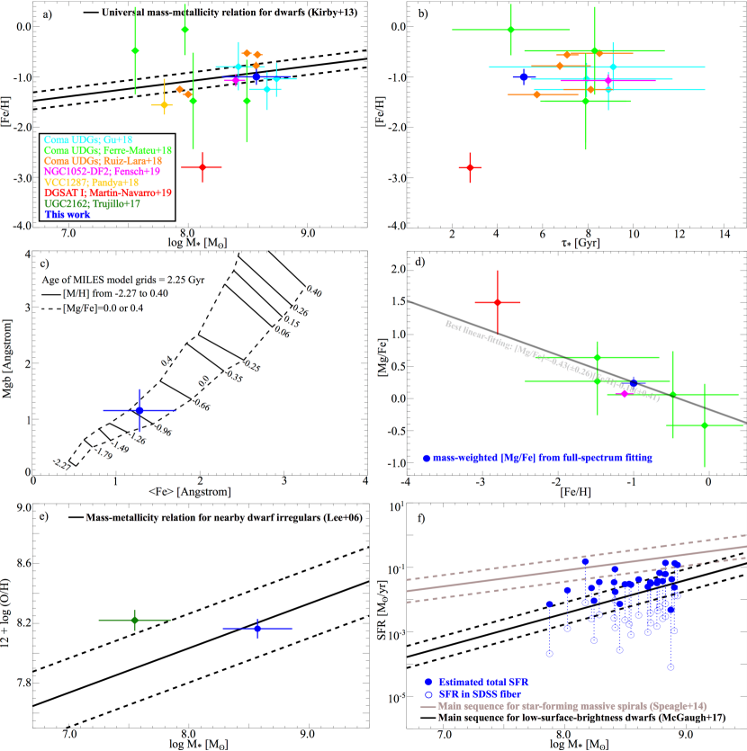
Figure 4: Panel a: stellar metallicities [Fe/H] versus stellar masses $M_{*}$ for UDGs, compared with the universal [Fe/H]-$M_{*}$ relation of nearby dwarf galaxies obtained from Kirby et al. (2013). Panel b: [Fe/H] versus stellar ages $\tau_{*}$ for UDGs. Panel c: Mgb vs. $\langle{\rm{Fe}}\rangle$ of our UDGs plotted onto the MILES model grids (the model age closest to the light-weighted $t_{*}\sim 2.2$ Gyr, i.e., 2.25 Gyr, is chosen). Panel d: [Mg/Fe] vs. [Fe/H] for UDGs (for our star-forming UDGs, we use the mass-weighted [Mg/Fe] value from the pPXF full-spectrum fitting); the best linear-fitting result for the [Mg/Fe]-[Fe/H] relation of these UDGs is also shown. Panel e: oxygen abundance 12+$\log$(O/H) as a function of $M_{*}$ for UDGs, compared with the mass-metallicity relation for nearby star-forming dwarfs obtained by Lee et al. (2006). Panel f: SFRs vs. $M_{*}$ for UDGs, compared with the main sequences of star-forming massive spirals (brown) and low-surface-brightness dwarfs (black) obtained by Speagle et al. (2014) and McGaugh et al. (2017), respectively; the blue closed circles and open circles show the estimated total SFRs (i.e., upper-limits) and SFRs covered by the SDSS 3 arcsec fiber (the two SFRs of each UDG is linked by a dotted line), respectively. In the six panels, the blue color always denotes our UDGs in this work, while the cyan, light-green, orange, magenta, yellow, red, and dark-green diamonds denote the UDGs in previous literature of Gu et al. (2018), Ferré-Mateu et al. (2018), Ruiz-Lara et al. (2018), Fensch et al. (2019), Pandya et al. (2018), Martín-Navarro et al. (2019), and Trujillo et al. (2017), respectively (indicated in the inset of panel a).

To estimate the on-average stellar velocity dispersion $\sigma_{\rm{los}}$ of our UDGs, we set the additive polynomials of the 12th order and multiplicative polynomials of the 14th order (Fensch et al., 2019), and fit the stacked spectrum again. We find $\sigma_{\rm{los}}\simeq 54\pm 12$ km/s for our UDGs, comparable to the high dispersion of DGSAT I (Martín-Navarro et al., 2019). However, note that $\sigma_{\rm{los}}$ only suggests the central stellar dispersion of our UDGs, since the SDSS fiber primarily targets at the central regions of our UDGs.

Gas-phase properties: After subtracting the best-fit stellar models from the stacked spectrum, we then use a Gaussian profile to fit each emission line carefully and estimate the on-average gas-phase metallicity. Since the [O ii] lines are not covered by the wavelength range of the stacked spectrum, we use two additional powerful diagnostics, i.e., N2S2H$\alpha$ defined by Dopita et al. (2016) and O3N2 described in Pettini & Pagel (2004), to estimate the oxygen abundance, respectively. The former diagnostic makes use of the flux ratios of [N ii]$\lambda 6584$/H$\alpha$ and [N ii]$\lambda 6584$/[S ii]$\lambda\lambda$6717,31, while the latter one applies [O iii]$\lambda 5007$/H$\beta$ and [N ii]$\lambda 6584$/H$\alpha$, to determine the O/H ratio. By the uses of emission lines located close together in wavelength, the two diagnostics are actually independent of the internal extinction. We obtain 12+$\log$(O/H)$\simeq 7.94\pm 0.10$ (N2S2H$\alpha$) and $\simeq 8.38\pm 0.07$ (O3N2) for our UDGs, and treat the mean 12+$\log$(O/H) value from the two diagnostics as the final on-average metallicity. As shown in panel e of Fig. 4, we find that, different from the relatively-high oxygen abundance of the star-forming UDG UGC 2162 ($g-r\simeq 0.45$, 12+$\log$(O/H)=$8.22\pm 0.07$; Trujillo et al., 2017), the on-average oxygen abundance of our UDGs follow (within $1\sigma$ uncertainty) the 12+$\log$(O/H)-$M_{*}$ relation of the nearby star-forming dwarf galaxies (Lee et al., 2006), confirming again that our UDGs in the low-density environments are not particularly metal-poor or metal-rich.

In order to assess the star-formation rate (SFR) of each UDG, we impose to fit the spectrum of each UDG with the optimal stellar template, and derive the H$\alpha$ emission line flux covered by the SDSS $3^{\prime\prime}$ fiber from the residual spectrum. The SFR in fiber aperture, SFR_fiber, is obtained by adopting the H$\alpha$ luminosity-SFR relation of Kennicutt (1994). We also estimate the total SFR of each UDG by using the ratio of luminosities of the region covered by the fiber and entire galaxy; note that the total SFR is actually the upper-limit, since the SDSS fiber primarily targets at the central regions of our UDGs, while the star formation in a dwarf galaxy is usually concentrated at the central region. As shown in panel f of Fig. 4, on the SFR versus $M_{*}$ diagram, our UDGs are distributed lower than the extrapolated star-forming main sequence from the massive spirals (brown; Speagle et al., 2014), but plausibly follow (or be slightly lower than) the main sequence of the low-surface-brightness dwarf galaxies (black; McGaugh et al., 2017), suggesting a possible lower star-formation efficiency (i.e., low SFR/H₂) or HI-to-H₂ ratio in these UDGs.

4 Discussion

In this work, for our small UDG sample including 28 members, we used the bootstrap methodology to estimate the uncertainty of each on-average property. We randomly sampled the spectra of the 28 UDGs with replacement for 1,000 times; in each sampling, we stack the 28 sampled spectra and fit the stacked spectrum following the steps described in section 3, and thus obtain 1,000 numbers of $t_{*}$, [M/H], [$\alpha$/Fe], line indices, emission-line fluxes, and dispersions, etc. For $t_{*}$, [M/H], line indices, and emission-line fluxes, their standard deviations $\sigma_{\rm{std}}$ are treated as the uncertainties. For [$\alpha$/Fe], since we linearly interpolated the SSP models between [$\alpha$/Fe]=0 and 0.4 dex with a spacing of 0.1 dex, we included an additional error of $\sim 0.1$ dex which is the maximum [$\alpha$/Fe] uncertainty possibly introduced by interpolation, i.e., the [$\alpha$/Fe] uncertainty $\simeq\sqrt{\sigma_{\rm{std}}^{2}+0.1^{2}}$. For $\sigma_{\rm{los}}$, we included the average redshift uncertainty of the 28 UDGs, i.e., $\sigma_{z}\sim 2.4\times 10^{-5}$ corresponding to a dispersion error of $\sim 7$ km/s, therefore, the stellar dispersion uncertainty $\simeq\sqrt{\sigma_{\rm{std}}^{2}+7^{2}}$.

Since our UDGs have very-extended SFH and assembled their 50% and 90% stellar masses at $z\sim 1.2$ and $\sim 0.2$ respectively, it may reject the current failed $L^{*}$ UDG formation model (Yozin & Bekki, 2015), where UDGs should be quenched at $z\gtrsim 2$. Besides, the tidal interaction with massive galaxies is also very unlikely to be the formation mechanism for our relatively-isolated UDGs.

The light-weighted stellar age ($t_{*}\sim 2.2\pm 0.7$ Gyr) from the pPXF full-spectrum fitting is smaller than the mass-weighted age ($t_{*}\sim 5.2\pm 0.5$ Gyr); as shown in panel d of Fig. 3, 30% light is contributed by the recently-formed stars with $t_{*}<1$ Gyr. These suggest that the light-weighted metallicity values should be significantly affected by the youngest stars. However, the light-weighted metallicities (including [M/H] and [$\alpha$/Fe]) are comparable to the mass-weighted metallicities; it probably indicates that the metal-rich outflows or metal-poor inflows reduced the metallicities produced by the previous generations of stellar populations, since the recently-formed stars in our UDGs do not show significantly-higher metallicities than the underlying old stellar populations. The results may be compatible with the current stellar-feedback model of Chan et al. (2018) or high-spin model of Rong et al. (2017a), which can predict the outflows or inflows during the formation of isolated UDGs as well as present-day star-forming UDGs with the low specific SFRs and stellar ages/metallicities similar to our results.

However, it is also worth to note that, our isolated UDGs are not particularly metal-poor/rich for their stellar masses, as their [Fe/H]-$M_{*}$ and 12+$\log$(O/H)-$M_{*}$ relations follow the mass-metallicity relations of typical dwarfs; it suggests that the feedback-driven outflows in UDGs were not particularly stronger than those in the typical dwarf counterparts (e.g., Spitoni et al., 2010).

Yet, note also that our UDGs are relatively-isolated, star-forming, and thus represent the relatively-bright side of UDG populations as shown in Fig. 2; therefore, there may be a systematic property bias of our star-forming UDGs from that of the entire UDG population.

Finally, for panel d of Fig. 4, we indicate that the [Mg/Fe] based on the different SSP models may be different, particularly for the low-metallicity cases; therefore, in order to obtain a more accurate [Mg/Fe] vs. [Fe/H] relation, the [Mg/Fe] of NGC 1052-DF2 obtained from the SSP models of Thomas et al. (2011) (TMJ11) should be estimated again with the MILES SSP models (Fensch et al., 2019). Using the line indices values of NGC 1052-DF2 given by Fensch et al. (2019), we find that TMJ11 gives a lower [Mg/Fe], compared with the MILES models (with a difference of $\Delta$[Mg/Fe]$\sim 0.3$ dex). After the revision, we obtain a corrected relation of [Mg/Fe]$\simeq-0.43(\pm 0.26)$[Fe/H]$-0.14(\pm 0.40)$ for UDGs.

References

- Bennett et al. (2014) Bennett, C. L., Larson, D., Weiland, J. L., Hinshaw, G. 2014, ApJ, 794, 135
- Boecker et al. (2020) Boecker, A., Leaman, R., van de Ven, G., Norris, M. A., Mackereth, T., Crain, R. A. 2020, MNRAS, 491, 823
- Cappellari (2017) Cappellari, M. 2017, MNRAS, 466, 798
- Chan et al. (2018) Chan, T. K., Keres, D., Wetzel, A., Hopkins, P. F., Faucher-Giguère, C. -A., El-Badry, K., Garrison-Kimmel, S., Boylan-Kolchin, M. MNRAS, 2018, 478, 906
- Christensen et al. (2018) Christensen, C. R., Davé, R., Brooks, A., Quinn, T., Shen, S. 2018, ApJ, 867, 142
- Dopita et al. (2016) Dopita, M. A., Kewley, L. J., Sutherland, R. S., Nicholls, D. C. 2016, Astrophysics and Space Science, 361, 61
- Eigenthaler et al. (2018) Eigenthaler, P., et al. 2018, ApJ, 855, 142
- Fahrion et al. (2019) Fahrion, K., et al. 2019, A&A, 628, 92
- Fensch et al. (2019) Fensch, J., et al. 2019, A&A, 625, 77
- Ferrarese et al. (2012) Ferrarese, L., et al. 2012, ApJS, 200, 4
- Ferré-Mateu et al. (2018) Ferré-Mateu, A., et al. 2018, MNRAS, 479, 4891
- Fitzpatrick (1999) Fitzpatrick, E. L. 1999, PASP, 111, 63
- Guo et al. (2020) Guo, Q., et al., 2020, Nature Astronomy, 4, 246
- Gu et al. (2018) Gu, M., et al. 2018, ApJ, 859, 37
- Guérou et al. (2017) Guérou, A., et al. 2017, A&A, 608, 5
- Ho et al. (2011) Ho, L. C., Li, Z.-Y., Barth, A. J., Seigar, M. S., Peng, C. Y. 2011, ApJS, 197, 21
- Kennicutt (1994) Kennicutt, R. C., Tamblyn, P., Congdon, C.W. 1994, ApJ, 435, 22
- Kirby et al. (2013) Kirby, E. N., Cohen, J. G., Guhathakurta, P., Cheng, L., Bullock, J. S., Gallazzi, A. 2013, ApJ, 779, 102
- Lee et al. (2006) Lee, H., Skillman, E. D., Cannon, J. M., et al. 2006, ApJ, 647, 970
- Leisman et al. (2017) Leisman, L., et al. 2017, ApJ, 842, 133
- Martín-Navarro et al. (2019) Martín-Navarro, I., et al. 2019, MNRAS, 484, 3425
- McDermid et al. (2015) McDermid, R. M., et al. 2015, MNRAS, 448, 3484
- McGaugh et al. (2017) McGaugh, S. S., Schombert, J. M., Lelli, F. 2017, ApJ, 851, 22
- Mihos et al. (2015) Mihos, J. C., et al. 2015, ApJ, 809L, 21
- Pandya et al. (2018) Pandya, V., et al. 2018, ApJ, 858, 29
- Peng et al. (2010) Peng, C. Y., Ho, L. C., Impey, C. D., Rix, H.-W. 2010, AJ, 139, 2097
- Pettini & Pagel (2004) Pettini, M. & Pagel, B. E. J. 2004, MNRAS, 348, L59
- Pietrinferni et al. (2006) Pietrinferni, A., Cassisi, S., Salaris, M., Castelli, F. 2006, ApJ, 642, 797
- Rong et al. (2017a) Rong, Y., Guo, Q., Gao, L., Liao, S., Xie, L., Puzia, T. H., Sun, S., Pan, J. 2017a, MNRAS, 470, 4231
- Rong et al. (2018) Rong, Y., Li, H., Wang, J., et al. 2018, MNRAS, 477, 230
- Rong et al. (2017b) Rong, Y., Jing, Y., Gao, L., Guo, Q., Wang, J., Sun, S., Wang, L., Pan, J. 2017b, MNRAS, 471L, 36
- Rong et al. (2019a) Rong, Y., et al., 2019a, ApJ, 883, 56
- Rong et al. (2019b) Rong, Y., et al., 2019b, eprint arXiv: 1907.10079
- Rong et al. (2020) Rong, Y., Mancera Piña, P. E., Tempel, E., Puzia, T. H., De Rijcke, S. 2020, eprint arXiv: 2007.06593
- Rupke et al. (2010) Rupke, D. S. N., Kewley, L. J., Barnes, J. E. 2010, ApJ, 710L, 156
- Ruiz-Lara et al. (2018) Ruiz-Lara, T., et al. 2018, MNRAS, 478, 2034
- Saulder et al. (2016) Saulder, C., van Kampen, E., Chilingarian, I. V., Mieske, S., Zeilinger, W. W. 2016, A&A, 596, 14
- Simard et al. (2011) Simard, L., Mendel, J. T., Patton, D. R., Ellison, S. L., McConnachie, A. W. 2011, ApJS, 196, 11
- Speagle et al. (2014) Speagle, J. S., Steinhardt, C. L., Capak, P. L., Silverman, J. D. 2014, ApJS, 214, 15
- Spitoni et al. (2010) Spitoni,E., Calura, F., Matteucci, F., Recchi, S. 2010, A&A, 514, 73
- Thomas et al. (2005) Thomas, D., Maraston, C., Bender, R., Mendes de Oliveira, C. 2005, ApJ, 621, 673
- Thomas et al. (2011) Thomas, D., Maraston, C., Johansson, J. 2011, MNRAS, 412, 2183
- Trujillo et al. (2017) Trujillo, I., Roman, J., Filho, M., Sánchez Almeida, J. 2017, ApJ, 836, 191
- van Dokkum et al. (2015) van Dokkum, P. G., Abraham, R., Merritt, A., Zhang, J., Geha, M., Conroy, C. 2015, ApJ, 798L, 45
- van Dokkum et al. (2016) van Dokkum, P. G., et al. 2016, ApJL, 828, 6
- van Dokkum et al. (2018) van Dokkum, P. G., et al. 2018, Nature, 555, 629
- Vazdekis et al. (2015) Vazdekis, A., et al. 2015, MNRAS, 449, 1177
- Worthey et al. (1994) Worthey, G., Faber, S. M. Gonzalez, J. J., Burstein, D. 1994, ApJS, 94, 687
- Yagi et al. (2016) Yagi, M., Koda, J., Komiyama, Y., Yamanoi, H. 2016, ApJS, 225, 11
- Yozin & Bekki (2015) Yozin, C., Bekki, K. 2015, MNRAS, 452, 937