Generalized likelihood ratio test detector
for a modified replacement model target
in a multivariate $t$-distributed background

Abstract

A closed-form expression is derived for the generalized likelihood ratio test (GLRT) detector of a subpixel target in a multispectral image whose area and brightness are both unknown. This expression extends a previous result (which assumed a Gaussian background distribution) to a fatter tailed elliptically-contoured (EC) multivariate $t$-distributed background. Numerical experiments with simulated data indicate that the EC-based detector outperforms the simpler Gaussian-based detectors, and that the relative performance of the new detector, compared to other EC-based detectors depends on the regime of target strength and background occlusion.

I Introduction

To obtain a signal processing solution to the problem of subpixel target detection in hyperspectral imagery, one requires a model for the target signature, a model for the background distribution, and a model for how the target signal interacts with the background.

Usually the target signature is treated as “known.” Although this signature can exhibit considerable variability due to both extrinsic environmental factors and intrinsic material factors[1], the extent of this variability is in most cases assumed to be known, and is very often treated as a constant.

The background is not “known” in the same a priori sense that the target is known, but it is modeled by a probability distribution that can often be estimated directly from the hyperspectral imagery in which the target is sought. The Gaussian is perhaps the most popular choice; it is parameterized by a mean vector $\mu$ and covariance matrix $R$. The multivariate $t$ distribution is an attractive choice: like the Gaussian, it requires a vector-valued mean and a matrix-valued covariance, but it takes one further parameter, the scalar $\nu$, which characterizes the tail of the distribution. The multivariate $t$ is an elliptically contoured (EC) distribution, because the contours of constant probability density are ellipsoids centered at $\mu$ (indeed, the same ellipsoids that characterize contours of the Gaussian distribution), but it exhibits fatter tails than a Gaussian. Manolakis et al.[2, 3] have argued that these fatter-tailed EC distributions are appropriate for modeling hyperspectral background variability.

Several models have been described that characterize how the target interacts with the background. For an opaque target that occupies a full pixel, there is no interaction, and the detector is straightforward to the point of trivial. Here, we have a simple hypothesis testing problem:

$$H_{o} :\mathbf{x}=\mathbf{z}$$ (1)

$$H_{1} :\mathbf{x}=\mathbf{t}$$ (2)

where $\mathbf{x}$ is the observed spectrum at a pixel, $\mathbf{z}$ is the background at that pixel (i.e., what the spectrum would be if no target were present), and $\mathbf{t}$ is the target spectrum. There are no nuisance parameters in this model, so the optimal detector is given by the likelihood ratio $\mathcal{D}(\mathbf{x})=p_{t}(\mathbf{x})/p_{z}(\mathbf{x})$, where $p_{z}$ and $p_{t}$ are the probability density functions associated with the background and target, respectively. We can interpret $p_{z}(\mathbf{x})$ is the likelihood of observing $\mathbf{x}$ in a background pixel, and $p_{t}(\mathbf{x})$ as the likelihood of observing $\mathbf{x}$ in a target pixel.

For subpixel targets (or for models that incorporate adjacency effects, or include translucency, such as gas-phase plume targets[4]), there is an interaction of target with background. The most common models are the additive and replacement models, though Vincent and Besson[5] have recently suggested a hybrid “modified replacement” model that generalizes both of them, though at the cost of introducing a second parameter:

$H_{1}$:	$\mathbf{x}=\mathbf{z}+\alpha\mathbf{t}$	Additive model
$H_{1}$:	$\mathbf{x}=(1-\alpha)\mathbf{z}+\alpha\mathbf{t}$	Replacement model
$H_{1}$:	$\mathbf{x}=\beta\mathbf{z}+\alpha\mathbf{t}$	Modified replacement model

The additive model corresponds to a target whose strength depends on $\alpha$, where “strength” in this case might correspond to intrinsic brightness (or reflectance) of the target, depending on linear factors that might include illumination, temperature (for infrared imaging), concentration (especially for gas-phase plumes), etc. The replacement model treats the subpixel target as opaque, and having an area (relative to the pixel size) of $\alpha$; thus its contribution to the observed signal is proportional to $\alpha$ but the contribution of the background is correspondingly diminished by a factor of $1-\alpha$. The modified replacement model is attractive in that it can account both for the diminishing background contribution ($\beta<1$) due to an opaque (or partially opaque) target, and for target strength variability due to more intrinsic brightness effects. Solid materials often exhibit spectral variability due, for instance, to powder grain size, and although that variability may be somewhat complex, it is often seen in practice that the dominant effect is in the overall magnitude of the reflectance of the material.

Unlike the full-pixel case, the alternative hypotheses (the $H_{1}$’s) for these target-background interaction models involve unknown, or nuisance, parameters: $\alpha$, or $\alpha$ and $\beta$. For this reason, they are not simple but composite hypothesis testing problems. There are a number of approaches for dealing with composite hypothesis testing problems: Bayes factor[6], penalized likelihood[7, 8], and clairvoyant fusion[9, 10] among them. The most popular, and usually quite effective (albeit not always optimal[11]), is the generalized likelihood ratio test (GLRT), which is based on maximizing the likelihoods used in the likelihood ratio test, or equivalently on employing maximum likelihood estimates of the nuisance parameters in the likelihood ratio test.

Using the GLRT, closed-form expressions have been identified for a variety of target models on a variety of background distributions.

For an additive target on a Gaussian background, the adaptive matched filter (AMF) is the appropriate detector[12, 13]; indeed, it is provably optimal as the uniformly most powerful (UMP) detector[6]. For solid subpixel targets, a replacement model is appropriate. The target signal is proportional to the fraction $a$ of the pixel that the target covers, but the background is occluded by that same fraction. For Gaussian background, this leads to the finite target matched filter (FTMF)[14]. Finally, a generalization of additive and replacement is given by the modified replacement model: here both the target and the background scale, and the Gaussian GLRT is given by Vincent and Bresson[5]. In [5], both one-step and two-step variants are derived, and the one-step variant is called SPADE (Sub-Pixel Adaptive DEtection); the interest in this paper is with the two-step variant, which I will call 2SPADE.

These are two-step detectors; the mean and covariance are computed from a (large) sample of off-target pixels, and are treated as exact and fixed for the pixels under test. For global methods (in which a single mean and covariance is estimated for the whole image) and even for semi-local methods (in which the mean is computed locally, but a single global covariance is estimated), the sample size will be large and the two-step methods are appropriate. In practice, we may not know if a set of pixels are truly target-free, and in that case some level of contamination may occur. As long as the contaminating targets are rare and/or weak, the effect of this contamination will usually be small[15].

But for local methods, in which both the mean and covariance are recomputed in a (small) moving window, the one-step methods are potentially better detectors because they account for the statistical imprecision in the estimates of mean and covariance. The one-step derivations are more difficult to derive, but a one-step AMF is given by Kelly[16], and one-step replacement (ACUTE) by Vincent and Bresson[17], and one-step modified replacement (SPADE)[5]. In all three of these cases, as the sample size becomes large, the one-step detector approaches the two-step detector.

The extension of these two-step detectors to elliptically-contoured multivariate $t$-distributed backgrounds has been developed for the additive[18] and for the replacement[19] models. In this exposition, the two-step modified replacement model will be extended to an elliptically contoured background, here called EC-2SPADE.

Also, beyond Gaussian and multivariate-$t$ are non-parametric methods, such as NP-AMF[20], which enable far more flexible modeling of the background.

TABLE I: Summary of detectors for various target models on various background distributions. The EC-2SPADE detector is derived in this paper.

Target Model		Background distribution
Model Name	Expression	Gaussian	multivariate $t$
Additive	$\mathbf{x}=\mathbf{z}+\alpha\mathbf{t}$	AMF[12, 13]	EC-AMF[18]
Replacement	$\mathbf{x}=(1-\alpha)\mathbf{z}+\alpha\mathbf{t}$	FTMF[14]	EC-FTMF[19]
Modified	$\mathbf{x}=\beta\mathbf{z}+\alpha\mathbf{t}$	2SPADE[5]	EC-2SPADE

II Set up the problem

II-A Background model

In the absence of target, the background is assumed to be distributed as a multivariate $t$ distribution. A background pixel spectrum is denoted $\mathbf{z}\in\mathbb{R}^{d}$ where $d$ is the number of spectral channels in the hyperspectral imagery. Here,

$$p_{z}(\mathbf{z})=c\left[(\nu-2)+\mathcal{A}(\mathbf{z})\right]^{-(d+\nu)/2}$$ (3)

where $c$ is a normalizing constant, $\nu$ is a scalar parameter that characterizes the tail of the distribution, and

$$\mathcal{A}(\mathbf{z})=(\mathbf{z}-\mbox{\boldmath{$\mu$}})^{\prime}R^{-1}(\mathbf{z}-\mbox{\boldmath{$\mu$}})$$ (4)

is a squared Mahalanobis distance. Here, $\mu$ and $R$ are the mean and covariance of the background, and the fact that $p(\mathbf{z})$ depends on $\mathbf{z}$ through $\mathcal{A}(\mathbf{z})$ ensures that the distribution is elliptically contoured. Note that in the limit as $\nu\to\infty$, the distribution becomes Gaussian. For $\nu\leq 2$, the distribution is so fat-tailed that the second moment does not exist.

II-B Target-background interaction model

Under the null hypothesis (which is that the target is not present in the given pixel), the observed spectrum is the background. The alternative hypothesis is that the target is present. The target has a known signature $\mathbf{t}$, but what is observed is a linear combination of target and background. Thus:

$$H_{o} :\mathbf{x}=\mathbf{z}$$ (5)

$$H_{1} :\mathbf{x}=\beta\mathbf{z}+\alpha\mathbf{t}$$ (6)

with constraints $0\leq\beta\leq 1$ and $0\leq\alpha$.

III GLRT solution

Because this is a two-step solution, we will begin with the assumption that we have an adequate estimate of $\mu$, $R$, and $\nu$, usually obtained from a large number of background pixels.

Under the hypothesis that a target is present, we have $\mathbf{x}=\beta\mathbf{z}+\alpha\mathbf{t}$, where $\beta$ and $\alpha$ are unknown. Then

$$\mathbf{z}=\frac{\mathbf{x}-\alpha\mathbf{t}}{\beta}$$ (7)

and the probability distribution associated with observation $\mathbf{x}$ is given by

$$p_{x}(\alpha,\beta;\,\mathbf{x}) =p_{z}(\mathbf{z})\left|\frac{d\mathbf{z}}{d\mathbf{x}}\right|=p_{z}\left(\frac{\mathbf{x}-\alpha\mathbf{t}}{\beta}\right)\cdot\beta^{-d}$$ (8)

$$=c\beta^{-d}\left[(\nu-2)+\mathcal{A}\left(\frac{\mathbf{x}-\alpha\mathbf{t}}{\beta}\right)\right]^{-(d+\nu)/2}$$ (9)

The GLRT detector the is based on the likelihood ratio, maximized over the nuisance parameters; specifically

$$\mathcal{D}(\mathbf{x})=\frac{\max_{\alpha,\beta}p_{x}(\alpha,\beta;\,\mathbf{x})}{p_{x}(0,1;\mathbf{x})}=\frac{p_{x}(\widehat{\alpha},\widehat{\beta};\,\mathbf{x})}{p_{z}(\mathbf{x})}$$ (10)

where $\widehat{\alpha}$ and $\widehat{\beta}$ are the values (they are both functions of $\mathbf{x}$) that maximize $p_{x}(\alpha,\beta;\,\mathbf{x})$.

We will begin with maximization over $\alpha$. This occurs at

$$\widehat{\alpha} =\mbox{argmax}_{\alpha}~{}p_{x}(\alpha,\beta;\,\mathbf{x})$$ (11)

$$=\mbox{argmax}_{\alpha}~{}\mathcal{A}\left(\frac{\mathbf{x}-\alpha\mathbf{t}}{\beta}\right)$$ (12)

$$=\mbox{argmax}_{\alpha}~{}(\mathbf{x}-\alpha\mathbf{t}-\beta\mbox{\boldmath{$\mu$}})^{\prime}R^{-1}(\mathbf{x}-\alpha\mathbf{t}-\beta\mbox{\boldmath{$\mu$}})$$ (13)

$$=\frac{\mathbf{t}^{\prime}R^{-1}(\mathbf{x}-\beta\mbox{\boldmath{$\mu$}})}{\mathbf{t}^{\prime}R^{-1}\mathbf{t}}$$ (14)

Observe that

$$\frac{\mathbf{x}-\widehat{\alpha}\mathbf{t}}{\beta}-\mbox{\boldmath{$\mu$}}=\frac{1}{\beta}\left(I-\frac{\mathbf{t}\mathbf{t}^{\prime}R^{-1}}{\mathbf{t}^{\prime}R^{-1}\mathbf{t}}\right)(\mathbf{x}-\beta\mbox{\boldmath{$\mu$}})$$ (15)

Thus, if we write

$$Q=\left(I-\frac{\mathbf{t}\mathbf{t}^{\prime}R^{-1}}{\mathbf{t}^{\prime}R^{-1}\mathbf{t}}\right)^{\prime}R^{-1}\left(I-\frac{\mathbf{t}\mathbf{t}^{\prime}R^{-1}}{\mathbf{t}^{\prime}R^{-1}\mathbf{t}}\right)$$ (16)

then we have

$$\mathcal{A}\left(\frac{\mathbf{x}-\widehat{\alpha}\mathbf{t}}{\beta}\right) =\frac{(\mathbf{x}-\beta\mbox{\boldmath{$\mu$}})^{\prime}Q(\mathbf{x}-\beta\mbox{\boldmath{$\mu$}})}{\beta^{2}}$$ (17)

$$=a+b\beta^{-1}+c\beta^{-2}=q(\beta)$$ (18)

where $q(\beta)$ is a scalar quadratic expression in $\beta^{-1}$ with

$$a =\mbox{\boldmath{$\mu$}}^{\prime}Q\mbox{\boldmath{$\mu$}},$$ (19)

$$b =-2\mbox{\boldmath{$\mu$}}^{\prime}Q\mathbf{x},$$ (20)

$$c =\mathbf{x}^{\prime}Q\mathbf{x}.$$ (21)

With $\alpha=\widehat{\alpha}$, our expression for likelihood in Eq. (9) becomes

$$p_{x}(\beta;\,\mathbf{x}) =p_{x}(\widehat{\alpha}(\beta,\mathbf{x}),\beta;\,\mathbf{x})$$ (22)

$$=c\beta^{-d}\left[(\nu-2)+q(\beta)\right]^{-(d+\nu)/2}$$ (23)

Writing the log likelihood (minus a constant) for hypothesis $H_{1}$, we have

$$L_{1}(\beta;\,\mathbf{x}) =\log p_{x}(\beta;\,\mathbf{x})-\log c$$ (24)

$$=-d\log\beta-\frac{d+\nu}{2}\log\left[(\nu-2)+q(\beta)\right]$$ (25)

To maximize this log likelihood we take the derivative with respect to $\beta$ and set the result to zero:

$$0=\frac{\partial}{\partial\beta}L_{1}(\beta;\,\mathbf{x})=-d\beta^{-1}-\frac{d+\nu}{2}\frac{\frac{\partial}{\partial\beta}q(\beta)}{(\nu-2)+q(\beta)}$$ (26)

Multiplying both sides by $(\nu-2)+q(\beta)$, we obtain

$$0 =-d\beta^{-1}[(\nu-2)+q(\beta)]-\frac{d+\nu}{2}[-b\beta^{-2}-2c\beta^{-3}]$$ (27)

Now, multiply both sides by $-\beta^{3}/\nu$:

$$0 =\frac{d(\nu-2+a)}{\nu}\beta^{2}+\frac{db}{\nu}\beta+dc+\frac{d+\nu}{2\nu}[-b\beta-2c]$$ (28)

$$=A\beta^{2}+B\beta+C$$ (29)

which is a quadratic equation in $\beta$ and can be solved in closed-form. Here,

$$A =d+\frac{d(a-2)}{\nu}$$ (30)

$$B =-\frac{b}{2}+\frac{db}{2\nu}$$ (31)

$$C =-c$$ (32)

from which

$$\widehat{\beta}=\mbox{min}\left(\frac{-B+\sqrt{B^{2}-4AC}}{2A},1\right)$$ (33)

Note that since $A>0$ and $C<0$, we can be sure that $\widehat{\beta}>0$. We can further observe that $\widehat{\beta}=1$ whenever $-C\geq(A+B)$.

Finally, given $\widehat{\alpha}$ from Eq. (14) and $\widehat{\beta}$ from Eq. (33), the GLRT target detector for the modified replacement model is given by Eq. (10).

III-A Special case: $\nu\to\infty$

In the $\nu\to\infty$ limit, the EC distribution becomes Gaussian. The expressions for $A$, $B$, and $C$ become

$$A =d$$ (34)

$$B =-b/2=\mbox{\boldmath{$\mu$}}^{\prime}Q\mathbf{x}$$ (35)

$$C =-c=-\mathbf{x}^{\prime}Q\mathbf{x}$$ (36)

which is consistent with Eq(6) from Ref. [5].

III-B Remark on $Q$

Note that Eq. (16) can equivalently be written

$$Q=R^{-1/2}\left(I-\frac{R^{-1/2}\mathbf{t}\mathbf{t}^{\prime}R^{-1/2}}{\mathbf{t}^{\prime}R^{-1}\mathbf{t}}\right)R^{-1/2}$$ (37)

which can be interpreted as a projection operator sandwiched between two whitening operators. If we consider the matched filter vector

$$\mathbf{q}=R^{-1}\mathbf{t}/\sqrt{t^{\prime}R^{-1}\mathbf{t}}$$ (38)

then we have another expression for $Q$ given by

$$Q=R^{-1}-\mathbf{q}\mathbf{q}^{\prime}$$ (39)

IV Clairvoyant detector

If $\alpha$ and $\beta$ were known, then the so-called clairvoyant detector[21] provides optimal detection, but it is an odd scenario to know the strength of the target without knowing whether or not the target is present. Still, the clairvoyant provides a useful upper bound on the performance of a target detector, and shows the penalty paid by replacing the true (but unkonwn) $\alpha$ and $\beta$ with the estimates $\widehat{\alpha}$ and $\widehat{\beta}$ which are recomputed for each pixel. The detector is given by any monotonic transform ($h$) of the likelihood ratio:

$$\mathcal{D}(\alpha,\beta,\mathbf{x})=h\left(\frac{p_{x}(\alpha,\beta;\,\mathbf{x})}{p_{z}(\mathbf{x})}\right).$$ (40)

If we let

$$h(w)=\frac{\exp\left(\frac{2}{d+\nu}\left[\log w+d\log\beta\right]\right)-1}{\nu-2},$$ (41)

then

$$\mathcal{D}(\alpha,\beta,\mathbf{x})=\frac{1}{1+\displaystyle\frac{\mathcal{A}(\mathbf{x})}{\nu-2}}\left[\mathcal{A}\left(\frac{\mathbf{x}-\alpha\mathbf{t}}{\beta}\right)-\mathcal{A}(\mathbf{x})\right]$$ (42)

is a clairvoyant detector. In the $\nu\to\infty$ limit, this is simply

$$\mathcal{D}(\alpha,\beta,\mathbf{x})=\mathcal{A}\left(\frac{\mathbf{x}-\alpha\mathbf{t}}{\beta}\right)-\mathcal{A}(\mathbf{x}).$$ (43)

V Numerical illustration

Fig. 1 shows ROC curves, illustrating detector performance for $\alpha=0.2$ and a range of values of $\beta$. One very general trend is that detection becomes harder as $\beta$ gets larger, and more background signal is mixed in with the target signal.

The performance is computed using simulated data, and since that simulated data is based on an elliptically-contoured (EC) multivariate $t$ background, it is not surprising to observe that the EC-based algorithms (shown with solid lines) generally outperform their Gaussian counterparts (dashed lines).

We see for small values of $\beta$ that the 2SPADE and EC-2SPADE are the best detectors, with EC-2SPADE outperforming 2SPADE by a considerable margin. As $\beta$ increases toward $1-\alpha$, the FTMF and EC-FTMF algorithms begin provide the best performance, with EC-FTMF outperforming FTMF. This cross-over in ROC curve performance between 2SPADE and FTMF was also observed by Vincent and Besson[5]. Finally, as $\alpha\to 1$, the EC-AMF exhibits the best performance.

Similar curves are seen in Fig. 2, but here $\alpha=0.6$ which provides more examples with $\alpha+\beta>1$. For $0.3\leq\beta\leq 0.5$, we see that EC-FTMF outperforms EC-2SPADE. For $\beta=0.6$, EC-2SPADE is best, but for $\beta\geq 0.7$, EC-AMF outperforms EC-2SPADE. On the other hand, in none of the cases here is EC-2SPADE the worst detector, and it is never as bad as EC-AMF at small $\beta$ or EC-FTMF at large $\beta$.

Because we are comparing performance to the optimal clairvoyant detector, we can see that, at their points of optimailtiy, the EC-FTMF (at $\beta=1-\alpha=0.8$) and EC-AMF ($\beta=1.0$) detectors are very nearly optimal in their performance. By contrast the EC-2SPADE detector does not seem to approach the performance of the clairvoyant detector. Fitting two parameters instead of one seems to incur a performance penalty.

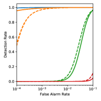
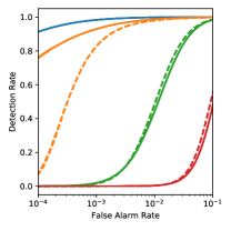
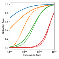
(a) $\beta=0.3$ (b) $\beta=0.4$ (c) $\beta=0.5$ (d) $\beta=0.6$

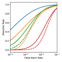
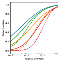
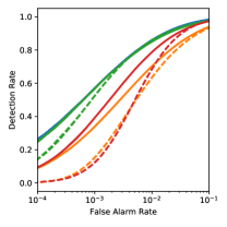
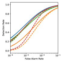
(e) $\beta=0.7$ (f) $\beta=0.8$ (g) $\beta=0.9$ (h) $\beta=1.0$

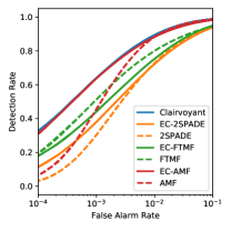
Figure 1: ROC curves showing detector performance for a range of $\beta$ values from 0.3 to 1.0. For these simulations, $N=10^{7}$ matched-pair samples are generated; for each pair, one is without target ($\mathbf{x}=\mathbf{z}$) and one includes target ($\mathbf{x}=\beta\mathbf{z}+\alpha\mathbf{t}$). The data are simulated from a multivariate $t$ distribution, with $d=10$ and $\nu=10$, mean $\mu=[2,2,\ldots,2]^{\prime}$, and unit covariance $R=I$. The target signature is $\mathbf{t}=\mu+[T,0,\ldots,0]$, with $T=15$, and the target strength for all these simulations was $\alpha=0.2$. (Very roughly speaking, the target is “three sigmas” away from the background mean.) Note that three curves are drawn for each case in order to provide a sense of trial-to-trial variability; for the curves here, however, that variability rarely exceeds the linewidth on the plots.

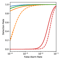
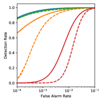
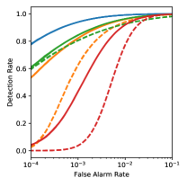
(a) $\beta=0.3$ (b) $\beta=0.4$ (c) $\beta=0.5$ (d) $\beta=0.6$

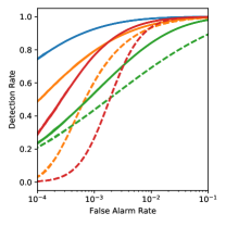
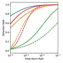
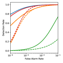
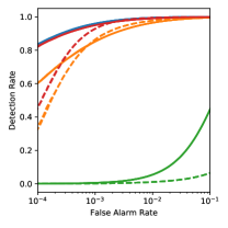
(e) $\beta=0.7$ (f) $\beta=0.8$ (g) $\beta=0.9$ (h) $\beta=1.0$

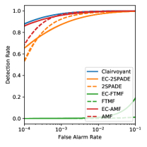
Figure 2: ROC curves showing detector performance for a range of $\beta$ values from 0.3 to 1.0. Same as Fig. 1, but here $\alpha=0.6$ (three times larger) and $T=5$ (three times weaker), so there is still a roughly three-sigma distance from the target to the mean.

VI Discussion

Applied to simulated data, tailored to the assumptions of the new detector, the new detector performs well. Further work will be needed to examine how well this detector behaves in the “wild,” with real targets in real imagery.

Introducing, and optimizing over, more parameters does lead to a more flexible detector, but not necessarily a more powerful one. We saw that imposing an assumption (e.g., that $\beta=1-\alpha$) that reduced the number of free parameters led to improved detection performance even when the assumption was only approximately true.

References

- [1] J. Theiler, A. Ziemann, S. Matteoli, and M. Diani, “Spectral variability of remotely-sensed target materials: causes, models, and strategies for mitigation and robust exploitation,” Geoscience and Remote Sensing Magazine, vol. 7, pp. 8–30, June 2019.
- [2] D. Manolakis, D. Marden, J. Kerekes, and G. Shaw, “On the statistics of hyperspectral imaging data,” Proc. SPIE, vol. 4381, pp. 308–316, 2001.
- [3] D. B. Marden and D. Manolakis, “Using elliptically contoured distributions to model hyperspectral imaging data and generate statistically similar synthetic data,” Proc. SPIE, vol. 5425, pp. 558–572, 2004.
- [4] J. Theiler and A. Schaum, “Some closed-form expressions for absorptive plume detection,” Proc. IEEE International Geoscience and Remote Sensing Symposium (IGARSS), 2020, to appear.
- [5] F. Vincent and O. Besson, “Generalized likelihood ratio test for modified replacement model in hyperspectral imaging detection,” Signal Processing, vol. 174, p. 107643, 2020.
- [6] E. L. Lehmann and J. P. Romano, Testing Statistical Hypotheses. New York: Springer, 2005.
- [7] J. Chen, “Penalized likelihood-ratio test for finite mixture models with multinomial observations,” Canadian Journal of Statistics, vol. 26, pp. 583–599, 1998.
- [8] A. Vexler, C. Wu, and K. F. Yu, “Optimal hypothesis testing: from semi to fully Bayes factors,” Metrika, vol. 71, pp. 125–138, 2010.
- [9] A. Schaum, “Continuum fusion: a theory of inference, with applications to hyperspectral detection,” Optics Express, vol. 18, pp. 8171–8181, 2010.
- [10] ——, “Clairvoyant fusion: a new methodology for designing robust detection algorithms,” Proc. SPIE, vol. 10004, p. 100040C, 2016.
- [11] J. Theiler, “Confusion and clairvoyance: some remarks on the composite hypothesis testing problem,” Proc. SPIE, vol. 8390, p. 839003, 2012.
- [12] I. S. Reed, J. D. Mallett, and L. E. Brennan, “Rapid convergence rate in adaptive arrays,” IEEE Trans. Aerospace and Electronic Systems, vol. 10, pp. 853–863, 1974.
- [13] F. C. Robey, D. R. Fuhrmann, E. J. Kelly, and R. Nitzberg, “A CFAR adaptive matched filter detector,” IEEE Trans. Aerospace and Electronic Systems, vol. 28, pp. 208–216, 1992.
- [14] A. Schaum and A. Stocker, “Spectrally selective target detection,” in Proc. ISSSR (Int. Symp. Spectral Sensing Research), 1997, p. 23.
- [15] J. Theiler and B. R. Foy, “Effect of signal contamination in matched-filter detection of the signal on a cluttered background,” IEEE Geoscience and Remote Sensing Letters, vol. 3, pp. 98–102, 2006.
- [16] E. J. Kelly, “Performance of an adaptive detection algorithm: rejection of unwanted signals,” IEEE Trans. Aerospace and Electronic Systems, vol. 25, pp. 122–133, 1989.
- [17] F. Vincent and O. Besson, “One-step generalized likelihood ratio test for subpixel target detection in hyperspectral imaging,” IEEE Trans. Geoscience and Remote Sensing, pp. 4479–4489, 2020.
- [18] J. Theiler and B. R. Foy, “EC-GLRT: Detecting weak plumes in non-Gaussian hyperspectral clutter using an elliptically-contoured generalized likelihood ratio test,” in Proc. IEEE International Geoscience and Remote Sensing Symposium (IGARSS), 2008, p. I:221.
- [19] J. Theiler, B. Zimmer, and A. Ziemann, “Closed-form detector for solid sub-pixel targets in multivariate t-distributed background clutter,” in Proc. IEEE International Geoscience and Remote Sensing Symposium (IGARSS), 2018, pp. 2773–2776.
- [20] S. Matteoli, M. Diani, and G. Corsini, “Closed-form nonparametric GLRT detector for subpixel targets in hyperspectral images,” IEEE Trans. Aerospace and Electronic Systems, vol. 56, pp. 1568–1581, 2020.
- [21] S. M. Kay, Fundamentals of Statistical Signal Processing: Detection Theory. New Jersey: Prentice Hall, 1998, vol. II.