Abstract

It is known than the inclusion of spatial curvature can modify the evolution of matter perturbations, and affect the Large Scale Structure (LSS) formation. We quantify the effects of the non-zero space curvature in terms of LSS formation for a cosmological model with a running vacuum energy density and a warm dark matter component. The evolution of density perturbations and the modified shape of its power spectrum are constructed and analyzed.

Keywords:  Large scale structure, running cosmological constant, warm dark matter, matter power spectrum

1 Introduction

The fiducial theory in the modern cosmology is based on general relativity (GR) and the concordance model ($\Lambda$CDM), where the main observables, including the large scale properties of the universe, are explained in terms of the dark energy (DE) and dark matter (DM) components [2, 3].

In $\Lambda$CDM, the global expansion of the Universe caused by this DE is provided by the inclusion of the most natural and simple alternative, which is the cosmological constant (CC), characterized by the equation of state $\omega_{\Lambda}=-1$, or $P_{\Lambda}=-\rho_{\Lambda}$. Independent of the difficult CC problem [4], the presence of this constant is also a consistency requirement from the anthropic [5] and quantum field theory viewpoints [6, 7]. In the phenomenological framework the CC is a very successful concept, regardless of some deviations in the equation of state of the DE from $\omega_{DE}=-1$ can not be ruled out (see e.g. [8, 9, 10]). On the other hand, DM also emerges as a necessary element for explaining the observational evidence about the large scale structure (LSS) formation, baryon acoustic oscillations (BAO) and cosmic microwave background (CMB) anisotropies [11, 12, 13].

However, despite of the mentioned success of $\Lambda$CDM, there are still some discrepancies between different cosmic data sets and measurements, which opens up the door to alternatives theories of gravity or new generalizations and extensions of this standard model (see e.g. [14] for the review). Thus, in order to alleviate these tensions is necessary to look for alternatives descriptions for the gravitational sector or for the cosmic components.

Due to the mentioned theoretical importance and the experimental necessity of the CC, it would makes sense then to explore the possibility that it may be slowly varying, in particular, as consequence of the low-energy quantum corrections. In general, such quantum corrections can be consistently described by the renormalization group running within the semiclassical theory (see e.g. [15]) or in quantum gravity [16, 17]. One can note that the quantum gravitational running at low energies (in the IR) is well-defined but phenomenologically almost irrelevant [17], while the semiclassical running of the density of cosmological constant $\rho_{\Lambda}$ in the IR can be formulated only phenomenologically and characterized by a single free parameter $\nu$ [6, 18]. The models based on such a running were originally developed in [19, 20] (background and cosmic perturbations) and [21, 22], producing many interesting developments (see e.g. [23, 24, 25] and references therein).

On the other hand, describing DM component in terms of particles or fields also represents an open question. Besides the theoretical and experimental difficulties in detecting DM, there is a possibility to assume that DM is warm (WDM) instead of cold (CDM). It is known that the relativistic warmness of DM can change the global dynamic of the universe and provide certain phenomenological advantages [26, 27, 28]. The full standard description of WDM implies the use of the Boltzmann equation. However, the problem can be greatly simplified using the reduced relativistic gas model (RRG) [29, 30]. The main point of the RRG is that it assumes the same kinetic energy for all particles of relativistic gas. Such an artificial ideal relativistic gas model has a very simple equation of state with the unique free parameter $b$, characterizing its warmness. On the other hand, this equation of state closely reproduce similar equation in the Jüttner model [31], based on the relativistic Maxwell distribution. These two features enable one to use RRG, e.g., for the simplified phenomenological description of WDM [32, 33, 34]. The simplicity of RRG is especially welcome in the theories with natural complications, such as the cosmological models with running parameters. As far as most interesting models of running $\rho_{\Lambda}$ (see e.g. [19] and [20]) are consistently applicable only at high energy scale, we need to formulate them in the framework of early universe, when the DM is supposed to have more warmness than today. Then the RRG becomes a useful tool that enables to get the main features of the model with the reduced amount of numerical calculations and more clear physical understanding of the results. For this reason, in the recent work [35] we have started the exploration of the running $\rho_{\Lambda}$ and RRG model for the early Universe.

In the present work, we continue the previous development of [35] and consider the consequences of running cosmological constant using the approach of [19] and [20], which is consistent only in the early Universe. Different from the later epochs, in the epoch soon after inflation, the creation of at least the Standard Model particles from the vacuum (see e.g. [36], [37] and references therein), is not suppressed by the low energy density of the gravitational field of the cosmological background. At the same time, the running of the cosmological constant density in the high-energy regime is the phenomena which may leave observational traces in the late universe. This is the subject of the study in Ref. [35]. In this paper we make the next step and quantify the effects of the non-zero spatial curvature in the model with running $\rho_{\Lambda}$ and the WDM contents described by RRG model in the early universe. Our purpose is to evaluate the effect of spatial curvature on some observables in the context of LSS formation as the matter power spectrum. Technically, our purpose is to evaluate the constraints on the free parameters $\nu$ and $b$ in the presence of $\Omega^{0}_{k}$, using SNIa and DR11 cosmic data-sets [38, 39]. Indeed, it is interesting to include curvature in the model of Ref. [35], and not only for the sake of generality. In the last years, there was an intensive discussion of the observational constraints on the space geometry, including the curvature of the universe. For example, some observational results including SNIa, H, BAO, QSO, etc have shown statistical consistency with a closed curvature universe (see e.g. the references [40]-[49]). Thus, it looks natural to include consideration of space curvature in the model with the running cosmological constant.

The paper is organized as follows. In the next Sec. 2, the system of equations for the background cosmological model are derived, where it is found a closed expression for the expansion rate. In Sec. 3, the density perturbations are obtained and the system of equations for the density contrasts solved numerically in order to reconstruct the matter power spectrum for our model. In Sec. 4, the constraints for the free parameters of our model in the presence of spatial curvature are found and discussed. Finally, in Sec. 5, we draw our conclusion and discuss some perspectives.

2 Background solution

As it was mentioned already, we want to consider the presence of spatial curvature and to analyze the consequences for a cosmic epoch after recombination, this is, in a matter-dominated (MD) universe with the aim of finding some changes in the matter power spectrum of matter and some new constraints for the free parameters $\nu$ and $b$ with respect to $\Omega^{0}_{k}$. For the sake of generality, we hold $\omega$ in all the expressions, but when starting the numerical estimates in Sec. 4, we shall set $\omega=0$, as expected for a usual matter (in what follows we call it baryonic) component in a MD universe after recombination. Thus, the equations of state for the baryonic matter, running CC density and WDM are defined by the relations [30] (see also [50] and [51] for alternative derivations)

$$p_{b}=\omega\rho_{b},\qquad\mbox{and}\qquad p_{\Lambda}=-\rho_{\Lambda},$$ (1)

$$p_{dm}\,=\,\frac{\rho_{dm}}{3}\Big{[}1-\Big{(}\frac{mc^{2}}{\varepsilon}\Big{)}^{2}\Big{]}\,=\,\frac{\rho_{dm}}{3}\,(1-s),$$ (2)

where

$$s=\frac{\rho_{d}^{2}}{\rho_{dm}^{2}},\qquad\qquad\varepsilon=\frac{mc^{2}}{\sqrt{1-\beta^{2}}},\qquad\qquad\rho_{dm}=n\varepsilon,$$ (3)

$\varepsilon$ and $n$ are the kinetic energy of the individual particle and the concentration of these particles, and $\rho_{d}=nmc^{2}$ is the density of the rest energy, with the scaling rule

$$\rho_{d}(z)=\rho_{d}^{0}(1+z)^{3}.$$ (4)

The mathematical description of the model is based on GR, with a non-zero spatial curvature, energy exchange between cosmological constant density and baryonic matter, and adiabatically expanding ideal gas of WDM, described by RRG. In this way, we arrive at the following system of equations:

$$H^{2}(z)\,=\,\frac{\kappa^{2}}{3}\big{[}\rho_{\Lambda}(z)+\rho_{b}(z)+\rho_{dm}(z)\big{]}+H_{0}^{2}\Omega_{k}^{0}(1+z)^{2}$$ (5)

$$\rho_{b}^{\prime}-\frac{3(1+w)}{1+z}\,\rho_{b}=-\rho_{\Lambda}^{\prime},$$ (6)

$$\rho_{dm}^{\prime}=\frac{(4-s)}{1+z}\,\rho_{dm}.$$ (7)

Eq. (5) is the Friedmann equation with the space curvature term, compared to the similar equation in [35], where one can find more details. Eqs. (6) and  (7) describe the conservation of the energy-momentum tensor for the baryonic matter $\rho_{b}$ and the running vacuum $\rho_{\Lambda}$, and the conservation law for the WDM component modelled as a RRG, as explained above.

In what follows we will need the total energy-momentum tensor, that is given by the sum of the baryonic, vacuum and WDM parts,

$$T^{\mu}_{\nu}\,=\,{L}^{\mu}_{\nu}+{M}^{\mu}_{\nu},$$ (8)

where

$${L}^{\mu}_{\nu}\,=\,(1+\omega)\rho_{b}U^{\mu}U_{\nu}-(\omega\rho_{b}-\rho_{\Lambda})\delta^{\mu}_{\nu},$$

$${M}^{\mu}_{\nu}\,=\,\frac{4-s}{3}\rho_{dm}V^{\mu}V_{\nu}-\frac{1-s}{3}\rho_{dm}\delta^{\mu}_{\nu},$$ (9)

with the associated 4-velocities $U^{\mu}$ and $V^{\mu}$.

On the other hand, from the quantum field theory (QFT) perspective we know that the running of vacuum energy density is determined by the possible quantum contributions of massive field in the vacuum effective action. One can parameterize the running of $\rho_{\Lambda}$ in terms of a free parameter $\nu$ [6, 7, 19], as

$$\frac{d\rho_{\Lambda}}{dz}\,=\,\frac{3\nu}{8\pi G}\frac{dH^{2}}{dz}$$ (10)

or, equivalently, as

$$\rho_{\Lambda}\,=\,\rho^{0}_{\Lambda}\,+\,\frac{3\nu}{8\pi G}\,\big{(}H^{2}-H_{0}^{2}),$$ (11)

where the sign of $\nu$ indicates whether bosons or fermions dominate in the running [19]. Let us note that there is nowadays an extensive literature on the covariant realization of this and similar forms of running (see e.g. [52] and refences therein).

As it was recently discussed in [35], the running of the cosmological constant can be compatible with the energy transfer from vacuum to matter only in the early Universe, there the intensity of the gravitational background metric (characterized by the Hubble parameter $H$) is sufficient for producing the normal particles, (let us remember that we call it baryonic matter). For instance, this is possible in the reheating period after inflation. e.g. for the phenomenologically successful Starobinsky (or $R^{2}$) inflation [53, 54], the typical energy at the end of inflationary period is about $10^{13}\,GeV$. This and even much lower energy scales is certainly sufficient to produce normal particles with the masses below $10^{3}\,GeV$. Moreover, these particles would have kinetic energies many orders above their masses and, therefore, have the equation of state very close to the one of radiation. However, for some models of dark matter, e.g. the ones based on the Grand Unification remnants, at this energy scale the production of the corresponding particles is impossible. In this physical situation dark matter is a warm but ideal gas of particles which do not interact with the rest of the world, except gravitationally.

The last observation concerns the equation of state of the cosmological constant term which is actually non-constant, according to Eq. (11). In order to address this issue, let us remember that the quantum or semiclassical corrections which are behind the running of any quantum field theory parameter, are typically non-local and rather complicated. How can we separate those terms in the vacuum effective action, that can be attributed to the cosmological constant with quantum contributions? The solution that looks reasonable at least for the cosmological applications is that cosmological constant terms in the effective action  should scale like the classical cosmological constant under the global transformation $g_{\mu\nu}\to g_{\mu\nu}e^{2\lambda}$, where $\,\lambda=const$. For instance, such terms as [55]

$$\int d^{4}\sqrt{-g}\,R\,\frac{1}{\Box^{2}}\,R,\qquad\int d^{4}\sqrt{-g}\,R_{\mu\nu}\,\frac{1}{\Box^{2}}\,R^{\mu\nu}\,,\quad\mbox{or}\quad\int d^{4}\sqrt{-g}\,R_{\mu\nu\alpha\beta}\,\frac{1}{\Box^{2}}\,R^{\mu\nu\alpha\beta},\mbox{\qquad}$$ (12)

and many other similar structures, belong to this group and could be used as toy models for quantum corrections to the cosmological constant. For a constant scaling these terms transform exactly as the cosmological constant term. For the FRW (homogeneous and isotropic) metric, the difference with the cosmological constant is proportional to the derivatives of the non-constant scaling parameter $\sigma(t)$, after we replace $\,\lambda\to\sigma(t)$. That is why these terms provide a cosmological models with the equivalent of a slowly varying cosmological constant [56] (see also further references therein). Thus, as far as the global scaling of the hypothetical terms responsible for the running (11) is the same as for the cosmological constant, the equation of state for the corresponding term is assumed to be the same as in the constant $\rho_{\Lambda}$ case [19].

The set of equations formulated above, is appropriate for a simple albeit reliable description of the phase of the Universe with the running cosmological constant and the energy exchange with the matter sector. To solve the system of four equations (5)-(7) and (10), note first that in our model the WDM component is decoupled, so we can solve its conservation law directly to get

$$\Omega_{dm}(z)\,=\,\frac{\Omega_{dm}^{0}(1+z)^{3}}{\sqrt{1+b^{2}}}\,\sqrt{1+b^{2}(1+z)^{2}},$$ (13)

where $\Omega^{0}_{dm}$ is the DM density in the present-day Universe and

$$b=\frac{\beta}{\sqrt{1-\beta^{2}}}$$ (14)

measures the warmness. E.g. in the nonrelativistic limit $\,\beta\ll 1$ we have $\,b\sim\beta$, hence $b\approx 0$ means that the DM contents is “cold”. Eq. (13) shows the scaling rule for the model. Being taken alone, the RRG provides a natural and simple interpolation between the radiation- and matter-dominated cosmological solutions [29, 30].

Using (10) in (5) we get

$$\frac{d\rho_{\Lambda}}{dz}=\frac{\nu}{1-\nu}\left[\frac{d\rho_{b}}{dz}+\frac{d\rho_{dm}}{dz}+\frac{6H_{0}^{2}}{\kappa^{2}}\,\Omega_{k}^{0}(1+z)\right]$$ (15)

and, substituting this result in (6), we at the simple differential equation for $\rho_{b}$,

$$\frac{d\rho_{b}}{dz}-\frac{\zeta}{1+z}\rho_{b}\,=\,-\nu\,\frac{d\rho_{dm}}{dz}-\frac{6\nu}{\kappa^{2}}\,H_{0}^{2}\Omega_{k}^{0}(1+z),$$ (16)

where $\rho_{dm}$ is a solution to (7) and the useful new parameter is

$$\zeta\,=\,3(1+w)(1-\nu).$$ (17)

The solution to Eq. (16) is given by

$$\Omega_{b}(z) = C_{0}(1+z)^{\zeta}-\frac{2\nu}{2-\zeta}\Omega_{k}^{0}(1+z)^{2}$$ (18)

$$- \frac{\nu\Omega_{dm}^{0}(1+z)^{3}}{\sqrt{1+b^{2}}}\Big{[}\sqrt{1+b^{2}(1+z)^{2}}+\frac{\zeta}{3-\zeta}\,\,{}_{2}F_{1}(\alpha,\beta;\gamma;Z)\Big{]},\mbox{\qquad}$$

where

$$C_{0}=\Omega_{b}^{0}+\frac{2\nu}{2-\zeta}\Omega_{k}^{0}+\frac{\nu\Omega_{dm}^{0}}{\sqrt{1+b^{2}}}\Big{[}\sqrt{1+b^{2}}+\frac{\zeta}{3-\zeta}\,\,{}_{2}F_{1}(\alpha,\beta;\gamma;-b^{2})\Big{]},$$ (19)

and  ${}_{2}F_{1}(\alpha,\beta;\gamma;Z)$ is the hypergeometric function defined as

$${}_{2}F_{1}(\alpha,\beta;\gamma;Z)=\sum_{k=0}^{\infty}\frac{(\alpha)_{k}(\beta)_{k}}{(\gamma)_{k}}\,\frac{Z^{k}}{k!},$$ (20)

and $(\alpha)_{k}\,$ is the Pochhammer symbol. In our case

$$\alpha=-\frac{1}{2},\qquad\beta=\frac{3-\zeta}{2},\qquad\gamma=\frac{5-\zeta}{2}\qquad\mbox{and}\qquad Z=-b^{2}(1+z)^{2}.$$ (21)

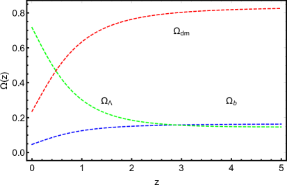
Figure 1: Dynamic evolution of the three energy-matter components of the Universe. One can observe the WDM domination and the domination of the running cosmological constant part for big and small redshifts $z$, respectively. The growing of DE as a consequence of baryons decay, it is also observed.

The solution for $\rho_{\Lambda}$ can be found by integrating (13),

$$\Omega_{\Lambda}(z)=B_{0}+\frac{\nu}{1-\nu}\,\left[\Omega_{r}(z)+\Omega_{dm}(z)+\Omega_{k}^{0}\,z(z+2)\right],$$ (22)

where

$$B_{0}\,=\,\Omega_{\Lambda}^{0}-\frac{\nu}{1-\nu}\,\big{(}\Omega_{r}^{0}+\Omega_{dm}^{0}\big{)}.$$ (23)

Finally, for the square of the Hubble parameter we find

$$\left(\frac{H(z)}{H_{0}}\right)^{2} = 1+\left(\Omega_{b}^{0}+\frac{2\nu\Omega_{k}^{0}}{2-\zeta}\right)\left[\frac{(1+z)^{\zeta}-1}{1-\nu}\right]+\Omega_{k}^{0}(z^{2}+2z)\left[1-\frac{\nu\zeta}{(1-\nu)(2-\zeta)}\right]$$ (24)

$$+ \frac{\Omega_{dm}^{0}}{1-\nu}\left\{\left[\nu+\frac{\nu\zeta}{3-\zeta}\,\,\frac{{}_{2}F_{1}(\alpha,\beta;\gamma;-b^{2})}{\sqrt{1+b^{2}}}\right](1+z)^{\zeta}-1\right\}$$

$$+ \frac{\Omega_{dm}^{0}(1+z)^{3}}{\sqrt{1+b^{2}}}\Big{[}\sqrt{1+b^{2}(1+z)^{2}}-\frac{\nu\zeta}{(1-\nu)(3-\zeta)}\,\,{}_{2}F_{1}(\alpha,\beta;\gamma;Z)\Big{]}.$$

In the limits of $\nu\to 0$ and $b\to 0$ we recover the standard $\Lambda$CDM model and in the case of $\omega=0$ and $\Omega_{dm}^{0}=0$ (that is, without WDM), we recover exactly the result presented in [20]. In Figure 1 is presented the cosmic evolution of the relative energy densities for normal matter, running vacuum and warm dark matter with respect to redshift $z$.

3 Cosmic perturbations

Let us consider the cosmological perturbations in the RRG with running $\rho_{\Lambda}$, following the approach developed in Refs. [20] and [32]. The first observation is that the perturbation of the WDM pressure should be derived from the equation of state (2),

$$\delta p_{dm}\,=\,\frac{\delta\rho_{dm}}{3}\Big{[}1-\Big{(}\frac{mc^{2}}{\varepsilon}\Big{)}^{2}\Big{]}\,=\,\frac{\delta\rho_{dm}(1-s)}{3}.$$ (25)

Taking the main feature of the RRG, this means that perturbations satisfy the same relation between pressure and energy density that the background quantities. The metric perturbations are defined by

$$g_{\mu\nu}=\bar{g}_{\mu\nu}+h_{\mu\nu},$$ (26)

with the associated Christoffel symbol

$$\Gamma^{\rho}_{\mu\nu}=\bar{\Gamma}^{\rho}_{\mu\nu}+\frac{1}{2}g^{\rho\lambda}\left(\partial_{\mu}h_{\lambda\nu}+\partial_{\nu}h_{\lambda\mu}-\partial_{\lambda}h_{\mu\nu}-2h_{\lambda\kappa}\bar{\Gamma}^{\kappa}_{\mu\nu}\right),$$ (27)

where the background quantities are marked by bars. E.g., the background metric has the form

$$\bar{g}_{\mu\nu}\,=\,\,\mbox{diag}\,\big{\{}1,-a^{2}(t)\delta_{ij}\big{\}}.$$ (28)

In the synchronous gauge $h_{0\mu}=0$, the $(00)$ component of the Ricci tensor is

$$R_{00}=\bar{R}_{00}+\delta R_{00},$$ (29)

where

$$\delta R_{00}\,=\,\frac{1}{2}\,\dot{h}+Hh\qquad\mbox{and}\qquad h\,=\,\frac{\partial}{\partial t}\Big{(}\frac{h_{ii}}{a^{2}}\Big{)}.$$ (30)

Perturbing the Einstein equations, we obtain

$$\delta R^{\mu}_{\nu}\,=\,8\pi G\left(\delta T_{\nu}^{\mu}-\frac{1}{2}Tg^{\rho\mu}\delta g_{\rho\nu}-\frac{1}{2}\delta T\delta^{\mu}_{\nu}\right),$$ (31)

where the total energy-momentum tensor $T_{\mu\nu}$ and its trace $T$ are given by Eq. (8).

It proves useful introducing the quantities

$$f_{1}(z)=\frac{\rho_{b}(z)}{\rho_{t}(z)},\qquad f_{2}(z)=\frac{\rho_{\Lambda}(z)}{\rho_{t}(z)},\qquad f_{3}(z)=\frac{\rho_{dm}(z)}{\rho_{t}(z)},$$ (32)

and

$$g(z)=\frac{2\nu H(z)}{3H^{2}(z)-3H_{0}^{2}\Omega_{k}^{0}(1+z)^{2}},$$ (33)

where $\rho_{t}$ is the total energy density. Thus, we arrive at the $00$-component of the linearized Einstein equations,

$$h^{\prime}-\frac{2h}{1+z}\,=\,-\frac{2\nu}{(1+z)g}\big{[}(1+3w)f_{1}\delta_{b}-2f_{2}\delta_{\Lambda}+(2-s)f_{3}\delta_{dm}\big{]},$$ (34)

where

$$\delta_{i}=\frac{\delta\rho_{i}}{\rho_{i}}\,.$$ (35)

is the relative density variation.

It is useful to denote

$$v=f_{1}\nabla_{i}(\delta V^{i})\qquad\mbox{and}\qquad u=f_{3}\nabla_{i}(\delta U^{i})$$ (36)

the divergences of the peculiar velocities. The time and spatial components of the perturbations satisfy the linear equations

$$\delta_{b}^{\prime}\,+\,\Big{[}\frac{f_{1}^{\prime}}{f_{1}}-\frac{3(1+w)f_{2}}{1+z}+\frac{(1-s-3w)f_{3}}{1+z}\Big{]}\delta_{r}\,-\,\frac{1+w}{(1+z)H}\Big{(}\frac{v}{f_{1}}-\frac{h}{2}\Big{)}$$

$$\,\,\quad=\,-\,\frac{1}{f_{1}}(\delta_{\Lambda}f_{2})^{\prime}\,-\,\frac{3(1+w)f_{2}}{1+z}\Big{[}1+\frac{(4-s)f_{3}}{3(1+w)f_{1}}\Big{]}\delta_{\Lambda},$$ (37)

$$v^{\prime}+\frac{[3(1+w)f_{1}+(4-s)f_{3}-5]}{1+z}\,v\,=\,\frac{k^{2}(1+z)}{(1+w)H}\left(f_{2}\delta_{\Lambda}-wf_{1}\delta_{b}\right),$$ (38)

$$\delta^{\prime}_{dm}+\Big{\{}\,\frac{f_{3}^{\prime}}{f_{3}}+\frac{3(1+w)f_{1}+(s-4)(f_{1}+f_{2})}{1+z}\Big{\}}\delta_{dm}\,+\,\frac{4-s}{3H(1+z)}\Big{(}\frac{h}{2}-\frac{u}{f_{3}}\Big{)}\,=\,0,\mbox{\quad}\mbox{\qquad}$$ (39)

$$u^{\prime}+\Big{[}\frac{3(1+w)f_{1}+(4-s)f_{3}-5}{1+z}-\frac{s^{\prime}}{4-s}\Big{]}u+\frac{k^{2}(1+z)f_{3}}{H}\Big{(}\frac{1-s}{4-s}\Big{)}\delta_{dm}\,=\,0.\mbox{\qquad\quad}$$ (40)

Perturbing Eq. (11), we get

$$\delta_{\Lambda}=\frac{g}{f_{2}}\Big{(}\frac{v}{f_{1}}-\frac{h}{2}\Big{)}.$$ (41)

It is easy to note that this equation is not dynamical, representing a constraint that should be used in other equations. Using (41) in Eqs. (34), (37) and (38), and rewriting the equations in the Fourier space, we arrive at the equations

$$h^{\prime}+\frac{2(\nu-1)}{1+z}\,h=\frac{2\nu}{1+z}\Big{[}\frac{2v}{f_{1}}-(1+3w)\frac{f_{1}}{g}\delta_{b}-(2-s)\frac{f_{3}}{g}\delta_{dm}\Big{]},$$ (42)

$$\delta_{b}^{\prime}+\Big{[}\frac{f_{1}^{\prime}}{f_{1}}-\frac{3(1+w)f_{2}}{1+z}+\frac{(1-s-3w)f_{3}}{1+z}\Big{]}\delta_{b}=\frac{1}{f_{1}}\Big{(}\frac{gh}{2}-\frac{gv}{f_{1}}\Big{)}^{\prime}\mbox{\qquad}$$

$$\qquad+\,\frac{1+w}{1+z}\Big{[}3g+\frac{(4-s)gf_{3}}{(1+w)f_{1}}-\frac{1}{H}\Big{]}\Big{(}\frac{h}{2}-\frac{v}{f_{1}}\Big{)},$$ (43)

$$v^{\prime}+\Big{\{}\frac{[3(1+w)f_{1}+(4-s)f_{3}-5]}{1+z}-\frac{k^{2}g(1+z)}{(1+w)Hf_{1}}\Big{\}}v$$

$$\qquad=\,-\frac{k^{2}g(1+z)}{2(1+w)H}\Big{(}h+\frac{2wf_{1}}{g}\,\delta_{b}\Big{)}.$$ (44)

Thus, the closed set of perturbation equations is given by (39), (40), (42), (3) and (3).

4 Some observational constraints

Let us use the equations calculated above and some of the available observational data to constrain the parameters of our model, including $\nu$, $b$ and $\Omega_{k}^{0}$.

4.1 Supernovae Ia

In this subsection we will use the data from Supernovas Ia called “Pantheon” sample [38], which is the largest combined sample of SNIa and consists of $1048$ data with the redshifts in the range $0.01<z<2.3$. It is a collection of the SNe Ia, discovered by the Pan-STARRS1 (PS1) Medium Deep Survey and SNe Ia from Low-z, SDSS, SNLS and HST surveys. This supernova Ia compilation uses The SALT 2 program to transform light curves into distances using a modified version of the Tripp formula [57],

$$\mu=m_{B}-M+\alpha x_{1}-\beta c+\Delta_{M}+\Delta_{B},$$ (45)

where $\mu$ is the distance modulus, $\Delta_{M}$ is a distance correction based on the host-galaxy mass of the SNIa and $\Delta_{B}$ is the distance correction based on predicted bias from simulations. Also, $\alpha$ is the coefficient of the relation between luminosity and stretch; $\beta$ is the coefficient of the relation between luminosity and color and $M$ is the absolute $B$-band magnitude of the fiducial SNIa with $x_{1}=0$ and $c=0$. Also $c$ is the color and $x_{1}$ is the light-curve shape parameter and $m_{B}$ is the log of the overall flux normalization. A covariance matrix $\bf{C}$ is defined such that

$$\chi_{SNIa}^{2}\,=\,\Delta{\bf\mu}^{T}\cdot\mathbf{C}^{-1}\cdot\Delta{\bf\mu},$$ (46)

where $\Delta{\bf\mu}={\bf\mu}_{obs}-{\bf\mu}_{model}$ and ${\bf\mu}_{model}$ is a vector of distance modulus from a given cosmological model and ${\bf\mu}_{obs}$ is a vector of observational distance modulus. The ${\bf\mu}={\bf m}-M$, where $M$ is the absolute magnitude and ${\bf m}$ is the apparent magnitude, which is is given by

$${\bf m}_{model}\,=\,M+5Log_{10}\big{(}D_{L}\big{)}\,+\,5Log_{10}\Big{(}\frac{c/H_{0}}{1Mpc}\Big{)}\,+\,25\,=\,\bar{M}+25+5Log\big{(}D_{L}\big{)},\mbox{\quad}$$ (47)

where $D_{L}=\frac{H_{0}}{c}d_{L}$ and $\bar{M}=M+5Log(\frac{c/H_{0}}{1Mpc})$ is an nuisance parameter, which depends on the Hubble constant $H_{0}$ and the absolute magnitude $M$. To minimize with respect to the nuisance parameter we follow a process similar to Refs. [58, 59]. Therefore, the $\chi^{2}_{\bar{M}marg}$ is,

$$\chi^{2}_{\bar{M}marg}\,=\,\tilde{a}+\log\Big{(}\frac{\tilde{e}}{2\pi}\Big{)}-\frac{\tilde{b}^{2}}{\tilde{e}},$$ (48)

where

$$\tilde{a}=\Delta{\bf m}^{T}\cdot C^{-1}\cdot\Delta{\bf m},\qquad\tilde{b}=\Delta{\bf m}^{T}\cdot C^{-1}\cdot\mathbb{I},\qquad\tilde{e}=\mathbb{I}^{T}\cdot C^{-1}\cdot\mathbb{I}.$$ (49)

Here $\Delta{\bf m}={\bf m}_{obs}-{\bf m}_{model}$ and $\mathbb{I}$ is the identity matrix.

4.2 Power Spectrum

The numerical analysis of the perturbations in our model can be confronted with the power spectrum data of the BOSS-DR11 project [39]. For the comparison of these data with the theoretical model described in the previous section, we use the chi-square statistics,

$$\chi^{2}_{DR11}=\sum_{i=1}^{n=37}{\frac{\big{[}P_{the}(z_{obs,i},k,\Omega^{0}_{dm},\Omega^{0}_{k},b,\nu)-P_{obs,i}\big{]}^{2}}{\sigma^{2}_{obs,i}}},$$ (50)

where $P$ denotes the power spectrum and we used the Planck collaboration value $\Omega^{0}_{b}=0.049$ [2] and $H_{0}=70\frac{km/s}{Mpc}$. In our case, the theoretical power spectrum, $(P_{the})$, results from the solution of the coupled system of Eqs. (39), (40) and (42)-(3). Namely, the power spectrum of the normal (baryonic) matter at the current redshift is determined as

$$P(k)=\big{|}\delta_{b}(k)\big{|}^{2}.$$ (51)

Solving system of equations (39), (40), (42), (3) and (3) requires specifying the initial conditions for all the variables. For this end, we follow Ref. [33] and assume the transfer function BBKS [60, 61], given by the expression

$$T(z)=\frac{\,\mbox{ln}\,{(1+2.34q)}}{2.34q}\left(1+3.89q+16.1q^{2}+5.64q^{3}+6.71q^{4}\right)^{-1/4},$$ (52)

where

$$q(k)=\frac{k}{h\Sigma\,Mpc^{-1}}$$ (53)

and

$$\Sigma\,=\,\Omega^{0}_{m}h\,\exp\Big{(}-\Omega^{0}_{b}-\sqrt{2h}\frac{\Omega^{0}_{b}}{\Omega^{0}_{m}}\Big{)},$$ (54)

where $\Omega^{0}_{m}=\Omega^{0}_{dm}+\Omega^{0}_{b}$ and $h=H_{0}/(100\,\,km{}\,s^{-1}\,Mpc^{-1})$.

Parameters	Best-fitting
$\Omega^{0}_{dm}$	$0.249\pm 0.107$
$\Omega^{0}_{k}$	$-0.05\pm 0.120$
$b$	$0.000655\pm 0.000300$
$\nu$	$0.000407\pm 0.000070$

Table 1: Best-fitting parameters for $1\sigma$ confidence intervals and for the $\chi^{2}_{total}$ including the SNIa and DR11 data sets.

The first results of the numerical analysis can be seen in Table 1.

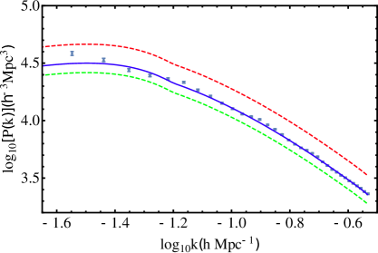
Figure 2: Reconstruction of the power spectrum (PS) of matter from the solution of the system of equations (39), (40), (42), (3) and (3). The blue line is constructed with the best fitting from Table 1. The green and red dashed lines correspond to the values of $b=10^{-3}$ and $\nu=10^{-3}$, respectively, letting fixed all the other values. It is evident that the matter PS is quite sensible to $\nu$ and $b$ values. On the other hand, no essential changes under variation of $\Omega^{0}_{k}$ were observed.

The plot for the power spectrum which results from the approach explained above, is shown in Figure 2. The blue line is calculated using the best fitting given by the Table 1. The other lines keep all the parameters fixed while varying the parameter of the running $\nu$ (red line) or the warmness $b$ (green line).

To determine the observational constraints using the two data sets described above, namely SNIa and matter power spectrum DR11, we define the total $\chi^{2}$ as the sum of the individual contributions, in the form

$$\chi^{2}_{total}=\chi^{2}_{SNIa}+\chi^{2}_{DR11}$$ (55)

and elaborate this value using the data presented in this section. The results of this treatment are illustrated in Fig. 3, where we show how the parameters that characterize our model vary with respect to the curvature $\Omega^{0}_{k}$. One can observe that the two data sets are complementary, except the case of the plane $(\Omega^{0}_{k},b)$.

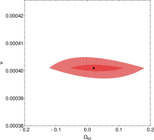
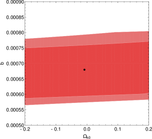
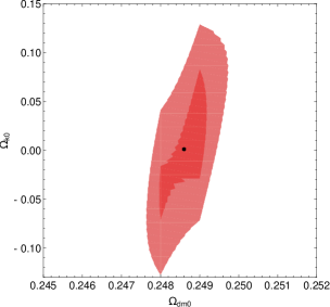
Figure 3: Observational constraints of the curvature parameter $\Omega^{0}_{k}$ versus the free parameters of the model ($\Omega^{0}_{dm}$, $b$, $\nu$), based on $\chi^{2}_{total}$. In the top figure on the right we show the degeneracy on $\Omega^{0}_{k}$ versus $b$. In the top figure on the left side there are constraints with respect to parameter $\nu$ and at the bottom we show constraints with respect to parameter $\Omega^{0}_{dm}$. In all cases we assume $H_{0}=70\frac{km/s}{Mpc}$ and $\Omega^{0}_{b}=0.049$.

5 Conclusions

We have developed a cosmological model with a non-zero spatial curvature, running cosmological constant and warm Dark Matter (WDM). The WDM is described in terms of the RRG model and the form of the hypothetical running of $\rho_{\Lambda}$ is fixed by the arguments of covariance of the effective action of vacuum. The ideal fluid describing normal matter assume a general equation of state with a constant $\omega$. At the background level, we have found the analytical and general expressions for the corresponding relative energy densities, as well as the expansion rate given by the Hubble parameter.

The analysis of density perturbations for all involved fluids leads to the system of equations for the density contrasts. The new element compared to the previous works [20, 33, 35] is that this time we took into account modifications caused by the spatial curvature, including on the expansion rate. This system of equations has been solved numerically to reconstruct the corresponding matter power spectrum and to impose the restrictions on the free parameters of our model, such as the running parameter $\nu$ and the warmness $b$, taking into account the effect of the spatial curvature $\Omega^{0}_{k}$.

Once we include spatial curvature, the observational constraints restrict the magnitudes of both parameters $\nu$ and $b$ at the order of $10^{-4}$. The combined data prefers a relatively low warm dark matter component of the order of $\Omega^{0}_{dm}=0.25$, as a component of the total matter balance today, $\Omega^{0}_{m}=\Omega^{0}_{dm}+\Omega^{0}_{b}=0.299$. However, there is a degeneracy in the observational constraints on the parameter $\Omega^{0}_{k}$, which can be clearly observed in the diagram showing the plane $(\Omega^{0}_{k},b)$ in Fig. 3. Even though, a slight preference for a closed universe can be identified.

In conclusions, adding the curvature parameter to our model of running cosmological constant with WDM, increases the number of dimensions of the parameter space, regardless the effect of space curvature is phenomenologically not very strong. Additional tests may be useful to obtain more robust constraints on the parameters $\nu$ and $b$. In particular, we expact that the observational constraints coming from CMB and BAO may give a strong enforcements of our results. The theoretical basis of these tests would be a natural continuation of the present work.

On the other hand, considering the generality of the model and its ability to describe different phases of the Universe, another possible perspective for further investigations work could be to study the Hubble tension by including the parameter $w$, defined in Eq. (1), as a new free parameter and estimating the Hubble parameter today. We consider this possibility for a possible future works.

References

- [1]
- [2] N. Aghanim et al., Planck 2018 results. VI. Cosmological parameters, arXiv:1807.06209.
- [3] L. Anderson, et al. “The clustering of galaxies in the SDSS-III Baryon Oscillation Spectroscopic Survey: baryon acoustic oscillations in the Data Releases 10 and 11 Galaxy samples,” Monthly Notices of the Royal Astronomical Society 441.1 24 (2014).
- [4] S. Weinberg, “The cosmological constant problem,” Rev. Mod. Phys. 61 1 (1989).
- [5] S. Weinberg, “Anthropic bound on the cosmological constant,” Phys. Rev. Lett. 59 2607 (1987).
- [6] I.L. Shapiro, J. Solà, “Scaling behavior of the cosmological constant: Interface between quantum field theory and cosmology,” JHEP 02 006 (2002).
- [7] I.L. Shapiro, “Effective Action of Vacuum: Semiclassical Approach,” Class. Quant. Grav. 25 103001 (2008).
- [8] V. Sahni and A.A. Starobinsky. “The case for a positive cosmological -term,” Int. Journ. Mod Phys. D9 373 (2000).
- [9] P.J.E. Peebles and B. Ratra, “The cosmological constant and dark energy,” Rev. Mod. Phys. 75 559 (2003).
- [10] V. Sahni and A. Starobinsky, “Reconstructing Dark Energy,” Int. J. Mod. Phys. D15 2105 (2006).
- [11] G. Bertone, D. Hooper and J. Silk, “Particle dark matter: Evidence, candidates and constraints,” Phys. Repts. 405 279 (2005).
- [12] M. Tegmark et al., “The three-dimensional power spectrum of galaxies from the sloan digital sky survey,” The Astrophysical Journal 606 702 (2004).
- [13] N. Aghanim et al., Planck 2018 results. V. CMB power spectra and likelihoods, arXiv:1907.12875.
- [14] S. Capozziello and M. De Laurentis, “Extended theories of gravity,” Phys. Repts. 509 167 (2011).
- [15] I.L. Buchbinder, S.D. Odintsov and I.L. Shapiro, Effective action in quantum gravity, (IOP Publishing, Bristol, 1992).
- [16] T. Taylor and G. Veneziano, “Quantum gravity at large distances and the cosmological constant,” Nucl. Phys. B 345, 210 (1990).
- [17] B.L. Giacchini, T. de Paula Netto and I.L. Shapiro, On the Vilkovisky unique effective action in quantum gravity, arXiv:2006.04217.
- [18] I.L. Shapiro, J. Solà, “On the possible running of the cosmological ‘constant’,” Phys. Lett. B682 105 (2009).
- [19] I.L. Shapiro, J. Solà, C. España-Bonet, P. Ruiz-Lapuente, “Variable cosmological constant as a Planck scale effect,” Phys. Lett. 574B 149 (2003).
- [20] J. C. Fabris, I. L. Shapiro, J. Solà, “Density Perturbations for Running Cosmological Constant,” JCAP 0702 016 (2007).
- [21] I. L. Shapiro, J. Solà and H. Stefancic, “Running and at low energies from physics at MX: possible cosmological and astrophysical implications,” JCAP 0501 012 (2005).
- [22] J. Grande, J. Solà, J.C. Fabris and I.L. Shapiro, “Cosmic perturbations with running G and Lambda,” Class. Quantum Grav. 27 105004 (2010).
- [23] J. Solà “Cosmological constant and vacuum energy: old and new ideas,” Journal of Physics: Conference Series. 453 (IOP Publishing, 2013).
- [24] E.L.D. Perico and D.A. Tamayo, “Running vacuum cosmological models: linear scalar perturbations,” JCAP 1708 026 (2017).
- [25] S. Basilakos, N. E. Mavromatos and J. Solà, “Gravitational and chiral anomalies in the running vacuum universe and matter-antimatter asymmetry,” Phys. Rev. D101 045001 (2020).
- [26] S. Hannestad and R. J. Scherrer, “Self-interacting warm dark matter,” Phys. Rev. D62 043522 (2000).
- [27] P. Bode J. P. Ostriker and N. Turok, “Halo formation in warm dark matter models,” The Astrophysical Journal 556 93 (2001).
- [28] M. Viel, J. Lesgourgues, M. G. Haehnelt, S. Matarrese and A. Riotto, “Constraining warm dark matter candidates including sterile neutrinos and light gravitinos with WMAP and the Lyman- forest,” Phys. Rev. D71 063534 (2005).
- [29] A.D. Sakharov, “The initial stage of an expanding universe and the appearance of a nonuniform distribution of matter,” Sov. Phys. JETP 22 241 (1966).
- [30] G. de Berredo-Peixoto, I. L. Shapiro and F. Sobreira, “Simple cosmological model with relativistic gas,” Mod. Phys. Lett.A20 2723 (2005).
- [31] F. Jüttner, “Die dynamik eines bewegten gases in der relativtheorie,” Annalen der Physik 6 145 (1911).
- [32] J. C. Fabris, I. L. Shapiro and F. Sobreira, “DM particles: how warm they can be?” JCAP 0902 001 (2009).
- [33] J. C. Fabris, I. L. Shapiro and A. M. Velasquez-Toribio, “Testing dark matter warmness and quantity via the reduced relativistic gas model,” Phys. Rev. D85 023506 (2012).
- [34] W. S. Hipólito-Ricaldi, R. F. Marttens, J. C. Fabris, I. L. Shapiro and L. Casarini, “On general features of warm dark matter with reduced relativistic gas,” Eur. Phys. J. C 78 365 (2018).
- [35] J.A. Agudelo Ruiz, T. de Paula Netto, J.C. Fabris and I.L. Shapiro, Primordial universe with the running cosmological constant, arXiv:1911.06315; to appear in Eur. Phys. J. C.
- [36] Ya.B. Zeldovich and A.A. Starobinsky, “Particle production and vacuum polarization in an anisotropic gravitational field,” Sov. Phys. JETP 34 1159 (1972) [Zh. Eksp. Teor. Fiz. 61 2161 (1971)].
- [37] A. Dobado and A.L. Maroto, “Particle production from nonlocal gravitational effective action,” Phys. Rev. D60 104045 (1999).
- [38] D. M. Scolnic et al., “The complete light-curve sample of spectroscopically confirmed SNe Ia from Pan-STARRS1 and cosmological constraints from the combined pantheon sample,” The Astrophysical Journal 859 101 (2018).
- [39] L. Anderson et al., “The clustering of galaxies in the SDSS-III Baryon Oscillation Spectroscopic Survey: baryon acoustic oscillations in the Data Releases 10 and 11 Galaxy samples,” Monthly Notices of the Royal Astronomical Society 441 24 (2014).
- [40] J. Ooba, B. Ratra and N. Sugiyama, “Planck 2015 constraints on the non-flat CDM inflation model,” The Astrophysical Journal 864 80 (2018).
- [41] J. Ooba, B. Ratra and N. Sugiyama, “Planck 2015 constraints on the non-flat XCDM inflation model,” The Astrophysical Journal 869 34 (2018).
- [42] J. Ooba, B. Ratra and N. Sugiyama, “Planck 2015 Constraints on the Nonflat CDM Inflation Model,” The Astrophysical Journal 866 68 (2018).
- [43] C. Park and B. Ratra, “Observational Constraints on the Tilted Spatially Flat and the Untilted Nonflat CDM Dynamical Dark Energy Inflation Models,” The Astrophysical Journal 868 83 (2018).
- [44] C. Park and B. Ratra, “Observational constraints on the tilted flat-XCDM and the untilted nonflat XCDM dynamical dark energy inflation parameterizations,” Astrophysics and Space Science 364 82 (2019).
- [45] A.M. Velasquez-Toribio and A. dos R. Magnago, “Observational constraints on the non-at CDM model and a null test using the transition redshift,” EPJC 80 562 (2020).
- [46] J. Ryan, S. Doshi and B. Ratra, “Constraints on dark energy dynamics and spatial curvature from Hubble parameter and baryon acoustic oscillation data,” Monthly Notices of the Royal Astronomical Society 480 759 (2018).
- [47] J. Ryan, Y. Chen and B. Ratra, “Baryon acoustic oscillation, Hubble parameter, and angular size measurement constraints on the Hubble constant, dark energy dynamics, and spatial curvature,” Monthly Notices of the Royal Astronomical Society 488 3844 (2019).
- [48] C. Park and B. Ratra, “Using SPTpol, Planck 2015, and non-CMB data to constrain tilted spatially-flat and untilted non-flat CDM, XCDM, and CDM dark energy inflation cosmologies,” Phys. Rev. D101 083508 (2020).
- [49] W. Handley “Primordial power spectra for curved inflating universes,” Phys. Rev. D100 123517 (2019).
- [50] S. Castardelli dos Reis and I.L. Shapiro, “Cosmic anisotropy with Reduced Relativistic Gas,” Eur. Phys. J. C78 145 (2018).
- [51] G. Pordeus-da-Silva, R. Batista and L. Medeiros, “Theoretical foundations of the reduced relativistic gas in the cosmological perturbed context,” JCAP 06 043 (2019).
- [52] N.R. Bertini, W.S. Hipólito-Ricaldi, F. de Melo-Santos and D.C. Rodrigues, “Cosmological framework for renormalization group extended gravity at the action level,” Eur. Phys. J. C80 479 (2020).
- [53] A.A. Starobinski, “A new type of isotropic cosmological models without singularity,” Phys. Lett. B91 99 (1980).
- [54] A.A. Starobinsky, “The perturbation spectrum evolving from a nonsingular initially de-Sitter cosmology and the microwave background anisotropy,” Sov. Astron. Lett. 9 302 (1983).
- [55] E.V. Gorbar, I.L. Shapiro, “Renormalization Group and Decoupling in Curved Space.” JHEP 02 021 (2003).
- [56] E. Belgacem, Y. Dirian, S. Foffa and M. Maggiore, “Nonlocal gravity. Conceptual aspects and cosmological predictions,” JCAP 1803 002 (2018).
- [57] R. Tripp, “A two-parameter luminosity correction for Type IA supernovae,” Astronomy and Astrophysics 331 815 (1998).
- [58] A. Conley et al., “Supernova constraints and systematic uncertainties from the first three years of the supernova legacy survey,” The Astrophysical Journal Supplement Series 192 1 (2010).
- [59] R. Arjona, W. Cardona and S. Nesseris, “Unraveling the effective fluid approach for f (R) models in the subhorizon approximation,” Phys. Rev. D99 043516 (2019).
- [60] A. M. Velasquez-Toribio, “Cosmological Perturbations and the Running Cosmological Constant Model,” Int. Journ. Mod. Phys. D21 1250026 (2012).
- [61] J. M. Bardeen et al., “The statistics of peaks of Gaussian random fields,” The Astrophysical Journal 304 15 (1986).