Efficiency of Local Learning Rules in Threshold-Linear Associative Networks

Abstract

We derive the Gardner storage capacity for associative networks of threshold linear units, and show that with Hebbian learning they can operate closer to such Gardner bound than binary networks, and even surpass it. This is largely achieved through a sparsification of the retrieved patterns, which we analyze for theoretical and empirical distributions of activity. As reaching the optimal capacity via non-local learning rules like backpropagation requires slow and neurally implausible training procedures, our results indicate that one-shot self-organized Hebbian learning can be just as efficient.

I Introduction

Learning in neuronal networks is believed to happen largely through changes in the weights of the synaptic connections between neurons. Local learning rules, those that self-organize through weight changes depending solely on the activity of pre- and postsynaptic neurons, are generally considered to be more biologically plausible than nonlocal ones Brown et al. (1990); *hebb1949organization; *Ami92book. But how effective are local learning rules? Quite ineffective, has been the received wisdom since the 80’s, when nonlocal iterative algorithms came to the fore. However, this wisdom, when it comes to memory storage and retrieval, is largely based on analysing networks of binary neurons Hopfield (1982); Amit et al. (1987); Derrida et al. (1987); Gardner (1988), while neurons in the brain are not binary.

A better, but still mathematically simple description of neuronal input-output transformation is through threshold-linear (TL) activation function Hartline and Ratliff (1957); *Har+58; Treves (1990a), also predominantly adopted in recent deep learning applications (called ReLu in that context) Nair and Hinton (2010); *maas2013rectifier; *he2015delving; *goodfellow2016deep. Therefore, one may ask if the results from the 80’s highlighting the contrast between the effective, iterative procedures used in machine learning and the self-organized, one-shot, perhaps computationally ineffective local learning rules are valid beyond binary units Pereira and Brunel (2018).

The Hopfield model, a most studied model of memory, is a fully connected network of $N$ binary units endowed with a local, Hebbian learning rule Hopfield (1982); Amit et al. (1987): the weight between two units increases if they have the same activity in a memory pattern; otherwise it decreases. The network can retrieve only up to $p_{max}\simeq 0.14N$ patterns, while, in comparison, Elisabeth Gardner showed Gardner (1988) that with $C$ connections per unit, the optimal capacity that such a network can attain is $p_{max}=2C$, about 14 times higher; the bound can be approached through iterative procedures like backpropagation that progressively reduce the difference between current and desired output. This consolidated the impression that unsupervised, Hebbian plasticity may well be of biological interest, but is rather inefficient for memory storage. In the fully connected Hopfield model, the transition to no-retrieval is discontinuous: right below the storage capacity, $\sim 1.5\%$ of units in a retrieved pattern are misaligned with the stored pattern, but $50\%$, i.e., chance level, just above the capacity Amit et al. (1987). This rather low error certainly contributes to the low capacity. However, the negative characterization of Hebbian learning in binary networks persisted even when more errors occur: in the more biologically relevant highly diluted networks the error smoothly goes to $50\%$ Gardner et al. (1989), but the capacity is still a factor of 3 away Derrida et al. (1987), approaching the bound only when the fraction of active unit in each pattern is $f\ll 1$ Tsodyks and Feigel’man (1988).

What about TL units? Are they more efficient in the unsupervised learning of memory patterns? Here we study the optimal pattern capacity à la Gardner in networks of TL units. Past work discussed above Tsodyks and Feigel’man (1988) had suggested that the distribution of activity (along with the connectivity) may play a role in how efficient Hebbian learning is, but, back then, this only meant changing $f$. Besides being a better model of neuronal input-output transformation, by allowing non-binary patterns, TL units permit a better understanding of the interplay between the retrieval properties of recurrent networks and the distribution of the activity stored in the network. In fact, we show that while for binary patterns the Gardner bound is larger than the Hebbian capacity no matter how sparse the code, this does not, in general, hold for non-binary stored patterns: the Hebbian capacity can even surpass the bound. This perhaps surprising violation of the bound is because the Gardner calculation imposes an infinite output precision Bollé et al. (1993), while Hebbian learning exploits its loose precision to sparsify the retrieved pattern. In other words, with TL units, Hebbian capacity can get much closer to the optimal capacity or even surpass it, by retrieving a sparser version of the stored pattern. We find that experimentally observed distributions from the Inferior-Temporal (IT) visual cortex Treves et al. (1999), which can be taken as patterns to be stored, would be sparsified about $50\%$ by Hebbian learning, and would reach about $50\%-80\%$ of the Gardner bound.

II Model Description

We consider a network of $N$ units and $p$ patterns of activity, $\{\eta_{i}^{\mu}\}_{i=1,..,N}^{\mu=1,..,p}$ each representing one memory stored in the connection weights via some procedure. Each $\eta_{i}^{\mu}$ is drawn independently for each unit $i$ and each memory $\mu$ from a common distribution Pr($\eta$). The activity of unit $i$ is denoted by $v_{i}$ and is determined by the activity of the $C$ units feeding to it as

$$v_{i}=g[h_{i}-\vartheta]^{+}$$ (1a)

$$h_{i}\{v_{i}\}=\frac{1}{\sqrt{C}}\sum_{j}J_{ij}v_{j},$$ (1b)

where $[x]^{+}=x$ for $x>0$ and $=0$ otherwise; and both the gain $g$ and threshold $\vartheta$ are fixed parameters. The storage capacity, or capacity for short, is defined as $\alpha_{c}\equiv p_{\rm max}/C$, with $p_{max}$ the maximal number of memories that can be stored and individually retrieved. The synaptic weights $J_{ij}$ are taken to satisfy the spherical normalization condition for all $i$

$$\sum_{j\neq i}J_{ij}^{2}=C.$$ (2)

We are interested in finding the set of $J_{ij}$ that satisfy Eq. (2), such that patterns $\{\eta_{i}^{\mu}\}_{i=1,..,N}^{\mu=1,..,p}$ are self-consistent solutions of Eqs. (1), namely that for all $i$ and $\mu$ we have, $h_{i}^{\mu}=\vartheta+\eta_{i}^{\mu}/g$ if $\eta_{i}^{\mu}>0$ and $h_{i}^{\mu}\leq\vartheta$ if $\eta_{i}^{\mu}=0$.

III Replica Analysis

Adapting the procedure introduced in Gardner (1988) for binary units to our network, we evaluate the fractional volume of the space of the interactions $J_{ij}$ which satisfy Eqs. (1)-(2), using the replica trick and the replica symmetry ansatz, we obtain the standard order parameters $m=\frac{1}{\sqrt{C}}\sum_{j}J_{ij}$ and $q=\frac{1}{C}\sum_{j}J_{ij}^{a}J_{ij}^{b}$ corresponding, respectively, to the average of the weights within each replica and to their overlap between two replicas $a$ and $b$ (Suppl. Mat. at [URL], Sect. A). Increasing $p$, for $C\to\infty$, shrinks the volume of the compatible weights, eventually to a single point, i.e., when there is only a unique solution and the storage capacity is reached. This corresponds to the case where all the replicated weights are equal $q\to 1$, implying that only one configuration satisfying all the equations exists. Adding a further memory pattern would make it impossible, in general, to satisfy them all. At the end, we obtain the following equations for $\alpha_{c}$

$$0 = -f(x+\frac{d_{1}}{g\sqrt{d_{3}}})+(1-f)\int_{x}^{\infty}Dt(t-x)$$ (3)

$$\frac{1}{\alpha_{c}} = f\Big{[}x^{2}+\frac{d_{2}}{g^{2}d_{3}}+\frac{2xd_{1}}{g\sqrt{d_{3}}}+1\Big{]}+(1-f)\int_{x}^{\infty}Dt(t-x)^{2},$$

where we have introduced the averages over Pr($\eta$): $d_{1}\equiv\langle\eta_{i}^{\mu}\rangle$, $d_{2}\equiv\langle(\eta_{i}^{\mu})^{2}\rangle$ and $d_{3}\equiv d_{2}-d_{1}^{2}$; $x=(\vartheta-d_{1}m)/\sqrt{d_{3}}$ is the normalized difference between the threshold and the mean input, while $f={\rm Pr}(\eta>0)$ is the fraction of active units and $Dt\equiv dt\exp(-t^{2}/2)/\sqrt{2\pi}$. The two equations yield $x$ and $\alpha_{c}$. Both equations can be understood as averages over units, respectively of the actual input and of the square input, which determine the amount of quenched noise and hence the storage capacity.

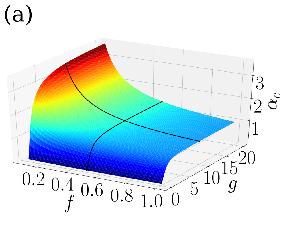
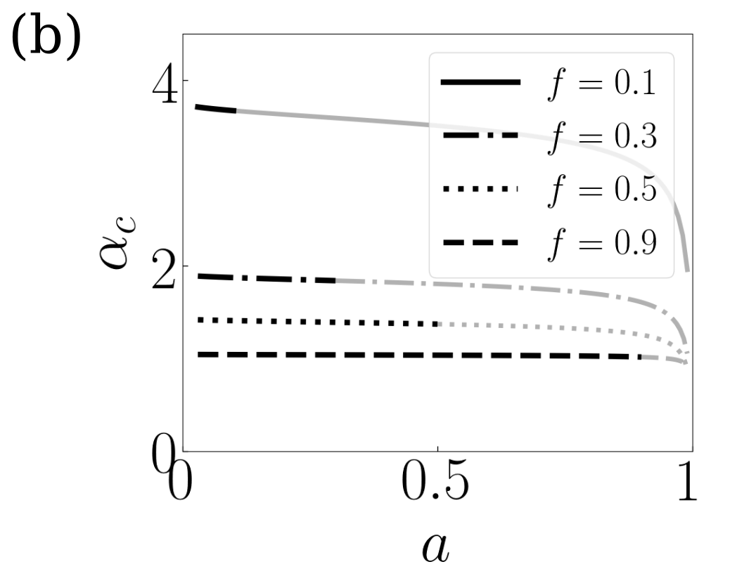
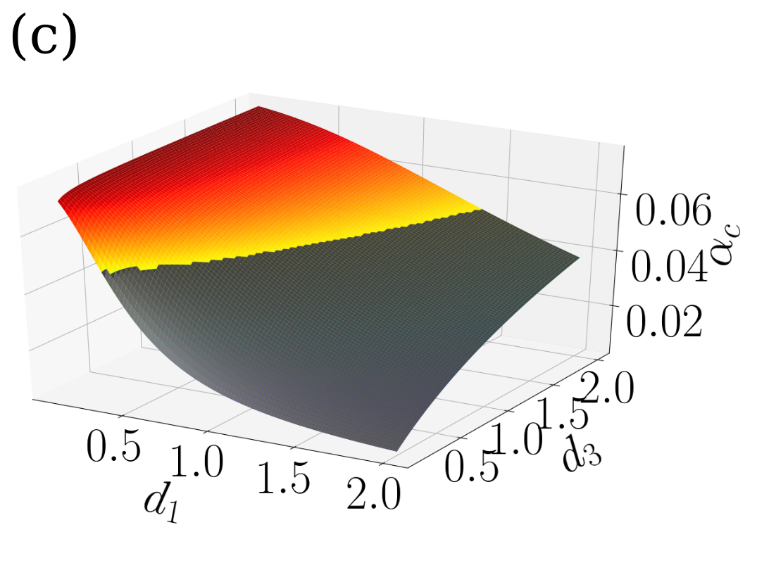
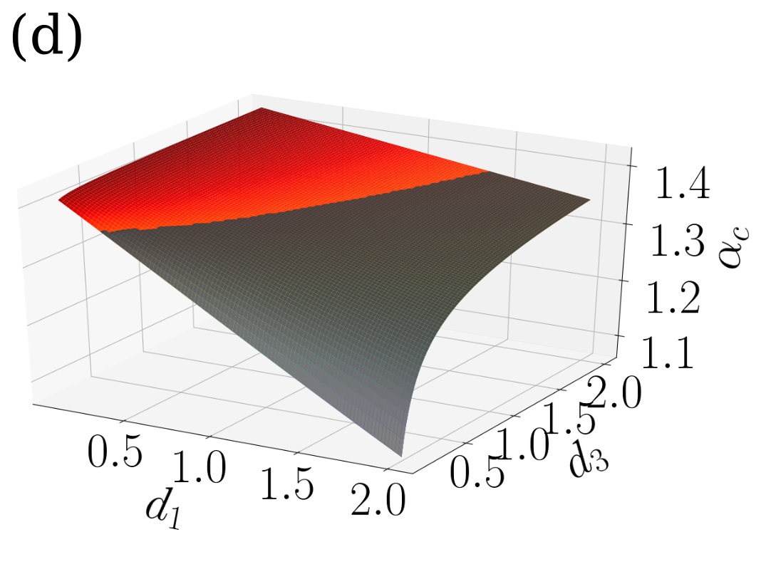
Figure 1: Dependence of the Gardner capacity $\alpha_{c}$ on different parameters: in (a) as a function of $g$ and $f$ ($d_{1}=1.1,d_{2}=2$), in (b) as a function of $a=d_{1}^{2}/d_{2}$ for different values of $f$ ($g=10$, $d_{1}=1.1$), in (c) and (d) as a function of $d_{1}$ and $d_{3}$ for $g=0.2$ and $g=10$, respectively ($f=0.5$). Note that fixing $f$ restricts the available range of $a$, as $a$ cannot be larger than $f$; the inaccessible ranges are shadowed in (b-d).

The capacity, $\alpha_{c}$, then depends on the proportion $f$ of active units, but also on the gain $g$, and on the cumulants $d_{1}$ and $d_{3}$. Fig. 1a shows that at fixed $g$, $\alpha_{c}$ increases as more and more units remain below threshold, ceasing to contribute to the quenched noise. In fact, $\alpha_{c}$ diverges as $[2f\ln(1/\sqrt{2\pi}f)]^{-1}$, for $f\to 0$; see Suppl. Mat. at [URL], Sect. B. At fixed $f$, there is an initially fast increase with $g$ followed by a plateau dependence for larger values of $g$. One can show that $\alpha_{c}\to\frac{g^{2}}{g^{2}+1}$ as $f\to 1$, i.e., when all the units in the memory patterns are above threshold, it is always $\alpha_{c}<1$ for any finite $g$. At first sight this may seem absurd: a linear system of $N^{2}$ independent equations and $N^{2}$ variables always has an inverse solution, which would lead to $\alpha_{c}$ being (at least) one. Similar to what was already noted in (Bollé et al., 1993), however, the inverse solution does not generally satisfy the spherical constraint in Eq. (2); but it does, in our case, in the limit $g\rightarrow\infty$ and this can also be understood as the reason why $\alpha_{c}$ is highest when $g$ is very large. In practice, Fig. 1 indicates that over a broad range of $f$ values, $\alpha_{c}$ approaches its $g\to\infty$ limit already for moderate values of $g$; while the dependence on $d_{1}$ and $d_{3}$ is only noticeable for small $g$, as can be seen by comparing Fig. 1c and d. For $g\to\infty$, one sees that Eqs. (3) depend on Pr($\eta$) only through $f$.

Eqs. (3), at $g\to\infty$, have been verified by explicitly training a threshold linear perceptron with binary patterns, evaluating $\alpha_{c}$ numerically as the maximal load which can be retrieved with no errors; See Suppl. Mat. at [URL], Sect. C for details. Estimated values of $\alpha_{c}$ are depicted by red diamonds in Fig. 2, and they follow the profile of the solid line describing the $g\to\infty$ limit of Eq. (3).

IV Comparison with a Hebbian Rule: theoretical analysis

With highly diluted connectivity and non-sparse patterns a binary network can get to $1/\pi$ of the bound, even if with vanishing overlaps, much closer than in the fully connected case. This is intuitively because the quenched noise is diminished as $J_{ij}$ and $J_{ji}$ become effectively independent. Besides its biological relevance, with TL units, the fair comparison to the capacity à la Gardner is thus that of a Hebbian network with highly diluted connectivity. In what follows, we indicate the Gardner capacity as calculated in the previous section and the Hebbian capacity, by $\alpha^{G}_{c}$ and $\alpha_{c}^{H}$, respectively, and use similar superscript notations for other quantities.

The capacity of the TL network with diluted connectivity was evaluated analytically in Treves (1991a); *Tre+91; see Suppl. Mat. at [URL], Sect. D for a recap, which includes Refs. Treves (1990b); *Rou+06. Whereas for $g\to\infty$ the Gardner capacity depends on Pr($\eta$) only via $f$, for Hebbian networks it does depend on the distribution, and most importantly on $a$, the sparsity

$$a=\langle\eta_{i}^{\mu}\rangle^{2}/\langle(\eta_{i}^{\mu})^{2}\rangle$$ (4)

whose relation to $f$ depends on the distribution Treves (1991a); *Tre+91.

Fig. 2 shows the results for 3 examples of binary, ternary and quaternary distributions for which $f$ and $a$ are related through $f=a$, $9a/5$ and $9a/4$, respectively, see Suppl. Mat. at [URL], Sect. E; the Hebbian and the Gardner capacities diverge in the sparse coding limit.

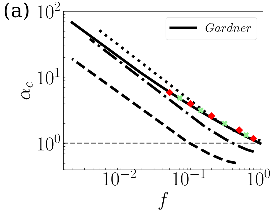
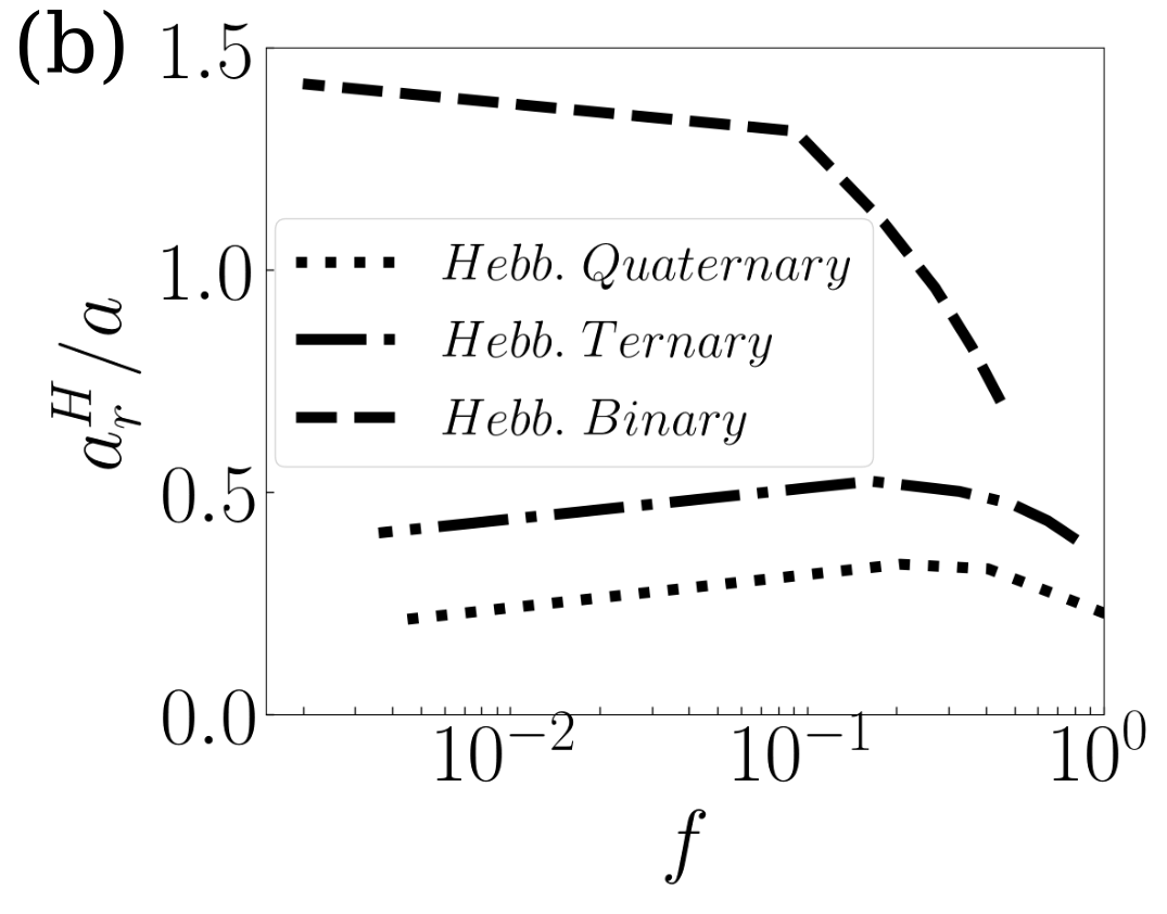
Figure 2: Hebbian vs Gardner capacity. (a) $\alpha_{c}^{H}$ vs. $f$ for different sample distribution of stored patterns compared to the analytically calculated universal $\alpha_{c}^{G}$; the red diamonds and green crosses are reached using perceptron training for binary and ternary patterns, respectively. (b) the sparsification of the stored patterns at retrieval, for Hebbian networks at their capacity.

When attention is restricted to binary patterns in Fig. 2a, the Gardner capacity, $\alpha^{G}_{c}$, seems to provide an upper bound to the capacity reached with Hebbian learning; more structured distributions of activity, however, dispel such a false impression: the quaternary example already shows higher capacity for sufficiently sparse patterns. The bound, in fact, would only apply to perfect errorless retrieval, whereas Hebbian learning creates attractors which are, up to the Hebbian capacity limit, correlated but not identical to the stored patterns; in particular, we notice that when considering TL units and Hebbian learning, in order to reach close to the capacity limit, the threshold has to be such as to produce sparser patterns at retrieval, in which only the units with the strongest inputs get activated. Fig. 2b shows the ratio of the sparsity of the retrieved pattern produced by Hebbian learning, $a^{H}_{r}=\langle v_{i}^{\mu}\rangle^{2}/\langle(v_{i}^{\mu})^{2}\rangle$ (estimated as described in Suppl. Mat. at [URL]) to that of the stored pattern $a$, vs. $f$: except for the binary patterns at low $f$, the retrieved patterns, at the storage capacity, are always sparser than the stored ones. The largest sparsification happens for quaternary patterns, for which the Hebbian capacity overtakes the Gardner bound, at low $f$. Sparser patterns emerge as, to reach close to $\alpha_{c}^{H}$, $\vartheta$ has to be such as to inactivate most of the units with intermediate activity levels in the stored pattern. Of course, the perspective is different if $\alpha_{c}^{H}$ is considered as a function of $a_{r}$ instead of $a$, in which case the Gardner capacity remains unchanged, as it implies retrieval with $a_{r}=a$, and is above $\alpha_{c}^{H}$ for each of the 3 sample distributions; see Fig. 1 of Suppl. Mat. at [URL].

V Comparison with a Hebbian Rule: experimental data

Having established that the Hebbian capacity of TL networks can surpass the Gardner bound for some distributions, we ask what would happen with distributions of firing rates naturally occurring in the brain. We considered published distributions of single neurons in IT cortex in response to short naturalistic movies Treves et al. (1999). Such distributions can be taken as examples of patterns elicited by visual stimuli, to be stored with Hebbian learning, given appropriate conditions, and later retrieved using attractor dynamics, triggered by a partial cue Fuster and Jervey (1981); *miyashita1988neuronal; *nakamura1995mnemonic; *amit1997paradigmatic; *rolls1998neural; Lim et al. (2015). How many such patterns can be stored, and with what accompanying sparsification?

Fig. 3a-b show the analysis of two sample distributions from Treves et al. (1999). The observed distributions, in blue, labeled “Gardner”, are those we assume could be stored and retrieved, exactly as they were, with a suitable training procedure bound by the Gardner capacity. In orange, we plot the distribution that would be retrieved following Hebbian learning operating at its capacity, see Suppl. Mat. at [URL], Sect. I for the estimation of the retrieved distribution. Note that the absolute scale of the retrieved firing rate is arbitrary, what is fixed is only the shape of the distribution, which is sparser (as clear already from the higher bar at zero). The pattern in Fig. 3a, which has $a<0.5$, could also be fitted with an exponential distribution having $f=2a$ (see Suppl. Mat. at [URL], Sect. F). In that panel we also show the values of $\alpha_{c}^{H_{exp}}$ and $a^{H_{exp}}_{r}$, calculated assuming the exponential fit, along with values from the observed discrete distribution ($\alpha_{c}^{H_{naive}}$ and $a^{H_{naive}}_{r}$). Fig. 3c shows both $\alpha_{c}^{G}$ and $\alpha_{c}^{H_{exp}}$ versus $f$; we have indicated by diamonds the Hebbian capacities for the $9$ empirical distributions in Treves et al. (1999) and by circles the fitted values for those which could be fitted to an exponential. In the Suppl. Mat. at [URL], Sect. G we also discuss the fit to a log-normal, which is better at reproducing experimental distributions with a mode above zero Buzsáki and Mizuseki (2014), as in Fig. 3b.

There are three conclusions that we can draw from these data. First, the Hebbian capacity from the empirical distributions is about $80\%$ of that of the exponential fit, when available. Second, in general for distributions like those of these neurons, the capacity achieved by Hebbian learning is about $50\%-80\%$ of the Gardner capacity, depending on the neuron and whether we take its discrete distribution as is, or fit it to an exponential (or, e.g., to a log-normal) shape. Third, with Hebbian learning retrieved patterns tend to be $2-3$ times sparser than the stored ones, again depending on the particular distribution, empirical or exponential fit (as for non-sparse distributions, which could be better fit by a log-normal, see Suppl. Mat. at [URL], Sect. G). As illustrated in Fig. 3d, the empirical distributions achieve a lower capacity than that of their exponential fit, as the latter leads to further sparsification at retrieval.

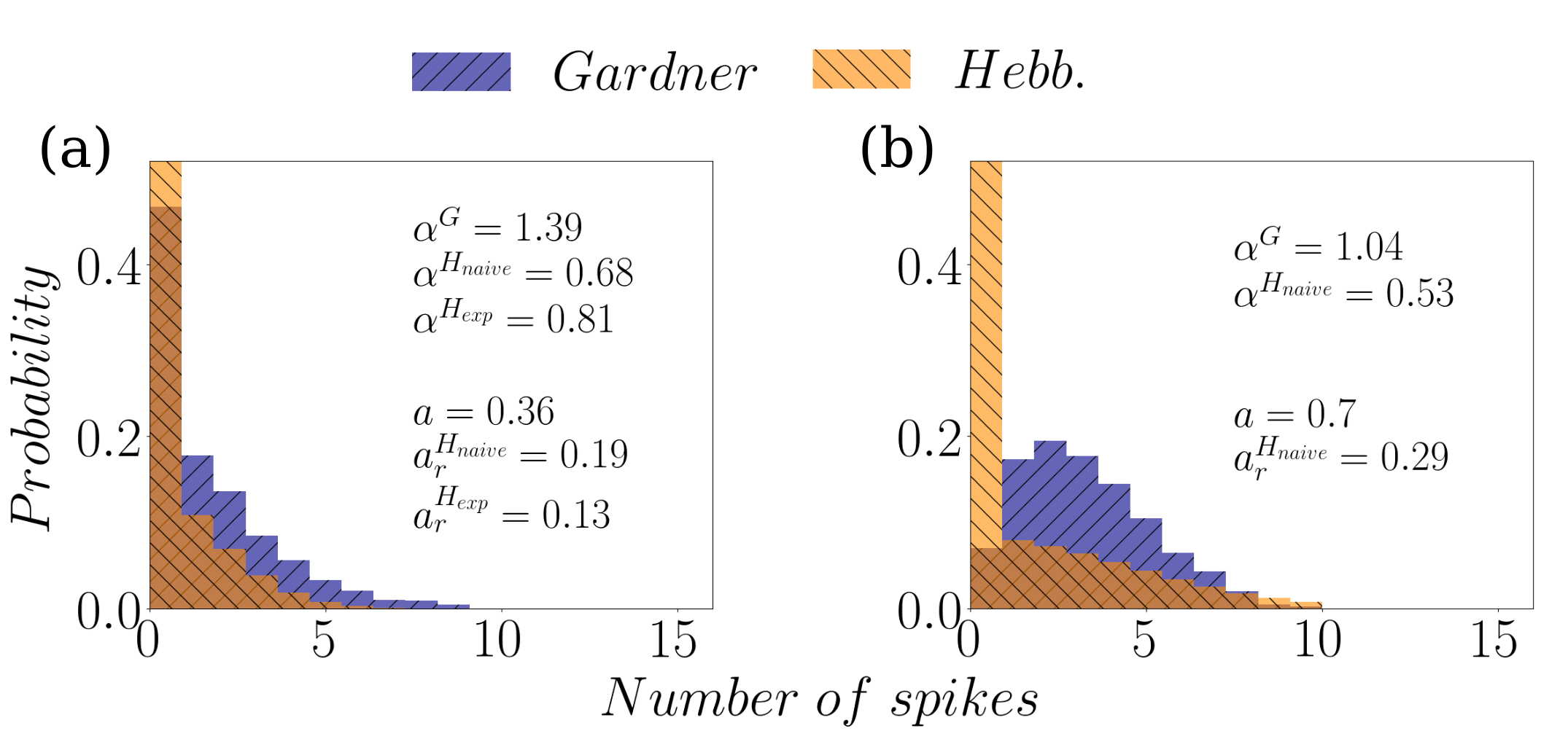
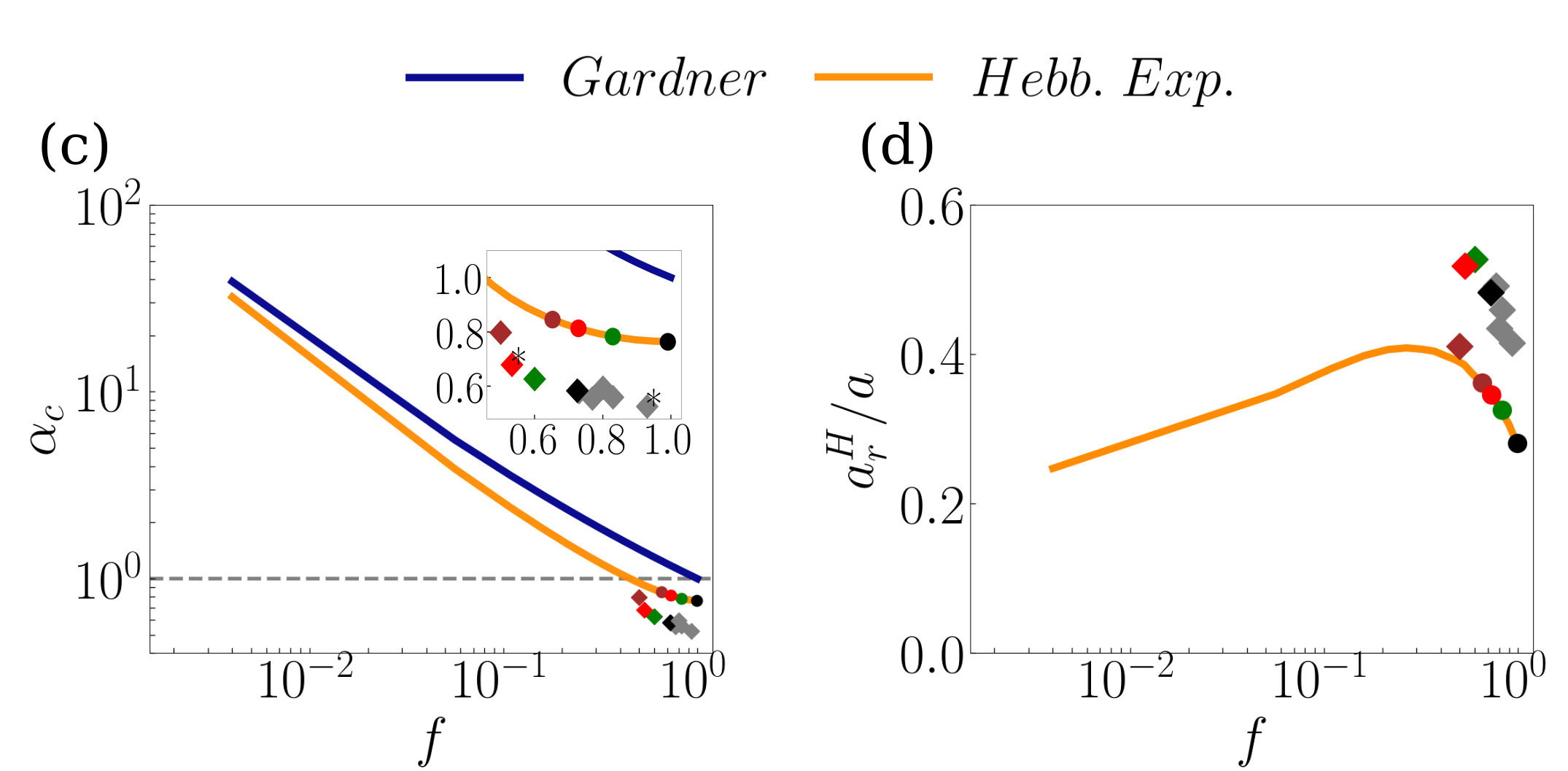
Figure 3: Hebbian vs. Gardner capacity for experimental data. (a,b) histograms of two experimentally recorded spike counts (blue) and the retrieved distributions, if the patterns were stored using Hebbian learning (orange). Note that the retrieved distributions à la Gardner would be the same as the stored patterns. (c) Analytically calculated Gardner capacity $\alpha_{c}^{G}$ (blue), compared to $\alpha_{c}^{H_{e}xp}$ for the Hebbian learning of an exponential distribution (orange, circles). $\alpha_{c}^{H_{naive}}$ is shown by diamonds. The asterisks mark the two cells whose distribution is plotted in (a-b). (d) Sparsification of the retrieved patterns, for Hebbian learning.

VI Discussion

–. While instrumental in conceptualizing memory storage Amit and Brunel (1997); *Bat+98; *Yoo+13, Hebbian learning has been widely considered a poor man’s option, relative to more powerful machine learning algorithms that could reach the Gardner bound for binary units and patterns. No binary or quasibinary pattern of activity has ever been observed in the cerebral cortex, however. A few studies have considered TL units, showing them to be less susceptible to memory mix-up effects Treves (1991b); *Rou+03 or perturbations in the weights and inputs values Baldassi et al. (2019) but, in the framework of à la Gardner calculations, they have focused on issues other than associative networks storing sparse representations. For instance, a replica analysis was carried out in Bollé et al. (1993) with a generic gain function, but then discussed only in a quasibinary regime. Others considered monotonically increasing activation functions under the constraint of nonnegative weights Clopath and Brunel (2013). Here, we report the analytical derivation of the Gardner capacity for TL networks, validate it via perceptron training, and compare it with Hebbian learning. We find that the bound can be reached or even surpassed, and that retrieval leads to sparsification. For sample experimental distributions, we find that one-shot Hebbian learning can utilize $50-80\%$ of the available “errorless” capacity if retrieving sparser activity, compatible with recent observations Lim et al. (2015).

In deriving the Gardner bound, we assumed errorless retrieval and it remains to be seen how much allowing errors increases this bound for TL units and neurally plausible distributions. For the binary case of Gardner et al. (1989), as already mentioned, this errorless bound is still above the Hebbian capacity of the highly diluted regime, with its continuous (second order) transition, i.e., with vanishing overlap at storage capacity Gardner et al. (1989). How does the overlap behave in the TL case? For highly diluted TL networks with Hebbian learning, in fact, except for special cases, the transition at capacity is discontinuous: the overlap drops to zero from a non-zero value that depends on the distribution of stored neural activity but can be small Schönsberg et al. (ming). It is worth noting, though, that while in the binary case the natural measure of error is simply the fraction of units misaligned at retrieval, in the TL case error can be quantified in other ways. In the extreme in which only the most active cells remain active at retrieval, those retrieved memories cannot be regarded as the full pattern, with its entire information content, but more as a pointer, effective perhaps as a mechanism only to distinguish between different possible patterns or to address the full memory elsewhere, as posited in index theories of 2-stage memory retrieval Teyler and DiScenna (1986). Further understanding would also derive from comparing the maximal information content per synapse for TL units, with Hebbian or iterative learning, as previously studied for binary networks Nadal and Toulouse (1990). Using nonbinary patterns might also afford a solution to the low storage capacity observed in balanced memory networks storing binary patterns Roudi and Latham (2007).

Our focus here has been on memory storage in associative neural networks, with the overarching conclusion that the relative efficiency of Hebbian learning is much higher when units have a similar transfer function to real cortical neurons. The efficiency of local learning rules had also been challenged by their comparatively weaker performance in other (machine learning) settings Bartunov et al. (2018), while results to the contrary are also reported Amit (2019); Krotov and Hopfield (2019). It may therefore be argued that the efficiency of local learning in these settings might also be fundamentally dependent on both the types of units used and the data, observations consistent with the findings in Krotov and Hopfield (2019) and Bartunov et al. (2018), respectively. In evaluating a learning rule, it may therefore be crucial to consider whether it is suited to the transfer function and data representation it operates on.

References

- Brown et al. (1990) T. H. Brown, E. W. Kairiss, and C. L. Keenan, Annual review of neuroscience 13, 475 (1990).
- Hebb (1949) D. O. Hebb, The Organization of Behavior: a Neuropsychological Theory (J. Wiley; Chapman & Hall, 1949).
- Amit (1992) D. J. Amit, Modeling Brain Function: The World of Attractor Neural Networks (Cambridge university press, 1992).
- Hopfield (1982) J. J. Hopfield, Proceedings of the national academy of sciences 79, 2554 (1982).
- Amit et al. (1987) D. J. Amit, H. Gutfreund, and H. Sompolinsky, Annals of physics 173, 30 (1987).
- Derrida et al. (1987) B. Derrida, E. Gardner, and A. Zippelius, EPL (Europhysics Letters) 4, 167 (1987).
- Gardner (1988) E. Gardner, Journal of physics A: Mathematical and general 21, 257 (1988).
- Hartline and Ratliff (1957) H. K. Hartline and F. Ratliff, The Journal of general physiology 40, 357 (1957).
- Hartline and Ratliff (1958) H. K. Hartline and F. Ratliff, The Journal of general physiology 41, 1049 (1958).
- Treves (1990a) A. Treves, Journal of Physics A: Mathematical and General 23, 2631 (1990a).
- Nair and Hinton (2010) V. Nair and G. E. Hinton, in Proceedings of the 27th international conference on machine learning (ICML-10) (2010) pp. 807–814.
- Maas et al. (2013) A. L. Maas, A. Y. Hannun, and A. Y. Ng, in Proc. icml, 1 (2013) p. 3.
- He et al. (2015) K. He, X. Zhang, S. Ren, and J. Sun, in Proceedings of the IEEE international conference on computer vision (2015) pp. 1026–1034.
- Goodfellow et al. (2016) I. Goodfellow, Y. Bengio, and A. Courville, Deep learning (MIT press, 2016).
- Pereira and Brunel (2018) U. Pereira and N. Brunel, Neuron 99, 227 (2018).
- Gardner et al. (1989) E. Gardner, S. Mertens, and A. Zippelius, Journal of Physics A: Mathematical and General 22, 2009 (1989).
- Tsodyks and Feigel’man (1988) M. V. Tsodyks and M. V. Feigel’man, EPL (Europhysics Letters) 6, 101 (1988).
- Bollé et al. (1993) D. Bollé, R. Kuhn, and J. Van Mourik, Journal of Physics A: Mathematical and General 26, 3149 (1993).
- Treves et al. (1999) A. Treves, S. Panzeri, E. T. Rolls, M. Booth, and E. A. Wakeman, Neural Computation 11, 601 (1999).
- Treves (1991a) A. Treves, Journal of Physics A: Mathematical and General 24, 327 (1991a).
- Treves and Rolls (1991) A. Treves and E. T. Rolls, Network: Computation in Neural Systems 2, 371 (1991).
- Treves (1990b) A. Treves, Physical Review A 42, 2418 (1990b).
- Roudi and Treves (2006) Y. Roudi and A. Treves, Physical Review E 73, 061904 (2006).
- Fuster and Jervey (1981) J. M. Fuster and J. P. Jervey, Science 212, 952 (1981).
- Miyashita (1988) Y. Miyashita, Nature 335, 817 (1988).
- Nakamura and Kubota (1995) K. Nakamura and K. Kubota, Journal of neurophysiology 74, 162 (1995).
- Amit et al. (1997) D. J. Amit, S. Fusi, and V. Yakovlev, Neural computation 9, 1071 (1997).
- Rolls and Treves (1998) E. T. Rolls and A. Treves, Neural Networks and Brain Function (Oxford university press, Oxford, 1998).
- Lim et al. (2015) S. Lim, J. L. McKee, L. Woloszyn, Y. Amit, D. J. Freedman, D. L. Sheinberg, and N. Brunel, Nature neuroscience 18, 1804 (2015).
- Buzsáki and Mizuseki (2014) G. Buzsáki and K. Mizuseki, Nature Reviews Neuroscience 15, 264 (2014).
- Amit and Brunel (1997) D. J. Amit and N. Brunel, Network: Computation in Neural Systems 8, 373 (1997).
- Battaglia and Treves (1998) F. P. Battaglia and A. Treves, Neural Computation 10, 431 (1998).
- Yoon et al. (2013) K. Yoon, M. A. Buice, C. Barry, R. Hayman, N. Burgess, and I. R. Fiete, Nature neuroscience 16, 1077 (2013).
- Treves (1991b) A. Treves, Journal of Physics A: Mathematical and General 24, 2645 (1991b).
- Roudi and Treves (2003) Y. Roudi and A. Treves, Physical Review E 67, 041906 (2003).
- Baldassi et al. (2019) C. Baldassi, E. M. Malatesta, and R. Zecchina, Physical review letters 123, 170602 (2019).
- Clopath and Brunel (2013) C. Clopath and N. Brunel, PLoS computational biology 9 (2013).
- Schönsberg et al. (ming) F. Schönsberg, Y. Roudi, and A. Treves, (forthcoming).
- Teyler and DiScenna (1986) T. J. Teyler and P. DiScenna, Behavioral neuroscience 100, 147 (1986).
- Nadal and Toulouse (1990) J.-P. Nadal and G. Toulouse, Network: Computation in Neural Systems 1, 61 (1990).
- Roudi and Latham (2007) Y. Roudi and P. E. Latham, PLoS Comput Biol 3, e141 (2007).
- Bartunov et al. (2018) S. Bartunov, A. Santoro, B. Richards, L. Marris, G. E. Hinton, and T. Lillicrap, in Advances in Neural Information Processing Systems 31, edited by S. Bengio, H. Wallach, H. Larochelle, K. Grauman, N. Cesa-Bianchi, and R. Garnett (Curran Associates, Inc., 2018) pp. 9368–9378.
- Amit (2019) Y. Amit, Frontiers in computational neuroscience 13, 18 (2019).
- Krotov and Hopfield (2019) D. Krotov and J. J. Hopfield, Proceedings of the National Academy of Sciences 116, 7723 (2019).