Combined Sparse Regularization
for Nonlinear Adaptive Filters

Abstract

Nonlinear adaptive filters often show some sparse behavior due to the fact that not all the coefficients are equally useful for the modeling of any nonlinearity. Recently, a class of proportionate algorithms has been proposed for nonlinear filters to leverage sparsity of their coefficients. However, the choice of the norm penalty of the cost function may be not always appropriate depending on the problem. In this paper, we introduce an adaptive combined scheme based on a block-based approach involving two nonlinear filters with different regularization that allows to achieve always superior performance than individual rules. The proposed method is assessed in nonlinear system identification problems, showing its effectiveness in taking advantage of the online combined regularization.

I Introduction

Very often, in estimating an impulse response that characterizes an unknown system, we may notice some kind of sparsity. Such sparse behavior of the system response is often due to the fact that most of its energy is contained in a small part of it [1]. This means that a small part of the impulse response is characterized by large magnitude coefficients, while the rest shows negligible values. In system identification problems, this behavior can be exploited to improve the overall modeling performance by introducing a regularizing penalty in the cost function. In this sense, sparse regularization is widely employed in several fields of application, highlighting recently some examples found in underwater communication [2], compressive sensing [3], Alzheimer’s disease diagnosis [4], wireless communications [5], adaptive beamforming [6, 7] and large-scale classification [8], among others.

Sparsity may characterize not only linear systems but also nonlinear ones. In nonlinear modeling problems, which can be found in several real-world applications [9], nonlinear expansions or transformation may introduce a large number of coefficients, some of which can result to be useless for the purpose of nonlinear modeling. This often leads to overfitting phenomena and performance degradation [10]. In order to tackle this problem and avoid any deterioration in performance, we may think to involve any methodology capable of selecting only the most significant nonlinear elements, i.e., those providing the best modeling performance. However, in real-world problems that require an online estimation, this kind of selection process is often not so trivial to be implemented. In particular, when a nonlinearity is nonstationary or depending on a time-varying signal, it is not possible to select a priori the most significant nonlinear coefficients. In linear-in-the-parameters (LIP) nonlinear filters, one of the most effective approach to avoid overfitting is represented by adaptive algorithms involving sparse regularization [11]. In the last years, several sparse nonlinear algorithms have been proposed, including kernel-based methods [12, 13] and polynomial methods [14], among others.

In this paper we focus on the class of LIP nonlinear filters known as functional link adaptive filters (FLAFs) [11, 15, 10, 16]. Functional link models are widespread in the literature due to their flexibility and the large range of application in which they can be used [17, 18, 19, 20]. They are basically characterized by a nonlinear transformation of the input by any nonlinear series expansion. Depending on the problem and on the nonlinearity to model, the number of functional links may be rather high, thus causing sparsity in the FLAF coefficient vector. However, this behavior can be exploited by imposing any sparsity constraint in the minimization problem. In that sense, proportionate regularization has been mainly considered to develop proportionate FLAFs (PFLAFs) achieving promising results [11, 10]. However, the possibility of using an $\ell_{1}$-norm constraint besides the classic proportionality can also be advantageous due to its desirable properties of inducing sparsity while keeping the convexity of the cost function [21, 22]. One of the most successfully used class of online adaptive algorithms showing an $\ell_{1}$ relaxation is based on zero-attracting proportionate adaptation [23, 24, 25].

In order to take always advantage of different sparse regularization rules, we propose the use of a combined nonlinear filtering scheme that permits to improve modeling performance when the a priori knowledge about the nonlinearity to be modeled is limited [26, 27]. In particular, the proposed scheme involves an adaptive convex combination of two PFLAFs, involving one with a $\ell_{1}$-norm constraint. Moreover, we employ a block-based strategy that takes into account the cyclic nature of sparse functional links[10].

The paper is organized as follows. Section II briefly reviews the sparse functional link modeling, while two different sparse regularization rules are introduced in Section III. In Section IV, we introduce the block-based combination scheme for the sparse FLAFs, and in Section V experimental results are shown. Concluding remarks are drawn in Section VI.

II Nonlinear Modeling with Sparse FLAF

II-A A Review of the Functional Link Adaptive Filter

The functional link adaptive filter (FLAF) [18] is a LIP nonlinear filter that expands a linear input signal ${\mathbf{x}}_{\mbox{\tiny${\rm{L}}$},n}\in\mathbb{R}^{M}=\left[{\begin{array}[]{*{20}c}{x\left[n\right]}&{x\left[n-1\right]}&\ldots&{x\left[n-M+1\right]}\\ \end{array}}\right]^{\text{T}}$, being $M$ the length of the regression vector, in order to filter it in a higher dimensional space. The transformation of the input signal is performed by applying a nonlinear expansion series in order to produce the nonlinear signal. The chosen functions of the expansion series represent the set of functional links $\Phi=\left\{\mbox{\large$\varphi$}_{\scriptscriptstyle 0}\left(\cdot\right),\ldots,\mbox{\large$\varphi$}_{\scriptscriptstyle Q_{\mbox{\tiny${\rm{f}}$}}-1}\left(\cdot\right)\right\}$, where $Q_{\mbox{\tiny${\rm{f}}$}}$ is the number of the chosen functional links. One of the most popular choice for populating the functional link set is to use the trigonometric series expansion, which can be described as:

$$\mbox{\large$\varphi$}_{\scriptscriptstyle j}\left(x\left[n-i\right]\right)=\left\{{\begin{array}[]{*{20}c}{\sin\left({p\pi x\left[{n-i}\right]}\right),\hfill}&{j=2p-2\hfill}\\ {\cos\left({p\pi x\left[{n-i}\right]}\right),\hfill}&{j=2p-1\hfill}\\ \end{array}}\right.$$ (1)

for $i=0,\ldots,M-1$. In (1), $p=1,\ldots,P$ is the expansion index, where $P$ is the expansion order, and $j=0,\ldots,Q_{\mbox{\tiny${\rm{f}}$}}-1$ is the functional link index. For the trigonometric memoryless expansion, the overall number of functional links contained in the set $\Phi$ is equal to $Q_{\mbox{\tiny${\rm{f}}$}}=2P$.

The overall expanded vector resulting from the application of the functional link set to the input signal is denoted as $\mathbf{g}_{n}\in\mathbb{R}^{M_{\mbox{\tiny${\rm{e}}$}}}=\left[\begin{array}[]{*{20}c}{g_{0}\left[n\right]}&{g_{1}\left[n\right]}&\ldots&{g_{M_{\mbox{\tiny${\rm{e}}$}}-1}\left[n\right]}\end{array}\right]^{\text{T}}$, where $M_{\mbox{\tiny${\rm{e}}$}}\geq M$ is the length of the expanded vector. Then, the signal $\mathbf{g}_{n}$, which represents the input in a higher dimensional space, can be processed by any adaptive filter to achieve the system output.

The functional link set $\Phi$ may contain both linear and nonlinear functions. However, we assume that all the functional links are nonlinear [18], such that the resulting expanded vector $\mathbf{g}_{n}$ is completely composed of nonlinear elements. This allows to increase the flexibility of the adaptive scheme in those problems which require the modeling of linear and nonlinear components, since we can devote one adaptive filter $\mathbf{w}_{\mbox{\tiny${\rm{L}}$},n}\in\mathbb{R}^{M}=\left[{{\begin{array}[]{*{20}c}{w_{\mbox{\tiny${\rm{L}}$},0}\left[n\right]}&\ldots\\ \end{array}}}\right.$ $\left.{{\begin{array}[]{*{20}c}{w_{\mbox{\tiny${\rm{L}}$},M-1}\left[{n}\right]}\\ \end{array}}}\right]^{\text{T}}$ for the non-expanded linear input ${\mathbf{x}}_{\mbox{\tiny${\rm{L}}$},n}$ and another adaptive filter $\mathbf{w}_{\mbox{\tiny${\rm{FL}}$},n}\in\mathbb{R}^{M_{\mbox{\tiny${\rm{e}}$}}}=\left[{{\begin{array}[]{*{20}c}{w_{\mbox{\tiny${\rm{FL}}$},0}\left[n\right]}&\ldots\\ \end{array}}}\right.$ $\left.{{\begin{array}[]{*{20}c}{w_{\mbox{\tiny${\rm{FL}}$},M_{\mbox{\tiny${\rm{e}}$}}-1}\left[{n}\right]}\\ \end{array}}}\right]^{\text{T}}$ for $\mathbf{g}_{n}$, enabling us to choose different learning algorithms with different capabilities for each adaptive filter. This method is detailed in [18].

II-B Sparsity in FLAF

The concept of sparsity in a linear filter has been dealt with quite extensively in the literature. However, a major attention is required for a LIP nonlinear filter, as in the case of $\mathbf{w}_{\mbox{\tiny${\rm{FL}}$},n}$.

In order to understand how sparsity behaviors occur in FLAFs, it is sufficient to analyze the energy of the coefficient vector $\mathbf{w}_{\mbox{\tiny${\rm{FL}}$},n}$ at steady state [10], i.e., for $n\to\infty$. As a result, the early functional links of the set $\Phi$, which have small values of the expansion order (i.e., $p$ close to $1$), generate the most significant nonlinear elements for the purpose of the nonlinear modeling. On the other hand, the remaining functional links of $\Phi$ produce only minor, or even negligible, variations in the modeling results. This is physically motivated by the fact that high-order functional links (i.e., with $p\to P$) aim at modeling those nonlinear components that not always appear in a nonlinear distortion (e.g., high-order harmonics), thus resulting in a slight improvement that might not always occur. In terms of energy, it is possible to describe the sparsity behavior in functional links as an exponential decay from early to late elements, in which the larger the expansion order the longer the tail. Such behavior occurs for each input sample that is expanded by the functional link set $\Phi$, therefore, overall, we may have a periodic sparse behavior for $\mathbf{w}_{\mbox{\tiny${\rm{FL}}$},\infty}$ [10].

III Sparse Functional Link Adaptive Filters

In this section, we derive two sparse FLAFs, $\mathbf{w}_{\mbox{\tiny${\rm{FL}}$}1,n}$ and $\mathbf{w}_{\mbox{\tiny${\rm{FL}}$}2,n}$, respectively using an $\ell_{1}$-norm proportionate and a classic proportionate regularization.

III-A Derivation of the $\ell_{1}$-Regularized PFLAF

In order to derive the optimization algorithms for the $\ell_{1}$ sparse functional links, we can express the $\ell_{1}$-constrained optimization problem, considering the least-perturbation property and the natural gradient adaptation, as suggested in [11], thus:

$$\arg\mathop{\min}\limits_{\mathbf{w}_{\mbox{\tiny${\rm{FL}}$}1,n}}\left\|\mathbf{w}_{\mbox{\tiny${\rm{FL}}$}1,n}-\mathbf{w}_{\mbox{\tiny${\rm{FL}}$}1,n-1}\right\|_{\mathbf{Q}_{1,n}^{-1}}^{2}+\gamma\left\|\mathbf{Q}_{1,n}^{-1}\mathbf{w}_{\mbox{\tiny${\rm{FL}}$}1,n}\right\|_{1}$$ (2)

$$\text{s.t.}\ \ \ \varepsilon_{1}\left[n\right]=0$$

where $\mathbf{Q}_{1,n}^{-1}$ is a distance correction matrix with respect to the Euclidean metric, $\gamma$ is a very small constant and the constraint $\varepsilon_{1}\left[n\right]=0$ can be derived from the a posteriori output estimation error signal $\varepsilon_{1}\left[n\right]=d\left[n\right]-\mathbf{x}_{\mbox{\tiny${\rm{L}}$},n}^{\text{T}}\mathbf{w}_{\mbox{\tiny${\rm{L}}$},n}-\mathbf{g}_{n}^{\text{T}}\mathbf{w}_{\mbox{\tiny${\rm{FL}}$}1,n}$. The problem in (2) involves an $\ell_{1}$-norm penalty term that aims at scaling the coefficient vector $\mathbf{w}_{\mbox{\tiny${\rm{FL}}$}1,n}$ by the distance correction matrix $\mathbf{Q}_{1,n}^{-1}$ and thus regularizing the solution by mainly exploiting inactive coefficients.

The solution to the problem (2), with respect to $\mathbf{w}_{\mbox{\tiny${\rm{FL}}$}1,n}$, can be expressed as:

$$\begin{split}\mathbf{w}_{\mbox{\tiny${\rm{FL}}$}1,n}&=\mathbf{w}_{\mbox{\tiny${\rm{FL}}$}1,n-1}+\mu_{\mbox{\tiny${\rm{FL}}$}}\frac{\mathbf{Q}_{1,n}\mathbf{g}_{n}e_{\mbox{\tiny${\rm{FL}}$}1}\left[n\right]}{\mathbf{g}_{n}^{\text{T}}\mathbf{Q}_{1,n}\mathbf{g}_{n}+\delta}\\ &-\gamma_{\mbox{\tiny${\rm{R}}$}}\left[n\right]\frac{\operatorname{sgn}\left(\mathbf{w}_{\mbox{\tiny${\rm{FL}}$}1,n-1}\right)}{1+\epsilon\left|\mathbf{w}_{\mbox{\tiny${\rm{FL}}$}1,n-1}\right|},\end{split}$$ (3)

where $e_{\mbox{\tiny${\rm{FL}}$}1}\left[n\right]=d\left[n\right]-\mathbf{x}_{\mbox{\tiny${\rm{L}}$},n}^{\text{T}}\mathbf{w}_{\mbox{\tiny${\rm{L}}$},n-1}-\mathbf{g}_{n}^{\text{T}}\mathbf{w}_{\mbox{\tiny${\rm{FL}}$}1,n-1}=d\left[n\right]-y_{\mbox{\tiny${\rm{L}}$}}\left[n\right]-y_{\mbox{\tiny${\rm{FL}}$}1}\left[n\right]$, $\delta$ is a regularization factor, $\mu_{\mbox{\tiny${\rm{FL}}$}1}$ is a step-size parameter, and $\operatorname{sgn}\left(\cdot\right)$ is intended as an element-wise sign function defined for the $i$-th entry of $\mathbf{w}_{\mbox{\tiny${\rm{FL}}$}1,n}$ as:

$$\operatorname{sgn}\left({w_{\mbox{\tiny${\rm{FL}}$}1,i}\left[n\right]}\right)=\left\{{\begin{array}[]{*{20}c}{{{w_{\mbox{\tiny${\rm{FL}}$}1,i}\left[n\right]}\mathord{\left/{\vphantom{{w_{\mbox{\tiny${\rm{FL}}$}1,i}\left[n\right]}{\left|{w_{\mbox{\tiny${\rm{FL}}$}1,i}\left[n\right]}\right|,}}}\right.\kern-1.2pt}{\left|{w_{\mbox{\tiny${\rm{FL}}$}1,i}\left[n\right]}\right|,}}}&{w_{\mbox{\tiny${\rm{FL}}$}1,i}\left[n\right]\neq 0}\\ {0,}&{w_{\mbox{\tiny${\rm{FL}}$}1,i}\left[n\right]=0}\\ \end{array}}\right.$$ (4)

Equation (3) involves some considerations. First, we assumed that most of the weights do not change their sign at each iteration, especially those weights that are inactive, i.e, that are close to zero at steady state. Therefore, the term $\operatorname{sgn}\left(\mathbf{w}_{\mbox{\tiny${\rm{FL}}$}1,n}\right)$, which contains the unknown new update, can be approximated by $\operatorname{sgn}\left(\mathbf{w}_{\mbox{\tiny${\rm{FL}}$}1,n-1}\right)$ without affecting the convergence behavior [23, 25].

Moreover, with respect to original PFLAFs [16, 10], the FLAF based on the $\ell_{1}$ penalty involves a third additional term, the “zero attractor”, which shrinks the inactive weights of $\mathbf{w}_{\mbox{\tiny${\rm{FL}}$}1,n-1}$ to zero. However, such term may lose its effectiveness as the sparsity of a system decreases, i.e., the number of active coefficients increases. To overcome this limitations, the $\ell_{1}$ regularization term $\left\|\mathbf{Q}_{1,n}^{-1}\mathbf{w}_{n}\right\|_{1}$ in (2) has been replaced by a log-sum penalty term $\left\|\mathbf{Q}_{1,n}^{-1}\log\left(1+\epsilon\mathbf{w}_{\mbox{\tiny${\rm{FL}}$}1,n}\right)\right\|_{1}$, where $\epsilon$ is a small constant [28, 23].

Finally, in (3), $\gamma_{\mbox{\tiny${\rm{R}}$}}\left[n\right]=\epsilon\gamma\mu_{\mbox{\tiny${\rm{R}}$}}\left[n\right]$, where $\mu_{\mbox{\tiny${\rm{R}}$}}\left[n\right]$ is a nonparametric variable step size (VSS) [29, 22], defined as:

$$\mu_{\mbox{\tiny${\rm{R}}$}}\left[n\right]=\left|1-\frac{\sqrt{\left|\widehat{\sigma}_{d}^{2}\left[n\right]-\widehat{\sigma}_{y_{\mbox{\tiny${\rm{L}}$}}}^{2}\left[n\right]-\widehat{\sigma}_{y_{\mbox{\tiny${\rm{FL}}$}1}}^{2}\left[n\right]\right|}}{\widehat{\sigma}_{e_{\mbox{\tiny${\rm{FL}}$}1}}^{2}\left[n\right]+\xi}\right|.$$ (5)

In (5), the general parameter $\widehat{\sigma}_{\theta}^{2}\left[n\right]$ represents the power estimate of the sequence $\theta\left[n\right]$, being $\theta=\left\{d,y,e\right\}$, and it can be computed as $\widehat{\sigma}_{\theta}^{2}\left[n\right]=\beta\widehat{\sigma}_{\theta}^{2}\left[n-1\right]+\left(1-\beta\right)\theta^{2}\left[n\right]$ where $\beta\to 1$ is a forgetting factor. $\xi$ is a small positive constant that avoids divisions by zero.

The update equation (3) defines the VSS reweighted zero attractor FLAF. The last term of (3), in which the division is performed element-wise, is the reweighted zero attractor, whose aim is to shrink to zero those coefficients whose magnitude is comparable to $1/\epsilon$, thus preserving the most active coefficients. This usually results in an improvement in terms of convergence rate and steady state performance.

III-B Derivation of the Proportionate FLAF

The second sparse FLAF can be derived by formalizing the following optimization problem:

$$\arg\mathop{\min}\limits_{\mathbf{w}_{\mbox{\tiny${\rm{FL}}$}2,n}}\left\|\mathbf{w}_{\mbox{\tiny${\rm{FL}}$}2,n}-\mathbf{w}_{\mbox{\tiny${\rm{FL}}$}2,n-1}\right\|_{\mathbf{Q}_{2,n}^{-1}}^{2}$$ (6)

$$\text{s.t.}\ \varepsilon_{2}\left[n\right]= \left(1-\frac{\mu_{\mbox{\tiny${\rm{L}}$}}\left\|\mathbf{x}_{\mbox{\tiny${\rm{L}}$},n}\right\|_{2}^{2}}{\left\|\mathbf{x}_{\mbox{\tiny${\rm{L}}$},n}\right\|_{2}^{2}+\delta_{\mbox{\tiny${\rm{L}}$}}}-\frac{\mu_{\mbox{\tiny${\rm{FL}}$}2}\left\|\mathbf{g}_{n}\right\|_{\mathbf{Q}_{2,n}}^{2}}{\left\|\mathbf{g}_{n}\right\|_{\mathbf{Q}_{2,n}}^{2}+\delta_{\text{\tiny{PFL}}}}\right)e_{\mbox{\tiny${\rm{FL}}$}2}\left[n\right]$$

where $\mu_{\mbox{\tiny${\rm{L}}$}}$ and $\mu_{\mbox{\tiny${\rm{FL}}$}2}$ are step-size parameters, $\delta_{\mbox{\tiny${\rm{L}}$}}$ and $\delta_{\text{\tiny{PFL}}2}$ are regularization factors. The resulting solution, whose complete derivation can be found in [11], can be written as:

$$\mathbf{w}_{\mbox{\tiny${\rm{FL}}$}2,n}=\mathbf{w}_{\mbox{\tiny${\rm{FL}}$}2,n-1}+\mu_{\mbox{\tiny${\rm{FL}}$}2}\frac{\mathbf{Q}_{2,n}\mathbf{g}_{n}}{\mathbf{g}_{n}{{}^{\text{T}}}\mathbf{Q}_{2,n}\mathbf{g}_{n}+\delta_{\text{\tiny{PFL}}}}e_{\mbox{\tiny${\rm{FL}}$}2}\left[n\right].$$ (7)

III-C Choice of the weighting matrix

The matrix $\mathbf{Q}_{j,}n$, with $j=1,2$, in (3) and (7), also known as proportionate matrix, aims at weighting the coefficients of $\mathbf{w}_{\mbox{\tiny${\rm{FL}}$}j,n}$ proportionally to the contribution they provide to the modeling. $\mathbf{Q}_{j,n}$ can be chosen as a diagonal matrix $\mathbf{Q}_{j,n}\in\mathbb{R}^{M_{\mbox{\tiny${\rm{e}}$}}}={\text{diag}}\left\{{\begin{array}[]{*{20}c}{q_{j,0}\left[n\right]}&\ldots&{q_{j,M_{\mbox{\tiny${\rm{e}}$}}-1}\left[n\right]}\\ \end{array}}\right\}$, whose diagonal elements are derived according to the coefficients at the time instant $n-1$.

Several choices can be made for deriving the diagonal elements of $\mathbf{Q}_{j,n}$. We choose the same derivation for both the sparse FLAFs according to [30, 11]:

$$q_{j,k}\left[n\right]=\frac{1-\alpha}{2M_{\mbox{\tiny${\rm{e}}$}}}+\left(1+\alpha\right)\frac{\left|w_{\mbox{\tiny${\rm{FL}}$}j,k}\left[n-1\right]\right|}{\xi+2\sum_{i=a}^{b}w_{\mbox{\tiny${\rm{FL}}$}j,k\left[n-1\right]},}$$ (8)

with $k=0,\ldots,M_{\mbox{\tiny${\rm{e}}$}}-1$ and $\xi$ being a small positive value. In (8), the proportionality factor $-1\leq\alpha\leq 1$ assumes a value close to $1$ when a high degree of sparseness is expected, while, on the contrary, a low degree is expected when the proportionality factors are close to $-1$.

IV Combined Sparse Regularization Scheme

In order to take advantage of the two sparse FLAFs, we adopt an adaptive combined architecture characterized by a linear branch and, in parallel, a convex combination of the FLAFs, as represented in Fig. 1.

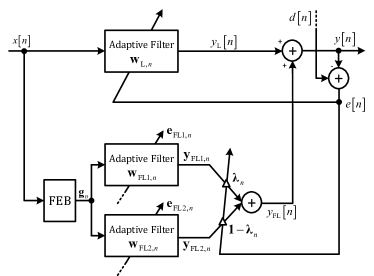
Figure 1: The proposed combined scheme where the filter block outputs are combined by the mixing parameter vectors.

The output of the linear branch is performed as a classic linear filtering, while the nonlinear branch involves the generation of the expanded signal $\mathbf{g}_{n}$, as previously described, which is then fed into both the adaptive filters, thus generating the individual outputs and errors, $y_{\mbox{\tiny${\rm{FL}}$}j}\left[n\right]=\mathbf{g}_{n}^{\text{T}}\mathbf{w}_{\mbox{\tiny${\rm{FL}}$}j,n-1}$ for $j=1,2$. The overall output of the nonlinear branch is achieved by combining convexly the individual filter outputs in a block-based fashion, as described in [10].

The block-based combination takes advantage of the periodic nature of the sparse energy behavior of functional links, as detailed in [10]. Each group of expanded samples may be characterized by a similar energy decay to that of the adjacent groups. Based on this property, we may think to divide the coefficient vectors $\mathbf{w}_{\mbox{\tiny${\rm{FL}}$}1,n}$ and $\mathbf{w}_{\mbox{\tiny${\rm{FL}}$}2,n}$ into $L$ blocks, each one consisting of $M_{\text{b}}=Q_{\mbox{\tiny${\rm{f}}$}}/L$ coefficients. Therefore, the output of the block-based combination can be written as:

$$\begin{split}y_{\mbox{\tiny${\rm{FL}}$}}\left[n\right]&=\sum_{i=0}^{M-1}\left(\sum_{l=1}^{L}\lambda_{l}\left[n\right]\mathbf{g}_{n}^{\left(iL+l\right){\text{T}}}\mathbf{w}_{\mbox{\tiny${\rm{FL}}$}1,n-1}^{\left(iL+l\right)}\right.\\ &+\left.\left(1-\lambda_{l}\left[n\right]\right)\mathbf{g}_{n}^{\left(iL+l\right){\text{T}}}\mathbf{w}_{\mbox{\tiny${\rm{FL}}$}2,n-1}^{\left(iL+l\right)}\right)\end{split}$$ (9)

where the index $i$ denotes the input signal sample that is expanded by (1), $l$ represents the block index and $\lambda_{l}\left[n\right]$ is the mixing parameter associated to the $l$-th block. The $l$-th adaptive mixing parameter $\lambda_{l}\left[n\right]$, with $l=1,\ldots,L$, in (9) balances the combination between the $l$-th blocks of the two filters $\mathbf{w}_{\mbox{\tiny${\rm{FL}}$}j}\left[n\right]$ ($j=1,2$), giving more importance to the best performing filter block [26]. Such awareness is obtained according to a mean-square error minimization. In particular, the adaptation of $\lambda_{l}\left[n\right]$ is performed by using an auxiliary adaptive parameter for each block $a_{l}\left[n\right]$, which is related to $\lambda_{l}\left[n\right]$ by means of a sigmoid function that keeps the mixing parameter in the range $\left[0,1\right]$ [26, 27]:

$$\lambda_{l}\left[n\right]=\eta\left(\frac{1}{1+e^{-a_{l}\left[n\right]}}-\theta\right),$$ (10)

where $\theta=1/\left(1+e^{4}\right)$ and $\eta=1/\left(1-2\theta\right)$. The update rule for the auxiliary parameter for the $l$-th block is:

$$\begin{split}a_{l}\left[n\right]=&a_{l}\left[n-1\right]+\frac{\mu_{\text{c}}}{\eta r_{l}\left[n-1\right]}e\left[n\right]\Delta y_{\mbox{\tiny${\rm{FL}}$},l}\left[n\right]\\ &\cdot\left(\lambda_{l}\left[n\right]+\theta\eta\right)\left(\eta-\theta\eta-\lambda_{l}\left[n\right]\right)\end{split}$$ (11)

for $l=1,\ldots,L$, where

$$\Delta y_{\mbox{\tiny${\rm{FL}}$},l}\left[n\right]=\sum_{i=1}^{M}\mathbf{g}_{n}^{\left(i,l\right){\text{T}}}\left(\mathbf{w}_{\mbox{\tiny${\rm{FL}}$}1,n-1}^{\left(i,l\right)}-\mathbf{w}_{\mbox{\tiny${\rm{FL}}$}2,n-1}^{\left(i,l\right)}\right),$$ (12)

where the superscript $\left(i,l\right)$ denotes the $l$-th block related to the $i$-th entry. In (11), $\mu_{\text{c}}$ is the step-size parameter of the adaptive combination, $r_{l}\left[n\right]=\beta_{r}r_{l}\left[n-1\right]+\left(1-\beta_{r}\right)\Delta y_{\mbox{\tiny${\rm{FL}}$},l}^{2}\left[n\right]$ is the estimated power of $\Delta y_{\mbox{\tiny${\rm{FL}}$},l}\left[n\right]$ that permits a normalized adaptation of $a_{l}\left[n\right]$, and $0\ll\beta_{r}<1$ is a smoothing factor. It is worth noting that eq. (12) takes into account the periodic nature of the functional link expansions.

Once achieved the filtering outputs $y_{\mbox{\tiny${\rm{L}}$}}\left[n\right]$ and $y_{\mbox{\tiny${\rm{FL}}$}}\left[n\right]$, it is possible to derive the error signals used for the adaptation of the filters on the nonlinear branch $e_{\mbox{\tiny${\rm{FL}}$}j}\left[n\right]=d\left[n\right]-\left(y_{\mbox{\tiny${\rm{L}}$}}\left[n\right]+y_{\mbox{\tiny${\rm{FL}}$}j}\left[n\right]\right)$, and also the overall error signal $e\left[n\right]=d\left[n\right]-\left(y_{\mbox{\tiny${\rm{L}}$}}\left[n\right]+y_{\mbox{\tiny${\rm{FL}}$}}\left[n\right]\right)$, which is used for the adaptation of both the weight vector $\mathbf{w}_{\mbox{\tiny${\rm{L}}$},n}$ and the $L$ auxiliary parameters in (11).

V Simulation Results

In order to assess the proposed scheme we consider a nonlinear system identification problem, in which a linear system is preceded by a nonlinear one that applies a soft-clipping nonlinearity to the input signal [11]:

$$\overline{y}\left[n\right]=\left\{{\begin{array}[]{*{20}c}{2x\left[n\right]/{3\zeta}}&,&{0\leq\left|x\left[n\right]\right|\leq\zeta}\\ {\frac{{3-\left({2-\left|x\left[n\right]\right|/\zeta}\right)^{2}}}{3}\operatorname{sgn}\left({x\left[n\right]}\right)}&,&{\zeta\leq\left|x\left[n\right]\right|\leq 2\zeta}\\ {\operatorname{sgn}\left({x\left[n\right]}\right)}&,&{2\zeta\leq\left|x\left[n\right]\right|\leq 1}\\ \end{array}}\right.$$ (13)

where $0<\zeta\leq 0.5$ is a nonlinearity threshold. The linear system is formed by $M=15$ independent random values between $-1$ and $1$. White Gaussian noise $v\left[n\right]$ is added at output of the nonlinear system with $30$ dB of signal-to-noise ratio (SNR). The input signal $x\left[n\right]$ is a colored Gaussian noise with length $L=40000$. In order to evaluate performance we use the excess mean-square error (EMSE) in dB ${\rm{EMSE}}\left[n\right]=10\log_{10}\left({\rm{E}}\left\{\left(e\left[n\right]-v\left[n\right]\right)^{2}\right\}\right)$, which is averaged over $1000$ runs with respect to input and noise. The parameter setting for both the FLAFs is: $\mu_{\mbox{\tiny${\rm{FL}}$}}=0.1$, $\delta=10^{-3}$, $P=20$, $\gamma=10^{-5}$, $\epsilon=10^{-2}$, $\beta=0.99$, $\alpha=0$. The filter $\mathbf{w}_{\mbox{\tiny${\rm{L}}$},n}$ is adapted by an NLMS algorithm with a step size $\mu_{\mbox{\tiny${\rm{L}}$}}=0.1$ and a regularization parameter also set to $\delta=10^{-3}$. For the block-based combination we set $\mu_{\text{c}}=0.1$, $\beta_{r}=0.9$ and initial values $a_{l}\left[0\right]=0$ and $r_{l}\left[0\right]=1$.

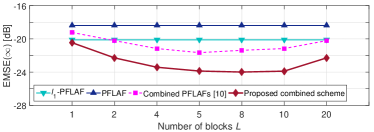
Figure 2: Steady-state EMSE of the proposed method on varying the number of blocks in the combination.

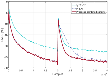
(a)

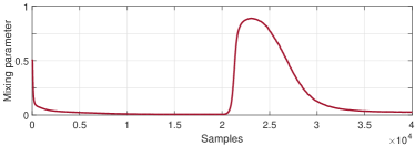
(b)

Figure 3: (a) Convergence behavior in terms of the EMSE of the proposed combined FLAF with $L=8$ and (b) related mixing parameter evolution of the first block.

We evaluate the steady-state performance in the case of strong nonlinearity level ($\zeta=0.03$). Results are depicted in Fig. 2, where the values of the steady-state EMSE are shown on varying the number of blocks from $L=1$, which implies the adaptation of a full block with size $M_{\text{b}}=Q_{\mbox{\tiny${\rm{f}}$}}=40$, to $L=20$, which implies the adaptation of blocks with size $M_{\text{b}}=Q_{\mbox{\tiny${\rm{f}}$}}/L=2$. We compare the performance of the proposed scheme with that of individual sparse FLAFs involving $\ell_{1}$ and proportionate regularization separately, and the performance of the same scheme involving the combination of two PFLAFs (i.e., the algorithm cPSFLAF#1 in [10]). Results show that the use of a blockwise combination (i.e., $L>1$) always produces better results with respect to the full-block combination. The best performance is achieved with $L=8$, which gains about $4$ dB over the same algorithm with $L=1$. Reducing too much the block size leads to a performance decrease, due to gradient noise in the adaptation of the mixing parameters, and also to a computational cost increase.

We also assess the tracking performance by setting two different nonlinearity levels: $\zeta=0.08$ for the first half of the experiment and $\zeta=0.05$ (i.e., stronger nonlinearity) for the second half. Results in Fig. 3LABEL:sub@fig:exp1_emse_behavior, show the improvement of the proposed method (with $L=8$) over the other ones. In particular, it takes advantage of the steady-state performance of the sparse PFLAF, while it exploits the faster convergence rate provided by the $\ell_{1}$-sparse PFLAF when nonlinearity changes. This result is also confirmed by the mixing parameter evolution, depicted in Fig. 3LABEL:sub@fig:exp1_emse_mixpar for the first block.

VI Conclusion

In this paper, a combined sparse regularization scheme for LIP nonlinear filters has been developed based on an $\ell_{1}$-norm proportionate and a classic proportionate sparsity. The proposed method involves a blockwise adaptive combinations of sparse FLAFs having different adaptation rules aiming at improving the overall modeling performance. Experimental results have shown the effectiveness and robustness of our proposal in a time-varying nonlinear system identification problem.

References

- [1] Y. Huang, J. Benesty, and J. Chen, Eds., Acoustic MIMO Signal Processing, ser. Signals and Communication Technology. Berlin, Heildelberg: Springer-Verlag, 2006.
- [2] E. Panayirci, H. Senol, M. Uysal, and H. V. Poor, “Sparse channel estimation and equalization for OFDM-based underwater cooperative systems with amplify-and-forward relaying,” IEEE Trans. Signal Process., vol. 64, no. 1, pp. 214–228, Jan. 2016.
- [3] J. K. Pant and S. Krishnan, “Two-pass p-regularized least-squares algorithm for compressive sensing,” in IEEE Int. Symp. Circuits and Syst. (ISCAS), Baltimore, MD, May 2017, pp. 1–4.
- [4] B. Lei, P. Yang, T. Wang, S. Chen, and D. Ni, “Relational-regularized discriminative sparse learning for Alzheimer’s disease diagnosis,” IEEE Trans. Cybern., vol. 47, no. 4, pp. 1102–1112, Apr. 2017.
- [5] M. Masood, L. H. Afify, and T. Y. Al-Naffouri, “Efficient coordinated recovery of sparse channels in massive MIMO,” IEEE Trans. Signal Processing, vol. 63, no. 1, pp. 104–118, Jan. 2015.
- [6] Y. Shi, J. Zhang, and K. B. Letaief, “Robust group sparse beamforming for multicast green cloud-RAN with imperfect CSI,” IEEE Trans. Signal Process., vol. 63, no. 17, pp. 4647–4659, Sep. 2015.
- [7] J. F. de Andrade, Jr., M. L. R. de Campos, and J. A. Apolinário, Jr., “ -constrained normalized LMS algorithms for adaptive beamforming,” IEEE Trans. Signal Process., vol. 63, no. 24, pp. 6524–6539, Dec. 2015.
- [8] S. Scardapane, D. Comminiello, A. Hussain, and A. Uncini, “Group sparse regularization for deep neural networks,” Neurocomputing, vol. 241, pp. 81–89, Jun. 2017.
- [9] D. Comminiello and J. C. Príncipe, Eds., Adaptive Learning Methods for Nonlinear System Modeling. Elsevier, Jun. 2018, ISBN: 987-0-12-812976-0.
- [10] D. Comminiello, M. Scarpiniti, L. A. Azpicueta-Ruiz, J. Arenas-García, and A. Uncini, “Combined nonlinear filtering architectures involving sparse functional link adaptive filters,” Signal Process., vol. 135, pp. 168–178, Jun. 2017.
- [11] ——, “Nonlinear acoustic echo cancellation based on sparse functional link representations,” IEEE/ACM Trans. Audio, Speech, Language Process., vol. 7, no. 22, pp. 1172–1183, Jul. 2014.
- [12] J. A. Bazerque and G. B. Giannakis, “Nonparametric basis pursuit via sparse kernel-based learning: A unifying view with advances in blind methods,” IEEE Signal Process. Mag., vol. 30, no. 4, pp. 112–125, Jul. 2013.
- [13] W. Liu, I. Park, and J. C. Príncipe, “An information theoretic approach of designing sparse kernel adaptive filters,” IEEE Trans. Neural Netw., vol. 20, no. 12, pp. 1950–1961, Dec. 2009.
- [14] V. Kekatos and G. B. Giannakis, “Sparse Volterra and polynomial regression models: Recoverability and estimation,” IEEE Trans. Signal Process., vol. 59, no. 12, pp. 5907–5920, Dec. 2011.
- [15] D. Comminiello, M. Scarpiniti, L. A. Azpicueta-Ruiz, J. Arenas-García, and A. Uncini, “A block-based combined scheme exploiting sparsity in nonlinear acoustic echo cancellation,” in IEEE Int. Workshop Mach. Learning and Signal Process. (MLSP), Vietri Sul Mare, Italy, 2016, pp. 1–6.
- [16] ——, “Full proportionate functional link adaptive filters for nonlinear acoustic echo cancellation,” in 25th Eur. Signal Process. Conf. (EUSIPCO), Kos Island, Greece, Aug. 2017, pp. 1185–1189.
- [17] G. L. Sicuranza and A. Carini, “A generalized FLANN filter for nonlinear active noise control,” IEEE Trans. Audio, Speech, Language Process., vol. 19, no. 8, pp. 2412–2417, Nov. 2011.
- [18] D. Comminiello, M. Scarpiniti, L. A. Azpicueta-Ruiz, J. Arenas-García, and A. Uncini, “Functional link adaptive filters for nonlinear acoustic echo cancellation,” IEEE Trans. Audio, Speech, Language Process., vol. 21, no. 7, pp. 1502–1512, Jul. 2013.
- [19] V. Patel, V. Gandhi, S. Heda, and N. V. George, “Design of adaptive exponential functional link network-based nonlinear filters,” IEEE Trans. Circuits Syst. I, Reg. Papers, vol. 63, no. 9, pp. 1434–1442, Sep. 2016.
- [20] A. Carini and D. Comminiello, “Introducing complex functional link polynomial filters,” in 42nd IEEE Int. Conf. Acoustics, Speech, Signal Process. (ICASSP), New Orleans, LA, Mar. 5-9 2017, pp. 4656–4660.
- [21] R. Tibshirani, “Regression shrinkage and selection via the lasso,” J. Royal. Statist. Soc. B, vol. 58, no. 1, pp. 267–288, 1996.
- [22] D. Comminiello, M. Scarpiniti, S. Scardapane, and A. Uncini, “Sparse functional link adaptive filter using an -norm regularization,” in IEEE Int. Symp. Circuits and Syst. (ISCAS), Florence, Italy, 2018, pp. 1–4.
- [23] Y. Chen, Y. Gu, and A. O. Hero, “Sparse LMS for system identification,” in IEEE Int. Conf. Acoust., Speech and Signal Process. (ICASSP), Taipei,Taiwan, Apr. 2009, pp. 3125–3128.
- [24] J. Chen, C. Richard, Y. Song, and D. Brie, “Transient performance analysis of zero-attracting LMS,” IEEE Signal Process. Lett., vol. 23, no. 12, pp. 1786–1790, 2016.
- [25] R. L. Das and M. Chakraborty, “Improving the performance of the PNLMS algorithm using norm regularization,” IEEE/ACM Trans. Audio, Speech, Language Process., vol. 24, no. 7, pp. 1280–1290, Jul. 2016.
- [26] J. Arenas-García, L. A. Azpicueta-Ruiz, M. T. M. Silva, V. H. Nascimento, and A. H. Sayed, “Combinations of adaptive filters: Performance and convergence properties,” IEEE Signal Process. Mag., vol. 33, no. 1, pp. 120–140, Jan. 2016.
- [27] D. Comminiello, M. Scarpiniti, R. Parisi, and A. Uncini, “Combined adaptive beamforming schemes for nonstationary interfering noise reduction,” Signal Process., vol. 93, no. 12, pp. 3306–3318, Dec. 2013.
- [28] E. J. Candés, M. Wakin, and S. Boyd, “Enhancing sparsity by reweighted minimization,” J. Fourier Anal. Appl., vol. 14, no. 5-6, pp. 877–905, Dec. 2008.
- [29] C. Paleologu, J. Benesty, and S. Ciochină, “A variable step-size affine projection algorithm dedesign for acoustic echo cancellation,” IEEE Trans. Audio, Speech, Language Process., vol. 16, no. 8, pp. 1466–1478, Nov. 2008.
- [30] J. Benesty and S. L. Gay, “An improved PNLMS algorithm,” in IEEE Int. Conf. Acoust., Speech and Signal Process. (ICASSP), vol. 2, Orlando, FL, May 2002, pp. 1881–1884.