On partial Steiner $(n,r,\ell)$-system process

Abstract

For given integers $r$ and $\ell$ such that $2\leqslant\ell\leqslant r-1$, an $r$-uniform hypergraph $H$ is called a partial Steiner $(n,r,\ell)$-system, if every subset of size $\ell$ lies in at most one edge of $H$. In particular, partial Steiner $(n,r,2)$-systems are also called linear hypergraphs. The partial Steiner $(n,r,\ell)$-system process starts with an empty hypergraph on vertex set $[n]$ at time $0$, the $\binom{n}{r}$ edges arrive one by one according to a uniformly chosen permutation, and each edge is added if and only if it does not overlap any of the previously-added edges in $\ell$ or more vertices. In this paper, we show with high probability, independent of $\ell$, the sharp threshold of connectivity in the algorithm is $\frac{n}{r}\log n$ and the very edge which links the last isolated vertex with another vertex makes the partial Steiner $(n,r,\ell)$-system connected.

Keywords: asymptotic enumeration, graph process, linear hypergraph, connectivity.

hitting time, connectivity.

Mathematics Subject Classifications: 05A16, 05D40

1 Introduction

Hypergraphs, which are also known as set systems and block designs, are fundamental to the study of complex discrete systems. Let $r$ and $\ell$ be given integers such that $2\leqslant\ell\leqslant r-1$. A hypergraph ${H}$ on vertex set $[n]$ is an $r$-uniform hypergraph ($r$-graph for short) if each edge is a set of $r$ vertices. An $r$-graph is called a Steiner $(n,r,\ell)$-system, if every subset of size $\ell$ ($\ell$-set for short) lies in exactly one edge of $H$. Replacing “exactly one edge” by “at most one edge”, we have a partial Steiner $(n,r,\ell)$-system. In particular, partial Steiner $(n,r,2)$-systems are also called linear hypergraphs, and Steiner $(n,3,2)$-systems are called Steiner triple systems. Let $\mathcal{H}_{r}(n,m)$ denote the set of $r$-graphs with $m$ edges, $\mathcal{L}_{r}^{\ell}(n,m)$ denote the set of partial Steiner $(n,r,\ell)$-systems in $\mathcal{H}_{r}(n,m)$, and $\mathcal{L}_{r}^{2}(n,m)$ is specially denoted as $\mathcal{L}_{r}(n,m)$.

The uniform hypergraph process $\mathbb{H}_{r}(n,m)$ is a Markov process with time running through the set $\{0,1,\cdots,\binom{n}{r}\}$. It is the typical random graph process $\mathbb{G}(n,m)$ introduced by Erdős and Rényi when $r=2$ [5]. Similarly, the partial Steiner $(n,r,\ell)$-system process begins with no edges on vertex set $[n]$ at time $0$, all $r$-sets arrive one by one according to a uniformly chosen permutation, and each one is added if and only if it does not overlap any of the previously-added edges in $\ell$ or more vertices. In particular, it is the linear hypergraph process when $\ell=2$. Let $\mathbb{L}_{r}^{\ell}(n,m)$ with $2\leqslant\ell\leqslant r-1$ denote the $m$-th stage of the uniform partial Steiner $(n,r,\ell)$-system process, and $\mathbb{L}_{r}^{2}(n,m)$ is also denoted as $\mathbb{L}_{r}(n,m)$.

The hitting time of connectivity is a classic problem which has been extensively studied in the theory of random graph processes. Bollobás and Thomason [4] proved that, with probability approaching to $1$ when $n\rightarrow\infty$ (w.h.p. for short), $m=\frac{n}{2}\log n$ is a sharp threshold of connectivity for $\mathbb{G}(n,m)$ and the very edge which links the last isolated vertex with another vertex makes the graph connected. Poole [10] proved the analogous result for $\mathbb{H}_{r}(n,m)$ when $r\geqslant 3$ is a fixed integer, which means that $m=\frac{n}{r}\log n$ is the hitting time of connectivity for $\mathbb{H}_{r}(n,m)$. The proofs in [4, 10] are due to the fact that the $m$-th stage $\mathbb{H}_{r}(n,m)$ can be identified with the uniform random hypergraph from $\mathcal{H}_{r}(n,m)$, and behaves in a similar fashion when $m$ equals or is close to the expected number of edges of $\mathbb{H}_{r}(n,p)$, where a random $r$-graph $\mathbb{H}_{r}(n,p)$ is an $r$-graph on the vertex set $[n]$ and each $r$-set is an edge independently with probability $p$.

It might be surmised that the threshold of connectivity for $\mathbb{L}_{r}^{\ell}(n,m)$ is smaller than the one for $\mathbb{H}_{r}(n,m)$ because of its constraint on $r$-graphs. Let $\tau_{c}=\min\{m:\mathbb{L}_{r}^{\ell}(n,m)\ \text{is connected}\}$ and $\tau_{o}=\min\{m:\mathbb{L}_{r}^{\ell}(n,m)\ \text{has no isolated vertices}\}$. These two properties are certainly monotone increasing properties, then $\tau_{c}$ and $\tau_{o}$ are well-defined in $\mathbb{L}_{r}^{\ell}(n,m)$. In this paper, for any fixed integers $r$ and $\ell$ with $2\leqslant\ell\leqslant r-1$, we show that $\mathbb{L}_{r}^{\ell}(n,m)$ has the same threshold function of connectivity with $\mathbb{H}_{r}(n,m)$, and $\mathbb{L}_{r}^{\ell}(n,m)$ also becomes connected exactly at the moment when the last isolated vertex disappears.

Theorem 1.1.

For any fixed integers $r$ and $\ell$ with $2\leqslant\ell\leqslant r-1$, w.h.p., $m=\frac{n}{r}\log n$ is a sharp threshold of connectivity for $\mathbb{L}_{r}^{\ell}(n,m)$ and $\tau_{c}=\tau_{o}$ for $\mathbb{L}_{r}^{\ell}(n,m)$.

From the proof of Theorem 1.1, we also have a corollary about the distribution of the number of isolated vertices in $\mathbb{L}_{r}^{\ell}(n,m)$ when $m=\frac{n}{r}\bigl{(}\log n+c_{n})$ and $c_{n}\rightarrow c\in\mathbb{R}$.

Corollary 1.2.

For any fixed integers $r$ and $\ell$ with $2\leqslant\ell\leqslant r-1$, let $m=\frac{n}{r}\bigl{(}\log n+c_{n})$ with $c_{n}\rightarrow c\in\mathbb{R}$. The number of isolated vertices in $\mathbb{L}_{r}^{\ell}(n,m)$ tends in distribution to the Poisson distribution with mean $\exp[-c]$.

In order to prove Theorem 1.1, unlike the proofs in [4, 10], we cannot work in an analogue of the random hypergraph model $\mathbb{H}_{r}(n,p)$, since randomly-chosen independent edges are very unlikely to generate a linear hypergraph. Instead, we will rely on enumeration results in Theorem 1.3 to Theorem 1.5 below.

Little is known about the enumeration of distinct partial Steiner $(n,r,\ell)$-systems with a given number of edges. Hasheminezhad and McKay [7] obtained the asymptotic number of linear hypergraphs with a given number of edges of each size, assuming a constant bound on the edge size and $o(n^{\frac{4}{3}})$ edges. McKay and Tian [9] obtained the asymptotic enumeration formula for the set of $\mathcal{L}_{r}^{\ell}(n,m)$ as far as $m=o(n^{\frac{3}{2}})$. Tian [11] asymptotically determined the number of linear multipartite hypergraphs when the number of edges is $m=o(n^{\frac{4}{3}})$. In fact, we can apply exactly the same approach to obtain an asymptotic formula for $|\mathcal{L}_{r}^{\ell}(n,m)|$ when $3\leqslant\ell\leqslant r-1$ and $m=o(n^{\frac{\ell+1}{2}})$. It turns out that the proof is a little easier when $\ell\geqslant 3$, as only one type of clusters needs to be considered, compared with four clusters in the case $\ell=2$, see [9]. Hence, the asymptotic expression when $\ell\geqslant 3$ is simpler than the corresponding expression when $\ell=2$, so the statements of Theorem 1.3 and Theorem 1.4 cannot be combined.

Let $N_{i}=\binom{n-i}{r}$ for $0\leqslant i\leqslant n$ and $[x]_{t}=x(x-1)\cdots(x-t+1)$ for some positive integer $t$ be the falling factorial. The standard asymptotic notations $o$ and $O$ refer to $n\rightarrow\infty$. The floor and ceiling signs are omitted whenever they are not crucial.

Theorem 1.3.

([9], Theorem 1.1) For a fixed integer $r\geqslant 3$, let $m=m(n)$ be an integer with $m=o(n^{\frac{3}{2}})$. Then, as $n\rightarrow\infty$,

$$|\mathcal{L}_{r}(n,m)| ={\frac{N_{0}^{m}}{m!}}\exp\biggl{[}-\frac{[r]_{2}^{2}[m]_{2}}{4n^{2}}-\frac{[r]_{2}^{3}(3r^{2}-15r+20)m^{3}}{24n^{4}}+O\Bigl{(}\frac{m^{2}}{n^{3}}\Bigr{)}\biggr{]}.$$

Theorem 1.4.

For fixed integers $r$ and $\ell$ such that $3\leqslant\ell\leqslant r-1$, let $m=m(n)$ be an integer with $m=o(n^{\frac{\ell+1}{2}})$. Then, as $n\rightarrow\infty$,

$$|\mathcal{L}_{r}^{\ell}(n,m)| ={\frac{N_{0}^{m}}{m!}}\exp\biggl{[}-\frac{[r]_{\ell}^{2}[m]_{2}}{2\ell!n^{\ell}}+O\Bigl{(}\frac{m^{2}}{n^{\ell+1}}\Bigr{)}\biggr{]}.$$

As one application of Theorem 1.3 and Theorem 1.4, using the same switching method as Theorem 1.4 in [9] when $\ell=2$, we generalize the probability that $H$ contains a given hypergraph as a subhypergraph when $H\in\mathcal{L}_{r}^{\ell}(n,m)$ for $3\leqslant\ell\leqslant r-1$ chosen uniformly at random. At last, we have

Theorem 1.5.

For fixed integers $r$ and $\ell$ such that $2\leqslant\ell\leqslant r-1$, let $m=m(n)$ and $k=k(n)$ be integers with $m=o(n^{\frac{\ell+1}{2}})$ and $k=o\bigl{(}\frac{n^{\ell+1}}{m^{2}}\bigr{)}$. Let $K=K(n)$ be a given $r$-graph in $\mathcal{L}_{r}^{\ell}(n,k)$ and $H\in\mathcal{L}_{r}^{\ell}(n,m)$ be chosen uniformly at random. Then, as $n\rightarrow\infty$,

$$\mathbb{P}[K\subseteq H]=\frac{[m]_{k}}{N_{0}^{k}}\exp\biggl{[}\frac{[r]_{\ell}^{2}k^{2}}{2\ell!n^{\ell}}+O\Bigl{(}\frac{k}{n^{\ell}}+\frac{m^{2}k}{n^{\ell+1}}\Bigr{)}\biggr{]}.$$

The proof of Theorem 1.5 when $3\leqslant\ell\leqslant r-1$ can be found in the appendix.

The remainder of the paper is structured as follows. Notation and auxiliary results are presented in Section 2. In Section 3, we consider Theorem 1.4, where the way to prove them is a refinement of Theorem 1.1 in [9]. In Section 4, we prove Theorem 1.1. The last section concludes the work. The proof of Theorem 1.5 is in the appendix.

2 Notation and auxiliary results

To state our results precisely, we need some definitions. Let $H$ be an $r$-graph in $\mathcal{H}_{r}(n,m)$. For $U\subseteq[n]$, the codegree of $U$ in $H$, denoted by $\operatorname{codeg}({U})$, is the number of edges of $H$ containing $U$. In particular, $\operatorname{codeg}({U})$ is the degree of $v$ in $H$ if $U=\{v\}$ for $v\in[n]$, denoted by $\deg(v)$. Given an integer $\ell$ with $2\leqslant\ell\leqslant r-1$, any $\ell$-set $\{x_{1},\cdots,x_{\ell}\}\subseteq[n]$ in an edge $e$ of $H$ is called a link of $e$ if $\operatorname{codeg}({x_{1},\cdots,x_{\ell}})\geqslant 2$. Two edges $e_{i}$ and $e_{j}$ in $H$ are called linked edges if $|e_{i}\cap e_{j}|\geqslant\ell$. As defined in [9], let $G_{H}$ be a simple graph whose vertices are the edges of $H$, with two vertices of $G$ adjacent iff the corresponding edges of $H$ are linked. An edge induced subgraph of $H$ corresponding to a non-trivial component of $G_{H}$ is called a cluster of $H$.

Furthermore, for two positive-valued functions $f$, $g$ on the variable $n$, we write $f\ll g$ to denote $\lim_{n\rightarrow\infty}f(n)/g(n)=0$, $f\sim g$ to denote $\lim_{n\rightarrow\infty}f(n)/g(n)=1$ and $f\lesssim g$ if and only if $\lim_{n\rightarrow\infty}\sup f(n)/g(n)\leqslant 1$ . For an event $A$ and a random variable $Z$ in an arbitrary probability space $(\Omega,\mathcal{F},\mathbb{P})$, $\mathbb{P}[A]$ and $\mathbb{E}[Z]$ denote the probability of $A$ and the expectation of $Z$. An event is said to occur with high probability (w.h.p. for short), if the probability that it holds tends to 1 as $n\rightarrow\infty$.

In order to identify several events which have low probabilities in the uniform probability space $\mathcal{H}_{r}(n,m)$ as $m=o(n^{\frac{\ell+1}{2}})$, the following two lemmas will be useful.

Lemma 2.1 ([9], Lemma 2.1).

Let $t=t(n)\geqslant 1$ be an integer and $e_{1},\ldots,e_{t}$ be distinct $r$-sets of $[n]$. For any given integer $r\geqslant 3$, let $H$ be an $r$-graph that is chosen uniformly at random from $\mathcal{H}_{r}(n,m)$. Then the probability that $e_{1},\ldots,e_{t}$ are edges of $H$ is at most $\bigl{(}\frac{m}{N}\bigr{)}^{t}$.

Lemma 2.2 ([9], Lemma 2.2).

Let $r$, $t$ and $\alpha$ be integers such that $r,t,\alpha=O(1)$ and $0\leqslant\alpha\leqslant rt$. If a hypergraph $H$ is chosen uniformly at random from $\mathcal{H}_{r}(n,m)$, then the expected number of sets of $t$ edges of $H$ whose union has $rt-\alpha$ or fewer vertices is $O\bigl{(}m^{t}n^{-\alpha})$.

We will need the following Lemma 2.3 from [6] to find the enumeration formula of $\mathcal{L}_{r}^{\ell}(n,m)$.

Lemma 2.3 ([6], Corollary 4.5).

Let $N\geqslant 2$ be an integer, and for $1\leqslant i\leqslant N$, let real numbers $A(i)$, $B(i)$ be given such that $A(i)\geqslant 0$ and $1-(i-1)B(i)\geqslant 0$. Define $A_{1}=\min_{i=1}^{N}A(i)$, $A_{2}=\max_{i=1}^{N}A(i)$, $C_{1}=\min_{i=1}^{N}A(i)B(i)$ and $C_{2}=\max_{i=1}^{N}A(i)B(i)$. Suppose that there exists a real number $\hat{c}$ with $0<\hat{c}<\frac{1}{3}$ such that $\max\{A/N,|C|\}\leqslant\hat{c}$ for all $A\in[A_{1},A_{2}]$, $C\in[C_{1},C_{2}]$. Define $n_{0}$, $n_{1}$, $\cdots$, $n_{N}$ by $n_{0}=1$ and

$$\frac{n_{i}}{n_{i-1}}=\frac{A(i)}{i}(1-(i-1)B(i))$$

for $1\leqslant i\leqslant N$, with the following interpretation: if $A(i)=0$ or $1-(i-1)B(i)=0$, then $n_{j}=0$ for $i\leqslant j\leqslant N$. Then $\Sigma_{1}\leqslant\sum_{i=0}^{N}n_{i}\leqslant\Sigma_{2}$, where $\Sigma_{1}=\exp[A_{1}-\frac{1}{2}A_{1}C_{2}]-(2e\hat{c})^{N}$ and $\Sigma_{2}=\exp[A_{2}-\frac{1}{2}A_{2}C_{1}+\frac{1}{2}A_{2}C_{1}^{2}]+(2e\hat{c})^{N}$.

3 Enumeration of $\mathcal{L}_{r}^{\ell}(n,m)$

In this section, we first consider the asymptotic enumeration formula for $\mathcal{L}_{r}^{\ell}(n,m)$ as $3\leqslant\ell\leqslant r-1$ and $m=o(n^{\frac{\ell+1}{2}})$ to extend the case of $\ell=2$ and $m=o(n^{\frac{3}{2}})$ in [9]. It turns out that the proof is a little easier when $\ell\geqslant 3$, as only one type of clusters needs to be considered, compared with four clusters in the case $\ell=2$. We remark that the proof follows along the same line of [2, 6, 9, 11] and we are only giving the details here for the sake of self-completeness.

Let $\mathbb{P}(n,r,\ell;m)$ denote the probability that an $r$-graph $H\in\mathcal{H}_{r}(n,m)$ chosen uniformly at random is a partial Steiner $(n,r,\ell)$-system. Then $|\mathcal{L}_{r}^{\ell}(n,m)|={\binom{N}{m}}\mathbb{P}(n,r,\ell;m)$. Our task is reduced to show that $\mathbb{P}(n,r,\ell;m)$ equals the later factor in Theorem 1.4.

Let $\mathcal{L}_{r}^{\ell,+}(n,m)\subset\mathcal{H}_{r}(n,m)$ be the set of $r$-graphs $H$ which satisfy the following properties $\bf(a)$ and $\bf(b)$. We show that the expected number of $r$-graphs in $\mathcal{H}_{r}(n,m)$ not satisfying the properties of $\mathcal{L}_{r}^{\ell,+}(n,m)$ is quite small such that the removal of these $r$-graphs from our main proof will lead to some simplifications.

$\bf(a)$  Every cluster of $H$ consists of two edges overlapping by $\ell$ vertices (Figure 1).

$\bf(b)$  The number of clusters in $H$ is at most $M$, where $M=\bigl{\lceil}\log n+\frac{3^{\ell+2}r^{2\ell}m^{2}}{\ell!n^{\ell}}\bigr{\rceil}$.

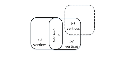
Figure 1: The cluster of $H\in\mathcal{L}_{r}^{\ell,+}(n,m)$.

Lemma 3.1.

For any given integers $r$ and $\ell$ such that $3\leqslant\ell\leqslant r-1$, let $m=m(n)$ be integers with $m=o(n^{\frac{\ell+1}{2}})$. Then, as $n\rightarrow\infty$,

$$\frac{|\mathcal{L}_{r}^{\ell,+}(n,m)|}{|\mathcal{H}_{r}(n,m)|}=1-O\Bigl{(}\frac{m^{2}}{n^{\ell+1}}\Bigr{)}.$$

Proof.

Consider $H\in\mathcal{H}_{r}(n,m)$ chosen uniformly at random. We apply Lemma 2.2 several times to show that $H$ satisfies the properties $\bf(a)$ and $\bf(b)$ with probability $1-O(\frac{m^{2}}{n^{\ell+1}})$.

If two edges overlap by $\ell+1$ or more vertices, then they have at most $2r-\ell-1$ vertices in total, which has probability $O(\frac{m^{2}}{n^{\ell+1}})$ by Lemma 2.2. Similarly if there is a cluster of more than two edges, then three of those edges have at most $3r-2\ell$ vertices in total, which has probability $O(\frac{m^{3}}{n^{2\ell}})=O(\frac{m^{2}}{n^{\ell+1}})$ as $m=o(n^{\frac{\ell+1}{2}})$ and $\ell\geqslant 3$. Therefore, $H$ satisfies the property $\bf(a)$ with probability $1-O(\frac{m^{2}}{n^{\ell+1}})$.

Note that if $\bf(a)$ holds, all clusters have two edges and no two clusters share an edge or a link. Define the event $\mathcal{E}=\{{\rm{There\ are\ at\ least}}\ d\ \text{edge- and }\text{link-disjoint }{\rm{clusters\ in}}\ H\}$, where $d=M+1$. Let $\{x_{1}^{i},\cdots,x_{\ell}^{i}\}\subseteq\binom{[n]}{\ell}$ be a set of links with edges $e_{i}$ and $e_{i}^{\prime}$ for $1\leqslant i\leqslant d$. By Lemma 2.1, we have

$$\mathbb{P}[\mathcal{E}]=O\biggl{(}\binom{n}{r-\ell}^{2d}\binom{\binom{n}{\ell}}{d}\Bigl{(}\frac{m}{N_{0}}\Bigr{)}^{2d}\biggr{)}=O\biggl{(}\biggl{(}\frac{r^{2\ell}em^{2}}{d\ell!n^{\ell}}\biggr{)}^{d}\biggr{)}=O\Bigl{(}\frac{1}{n^{\ell+1}}\Bigr{)},$$

where the last two equalities are true because $d>\frac{3^{\ell+2}r^{2\ell}m^{2}}{\ell!n^{\ell}}$ and $d>\log n$. The proof is complete on noting that the event “$\bf(a)$ and $\bf(b)$” is contained in the union of the event “$\bf(a)$ holds” and “$\mathcal{E}$ doesn’t hold”. ∎

For a nonnegative integer $t$, define $\mathcal{L}_{r}^{\ell,+}(t)$ to be the set of $r$-graphs $H\in\mathcal{S}_{r}^{\ell,+}(n,m)$ with exactly $t$ clusters and we have $|\mathcal{L}_{r}^{\ell,+}(n,m)|=\sum_{t=0}^{M}|\mathcal{L}_{r}^{\ell,+}(t)|$. By Lemma 3.1, we have $|\mathcal{L}_{r}^{\ell,+}(n,m)|\neq 0$ and there exists $t$ such that $|\mathcal{L}_{r}^{\ell,+}(t)|\neq 0$. Note that $\mathcal{L}_{r}^{\ell}(n,m)=\mathcal{L}_{r}^{\ell,+}(0)\neq\emptyset$, then it follows that

$$\frac{1}{\mathbb{P}(n,r,\ell;m)} =\Bigl{(}1-O\Bigl{(}\frac{m^{2}}{n^{\ell+1}}\Bigr{)}\Bigr{)}\sum_{t=0}^{M}\frac{|\mathcal{L}_{r}^{\ell,+}(t)|}{|\mathcal{L}_{r}^{\ell}(n,m)|}=\Bigl{(}1-O\Bigl{(}\frac{m^{2}}{n^{\ell+1}}\Bigr{)}\Bigr{)}\sum_{t=0}^{M}\frac{|\mathcal{L}^{\ell,+}(t)|}{|\mathcal{L}^{\ell,+}(0)|}.$$ (3.1)

In order to calculate the ratio $|\mathcal{L}_{r}^{\ell,+}(t)|/|\mathcal{L}_{r}^{\ell,+}(0)|$ when $1\leqslant t\leqslant M$. We design switchings to find a relationship between the sizes of $\mathcal{L}_{r}^{\ell,+}(t)$ and $\mathcal{L}_{r}^{\ell,+}(t-1)$. Let $H\in\mathcal{L}_{r}^{\ell,+}(t)$. A forward switching from $H$ is used to reduce the number of clusters in $H$. Take any cluster $\{e,f\}$ and remove it from $H$. Define $H_{0}$ with the same vertex set $[n]$ and the edge set $E(H_{0})=E(H)\setminus\{e,f\}$. Take any $r$-set from $[n]$ of which no $\ell$ vertices belong to the same edge of $H_{0}$ and add it as a new edge. The graph is denoted by $H^{\prime}$. Insert another new edge at an $r$-set of $[n]$ again of which no $\ell$ vertices belong to the same edge of $H^{\prime}$. The resulting graph is denoted by $H^{\prime\prime}$. The two new edges in forward switching may have at most $\ell-1$ vertices in common and the operation reduces the number of clusters in $H$ by one. A reverse switching is the reverse of a forward switching. A reverse switching from $H^{\prime\prime}\in\mathcal{L}_{r}^{\ell,+}(t-1)$ is defined by sequentially removing two edges of $H^{\prime\prime}$ not containing a link, then choosing a $(2r-\ell)$-set $T$ from $[n]$ such that no $\ell$ vertices belong to any remaining edge of $H^{\prime\prime}$, then inserting two edges into $T$ such that they create a cluster.

Lemma 3.2.

For any given integers $r$ and $\ell$ such that $3\leqslant\ell\leqslant r-1$, let $m=m(n)$ be an integer with $m=o(n^{\frac{\ell+1}{2}})$. Let $t$ be a positive integer with $1\leqslant t\leqslant M$.
$(a)$ Let $H\in\mathcal{L}_{r}^{\ell,+}(t)$. The number of forward switchings for $H$ is $tN_{0}^{2}(1+O(\frac{m}{n^{\ell}}))$.

$(b)$ Let $H^{\prime\prime}\in\mathcal{L}_{r}^{\ell,+}(t-1)$. The number of reverse switchings for $H^{\prime\prime}$ is $\frac{(2r-\ell)!}{\ell!(r-\ell)!^{2}}\binom{m-2(t-1)}{2}\binom{n}{2r-\ell}(1+O(\frac{m}{n^{\ell}}))$.

Proof.

$(a)$ Let $H\in\mathcal{L}_{r}^{\ell,+}(t)$. Let $\mathcal{R}(H)$ be the set of all forward switchings which can be applied to $H$. There are exactly $t$ ways to choose a cluster. The number of $r$-sets to insert the new edge is at most $N_{0}$. From this we subtract the $r$-sets that have $\ell$ vertices belong to some other edge of $H$, which is at most $\binom{r}{\ell}m\binom{n-\ell}{r-\ell}=O(\frac{m}{n^{\ell}})N_{0}$. Thus, in each step of the forward switching, there are $N_{0}(1+O(\frac{m}{n^{\ell}}))$ ways to choose the new edge and we have $|\mathcal{R}(H)|=tN_{0}^{2}(1+O(\frac{m}{n^{\ell}}))$.

$(b)$ Conversely, suppose that $H^{\prime\prime}\in\mathcal{L}_{r}^{\ell,+}(t-1)$. Similarly, let $\mathcal{R}^{\prime}(H^{\prime\prime})$ be the set of all reverse switchings for $H^{\prime\prime}$. There are exactly $2\binom{m-2(t-1)}{2}$ ways to delete two edges in sequence such that neither of them contain a link. There are at most $\binom{n}{2r-\ell}$ ways to choose a $(2r-\ell)$-set $T$ from $[n]$. From this, we subtract the $(2r-\ell)$-sets that have $\ell$ vertices belong to some other edge of $H^{\prime\prime}$, which is at most $\binom{r}{\ell}m\binom{n-\ell}{2r-2\ell}=O(\frac{m}{n^{\ell}})\binom{n}{2r-\ell}$. For every $T$, there are $\frac{1}{2}\binom{2r-\ell}{\ell}\binom{2r-2\ell}{r-\ell}$ ways to create a cluster in $T$. Thus, we have $|\mathcal{R}^{\prime}(H^{\prime\prime})|=\binom{2r-\ell}{\ell}\binom{2r-2\ell}{r-\ell}\binom{m-2(t-1)}{2}\binom{n}{2r-\ell}(1+O(\frac{m}{n^{\ell}}))$. ∎

Corollary 3.3.

With notation as above, for some $1\leqslant t\leqslant M$, the following hold:
$(a)$ $|\mathcal{L}_{r}^{\ell,+}(t)|>0$ if and only if $m\geqslant 2t$.
$(b)$ Let $t^{\prime}$ be the first value of $t\leqslant M$ such that $\mathcal{L}_{r}^{\ell,+}(t)=\emptyset$, or $t^{\prime}=M+1$ if no such value exists. Then, as $n\rightarrow\infty$, uniformly for $1\leqslant t<t^{\prime}$,

$$\frac{|\mathcal{L}_{r}^{\ell,+}(t)|}{|\mathcal{L}_{r}^{\ell,+}(t-1)|}=\binom{m-2(t-1)}{2}\frac{[r]_{\ell}^{2}}{\ell!tn^{\ell}}\Bigl{(}1+O\Bigl{(}\frac{1}{n}\Bigr{)}\Bigr{)}.$$

Proof.

$(a)$ Firstly, $m\geqslant 2t$ is a necessary condition for $|\mathcal{L}_{r}^{\ell,+}(t)|>0$. By Lemma 3.1, there is some $0\leqslant\hat{t}\leqslant M$ such that $\mathcal{L}_{r}^{\ell,+}(\hat{t})\neq\emptyset$. We can move $\hat{t}$ to $t$ by a sequence of forward and reverse switchings while no greater than $M$. Note that the values given in Lemma 3.2 at each step of this path are positive, we have $|\mathcal{L}_{r}^{\ell,+}(t)|>0$.

$(b)$ By $(a)$, if $\mathcal{L}_{r}^{\ell,+}(t)=\emptyset$, then $\mathcal{L}_{r}^{\ell,+}(t+1),\cdots,\mathcal{L}_{r}^{\ell,+}(M)=\emptyset$. By the definition of $t^{\prime}$, the left hand ratio is well defined. By Lemma 3.2, we complete the proof of $(b)$, where $O(\frac{m}{n^{\ell}})$ is absorbed into $O(\frac{1}{n})$ as $m=o(n^{\frac{\ell+1}{2}})$ and $\ell\geqslant 3$. ∎

At last, by Lemma 2.3, we estimate $\sum_{t=0}^{M}\frac{|\mathcal{L}_{r}^{\ell,+}(t)|}{|\mathcal{L}_{r}^{\ell,+}(0)|}$ in (3.1) to finish the proof of Theorem 1.4.

Lemma 3.4.

For any given integers $r$ and $\ell$ such that $3\leqslant\ell\leqslant r-1$, let $m=m(n)$ be an integer with $m=o(n^{\frac{\ell+1}{2}})$. With notation as above, as $n\rightarrow\infty$,

$$\sum_{t=0}^{M}\frac{|\mathcal{L}_{r}^{\ell,+}(t)|}{|\mathcal{L}_{r}^{\ell,+}(0)|}= \exp\biggl{[}\frac{[r]_{\ell}^{2}[m]_{2}}{2\ell!n^{\ell}}+O\Bigl{(}\frac{m^{2}}{n^{\ell+1}}\Bigr{)}\biggr{]}.$$

Proof.

Let $t^{\prime}$ be as defined in Lemma 3.3(b) and we have shown $|\mathcal{L}_{r}^{\ell,+}(0)|=|\mathcal{L}_{r}^{\ell}(n,m)|\neq 0$, then $t^{\prime}\geqslant 1$. But if $t^{\prime}=1$, by Lemma 3.3(a), we have $m<2$ and the conclusion is obviously true. In the following, suppose $t^{\prime}\geqslant 2$. Define $n_{0},\cdots,n_{M}$ by $n_{0}=1$, $n_{t}=|\mathcal{L}_{r}^{\ell,+}(t)|/|\mathcal{L}_{r}^{\ell,+}(0)|$ for $1\leqslant t<t^{\prime}$ and $n_{t}=0$ for $t^{\prime}\leqslant t\leqslant M$. By Lemma 3.3(b), for $1\leqslant t<t^{\prime}$, we have

$$\frac{n_{t}}{n_{t-1}} =\frac{1}{t}\binom{m-2(t-1)}{2}\frac{[r]_{\ell}^{2}}{\ell!n^{\ell}}\Bigl{(}1+O\Bigl{(}\frac{1}{n}\Bigr{)}\Bigr{)}.$$ (3.2)

For $1\leqslant t\leqslant M$, define

$$A(t) =\frac{[r]_{\ell}^{2}[m]_{2}}{2\ell!n^{\ell}}\Bigl{(}1+O\Bigl{(}\frac{1}{n}\Bigr{)}\Bigr{)},$$ (3.3)

$$B(t) =\begin{cases}\frac{2(2m-2t+1)}{m(m-1)},\text{for}\ 1\leqslant t<t^{\prime};\\ (t-1)^{-1},\text{otherwise}.\end{cases}$$

As the equations shown in (3.2) and (3.3), we further have $\frac{n_{{t}}}{n_{t-1}}=\frac{A(t)}{t}(1-(t-1)B(t))$.

Following the notation of Lemma 2.3, we have $A_{1},A_{2}=\frac{[r]_{\ell}^{2}[m]_{2}}{2\ell!n^{\ell}}(1+O(\frac{1}{n}))$. For $1\leqslant t<t^{\prime}$, we have $A(t)B(t)=\frac{[r]_{\ell}^{2}(2m-2t+1)}{\ell!n^{\ell}}(1+O(\frac{1}{n}))$. Thus, we have $A(t)B(t)=O(\frac{m}{n^{\ell}})$ for $1\leqslant t<t^{\prime}$. For the case $t^{\prime}\leqslant t\leqslant M$ and $t^{\prime}\geqslant 2$, by Lemma 3.3(a), we have $2\leqslant m<2t$. As the equation shown in (3.3), we also have $A(t)B(t)=O(\frac{m}{n^{\ell}})$ for $t^{\prime}\leqslant t\leqslant M$. In both cases, we have $C_{1},C_{2}=O(\frac{m}{n^{\ell}})$. Note that $|C|=o(1)$ for all $C\in[C_{1},C_{2}]$ as $m=o(n^{\frac{\ell+1}{2}})$.

Let $\hat{c}=\frac{1}{2(3^{\ell+2})}$, then $\max\{A/M,|C|\}\leqslant\hat{c}<\frac{1}{3}$ and $(2e\hat{c})^{M}=O(\frac{1}{n^{\ell+1}})$ as $n\rightarrow\infty$. Lemma 2.3 applies to obtain $\sum_{t=0}^{M}\frac{|\mathcal{L}_{r}^{\ell,+}(t)|}{|\mathcal{L}_{r}^{\ell,+}(0)|}=\exp\bigl{[}\frac{[r]_{\ell}^{2}[m]_{2}}{2\ell!n^{\ell}}+O\bigl{(}\frac{m^{2}}{n^{\ell+1}}\bigr{)}\bigr{]}$, where $O(\frac{m^{3}}{n^{2\ell}})=O(\frac{m^{2}}{n^{\ell+1}})$ as $m=o(n^{\frac{\ell+1}{2}})$. ∎

Proof of Theorem 1.4.

By Lemma 3.4, as the equation shown in (3.1),

$$|\mathcal{L}_{r}^{\ell}(n,m)| =\binom{N_{0}}{m}\exp\Bigl{[}-\frac{[r]_{\ell}^{2}[m]_{2}}{2\ell!n^{\ell}}+O\Bigl{(}\frac{m^{2}}{n^{\ell+1}}\Bigr{)}\Bigr{]}$$

$$=\frac{N_{0}^{m}}{m!}\exp\Bigl{[}-\frac{[r]_{\ell}^{2}[m]_{2}}{2\ell!n^{\ell}}+O\Bigl{(}\frac{m^{2}}{n^{\ell+1}}\Bigr{)}\Bigr{]},$$

where $\binom{N_{0}}{m}=\frac{N_{0}^{m}}{m!}\exp\bigl{[}O\bigl{(}\frac{m^{2}}{N_{0}}\bigr{)}\bigr{]}=\frac{N_{0}^{m}}{m!}\exp\bigl{[}O\bigl{(}\frac{m^{2}}{n^{\ell+1}}\bigr{)}\bigr{]}$. We complete the proof of Theorem 1.4. ∎

Remark 3.5.

We also extend the probability that a random linear $r$-graph with $m=o(n^{\frac{3}{2}})$ edges contains a given subhypergraph (Theorem 1.4 in [9]), by similar discussions with appropriate modifications, to the case $3\leqslant\ell\leqslant r-1$ and $m=o(n^{\frac{\ell+1}{2}})$. We show it in the Appendix for reference.

4 Connectivity for $\mathbb{L}_{r}^{\ell}(n,m)$

As one application of Theorem 1.3 to Theorem 1.5, we consider the hitting time of connectivity for partial Steiner $(n,r,\ell)$-system process $\mathbb{L}_{r}^{\ell}(n,m)$ for any given integers $r$ and $\ell$ with $2\leqslant\ell\leqslant r-1$. It is clear that $\tau_{o}\leqslant\tau_{c}$. Let

$$m_{L}=\frac{n}{r}(\log n-\omega(n))\quad\text{and}\quad m_{R}=\frac{n}{r}(\log n+\omega(n)),$$ (4.1)

where $\omega(n)\rightarrow\infty$ sufficiently slowly when $n\rightarrow\infty$ and taking $\omega(n)=\log\log n$ for convenience.

We prove our main result Theorem 1.1 from a sequence of lemmas which we show next.

Lemma 4.1.

Let $H$ be chosen from $\mathcal{L}_{r}^{\ell}(n,m)$ uniformly at random when $m=o(n^{\frac{\ell+1}{2}})$, and $v_{1},\cdots,v_{t}\in[n]$ be $t$ distinct vertices for some fixed integer $t\geqslant 1$. Then, as $n\rightarrow\infty$,

$$\mathbb{P}\bigl{[}\deg(v_{1})=\cdots=\deg(v_{t})=0\bigr{]}=\exp\Bigl{[}-\frac{trm}{n}+O\Bigl{(}\frac{m}{n^{2}}+\frac{m^{2}}{n^{\ell+1}}\Bigr{)}\Bigr{]}.$$

Proof.

By Theorem 1.3 and Theorem 1.4, for one vertex $v\in[n]$, we have

$$\mathbb{P}\bigl{[}\deg(v)=0\bigr{]} =\frac{|\mathcal{L}_{r}^{\ell}(n-1,m)|}{|\mathcal{L}_{r}^{\ell}(n,m)|}=\frac{N_{1}^{m}}{N_{0}^{m}}\exp\biggl{[}O\Bigl{(}\frac{m^{2}}{n^{\ell+1}}\Bigr{)}\biggr{]}$$

$$=\exp\biggl{[}-\frac{rm}{n}+O\Bigl{(}\frac{m}{n^{2}}+\frac{m^{2}}{n^{\ell+1}}\Bigr{)}\biggr{]},$$

where the last equality is true because $\frac{N_{1}}{N_{0}}=\exp[-\frac{r}{n}+O(\frac{1}{n^{2}})]$. Thus, for a fixed integer $t\geqslant 1$,

$$\mathbb{P}\bigl{[}\deg(v_{1})=\cdots=\deg(v_{t})=0\bigr{]}=\frac{|\mathcal{L}_{r}^{\ell}(n-t,m)|}{|\mathcal{L}_{r}^{\ell}(n,m)|}=\exp\biggl{[}-\frac{trm}{n}+O\Bigl{(}\frac{m}{n^{2}}+\frac{m^{2}}{n^{\ell+1}}\Bigr{)}\biggr{]}$$

to complete the proof of Lemma 4.1. ∎

Lemma 4.2.

Let $H$ be chosen from $\mathcal{L}_{r}^{\ell}(n,m)$ uniformly at random. W.h.p. there are at most $2\log n$ isolated vertices in $H$ when $m=m_{L}$, while w.h.p. there are no isolated vertices in $H$ when $m=m_{R}$. Thus, $\tau_{o}\in[m_{L},m_{R}]$.

Proof.

Let $X_{m}$ be the number of isolated vertices in $H$, where $m\in[m_{L},m_{R}]$. By Lemma 4.1, for any fixed integer $t\geqslant 1$, we have the $t$-th factorial moment of $X_{m}$ is

$$\mathbb{E}[X_{m}]_{t} =[n]_{t}\mathbb{P}\bigl{[}\deg(v_{1})=\cdots=\deg(v_{t})=0\bigr{]}$$

$$=[n]_{t}\exp\biggl{[}-\frac{trm}{n}+O\Bigl{(}\frac{m}{n^{2}}+\frac{m^{2}}{n^{\ell+1}}\Bigr{)}\biggr{]}.$$ (4.2)

For $m=m_{R}$ and $t=1$, we have

$$\mathbb{E}[X_{m_{R}}] =n\exp\biggl{[}-\frac{rm_{R}}{n}+O\Bigl{(}\frac{m_{R}}{n^{2}}+\frac{m_{R}^{2}}{n^{\ell+1}}\Bigr{)}\biggr{]}$$

$$=\exp\Bigl{[}-\omega(n)+O\Bigl{(}\frac{\log n}{n}+\frac{\log^{2}n}{n^{\ell-1}}\Bigr{)}\Bigr{]}$$

$$\rightarrow 0$$

when $n\rightarrow\infty$. Thus, w.h.p., there are no isolated vertices in $H$ when $m=m_{R}$.

For $m=m_{L}$ and $t=1$, we have

$$\mathbb{E}[X_{m_{L}}]=\exp\Bigl{[}\omega(n)+O\Bigl{(}\frac{\log n}{n}+\frac{\log^{2}n}{n^{\ell-1}}\Bigr{)}\Bigr{]}\rightarrow\infty$$ (4.3)

when $n\rightarrow\infty$. For $m=m_{L}$ and $t=2$, using the equations in (4) and (4.3),

$$\mathbb{E}[X_{m_{L}}]_{2} =[n]_{2}\exp\biggl{[}-\frac{2rm_{L}}{n}+O\Bigl{(}\frac{m_{L}}{n^{2}}+\frac{m_{L}^{2}}{n^{\ell+1}}\Bigr{)}\biggr{]}$$

$$=\frac{[n]_{2}}{n^{2}}\exp\biggl{[}2\omega(n)+O\Bigl{(}\frac{m_{L}}{n^{2}}+\frac{m_{L}^{2}}{n^{\ell+1}}\Bigr{)}\biggr{]}$$

$$\sim\mathbb{E}^{2}[X_{m_{L}}].$$

Then, $\mathbb{V}[X_{m_{L}}]\sim\mathbb{E}[X_{m_{L}}]$. By Chebyshev’s inequality and $\mathbb{E}[X_{m_{L}}]\rightarrow\infty$ shown in (4.3), $\mathbb{P}[|X_{m_{L}}-\mathbb{E}[X_{m_{L}}]|\geqslant\mathbb{E}[X_{m_{L}}]]\leqslant\mathbb{V}[X_{m_{L}}]/\mathbb{E}^{2}[X_{m_{L}}]\sim 1/\mathbb{E}[X_{m_{L}}]\rightarrow 0$. Thus, w.h.p., we have at most $2\log n$ isolated vertices in $H$ when $m=m_{L}$ because $X_{m_{L}}$ is concentrated around $\exp[\omega(n)]=\log n$ when $\omega(n)=\log\log n$. ∎

Lemma 4.3.

If $H$ is chosen uniformly at random from $\mathcal{S}(n,r,\ell;m_{L})$, then w.h.p. $H$ has at most $2\log n$ isolated vertices and all remaining vertices are in a giant component.

Proof.

Suppose that $H$ is chosen from $\mathcal{L}_{r}^{\ell}(n,m_{L})$ uniformly at random. By Lemma 4.2, we only prove that w.h.p. all non-isolated vertices in $H$ belong to a giant component.

For any nonnegative integers $k$ and $h$, let $Y_{k,h}$ be the number of components on $k$ vertices with exactly $h$ edges in $H$. By symmetry, we can assume $k\in[r,\frac{n}{2}]$. On one hand, we have $h=h(k)\geqslant\frac{k-1}{r-1}$ because every component is connected and $\frac{k-1}{r-1}$ is the number of edges in a hypertree; on the other hand, $h=h(k)\leqslant\min\bigl{\{}m_{L},\binom{k}{\ell}/\binom{r}{\ell}\bigr{\}}$ because it is also a partial Steiner $(n,r,\ell)$-system. Let

$$h_{\rm{min}}=\frac{k-1}{r-1}\quad{\text{and}}\quad h_{\rm{max}}=\min\Bigl{\{}m_{L},\binom{k}{\ell}/\binom{r}{\ell}\Bigr{\}}.$$ (4.4)

Fix $k\in[r,\frac{n}{2}]$ and choose some $k$-set on $[n]$, then the probability that the $k$-set contains exactly $h$ edges is at most $|\mathcal{L}_{r}^{\ell}(k,h)|\cdot|\mathcal{L}_{r}^{\ell}(n-k,m_{L}-h)|/|\mathcal{L}_{r}^{\ell}(n,m_{L})|$. It is clear that

$$\mathbb{E}[Y_{k,h}] \leqslant\frac{\binom{n}{k}|\mathcal{L}_{r}^{\ell}(k,h)|\cdot|\mathcal{L}_{r}^{\ell}(n-k,m_{L}-h)|}{|\mathcal{L}_{r}^{\ell}(n,m_{L})|}.$$ (4.5)

Let $Y_{k}=\sum_{h_{\rm{min}}\leqslant h\leqslant h_{\rm{max}}}Y_{k,h}$. We will prove

$$\sum_{r\leqslant k\leqslant\frac{n}{2}}\mathbb{E}[Y_{k}]=\sum_{r\leqslant k\leqslant\frac{n}{2}}\sum_{h_{\rm{min}}\leqslant h\leqslant h_{\rm{max}}}\mathbb{E}[Y_{k,h}]\rightarrow 0$$ (4.6)

to show that the remaining vertices in $H$ w.h.p. are all in a giant component.

Define

$$I_{1}=\Bigl{[}r,\frac{n}{\log n}\Bigr{]}\ \text{and}\ I_{2}=\Bigl{[}\frac{n}{\log n},\frac{n}{2}\Bigr{]}.$$ (4.7)

We firstly show $\sum_{k\in I_{1}}\mathbb{E}[Y_{k}]\rightarrow 0$ from Claim 1 to Claim 4, then $\sum_{k\in I_{2}}\mathbb{E}[Y_{k}]\rightarrow 0$ from Claim 5 to Claim 8.

Claim 1.  For any $k\in I_{1}$ and $h_{\rm{min}}\leqslant h\leqslant h_{\rm{max}}$,

$$\bigl{|}\mathcal{L}_{r}^{\ell}(n-k,m_{L}-h)\bigr{|}\sim\frac{N_{k}^{m_{L}-h}}{(m_{L}-h)!}\exp\biggl{[}-\frac{[r]_{\ell}^{2}[m_{L}-h]_{2}}{2\ell!(n-k)^{\ell}}\biggr{]}.$$

Proof of Claim 1.

Note that $n-k\rightarrow\infty$ when $k\in I_{1}$. If $\ell=2$, by Theorem 1.3, we have

$$\bigl{|}\mathcal{L}_{r}^{\ell}(n-k,m_{L}-h)\bigr{|} =\frac{N_{k}^{m_{L}-h}}{(m_{L}-h)!}\exp\biggl{[}-\frac{[r]_{2}^{2}[m_{L}-h]_{2}}{4(n-k)^{2}}+O\biggl{(}\frac{(m_{L}-h)^{3}}{(n-k)^{4}}+\frac{(m_{L}-h)^{2}}{(n-k)^{3}}\biggr{)}\biggr{]}$$

$$\sim\frac{N_{k}^{m_{L}-h}}{(m_{L}-h)!}\exp\biggl{[}-\frac{[r]_{2}^{2}[m_{L}-h]_{2}}{4(n-k)^{2}}\biggr{]},$$

where the last approximate equality is true because $m_{L}=\frac{n}{r}(\log n-\omega(n))$ and $k\in I_{1}$.

If $3\leqslant\ell\leqslant r-1$, by Theorem 1.4, we similarly also have

$$\bigl{|}\mathcal{L}_{r}^{\ell}(n-k,m_{L}-h)\bigr{|} =\frac{N_{k}^{m_{L}-h}}{(m_{L}-h)!}\exp\biggl{[}-\frac{[r]_{\ell}^{2}[m_{L}-h]_{2}}{2\ell!(n-k)^{\ell}}+O\Bigl{(}\frac{(m_{L}-h)^{2}}{(n-k)^{\ell+1}}\Bigr{)}\biggr{]}$$

$$\sim\frac{N_{k}^{m_{L}-h}}{(m_{L}-h)!}\exp\biggl{[}-\frac{[r]_{\ell}^{2}[m_{L}-h]_{2}}{2\ell!(n-k)^{\ell}}\biggr{]}.$$

∎

Claim 2.  For any $k\in I_{1}$ and $h_{\rm{min}}\leqslant h\leqslant h_{\rm{max}}$,

$$\bigl{|}\mathcal{L}_{r}^{\ell}(k,h)\bigr{|}\cdot\bigl{|}\mathcal{L}_{r}^{\ell}(n-k,m_{L}-h)\bigr{|} <\frac{\binom{k}{r}^{h_{{\rm min}}}}{h_{{\rm min}}!}\frac{N_{k}^{m_{L}-h_{{\rm min}}}}{(m_{L}-h_{{\rm min}})!}\exp\biggl{[}-\frac{[r]_{\ell}^{2}[m_{L}-h_{{\rm min}}]_{2}}{2\ell!(n-k)^{\ell}}\biggr{]}.$$

Proof of Claim 2.

Firstly, it is clear that $|\mathcal{L}_{r}^{\ell}(k,h)|\leqslant\binom{\binom{k}{r}}{h}$. By Claim 1, we have

$$\bigl{|}\mathcal{L}_{r}^{\ell}(k,h)\bigr{|}\cdot\bigl{|}\mathcal{L}_{r}^{\ell}(n-k,m_{L}-h)\bigr{|} <\frac{\binom{k}{r}^{h}}{h!}\frac{N_{k}^{m_{L}-h}}{(m_{L}-h)!}\exp\biggl{[}-\frac{[r]_{\ell}^{2}[m_{L}-h]_{2}}{2\ell!(n-k)^{\ell}}\biggr{]}.$$ (4.8)

Let

$$g_{1}(h)=\frac{\binom{k}{r}^{h}}{h!}\frac{N_{k}^{m_{L}-h}}{(m_{L}-h)!}\exp\biggl{[}-\frac{[r]_{\ell}^{2}[m_{L}-h]_{2}}{2\ell!(n-k)^{\ell}}\biggr{]}.$$

Note that

$$\frac{g_{1}(h+1)}{g_{1}(h)} =\frac{\binom{k}{r}}{h+1}\frac{m_{L}-h}{N_{k}}\exp\biggl{[}\frac{[r]_{\ell}^{2}[m_{L}-h]_{2}}{2\ell!(n-k)^{\ell}}-\frac{[r]_{\ell}^{2}[m_{L}-h-1]_{2}}{2\ell!(n-k)^{\ell}}\biggr{]}$$

$$=\frac{\binom{k}{r}}{h+1}\frac{m_{L}-h}{N_{k}}\exp\Bigl{[}O\Bigl{(}\frac{m_{L}}{(n-k)^{\ell}}\Bigr{)}\Bigr{]}.$$

By $h\geqslant h_{{\rm min}}\geqslant\frac{k}{r}$, $m_{L}=\frac{n}{r}(\log n-\omega(n))$ and $\ell\geqslant 2$, we further have

$$\frac{g_{1}(h+1)}{g_{1}(h)} <\frac{\binom{k}{r}}{k}\frac{n\log n}{N_{k}}\exp\Bigl{[}O\Bigl{(}\frac{m_{L}}{(n-k)^{\ell}}\Bigr{)}\Bigr{]}=O\Bigl{(}\frac{k^{r-1}\log n}{n^{r-1}}\Bigr{)},$$

which implies that $\frac{g_{1}(h+1)}{g_{1}(h)}\rightarrow 0$ when $k\in I_{1}$ in (4.7) and $r\geqslant 3$. Thus, $g_{1}(h)$ is decreasing in $h$. Using the equation (4.8) with $h=h_{\rm{min}}$, we complete the proof of Claim 2. ∎

Claim 3.   For any $k\in I_{1}$ and $h_{{\rm min}}\leqslant h\leqslant h_{{\rm max}}$,

$$\mathbb{E}[Y_{k,h}]<\frac{k^{rh_{{\rm min}}}(\log n)^{k+h_{{\rm min}}}}{r^{h_{{\rm min}}}k!h_{{\rm min}}!n^{k-1}}\exp\Bigl{[}\frac{krh_{{\rm min}}}{n}\Bigr{]}.$$

Proof of Claim 3.

By Theorem 1.3 and Theorem 1.4, for $2\leqslant\ell\leqslant r-1$ and $m_{L}=\frac{n}{r}(\log n-\omega(n))$, we also have

$$\bigl{|}\mathcal{L}_{r}^{\ell}(n,m_{L})\bigr{|}\sim\frac{N_{0}^{m_{L}}}{m_{L}!}\exp\biggl{[}-\frac{[r]_{\ell}^{2}[m_{L}]_{2}}{2\ell!n^{\ell}}\biggr{]}.$$

Using the equations shown in (4.5) and Claim 2, it follows that

$$\mathbb{E}[Y_{k,h}] <\frac{\binom{n}{k}\frac{\binom{k}{r}^{h_{{\rm min}}}}{h_{{\rm min}}!}\frac{N_{k}^{m_{L}-h_{{\rm min}}}}{(m_{L}-h_{{\rm min}})!}\exp\Bigl{[}-\frac{[r]_{\ell}^{2}[m_{L}-h_{{\rm min}}]_{2}}{2\ell!(n-k)^{\ell}}\Bigr{]}}{\frac{N_{0}^{m_{L}}}{m_{L}!}\exp\Bigl{[}-\frac{[r]_{\ell}^{2}[m_{L}]_{2}}{2\ell!n^{\ell}}\Bigr{]}}$$

$$<\frac{m_{L}^{h_{{\rm min}}}\binom{n}{k}\binom{k}{r}^{h_{{\rm min}}}N_{k}^{m_{L}-h_{{\rm min}}}}{h_{{\rm min}}!N_{0}^{m_{L}}}\exp\biggl{[}-\frac{[r]_{\ell}^{2}[m_{L}-h_{{\rm min}}]_{2}}{2\ell!(n-k)^{\ell}}+\frac{[r]_{\ell}^{2}[m_{L}]_{2}}{2\ell!n^{\ell}}\biggr{]}$$

$$<\frac{m_{L}^{h_{{\rm min}}}\binom{n}{k}\binom{k}{r}^{h_{{\rm min}}}N_{k}^{m_{L}-h_{{\rm min}}}}{h_{{\rm min}}!N_{0}^{m_{L}}},$$

where the last inequality is true because $\frac{k\ell}{n}-\frac{2h_{{\rm min}}}{m_{L}}>0$ when $k\in I_{1}$ and $m_{L}=\frac{n}{r}(\log n-\omega(n))$, and hence

$$\exp\biggl{[}-\frac{[r]_{\ell}^{2}[m_{L}-h_{{\rm min}}]_{2}}{2\ell!(n-k)^{\ell}}+\frac{[r]_{\ell}^{2}[m_{L}]_{2}}{2\ell!n^{\ell}}\biggr{]}\sim\exp\biggl{[}-\frac{[r]_{\ell}^{2}[m_{L}]_{2}}{2\ell!n^{\ell}}\biggl{(}\frac{k\ell}{n}-\frac{2h_{{\rm min}}}{m_{L}}\biggr{)}\biggr{]}<1.$$

Note that $N_{0}\sim\frac{n^{r}}{r!}$, $N_{k}\sim\frac{(n-k)^{r}}{r!}$, $\binom{n}{k}\sim\frac{n^{k}}{k!}$ and $\binom{k}{r}\leqslant\frac{k^{r}}{r!}$ when $k\in I_{1}$ and $n\rightarrow\infty$, we further have

$$\mathbb{E}[Y_{k,h}] <\frac{m_{L}^{h_{{\rm min}}}k^{rh_{{\rm min}}}(n-k)^{r(m_{L}-h_{{\rm min}})}}{k!h_{{\rm min}}!n^{rm_{L}-k}}.$$ (4.9)

Substituting $m_{L}=\frac{n}{r}(\log n-\log\log n)$ into the above equation, we have $m_{L}^{h_{{\rm min}}}<\frac{n^{h_{{\rm min}}}}{r^{h_{{\rm min}}}}(\log n)^{h_{{\rm min}}}$ and

$$(n-k)^{r(m_{L}-h_{{\rm min}})} \leqslant n^{r(m_{L}-h_{{\rm min}})}\exp\biggl{[}-\frac{kr(m_{L}-h_{{\rm min}})}{n}\biggr{]}$$

$$=\frac{n^{r(m_{L}-h_{{\rm min}})}\log^{k}n}{n^{k}}\exp\biggl{[}\frac{krh_{{\rm min}}}{n}\biggr{]}.$$

Thus, by $(r-1)h_{\rm{min}}=k-1$, the equation in (4.9) is reduced to

$$\mathbb{E}[Y_{k,h}] <\frac{k^{rh_{{\rm min}}}(\log n)^{k+h_{{\rm min}}}}{r^{h_{{\rm min}}}k!h_{{\rm min}}!n^{k-1}}\exp\biggl{[}\frac{krh_{{\rm min}}}{n}\biggr{]}.$$

∎

Claim 4.  $\sum_{k\in I_{1}}\mathbb{E}[Y_{k}]\rightarrow 0$.

Proof of Claim 4.

By the equations in (4.4), Claim 3 and $m_{L}<\frac{n}{r}\log n$, it follows that

$$\mathbb{E}[Y_{k}] =\sum_{h_{{\rm min}}\leqslant h\leqslant h_{{\rm max}}}\mathbb{E}[Y_{k,h}]<\frac{k^{rh_{{\rm min}}}(\log n)^{k+h_{{\rm min}}+1}}{r^{h_{{\rm min}}+1}k!h_{{\rm min}}!n^{k-2}}\exp\biggl{[}\frac{krh_{{\rm min}}}{n}\biggr{]}.$$

Since $h_{\rm{min}}=\frac{k-1}{r-1}\geqslant\frac{k}{r}$ when $k\in I_{1}$, we have $h_{{\rm min}}!\geqslant(\frac{h_{{\rm min}}}{e})^{h_{{\rm min}}}\geqslant(\frac{k}{re})^{h_{{\rm min}}}$. By $k!\geqslant(\frac{k}{e})^{k}$ and $(r-1)h_{\rm{min}}=k-1$, we also have

$$\mathbb{E}[Y_{k}] <\frac{k^{rh_{{\rm min}}}(\log n)^{k+h_{{\rm min}}+1}}{rk^{k+h_{{\rm min}}}n^{k-2}}\exp\biggl{[}k+h_{\rm{min}}+\frac{krh_{\rm{min}}}{n}\biggr{]}$$

$$=\frac{(\log n)^{k+\frac{k-1}{r-1}+1}}{rkn^{k-2}}\exp\biggl{[}k+\frac{k-1}{r-1}+\frac{kr(k-1)}{n(r-1)}\biggr{]}.$$ (4.10)

Let

$$g_{2}(k)=\frac{(\log n)^{k+\frac{k-1}{r-1}+1}}{n^{k-2}}\exp\biggl{[}k+\frac{k-1}{r-1}+\frac{kr(k-1)}{n(r-1)}\biggr{]}.$$

For all $k\in I_{1}$,

$$\frac{g_{2}(k+1)}{g_{2}(k)} =\frac{(\log n)^{1+\frac{1}{r-1}}}{n}\exp\biggl{[}1+\frac{1}{r-1}+\frac{2kr}{n(r-1)}\biggr{]}$$

$$\leqslant\frac{(\log n)^{1+\frac{1}{r-1}}}{n}\exp\biggl{[}1+\frac{1}{r-1}+\frac{2r}{(r-1)\log n}\biggr{]}$$

$$\rightarrow 0.$$

We have $g_{2}(k)$ is decreasing in $k$ for all $k\in I_{1}$ and $n\rightarrow\infty$, which implies

$$g_{2}(k)\leqslant g_{2}(r)=\frac{(\log n)^{r+2}}{n^{r-2}}\exp\biggl{[}r+1+\frac{r^{2}}{n}\biggr{]}.$$

Hence by the equation in (4), we have

$$\mathbb{E}[Y_{k}]<\frac{1}{rk}g_{2}(k)\leqslant\frac{(\log n)^{r+2}}{rkn^{r-2}}\exp\biggl{[}r+1+\frac{r^{2}}{n}\biggr{]}.$$

Finally, by $\sum_{k\in I_{1}}k^{-1}=O(\log n)$, we have $\sum_{k\in I_{1}}\mathbb{E}[Y_{k}]=O(n^{2-r}(\log n)^{r+3})\rightarrow 0$ for $r\geqslant 3$ to complete the proof of Claim 4. ∎

In the following, we show $\sum_{k\in I_{2}}\mathbb{E}[Y_{k}]\rightarrow 0$ from Claim 5 to Claim 8. Since $k\rightarrow\infty$ and $n-k\rightarrow\infty$ when $k\in I_{2}$, by Theorem 1.3 and Theorem 1.4, for all $2\leqslant\ell\leqslant r-1$ and $h_{{\rm min}}\leqslant h\leqslant h_{{\rm max}}$, we have

$$\bigl{|}\mathcal{L}_{r}^{\ell}(k,h)\bigr{|} \sim{\frac{{\binom{k}{r}}^{h}}{h!}}\exp\biggl{[}-\frac{[r]_{\ell}^{2}[h]_{2}}{2\ell!k^{\ell}}\biggr{]},$$ (4.11)

$$\bigl{|}\mathcal{L}_{r}^{\ell}(n-k,m_{L}-h)\bigr{|} \sim{\frac{{N_{k}}^{m_{L}-h}}{(m_{L}-h)!}}\exp\biggl{[}-\frac{[r]_{\ell}^{2}[m_{L}-h]_{2}}{2\ell!(n-k)^{\ell}}\biggr{]}.$$ (4.12)

Claim 5.   For any $k\in I_{2}$ and $h\geqslant\frac{m_{L}}{2}$, $\bigl{|}\mathcal{L}_{r}^{\ell}(k,h)\bigr{|}\cdot\bigl{|}\mathcal{L}_{r}^{\ell}(n-k,m_{L}-h)\bigr{|}$ is decreasing in $h$.

Proof of Claim 5.

Using the equations shown in (4.11) and (4.12), we have

$$\frac{|\mathcal{L}_{r}^{\ell}(k,h+1)|\cdot|\mathcal{L}_{r}^{\ell}(n-k,m_{L}-h-1)|}{|\mathcal{L}_{r}^{\ell}(k,h)|\cdot|\mathcal{L}_{r}^{\ell}(n-k,m_{L}-h)|}$$

$$\sim\frac{\binom{k}{r}}{(h+1)}\frac{m_{L}-h}{N_{k}}\exp\biggl{[}-\frac{[r]_{\ell}^{2}h}{\ell!k^{\ell}}+\frac{[r]_{\ell}^{2}(m_{L}-h-1)}{\ell!(n-k)^{\ell}}\biggr{]}.$$

Since $\frac{h}{k^{\ell}}>\frac{m_{L}-h-1}{(n-k)^{\ell}}$ and $\frac{m_{L}-h}{(h+1)}<1$ when $k\leqslant\frac{n}{2}$ and $h\geqslant\frac{m_{L}}{2}$, we have $\frac{m_{L}-h}{(h+1)}\exp\bigl{[}-\frac{[r]_{\ell}^{2}h}{\ell!k^{\ell}}+\frac{[r]_{\ell}^{2}(m_{L}-h-1)}{\ell!(n-k)^{\ell}}\bigr{]}<1$ and

$$\frac{|\mathcal{L}_{r}^{\ell}(k,h+1)|\cdot|\mathcal{L}_{r}^{\ell}(n-k,m_{L}-h-1)|}{|\mathcal{L}_{r}^{\ell}(k,h)|\cdot|\mathcal{L}_{r}^{\ell}(n-k,m_{L}-h)|}<\frac{\binom{k}{r}}{N_{k}}\leqslant 1$$ (4.13)

to complete the proof of Claim 5. ∎

Claim 6.  For any $k\in I_{2}$ and $h\leqslant\frac{m_{L}}{2}$,

$$\exp\biggl{[}-\frac{[r]_{\ell}^{2}[h]_{2}}{2\ell!k^{\ell}}-\frac{[r]_{\ell}^{2}[m_{L}-h]_{2}}{2\ell!(n-k)^{\ell}}+\frac{[r]_{\ell}^{2}[m_{L}]_{2}}{2\ell!n^{\ell}}\biggr{]}<1.$$

Proof of Claim 6.

Suppose $h=t_{1}m_{L}$ and $k=t_{2}n$. Since $m_{L}=\frac{n}{r}(\log n-\omega(n))$ in (4.1), $\frac{k-1}{r-1}\leqslant h\leqslant\frac{m_{L}}{2}$ in (4.4) and $k\in I_{2}=[\frac{n}{\log n},\frac{n}{2}]$ in (4.7), we have $\frac{1}{\log n}\leqslant t_{2}\leqslant\frac{1}{2}$, $\frac{t_{2}}{\log n}<t_{1}\leqslant\frac{1}{2}$, $[h]_{2}\sim h^{2}$, $[m_{L}-h]_{2}\sim(m_{L}-h)^{2}$ and $[m_{L}]_{2}\sim m_{L}^{2}$ because $h\rightarrow\infty$ and $m_{L}-h\rightarrow\infty$ when $n\rightarrow\infty$.

Thus, $\frac{[h]_{2}}{k^{\ell}}+\frac{[m_{L}-h]_{2}}{(n-k)^{\ell}}>\frac{[m_{L}]_{2}}{n^{\ell}}$ is equivalent to $\frac{t_{1}^{2}}{t_{2}^{\ell}}+\frac{(1-t_{1})^{2}}{(1-t_{2})^{\ell}}>1$, which is clearly true because

$$\frac{t_{1}^{2}}{t_{2}^{\ell}}+\frac{(1-t_{1})^{2}}{(1-t_{2})^{\ell}}\geqslant\frac{t_{1}^{2}}{t_{2}^{2}}+\frac{(1-t_{1})^{2}}{(1-t_{2})^{2}}>1$$

when $\ell\geqslant 2$, $0<t_{1}<1$ and $0<t_{2}<1$. ∎

Claim 7.   For any $k\in I_{2}$ and $h\leqslant\frac{m_{L}}{2}$,

$$\mathbb{E}[Y_{k,h}]=O\Bigl{(}n^{-1}2^{n}\bigl{(}\log n\bigr{)}^{\frac{(1-r)m_{L}}{\log n}}\Bigr{)}.$$

Proof of Claim 7.

By Theorem 1.3 and Theorem 1.4, for all $2\leqslant\ell\leqslant r-1$, we have

$$\bigl{|}\mathcal{L}_{r}^{\ell}(n,m_{L})\bigr{|}\sim\frac{N_{0}^{m_{L}}}{m_{L}!}\exp\biggl{[}-\frac{[r]_{\ell}^{2}[m_{L}]_{2}}{2\ell!n^{\ell}}\biggr{]}.$$ (4.14)

Using the equations in (4.5),  (4.11), (2.12) and (4.14), we have

$$\mathbb{E}[Y_{k,h}]\leqslant\frac{\binom{n}{n/2}\bigl{|}\mathcal{L}_{r}^{\ell}(k,h)\bigr{|}\cdot\bigl{|}\mathcal{L}_{r}^{\ell}(n-k,m_{L}-h)\bigr{|}}{\bigl{|}\mathcal{L}_{r}^{\ell}(n,m_{L})\bigr{|}}$$

$$\sim\frac{\binom{n}{n/2}\binom{k}{r}^{h}N_{k}^{m_{L}-h}}{N_{0}^{m_{L}}}\frac{m_{L}!}{h!(m_{L}-h)!}\exp\biggl{[}-\frac{[r]_{\ell}^{2}[h]_{2}}{2\ell!k^{\ell}}-\frac{[r]_{\ell}^{2}[m_{L}-h]_{2}}{2\ell!(n-k)^{\ell}}+\frac{[r]_{\ell}^{2}[m_{L}]_{2}}{2\ell!n^{\ell}}\biggr{]}$$

$$<\frac{\binom{n}{n/2}\binom{k}{r}^{h}N_{k}^{m_{L}-h}}{N_{0}^{m_{L}}}\frac{m_{L}!}{h!(m_{L}-h)!},$$ (4.15)

where the last inequality is true by Claim 6.

Let

$$g_{3}(k,h)=\frac{\binom{k}{r}^{h}N_{k}^{m_{L}-h}}{N_{0}^{m_{L}}}\frac{m_{L}!}{h!(m_{L}-h)!}.$$

Firstly, for $k\in I_{2}$ and $n\rightarrow\infty$, we have $\binom{k}{r}\sim\frac{k^{r}}{r!}$, $N_{k}\sim\frac{(n-k)^{r}}{r!}$ and $N_{0}\sim\frac{n^{r}}{r!}$. Secondly, for any $h\in[\frac{k-1}{r-1},\frac{m_{L}}{2}]$, we have $h\rightarrow\infty$ and $m_{L}-h\rightarrow\infty$. By Stirling’s formula,

$$h! \sim\sqrt{2\pi h}\Bigl{(}\frac{h}{e}\Bigr{)}^{h},$$

$$(m_{L}-h)! \sim\sqrt{2\pi(m_{L}-h)}\Bigl{(}\frac{m_{L}-h}{e}\Bigr{)}^{m_{L}-h},$$

$$m_{L}! \sim\sqrt{2\pi m_{L}}\Bigl{(}\frac{m_{L}}{e}\Bigr{)}^{m_{L}},$$

we further have

$$g_{3}(k,h) <\frac{\sqrt{m_{L}}}{\sqrt{h(m_{L}-h)}}\frac{k^{rh}(n-k)^{r(m_{L}-h)}}{n^{rm_{L}}}\frac{m_{L}^{m_{L}}}{h^{h}(m_{L}-h)^{m_{L}-h}}.$$ (4.16)

Note that $k^{rh}(n-k)^{r(m_{L}-h)}$ attains its maximum when $k=\frac{hn}{m_{L}}$. Substitute $k=\frac{hn}{m_{L}}$ into the equation in (4.16), thus

$$g_{3}(k,h) <\frac{\sqrt{m_{L}}}{\sqrt{h(m_{L}-h)}}\Bigl{(}\frac{h}{m_{L}}\Bigr{)}^{rh}\Bigl{(}1-\frac{h}{m_{L}}\Bigr{)}^{r(m_{L}-h)}\frac{m_{L}^{m_{L}}}{h^{h}(m_{L}-h)^{m_{L}-h}}.$$

Let

$$g_{4}(h)=\frac{\sqrt{m_{L}}}{\sqrt{h(m_{L}-h)}}\Bigl{(}\frac{h}{m_{L}}\Bigr{)}^{rh}\Bigl{(}1-\frac{h}{m_{L}}\Bigr{)}^{r(m_{L}-h)}\frac{m_{L}^{m_{L}}}{h^{h}(m_{L}-h)^{m_{L}-h}},$$ (4.17)

where $h\in\bigl{[}\frac{m_{L}}{\log n},\frac{m_{L}}{2}\bigr{]}$ because $k=\frac{hn}{m_{L}}$ and $k\in I_{2}$ in (4.7). Take the logarithm to $g_{4}(h)$ and differentiate $\log(g_{4}(h))$ with respect to $h$. It follows that

$$g_{4}^{\prime}(h) =g_{4}(h)\Bigl{(}-\frac{1}{2h}+\frac{1}{2(m_{L}-h)}+(r-1)\log\frac{h}{m_{L}-h}\Bigr{)}\leqslant 0$$

because $h\in\bigl{[}\frac{m_{L}}{\log n},\frac{m_{L}}{2}\bigr{]}$ and $g_{4}(h)\geqslant 0$. Hence, we have

$$g_{4}(h)\leqslant g_{4}\Bigl{(}\frac{m_{L}}{\log n}\Bigr{)}.$$ (4.18)

Putting $h=\frac{m_{L}}{\log n}$ into the equation in (4.17), we have

$$\frac{\sqrt{m_{L}}}{\sqrt{h(m_{L}-h)}} =\sqrt{\frac{\log n}{m_{L}}}\Bigl{(}1-\frac{1}{\log n}\Bigr{)}^{-\frac{1}{2}},$$

$$\Bigl{(}\frac{h}{m_{L}}\Bigr{)}^{rh} =\bigl{(}\log n\bigr{)}^{-\frac{rm_{L}}{\log n}},$$

$$\Bigl{(}1-\frac{h}{m_{L}}\Bigr{)}^{r(m_{L}-h)} =\Bigl{(}1-\frac{1}{\log n}\Bigr{)}^{rm_{L}(1-\frac{1}{\log n})},$$

$$\frac{m_{L}^{m_{L}}}{h^{h}(m_{L}-h)^{m_{L}-h}} =\bigl{(}\log n\bigr{)}^{\frac{m_{L}}{\log n}}\Bigl{(}1-\frac{1}{\log n}\Bigr{)}^{-m_{L}(1-\frac{1}{\log n})}.$$ (4.19)

Using the equations in (4), (4.17), (4.18) and (4), we have

$$\mathbb{E}[Y_{k,h}] <\binom{n}{\frac{n}{2}}\frac{1}{\sqrt{m_{L}}}\bigl{(}\log n\bigr{)}^{\frac{(1-r)m_{L}}{\log n}+\frac{1}{2}}\Bigl{(}1-\frac{1}{\log n}\Bigr{)}^{(r-1)m_{L}(1-\frac{1}{\log n})-\frac{1}{2}}.$$

Since $\binom{n}{\frac{n}{2}}=\frac{\sqrt{2\pi n}(\frac{n}{e})^{n}}{\pi n(\frac{n}{2e})^{n}}=O(\frac{2^{n}}{\sqrt{n}})$ by Stirling’s formula when $n\rightarrow\infty$, $m_{L}=\frac{n}{r}(\log n-\omega(n))$ and

$$\Bigl{(}1-\frac{1}{\log n}\Bigr{)}^{(r-1)m_{L}(1-\frac{1}{\log n})-\frac{1}{2}}=O(1)$$

when $n\rightarrow\infty$, we further have $\mathbb{E}[Y_{k,h}]=O\bigl{(}n^{-1}2^{n}\bigl{(}\log n\bigr{)}^{\frac{(1-r)m_{L}}{\log n}}\bigr{)}$ to complete the proof of Claim 7. ∎

Claim 8.  $\sum_{k\in I_{2}}\mathbb{E}[Y_{k}]\rightarrow 0$.

Proof of Claim 8.

Fix any $k\in I_{2}$, we have

$$\mathbb{E}[Y_{k}] =\sum_{h\leqslant\frac{m_{L}}{2}}\mathbb{E}[Y_{k,h}]+\sum_{h>\frac{m_{L}}{2}}\mathbb{E}[Y_{k,h}].$$

On one hand, by the equation in (4.5), for any $h>\frac{m_{L}}{2}$, we have

$$\sum_{h>\frac{m_{L}}{2}}\mathbb{E}[Y_{k,h}] \leqslant\frac{\binom{n}{k}}{\bigl{|}\mathcal{L}_{r}^{\ell}(n,m_{L})\bigr{|}}\sum_{h>\frac{m_{L}}{2}}\bigl{|}\mathcal{L}_{r}^{\ell}(k,h)\bigr{|}\cdot\bigl{|}\mathcal{L}_{r}^{\ell}(n-k,m_{L}-h)\bigr{|}.$$

By the equation in (4.13) of Claim 5, we have

$$\sum_{h>\frac{m_{L}}{2}}\mathbb{E}[Y_{k,h}]=O\bigl{(}\mathbb{E}[Y_{k,\frac{m_{L}}{2}}]\bigr{)}$$

because the sum of this expression over $h>\frac{m_{L}}{2}$ is bounded by a decreasing geometric series dominated by the term $h=\frac{m_{L}}{2}$. On the other hand, by Claim 7, we also have

$$\sum_{h\leqslant\frac{m_{L}}{2}}\mathbb{E}[Y_{k,h}]=O\Bigl{(}n^{-1}2^{n}m_{L}(\log n)^{\frac{(1-r)m_{L}}{\log n}}\Bigr{)}.$$

Thus,

$$\mathbb{E}[Y_{k}] =\sum_{h\leqslant\frac{m_{L}}{2}}\mathbb{E}[Y_{k,h}]+\sum_{h>\frac{m_{L}}{2}}\mathbb{E}[Y_{k,h}]$$

$$=O\Bigl{(}n^{-1}2^{n}m_{L}\bigl{(}\log n\bigr{)}^{\frac{(1-r)m_{L}}{\log n}}\Bigr{)}$$

$$=O\Bigl{(}2^{n}(\log n)^{\frac{(1-r)m_{L}}{\log n}+1}\Bigr{)},$$

where the last equality is true by $m_{L}=\frac{n}{r}(\log n-\omega(n))$. At last,

$$\sum_{k\in I_{2}}\mathbb{E}[Y_{k}]=O\Bigl{(}n2^{n}(\log n)^{\frac{(1-r)m_{L}}{\log n}+1}\Bigr{)}\rightarrow 0$$

because $(\log n+n\log 2+\log\log n)\log n/(r-1)m_{L}\log\log n\rightarrow 0$ when $m_{L}=\frac{n}{r}(\log n-\omega(n))$ and $n\rightarrow\infty$. ∎

By Claim 4, Claim 8 and Markov’s inequality, we have

$${\mathbb{P}}\Bigl{[}\sum_{r\leqslant k\leqslant\frac{n}{2}}Y_{k}>0\Bigr{]}\leqslant\mathbb{E}\Bigl{[}\sum_{r\leqslant k\leqslant\frac{n}{2}}Y_{k}\Bigr{]}\rightarrow 0,$$

which implies w.h.p. all non-isolated vertices in $H$ belong to a giant component. Combining with Lemma 4.2, we complete the proof of Lemma 4.3. ∎

To complete the proof of Theorem 1.1 we now let $m=m_{R}$ and prove that $\mathcal{L}_{r}^{\ell}(n,m_{R})$ is w.h.p. connected.

Proof of Theorem 1.1.

Let $H$ be chosen uniformly at random from $\mathcal{L}_{r}^{\ell}(n,m_{L})$. By Lemma 4.3, assume that $H$ consists of a connected component and at most $2\log n$ isolated vertices. Let $V_{1}$ denote the collection of these isolated vertices in $H$. We add $m_{R}-m_{L}$ random edges to $H$, which are denoted by $e_{1},\cdots,e_{m_{R}-m_{L}}$ in sequence. If $\tau_{o}<\tau_{c}$ then at least one edge $e_{j}$ for $1\leqslant j\leqslant m_{R}-m_{L}$ must be added which contains only isolated vertices.

Let $H_{j}$ be chosen uniformly at random from $\mathcal{L}_{r}^{\ell}(n,m_{L}+j)$ for $1\leqslant j\leqslant m_{R}-m_{L}$. By Theorem 1.5, we have the probability that $H_{j}$ contains $e_{j}$,

$$\mathbb{P}\bigl{[}e_{j}\in H_{j}\bigr{]} \leqslant\frac{m_{R}}{N_{0}}\exp\biggl{[}O\Bigl{(}\frac{1}{n^{\ell}}+\frac{m_{R}^{2}}{n^{\ell+1}}\Bigr{)}\biggr{]}.$$

The number of choices for $e_{j}$ such that $e_{j}\subseteq V_{1}$ is at most $\binom{2\log n}{r}$ because there are at most $2\log n$ isolated vertices in $H$. Using a union bound, if $H_{m_{R}-m_{L}}$ is chosen uniformly at random from $\mathcal{L}_{r}^{\ell}(n,m_{R})$, then we have

$$\mathbb{P}[\tau_{o}<\tau_{c}] \leqslant o(1)+\bigl{(}m_{R}-m_{L}\bigr{)}\binom{2\log n}{r}\frac{m_{R}}{N_{0}}\exp\biggl{[}O\Bigl{(}\frac{1}{n^{\ell}}+\frac{m_{R}^{2}}{n^{\ell+1}}\Bigr{)}\biggr{]}$$

$$=o(1)+O\Bigl{(}\frac{n^{2}(\log n)^{r+1}\log\log n}{N_{0}}\Bigr{)}$$

$$=o(1),$$

where the first $o(1)$ comes from the failure probability of Lemma 4.3, and the last equality is true because $r\geqslant 3$. Thus, w.h.p. $\tau_{o}=\tau_{c}$. Combining it with Lemma 4.2 when $m=m_{R}$, we have w.h.p. $\mathcal{S}(n,r,\ell;m_{R})$ is connected to complete the proof of Theorem 1.1. ∎

We also have a corollary about the distribution on the number of isolated vertices in $\mathbb{L}_{r}^{\ell}(n,m)$ when $m=\frac{n}{r}\bigl{(}\log n+c_{n})$, where $c_{n}\rightarrow c\in\mathbb{R}$ as $n\rightarrow\infty$.

Lemma 4.4 ([8], Corollary 6.8).

Let $X=\sum_{\alpha\in A}I_{\alpha}$ be a counting variable, where $I_{\alpha}$ is an indicator variable. If $\lambda\geqslant 0$ and $\mathbb{E}[X]_{k}\rightarrow\lambda^{k}$ for every $k\geqslant 1$ when $n\rightarrow\infty$, then $X\xrightarrow{d}Po(\lambda)$.

Proof of Corollary 1.2.

Let $H$ be chosen uniformly at random from $\mathcal{L}_{r}^{\ell}(n,m)$, where $m=\frac{n}{r}\bigl{(}\log n+c_{n})$ and $c_{n}\rightarrow c\in\mathbb{R}$. Consider the factorial moments of $X$, where $X$ denotes the number of isolated vertices in $H$. By Lemma 4.1 and $m=\frac{n}{r}\bigl{(}\log n+c_{n})$, for some positive integer $t\geqslant 1$, we have

$$\mathbb{E}[X]_{t} =[n]_{t}\mathbb{P}[\deg(v_{1})=\cdots=\deg(v_{t})=0]$$

$$=[n]_{t}\exp\biggl{[}-\frac{trm}{n}+O\Bigl{(}\frac{m}{n^{2}}+\frac{m^{2}}{n^{\ell+1}}\Bigr{)}\biggr{]}$$

$$=\frac{[n]_{t}}{n^{t}}\exp\Bigl{[}-tc_{n}+o(1)\Bigr{]},$$

and $\mathbb{E}[X]_{t}\rightarrow\exp[-tc]$ when $n\rightarrow\infty$. By Lemma 4.4, we have $X$ tends in distribution to $Po(\lambda)$ with $\lambda=\exp[-c]$. ∎

5 Conclusions

For any fixed integers $r$ and $\ell$ with $3\leqslant\ell\leqslant r-1$, we have the asymptotic enumeration formula of $\mathcal{L}_{r}^{\ell}(n,m)$ when $m=o(n^{\frac{\ell+1}{2}})$ by similar proof with the case $\ell=2$ in [9]. Applying the enumeration formula, we show the process $\mathbb{L}_{r}^{\ell}(n,m)$ has the same threshold of connectivity with $\mathbb{H}_{r}(n,m)$, and it also becomes connected exactly at the moment when the last isolated vertex disappears. What about other extremal properties of the partial Steiner $(n,r,\ell)$-systems process? Recently, Balogh and Li [1] obtained an upper bound on the total number of linear $r$-graphs with given girth for fixed $r\geqslant 3$. For any fixed integer $g\geqslant 4$, Bohman and Warnke [3] applied a natural constrained random process to typically produce a partial Steiner $(n,3,2)$-system with $(1/6-o(1))n^{2}$ edges and girth larger than $g$. The process iteratively adds random $3$-set subject to the constraint that the girth remains larger than $g$. In future work, we will consider the final size of the partial Steiner $(n,r,\ell)$-system process with some constraints on the girth.

Appendix: Proof of Theorem 1.5

In the following, we are ready to prove Theorem 1.5, generalizing Theorem 1.4 in [9] from $\ell=2$ to $3\leqslant\ell\leqslant r-1$. We assume $r$ and $\ell$ are any given integers such that $3\leqslant\ell\leqslant r-1$, $m=o(n^{\frac{\ell+1}{2}})$ and $k=o(\frac{n^{\ell+1}}{m^{2}})$ below. We will also assume that $k\leqslant m$, otherwise Theorem 1.5 is trivially true. Let $K=K(n)$ be a fixed partial Steiner $(n,r,\ell)$-system in $\mathcal{L}_{r}^{\ell}(n,k)$ on $[n]$ with edges $\{e_{1},\cdots,e_{k}\}$. Consider $H\in\mathcal{L}_{r}^{\ell}(n,m)$ chosen uniformly at random. Let $\mathbb{P}[K\subseteq H]$ be the probability that $H$ contains $K$ as a subhypergraph. Then we have

$$\mathbb{P}[K\subseteq H] =\mathbb{P}[e_{1},\cdots,e_{k}\subseteq H]$$

$$=\prod_{i=1}^{k}\frac{\mathbb{P}[e_{1},\ldots,e_{i}\in H]}{\mathbb{P}[e_{1},\ldots,e_{i}\in H]+\mathbb{P}[e_{1},\ldots,e_{i-1}\in H,e_{i}\notin H]}$$

$$=\prod_{i=1}^{k}\,\biggl{(}1+\frac{\mathbb{P}[e_{1},\ldots,e_{i-1}\in H,e_{i}\notin H]}{\mathbb{P}[e_{1},\ldots,e_{i}\in H]}\biggr{)}^{\!\!-1}.$$

For $i=1,\ldots,k$, let $\mathcal{L}(m,\overline{e}_{i})$ be the set of all partial Steiner $(n,r,\ell)$-systems in $\mathcal{L}_{r}^{\ell}(n,m)$ (denoted by $\mathcal{L}(m)$ below in this section) which contain edges $e_{1},\ldots,e_{i-1}$ but not edge $e_{i}$. Let $\mathcal{L}(m,e_{i})=\mathcal{L}(m)-\mathcal{L}(m,\overline{e}_{i})$. We have the ratio

$$\frac{\mathbb{P}[e_{1},\cdots,e_{i-1}\in H,e_{i}\notin H]}{\mathbb{P}[e_{1},\cdots,e_{i}\in H]}=\frac{|\mathcal{L}(m,\overline{e}_{i})|}{|\mathcal{L}(m,e_{i})|}.$$

Note that $|\mathcal{L}(m)|\neq 0$ when $m=o(n^{\frac{\ell+1}{2}})$ by Theorem 1.4. We show below by switching method again that none of the denominators in the above equation are zero.

Let $H\in\mathcal{L}(m,e_{i})$ with $1\leqslant i\leqslant k$. An $e_{i}$-displacement is defined as removing the edge $e_{i}$ from $H$, taking any $r$-set distinct with $e_{i}$ of which no $\ell$ vertices belong to the same edge and adding this $r$-set as an edge. The new graph is denoted by $H^{\prime}$. An $e_{i}$-replacement is the reverse of $e_{i}$-displacement. An $e_{i}$-replacement from $H^{\prime}\in\mathcal{L}(m,\overline{e}_{i})$ consists of removing any edge in $E(H^{\prime})-\{e_{1},\cdots,e_{i-1}\}$, then inserting $e_{i}$. We say that the $e_{i}$-replacement is legal if $H\in\mathcal{L}(m,{e}_{i})$, otherwise it is illegal. We need a better estimation than $N(1+O(\frac{m}{n^{\ell}}))$ in the proof of Lemma 3.2 to analyze the above switching.

Lemma A.1 Assume that $m=o(n^{\frac{\ell+1}{2}})$ and $1\leqslant i\leqslant k$. Let $H\in\mathcal{L}(m-1)$ and $P_{r}$ be the set of $r$-sets distinct from $e_{i}$ of which no $\ell$ vertices belong to the same edge of $H$. Then

$$|P_{r}|=\biggl{[}N-\binom{r}{\ell}m\binom{n-\ell}{r-\ell}\biggr{]}\biggl{(}1+O\Bigl{(}\frac{1}{n^{\ell}}+\frac{m^{2}}{n^{\ell+1}}\Bigr{)}\biggr{)}$$

Proof.

We use inclusion-exclusion and note that any two edges of $H$ have at most $\ell-1$ vertices in common. Let $\boldsymbol{i}_{\ell}=\{i_{1},\cdots,i_{\ell}\}$ be the $\ell$ vertices of an edge $e$ in $H$. Let $A_{(e;\boldsymbol{i}_{\ell})}$ be the family of $r$-sets of $[n]$ that contains the vertices $i_{1},\ldots,i_{\ell}$ of the edge $e$. Then we have $N-1-\sum_{\{e;\boldsymbol{i}_{\ell}\}}|A_{(e;\boldsymbol{i}_{\ell})}|\leqslant|P_{r}|\leqslant N-1-\sum_{\{e;\boldsymbol{i}_{\ell}\}}|A_{(e;\boldsymbol{i}_{\ell})}|+\sum_{\{e;\boldsymbol{i}_{\ell}\}\neq\{e^{\prime};\boldsymbol{i}^{\prime}_{\ell}\}}|A_{(e;\boldsymbol{i}_{\ell})}\cap A_{(e^{\prime};\boldsymbol{i}^{\prime}_{\ell})}|$.

Clearly, $|A_{(e;\boldsymbol{i}_{\ell})}|=\binom{n-\ell}{r-\ell}$ for each edge $e$ and $\boldsymbol{i}_{\ell}\subset e$. We have $|P_{r}|\geqslant N-1-\binom{r}{\ell}(m-1)\binom{n-\ell}{r-\ell}$. Now we consider the upper bound.

Case 1. For the case $e=e^{\prime}$, we have

$$\sum_{\{e;\boldsymbol{i}_{\ell}\}\neq\{e^{\prime};\boldsymbol{i}^{\prime}_{\ell}\}}|A_{(e;\boldsymbol{i}_{\ell})}\cap A_{(e^{\prime};\boldsymbol{i}^{\prime}_{\ell})}| =\sum_{\alpha=0}^{\ell-1}\frac{1}{2}(m-1)\binom{r}{2\ell-\alpha}\binom{2\ell-\alpha}{\ell}\binom{\ell}{\alpha}\binom{n-2\ell+\alpha}{r-2\ell+\alpha}$$

$$=O\Bigl{(}m\binom{n-\ell-1}{r-\ell-1}\Bigr{)},$$

where the last equality is true because $\alpha=\ell-1$ corresponds to the largest term.

Case 2. For the case $e\neq e^{\prime}$ and $|\boldsymbol{i}_{\ell}\cap\boldsymbol{i}^{\prime}_{\ell}|=s$ with some $0\leqslant s\leqslant\ell-1$, we have

$$\sum_{s=0}^{\ell-1}\sum_{\{e;\boldsymbol{i}_{\ell}\}\neq\{e^{\prime};\boldsymbol{i}^{\prime}_{\ell}\}}|A_{(e;\boldsymbol{i}_{\ell})}\cap A_{(e^{\prime};\boldsymbol{i}^{\prime}_{\ell})}| =\sum_{s=0}^{\ell-1}\sum_{\{x_{1},\cdots,x_{s}\}\in\binom{[n]}{s}}\binom{\operatorname{codeg}(x_{1},\cdots,x_{s})}{2}\binom{r-s}{\ell-s}^{2}\binom{n-2\ell+s}{r-2\ell+s}$$

$$=O\Bigl{(}m^{2}\binom{n-\ell-1}{r-\ell-1}\Bigr{)},$$

where the last equality is true because $\sum_{\{x_{1},\cdots,x_{s}\}\in\binom{[n]}{s}}\binom{\operatorname{codeg}(x_{1},\cdots,x_{s})}{2}=O(m^{2})$ and $s=\ell-1$ corresponds to the largest term. At last, we have

$$\sum_{\{e;\boldsymbol{i}_{\ell}\}\neq\{e^{\prime};\boldsymbol{i}^{\prime}_{\ell}\}}|A_{(e;\boldsymbol{i}_{\ell})}\cap A_{(e^{\prime};\boldsymbol{i}^{\prime}_{\ell})}|=O\Bigl{(}m^{2}\binom{n-\ell-1}{r-\ell-1}\Bigr{)}.$$

We complete the proof of Lemma A.1 by $\binom{n-\ell-1}{r-\ell-1}/\binom{n}{r}=O(\frac{1}{n^{\ell+1}})$ and $\binom{n-\ell}{r-\ell}/\binom{n}{r}=O(\frac{1}{n^{\ell}})$. ∎

Lemma A.2 Assume that $m=o(n^{\frac{\ell+1}{2}})$ and $1\leqslant i\leqslant k$. Consider $H^{\prime}\in\mathcal{L}(m,\overline{e}_{i})$ chosen uniformly at random. Let $E^{*}$ be the set of $r$-sets $e^{*}$ of $[n]$ such that $|e^{*}\cap e_{i}|\geqslant\ell$. Then, as $n\rightarrow\infty$,

$$\mathbb{P}\bigl{[}E^{*}_{i}\cap H^{\prime}\neq\emptyset\bigr{]}=\frac{(m-i+1)\binom{r}{\ell}\binom{n-r}{r-\ell}}{N}+O\Bigl{(}\frac{m^{2}}{n^{\ell+1}}\Bigr{)}.$$

Proof.

Fix an $r$-set $e^{*}\in E^{*}$. Let $\mathcal{L}(m,\overline{e}_{i},e^{*})$ be the set of all $r$-graphs in $\mathcal{L}(m,\overline{e}_{i})$ which contain the edge $e^{*}$. Let $\mathcal{L}(m,\overline{e}_{i},\overline{e}^{*})=\mathcal{L}(m,\overline{e}_{i})-\mathcal{L}(m,\overline{e}_{i},e^{*})$. Thus, we have

$$\mathbb{P}[e^{*}\in H^{\prime}] =\frac{|\mathcal{L}(m,\overline{e}_{i},e^{*})|}{|\mathcal{L}(m,\overline{e}_{i},e^{*})|+|\mathcal{L}(m,\overline{e}_{i},\overline{e}^{*})|}=\biggl{(}1+\frac{|\mathcal{L}(m,\overline{e}_{i},\overline{e}^{*})|}{|\mathcal{L}(m,\overline{e}_{i},e^{*})|}\biggr{)}^{\!-1}.$$

Let $G\in\mathcal{L}(m,\overline{e}_{i},e^{*})$ and $\mathcal{R}(G)$ be the set of all ways to move the edge $e^{*}$ to an $r$-set of $[n]$ distinct from $e^{*}$ and $e_{i}$, of which no $\ell$ vertices are in any remaining edges of $G$. Call the new graph as $G^{\prime}$. By the same proof as Lemma A.1, we have

$$\mathcal{R}(G)=\biggl{[}N-\binom{r}{\ell}m\binom{n-\ell}{r-\ell}\biggr{]}\Bigl{(}1+O\Bigl{(}\frac{1}{n^{\ell}}+\frac{m^{2}}{n^{\ell+1}}\Bigr{)}\Bigr{)}.$$

Conversely, let $G^{\prime}\in\mathcal{L}(m,\overline{e}_{i},\overline{e}^{*})$ and let $\mathcal{R}^{\prime}(G^{\prime})$ be the set of all ways to move one edge in $E(G^{\prime})-\{e_{1},\ldots,e_{i-1}\}$ to $e^{*}$ such that the resulting graph is in $\mathcal{L}(m,\overline{e}_{i},e^{*})$. We apply the same switching to analyze the expected number of $\mathcal{R}^{\prime}(G^{\prime})$. Likewise, let $E^{**}$ be the set of $r$-sets $e^{**}$ of $[n]$ such that $|e^{**}\cap e^{*}|\geqslant\ell$ and fix an $r$-set $e^{**}\in E^{**}$. Let $\mathcal{L}(m,\overline{e}_{i},\overline{e}^{*},{e}^{**})=\{H\in\mathcal{L}(m,\overline{e}_{i},\overline{e}^{*}):\ e^{**}\in H\}$ and $\mathcal{L}(m,\overline{e}_{i},\overline{e}^{*},\overline{e}^{**})=\mathcal{L}(m,\overline{e}_{i},\overline{e}^{*})-\mathcal{L}(m,\overline{e}_{i},\overline{e}^{*},{e}^{**})$. We also have $\mathbb{P}[e^{**}\in G^{\prime}]=\bigl{(}1+\frac{|\mathcal{L}(m,\overline{e}_{i},\overline{e}^{*},\overline{e}^{**})|}{|\mathcal{L}(m,\overline{e}_{i},\overline{e}^{*},{e}^{**})|}\bigr{)}^{\!-1}$. For a hypergraph in $\mathcal{L}(m,\overline{e}_{i},\overline{e}^{*},{e}^{**})$, by the same proof as Lemma A.1, we also have $[N-\binom{r}{\ell}m\binom{n-\ell}{r-\ell}](1+O(\frac{1}{n^{\ell}}+\frac{m^{2}}{n^{\ell+1}}))$ ways to move the edge $e^{**}$ to an $r$-set of $[n]$ distinct from ${e}_{i}$, ${e}^{*}$ and ${e}^{**}$ such tha no $\ell$ vertices are in any remaining edges. Similarly, there are at most $m-i+1$ ways to switch a hypergraph from $\mathcal{L}(m,\overline{e}_{i},\overline{e}^{*},\overline{e}^{**})$ to $\mathcal{L}(m,\overline{e}_{i},\overline{e}^{*},{e}^{**})$. We have $\mathbb{P}[e^{**}\in G^{\prime}]=O\bigl{(}\frac{m}{N}\bigr{)}$. Note that $|E^{**}|=\sum_{i=\ell}^{r-1}\binom{r}{i}\binom{n-r}{r-i}=O\bigl{(}\binom{n-r}{r-\ell}\bigr{)}$, then $\mathbb{P}[E^{**}\cap G^{\prime}\neq\emptyset]=O\bigl{(}\frac{m}{n^{\ell}}\bigr{)}$ and the expected number of $\mathcal{R}^{\prime}(G^{\prime})$ is $(m-i+1)\bigl{(}1-O\bigl{(}\frac{m}{n^{\ell}}\bigr{)}\bigr{)}$. Thus, we have

$$\frac{|\mathcal{L}(m,\overline{e}_{i},\overline{e}^{*})|}{|\mathcal{L}(m,\overline{e}_{i},e^{*})|} =\frac{|\mathcal{R}(G)|}{|\mathcal{R}^{\prime}(G^{\prime})|}=\frac{N-\binom{r}{\ell}m\binom{n-\ell}{r-\ell}}{m-i+1}\biggl{(}1+O\Bigl{(}\frac{m}{n^{\ell}}+\frac{m^{2}}{n^{\ell+1}}\Bigr{)}\biggr{)}$$

$$=\frac{N}{m-i+1}\biggl{(}1+O\Bigl{(}\frac{m}{n^{\ell}}+\frac{m^{2}}{n^{\ell+1}}\Bigr{)}\biggr{)},$$

and we also have

$$\mathbb{P}[e^{*}\in H^{\prime}]=\Bigl{(}1+\frac{|\mathcal{L}(m,\overline{e}_{i},\overline{e}^{*})|}{|\mathcal{L}(m,\overline{e}_{i},e^{*})|}\Bigr{)}^{\!-1}=\frac{m-i+1}{N}\Bigl{(}1+O\Bigl{(}\frac{m}{n^{\ell}}+\frac{m^{2}}{n^{\ell+1}}\Bigr{)}\Bigr{)}.$$

By inclusion-exclusion,

$$\sum_{e^{*}\in E^{*}} \mathbb{P}[e^{*}\in H^{\prime}]-\sum_{e_{1}^{*}\in E^{*},e_{2}^{*}\in E^{*},e_{1}^{*}\cap e_{2}^{*}\neq\emptyset}\mathbb{P}[e_{1}^{*},e_{2}^{*}\in H^{\prime}]$$

$${}\leqslant\mathbb{P}\bigl{[}E^{*}\cap H^{\prime}\neq\emptyset\bigr{]}\leqslant\sum_{e^{*}\in E^{*}}\mathbb{P}[e^{*}\in H^{\prime}].$$

Since $|E^{*}|=\sum_{i=\ell}^{r-1}\binom{r}{i}\binom{n-r}{r-i}=\binom{r}{\ell}\binom{n-r}{r-\ell}+O(n^{r-\ell-1})$, we have

$$\sum_{e^{*}\in E^{*}}\mathbb{P}[e^{*}\in H^{\prime}]=\frac{(m-i+1)\binom{r}{\ell}\binom{n-r}{r-\ell}}{N}+O\Bigl{(}\frac{m^{2}}{n^{\ell+1}}\Bigr{)}$$

because $O\bigl{(}\frac{m}{N}\binom{r}{\ell}\binom{n-r}{r-\ell}(\frac{m}{n^{\ell}}+\frac{m^{2}}{n^{\ell+1}})\bigr{)}=O\bigl{(}\frac{m^{2}}{n^{\ell+1}}\bigr{)}$ and $O\bigl{(}\frac{m}{N}n^{r-\ell-1}\bigr{)}=O\bigl{(}\frac{m^{2}}{n^{\ell+1}}\bigr{)}$.

Consider $\sum_{e_{1}^{*}\in E^{*},e_{2}^{*}\in E^{*},e_{1}^{*}\cap e_{2}^{*}\neq\emptyset}\mathbb{P}[e_{1}^{*},e_{2}^{*}\in H^{\prime}]$. Note that $H^{\prime}\in\mathcal{L}(n,r,\ell;m,\overline{e}_{i})$, then $|e_{1}^{*}\cap e_{2}^{*}|\leqslant\ell-1$. Let $\mathcal{L}(m,\overline{e}_{i},e_{1}^{*},e_{2}^{*})$, $\mathcal{L}(m,\overline{e}_{i},{e}_{1}^{*},\overline{e}_{2}^{*})$, $\mathcal{L}(m,\overline{e}_{i},\overline{e}_{1}^{*},e_{2}^{*})$ and $\mathcal{L}(m,\overline{e}_{i},\overline{e}_{1}^{*},\overline{e}_{2}^{*})$ be the set of all partial Steiner $(n,r,\ell)$-systems in $\mathcal{L}(m,\overline{e}_{i})$ which contain both $e_{1}^{*}$ and $e_{2}^{*}$, only contain $e_{1}^{*}$, only contain $e_{2}^{*}$ and neither of them, respectively. Thus, we have

$$\mathbb{P}[e_{1}^{*},e_{2}^{*}\in H^{\prime}]=\frac{|\mathcal{L}(m,\overline{e}_{i},e_{1}^{*},e_{2}^{*})|}{|\mathcal{L}(m,\overline{e}_{i})|}$$

$$=\frac{|\mathcal{L}(m,\overline{e}_{i},e_{1}^{*},e_{2}^{*})|}{|\mathcal{L}(m,\overline{e}_{i},e_{1}^{*},e_{2}^{*})|+|\mathcal{L}(m,\overline{e}_{i},{e}_{1}^{*},\overline{e}_{2}^{*})|+|\mathcal{L}(m,\overline{e}_{i},\overline{e}_{1}^{*},e_{2}^{*})|+|\mathcal{L}(m,\overline{e}_{i},\overline{e}_{1}^{*},\overline{e}_{2}^{*})|}$$

$$=\biggl{(}1+\frac{|\mathcal{L}(m,\overline{e}_{i},{e}_{1}^{*},\overline{e}_{2}^{*})|}{|\mathcal{L}(m,\overline{e}_{i},e_{1}^{*},e_{2}^{*})|}+\frac{|\mathcal{L}(m,\overline{e}_{i},\overline{e}_{1}^{*},e_{2}^{*})|}{|\mathcal{L}(m,\overline{e}_{i},e_{1}^{*},e_{2}^{*})|}+\frac{|\mathcal{L}(m,\overline{e}_{i},\overline{e}_{1}^{*},\overline{e}_{2}^{*})|}{|\mathcal{L}(m,\overline{e}_{i},e_{1}^{*},e_{2}^{*})|}\biggr{)}^{\!-1}.$$

By the similar analysis above, we have

$$\frac{|\mathcal{L}(m,\overline{e}_{i},{e}_{1}^{*},\overline{e}_{2}^{*})|}{|\mathcal{L}(m,\overline{e}_{i},e_{1}^{*},e_{2}^{*})|} \geqslant\frac{[N-\binom{r}{\ell}m\binom{n-\ell}{r-\ell}]}{m-i+1}\Bigl{(}1+O\Bigl{(}\frac{1}{n^{\ell}}+\frac{m^{2}}{n^{\ell+1}}\Bigr{)}\Bigr{)},$$

$$\frac{|\mathcal{L}(m,\overline{e}_{i},\overline{e}_{1}^{*},e_{2}^{*})|}{|\mathcal{L}(m,\overline{e}_{i},e_{1}^{*},e_{2}^{*})|} \geqslant\frac{[N-\binom{r}{\ell}m\binom{n-\ell}{r-\ell}]}{m-i+1}\Bigl{(}1+O\Bigl{(}\frac{1}{n^{\ell}}+\frac{m^{2}}{n^{\ell+1}}\Bigr{)}\Bigr{)}.$$

For any hypergraph in $\mathcal{L}(m,\overline{e}_{i},e_{1}^{*},e_{2}^{*})$, we move $e_{1}^{*}$ and $e_{2}^{*}$ away by the $e_{1}^{*}$-displacement and $e_{2}^{*}$-displacement operations. For $e_{1}^{*}$ (resp. $e_{2}^{*}$), by the same proof as Lemma A.1, there are $[N-\binom{r}{\ell}m\binom{n-\ell}{r-\ell}](1+O(\frac{1}{n^{\ell}}+\frac{m^{2}}{n^{\ell+1}}))$ ways to move $e_{1}^{*}$ (resp. $e_{2}^{*}$) to an $r$-set of $[n]$ distinct from ${e}_{i}$, $e_{1}^{*}$ and $e_{2}^{*}$ such that the resulting graph is in $\mathcal{L}(m,\overline{e}_{i},\overline{e}_{1}^{*},\overline{e}_{2}^{*})$. Similarly, there are at most $2\binom{m-i+1}{2}$ ways to switch a hypergraph from $\mathcal{L}(m,\overline{e}_{i},\overline{e}_{1}^{*},\overline{e}_{2}^{*})$ to $\mathcal{L}(m,\overline{e}_{i},e_{1}^{*},e_{2}^{*})$. Thus, we have

$$\frac{|\mathcal{L}(m,\overline{e}_{i},\overline{e}_{1}^{*},\overline{e}_{2}^{*})|}{|\mathcal{L}(m,\overline{e}_{i},e_{1}^{*},e_{2}^{*})|}\geqslant\frac{[N-\binom{r}{\ell}m\binom{n-\ell}{r-\ell}]^{2}}{2\binom{m-i+1}{2}}\Bigl{(}1+O\Bigl{(}\frac{1}{n^{\ell}}+\frac{m^{2}}{n^{\ell+1}}\Bigr{)}\Bigr{)}.$$

Note that there are $O(n^{2r-2\ell})$ ways to choose the pair $\{e_{1}^{*},e_{2}^{*}\}$ such that $|e_{1}^{*}\cap e_{i}|\geqslant\ell$, $|e_{2}^{*}\cap e_{i}|\geqslant\ell$ and $|e_{1}^{*}\cap e_{2}^{*}|\leqslant\ell-1$, then we have

$$\sum_{e_{1}^{*}\in E^{*},e_{2}^{*}\in E^{*},e_{1}^{*}\cap e_{2}^{*}\neq\emptyset}\mathbb{P}[e_{1}^{*},e_{2}^{*}\in H^{\prime}]=O\Bigl{(}n^{2r-2\ell}\frac{m^{2}}{N^{2}}\Bigr{)}=O\Bigl{(}\frac{m^{2}}{n^{\ell+1}}\Bigr{)}.$$

To complete the proof of Lemma A.2, add together the above equations into inclusion-exclusion formula (A.1). ∎

By Lemma A.1 and Lemma A.2, we finally have

Corollary A.3 For any given integers $r$ and $\ell$ such that $3\leqslant\ell\leqslant r-1$, assume that $m=o(n^{\frac{\ell+1}{2}})$ and $1\leqslant i\leqslant k$. With notation above, as $n\rightarrow\infty$,
$(a)$ Let $H\in\mathcal{L}(m,{e}_{i})$. The number of $e_{i}$-displacements is $[N-\binom{r}{\ell}m\binom{n-\ell}{r-\ell}](1+O(\frac{1}{n^{\ell}}+\frac{m^{2}}{n^{\ell+1}}))$. $(b)$ Consider $H^{\prime}\in\mathcal{L}(m,\overline{e}_{i})$ chosen uniformly at random. The expected number of legal $e_{i}$-replacements is $(m-i+1)\bigl{(}1-\frac{(m-i+1)\binom{r}{\ell}\binom{n-r}{r-\ell}}{N}+O(\frac{m^{2}}{n^{\ell+1}})\bigr{)}$.

$(c)$  $\frac{|\mathcal{L}(m,\overline{e}_{i})|}{|\mathcal{L}(m,{e}_{i})|}=\frac{[N-\binom{r}{\ell}m\binom{n-\ell}{r-\ell}]}{m-i+1}\bigl{(}1+\frac{(m-i+1)\binom{r}{\ell}\binom{n-r}{r-\ell}}{N}+O\bigl{(}\frac{1}{n^{\ell}}+\frac{m^{2}}{n^{\ell+1}}\bigr{)}\bigr{)}$.

By Corollary A.3 $(c)$, as the equations shown below, we have

$$\mathbb{P}[K\subseteq H]$$

$$=\prod_{i=1}^{k}\frac{m-i+1}{\bigl{[}N-\binom{r}{\ell}m\binom{n-\ell}{r-\ell}\bigr{]}}\biggl{[}1-\frac{(m-i+1)\binom{r}{\ell}\binom{n-r}{r-\ell}}{N}+O\Bigl{(}\frac{1}{n^{\ell}}+\frac{m^{2}}{n^{\ell+1}}\Bigr{)}\biggr{]}$$

$$=\prod_{i=1}^{k}\frac{m-i+1}{\bigl{[}N-\binom{r}{\ell}m\binom{n-\ell}{r-\ell}\bigr{]}}\exp\biggl{[}-\frac{(m-i+1)\binom{r}{\ell}\binom{n-r}{r-\ell}}{N}+O\Bigl{(}\frac{1}{n^{\ell}}+\frac{m^{2}}{n^{\ell+1}}\Bigr{)}\biggr{]}$$

$$=\frac{[m]_{k}}{N^{k}}\exp\biggl{[}\frac{[r]_{\ell}^{2}k^{2}}{2\ell!n^{\ell}}+O\Bigl{(}\frac{k}{n^{\ell}}+\frac{m^{2}k}{n^{\ell+1}}\Bigr{)}\biggr{]},$$

where $k=o\bigl{(}\frac{n^{\ell+1}}{m^{2}}\bigr{)}$. We complete the proof of Theorem 1.5.

References

- [1] J. Balogh and L. Li, On the number of linear hypergraphs of large girth. J. Graph Theor., 93(1) (2020), 113-141.
- [2] V. Blinovsky and C. Greenhill, Asymptotic enumeration of sparse uniform linear hypergraphs with given degrees. Electron. J. Comb., 23(3) (2016), P3.17.
- [3] T. Bohman and L. Warnke, Large girth approximate Steiner triple systems. J. Lond. Math. Soc., 100 (2019), 895-913.
- [4] B. Bollobás and A. Thomason, Random graphs of small order. Random graphs’83 ( Poznań, 1983), North-Holland Math. Stud., 118 (1985), 47-97.
- [5] A. Frieze and M. Karoński, Introduction to Random Graphs. Cambridge University Press, 2015.
- [6] C. Greenhill, B. D. McKay and X. Wang, Asymptotic enumeration of sparse matrices with irregular row and column sums. J. Comb. Theory A, 113 (2006), 291-324.
- [7] M. Hasheminezhad and B. D. McKay, Asymptotic enumeration of non-uniform linear hypergraphs. Discuss. Math. Graph T., (2020), in press.
- [8] S. Janson, T. Łuczak and A. Ruciński. Random graphs. John Wiley Sons, 2011.
- [9] B. D. McKay and F. Tian, Asymptotic enumeration of linear hypergraphs with given number of vertices and edges. Adv. Appl. Math., 115 (2020), 102000.
- [10] D. Poole, On the strength of connectedness of a random hypergraph. Electron. J. Comb., 22(1) (2015), P1.69.
- [11] F. Tian, On the number of linear multipartite hypergraphs with given size. Graph Combinator., 37 (2021), 2487-2496.