A classical complex $\phi^{4}$ scalar field in a gauge background

Abstract

We solve the equations of motion of a complex $\phi^{4}$ theory coupled to some given gauge field background. The solutions are given in both cylindrical and spherical coordinates and have finite energy.

1 Introduction

The equations of motion of the Abelian Higgs model have so far resisted all attempts to solving them analytically. These equations, on the other hand, carry some rich structures like vortices [1] and other topological entities [2, 3]. It is, therefore, important to find some of these classical solutions even in some very special situations.

In this note, we simplify the Abelian Higgs model by leaving out the gauge field kinetic term. This means that the gauge field is not propagating and merely furnish a background for the dynamical complex scalar field.

The issue now lies in conveniently choosing this gauge field background. Our approach, in making this choice, consists in taking the complex scalar field as a given function and then determine the gauge field. The guiding principles are solvability of the equations of motion and a corresponding finite energy. We will look for static solutions only.

This method of proceeding is inspired from other physical problems, especially in quantum mechanics: Suppose that one is given the time-independent Schrödinger equation in one dimension and asked what is the form of the potential $V\left(x\right)$ and energy $E$ that accompany a wave function of the type $\Psi\left(x\right)=c\,\exp\left(-\alpha^{2}x^{2}\right)\,\,\,\,?$ One, of course, finds the harmonic oscillator potential $V\left(x\right)=2\alpha^{4}\hbar^{2}\,x^{2}/m$ and its ground state energy $E=\alpha^{2}\hbar^{2}/m$. This programme is the essence of the Bijl-Jastrow ansatz for many-body problems [4, 5].

We know that $\phi^{4}$-theory, on its own, possesses the well-studied kink solution. In this note, we consider a gauged $\phi^{4}$-theory and find the gauge field background that accompany the kink solution. We examine the issue in cylindrical and spherical coordinates. In both case we give the expression of the gauge field background as well as the corresponding energy.

2 A complex scalar field in a gauge background

The field theory we consider is given by the action

$$S=\int d^{4}x\sqrt{-g}\left[\left(D_{\mu}\phi\right)^{\star}\left(D^{\mu}\phi\right)-\frac{\lambda}{2}\left(\phi^{\star}\phi-v^{2}\right)^{2}\right]\,\,\,.$$ (2.1)

Here $A_{\mu}$ is a gauge field taken as a background in which the complex scalar field $\phi$ evolves. The gauge covariant derivative is $D_{\mu}=\partial_{\mu}+ieA_{\mu}$. We take $v^{2}$ and $\lambda$ to be both positive . The space-time indices are raised and lowered with a metric $g_{\mu\nu}$ and $g=\det{g_{\mu\nu}}$.

The equation of motion for the scalar field $\phi$ is

$$\frac{1}{\sqrt{-g}}\,D_{\mu}\left(\sqrt{-g}\,D^{\mu}\phi\right)+{\lambda}\phi\left(\phi^{\star}\phi-v^{2}\right) = 0\,\,\,\,\,.\,\,\,\,\,$$ (2.2)

The corresponding energy-momentum tensor is given by

$$T_{\mu\nu} = \frac{2}{\sqrt{-g}}\,\frac{\delta S}{\delta g^{\mu\nu}}$$ (2.3)

$$= \left(D_{\mu}\phi\right)^{\star}\left(D_{\nu}\phi\right)+\left(D_{\nu}\phi\right)^{\star}\left(D_{\mu}\phi\right)-g_{\mu\nu}\left[\left(D_{\alpha}\phi\right)^{\star}\left(D^{\alpha}\phi\right)-\frac{\lambda}{2}\left(\phi^{\star}\phi-v^{2}\right)^{2}\right]\,\,\,.$$

2.1 Static solution in cylindrical coordinates

We first use cylindrical coordinates $x^{\mu}=\left(t\,,\,r\,,\,\theta\,,\,z\right)$ for which the metric is

$$g_{\mu\nu}={\rm{diag}}\left(1\,,\,-1\,,\,-r^{2}\,,\,-1\right)\,\,\,\,\,\,.$$ (2.4)

We assume a Nielsen-Olesen [1] vortex ansätze

$$\phi = v\,f\left(r\right)\,e^{i\,n\,\theta}\,\,\,\,\,\,,$$

$$A_{\mu} = \left[0\,,\,0\,,\,-\frac{n}{e}\,h\left(r\right)\,,0\right]\,\,\,\,\,\,,$$ (2.5)

where $n$ is an integer in $\mathbb{Z}$.

With these ansätze, the equation of motion becomes

$$\left\{\frac{d^{2}f}{dr^{2}}-\lambda v^{2}f\left(f^{2}-1\right)\right\}+\left\{\frac{1}{r}\,\frac{df}{dr}-n^{2}\frac{f}{r^{2}}\left(1-h\right)^{2}\right\}=0\,\,\,\,\,\,.$$ (2.6)

The energy per unit length (along the $z$ direction) is

$$E = \int_{0}^{2\pi}d\theta\int_{0}^{\infty}dr\,\sqrt{-g}\,T_{00}\,\,\,\,\,\,$$ (2.7)

$$= 2\pi\,v^{2}\int_{0}^{\infty}dr\,r\left[\left(\frac{df}{dr}\right)^{2}+\frac{n^{2}}{r^{2}}\,f^{2}\,\left(1-h\right)^{2}+\frac{\lambda}{2}\,v^{2}\left(f^{2}-1\right)^{2}\right]\,\,\,\,\,\,.$$

Here $T_{00}$ is read from the energy-momentum tensor (2.3). The equation of motion (2.6) corresponds to the minimum of the energy functional $E$ (that is, $\delta E=0$, with $h(r)$ fixed).

Our strategy is to set each expression between the curly brackets in (2.6) to zero separately. The vanishing of the first bracket is solved by

$$f\left(r\right) = \tanh\left(\alpha\,r\right)\,\,\,\,\,\,,\,\,\,\,\,\,\alpha^{2}=\frac{\lambda v^{2}}{2}\,\,\,\,\,\,.$$ (2.8)

This is the well-known kink of $\phi^{4}$ theory (the anti-kink corresponds to $f\left(r\right)=-\tanh\left(\alpha\,r\right)$). Setting the second bracket to zero leads to

$$h\left(r\right) = 1\pm\,\frac{1}{n}\sqrt{\frac{2\alpha\,r}{\sinh\left(2\alpha\,r\right)}}\,\,\,\,\,\,.$$ (2.9)

This determines the gauge field background.

The only non-vanishing component of the gauge field strength $F_{\mu\nu}=\partial_{\mu}A_{\nu}-\partial_{\nu}A_{\mu}$ is

$$F_{r\,\theta}=\partial_{r}\,A_{\theta}=-\frac{n}{e}\,\frac{dh}{dr}=\mp\,\frac{1}{e}\,\frac{1}{2r}\,\sqrt{\frac{2\alpha r}{\sinh\left(2\alpha r\right)}}\left[1-\frac{2\alpha r}{\tanh\left(2\alpha r\right)}\right]\,\,\,\,\,\,.$$ (2.10)

This is represented in figure (1).

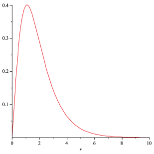
Figure 1: The gauge field strength $F_{r\,\theta}$, (2.10), in cylindrical coordinates for ${e}=\pm 1$ and $\alpha=1$.

The magnetic field (in a curved space-time) is defined as

$$B_{i} = \frac{1}{2}\sqrt{-g}\,\epsilon_{ijk}\,F^{jk}\,\,\,\,\,\,\Rightarrow\,\,\,\,\,\,$$

$$B_{z} = \frac{F_{r\,\theta}}{r}=\mp\,\frac{1}{e}\,\frac{1}{2r^{2}}\,\sqrt{\frac{2\alpha r}{\sinh\left(2\alpha r\right)}}\left[1-\frac{2\alpha r}{\tanh\left(2\alpha r\right)}\right]\,\,\,\,\,\,,$$ (2.11)

where the flat alternating tensor is such that $\epsilon_{123}=\epsilon_{r\theta z}=+1$. For completness, we have sketshed in figure (2) the function $f(r)$ and the magnetic field $B_{z}$.

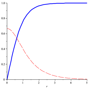
Figure 2: The thick line is the kink $f\left(r\right)=\tanh\left(\alpha\,r\right)$ while the dashed line represents the background magnetic field $B_{z}$ for ${e}=\pm 1$ and $\alpha=1$ in cylindrical coordinates.

Using the equation of motion (2.6) and the expression of $f(r)$, the energy $E$ can be written as

$$E = 2\pi\,v^{2}\int_{0}^{\infty}dr\,\left[\frac{1}{2}\partial_{r}\left(r\partial_{r}\,f^{2}\right)-\frac{\lambda}{2}\,v^{2}\,r\left(f^{4}-1\right)\right]\,\,\,\,\,\,$$ (2.12)

$$= -2\pi\,v^{2}\alpha^{2}\int_{0}^{\infty}dr\,r\left[\tanh^{4}\left(\alpha r\right)-1\right]\,\,\,\,\,\,.$$

The total derivative term does not contribute. Performing the integral we obtain

$$E=\frac{2\pi}{3}\,{v^{2}}\left[\frac{1}{2}+4\ln\left(2\right)\right]\,\,\,\,\,\,.$$ (2.13)

We recall that $E$ here is the energy per unit length.

2.2 Static solution in spherical coordinates

The same study could be repeated in spherical coordinates $x^{\mu}=\left(t\,,\,r\,,\,\theta\,,\,\varphi\right)$ for which the metric is

$$g_{\mu\nu}={\rm{diag}}\left(1\,,\,-1\,,\,-r^{2}\,,\,-r^{2}\sin^{2}\left(\theta\right)\right)\,\,\,\,\,\,.$$ (2.14)

The ansätze for the complex scalar field $\phi$ and the gauge field $A_{\mu}$ are

$$\phi = v\,f\left(r\right)\,e^{i\,n\,\theta}\,\,\,\,\,\,,$$

$$A_{\mu} = \left[0\,,\,0\,,\,-\frac{n}{e}\,,\,-\frac{1}{e}\,\sin\left(\theta\right)\,h\left(r\right)\right]\,\,\,\,\,\,.$$ (2.15)

The equation of motion is now

$$\left\{\frac{d^{2}f}{dr^{2}}-\lambda v^{2}f\left(f^{2}-1\right)\right\}+\left\{\frac{2}{r}\,\frac{df}{dr}-\frac{1}{r^{2}}fh^{2}\right\}=0\,\,\,\,\,\,.$$ (2.16)

Requiring each bracket to vanish results in

$$f\left(r\right) = \tanh\left(\alpha\,r\right)\,\,\,\,\,\,,\,\,\,\,\,\,\alpha^{2}=\frac{\lambda v^{2}}{2}\,\,\,\,\,\,,$$

$$h\left(r\right) = \pm\,{\sqrt{2}}\,\sqrt{\frac{2\alpha\,r}{\sinh\left(2\alpha\,r\right)}}\,\,\,\,\,\,.$$ (2.17)

In the case at hand, the non-vanishing components of the gauge field strength are

$$F_{r\,\varphi} = \partial_{r}\,A_{\varphi}=-\frac{1}{e}\,\sin(\theta)\frac{dh}{dr}=\mp\,\frac{1}{\sqrt{2}\,e}\,\sin(\theta)\frac{1}{r}\,\sqrt{\frac{2\alpha r}{\sinh\left(2\alpha r\right)}}\left[1-\frac{2\alpha r}{\tanh\left(2\alpha r\right)}\right]\,\,\,\,\,\,,$$

$$F_{\theta\,\varphi} = \partial_{\theta}\,A_{\varphi}=\mp\,\frac{1}{e}\cos(\theta)\,h(r)=\mp\,\frac{\sqrt{2}}{e}\cos(\theta)\,\sqrt{\frac{2\alpha r}{\sinh\left(2\alpha r\right)}}\,\,\,\,\,\,,$$ (2.18)

It can be seen that the component $F_{r\,\varphi}$ reaches a maximum for $\theta=\pi/2$ and a very small value of $r$. Away from this maximum $F_{r\,\varphi}$ tends rapidly to zero. On the other hand, $F_{\theta\,\varphi}$ has two extrema for $\theta=0$ and $\theta=\pi$ at a very small value of $r$ and goes to zero as $r$ increases.

Using the expression $B_{i}=\frac{1}{2}\sqrt{-g}\,\epsilon_{ijk}\,F^{jk}$, with $\epsilon_{r\theta\varphi}=+1$, the components of the magnetic field are

$$B_{\theta}=-F_{r\,\varphi}\,\,\,\,\,\,,\,\,\,\,\,\,B_{r}=\frac{F_{\theta\,\varphi}}{r^{2}}\,\,\,\,\,\,.$$ (2.19)

These components reach their extrema around $r=0$ and tend rapidly to zero as $r$ increases.

The corresponding energy, in the whole volume, is

$$E = \int_{0}^{2\pi}d\varphi\int_{0}^{\pi}d\theta\int_{0}^{\infty}dr\,\sqrt{-g}\,T_{00}$$ (2.20)

$$= 4\pi\,v^{2}\int_{0}^{\infty}dr\,r^{2}\left[\left(\frac{df}{dr}\right)^{2}+\frac{1}{r^{2}}\,f^{2}\,h^{2}+\frac{\lambda}{2}\,v^{2}\left(f^{2}-1\right)^{2}\right]\,\,\,\,\,\,.$$

The equation of motion (2.16) together with $f(r)=\tanh(\alpha r)$ yield

$$E = 4\pi\,v^{2}\int_{0}^{\infty}dr\,\left[\frac{1}{2}\partial_{r}\left(r^{2}\partial_{r}\,f^{2}\right)-\frac{\lambda}{2}\,v^{2}\,r^{2}\left(f^{4}-1\right)\right]\,\,\,\,\,\,$$ (2.21)

$$= -4\pi\,v^{2}\alpha^{2}\int_{0}^{\infty}dr\,r^{2}\left[\tanh^{4}\left(\alpha r\right)-1\right]\,\,\,\,\,\,.$$

The evaluation of the integral in the expression of $E$ involves the dilogarithm function ${\text{Li}}_{2}\left(z\right)$ and the final result is

$$E=\frac{4\pi}{3}\,\frac{v^{2}}{\alpha}\left(1+\frac{\pi^{2}}{3}\right)\,\,\,\,\,\,.$$ (2.22)

In reaching this result we have used the identity (see [6] for instance)

$${\text{Li}}_{2}\left(z\right)=-{\text{Li}}_{2}\left(\frac{1}{z}\right)-\frac{1}{2}\,\ln^{2}\left(-z\right)-\frac{\pi^{2}}{6}\,\,\,\,\,\,$$ (2.23)

together with the special values ${\text{Li}}_{2}\left(0\right)=0$ and ${\text{Li}}_{2}\left(-1\right)=-\pi^{2}/12$.

In conclusion, we have found simple static solutions to the equations of motion of a complex scalar field moving in a gauge field background. These are given in both cylindrical and spherical coordinates. In cylindrical coordinates, the gauge field background could be interpreted as representing a vortex located in the $(r-\theta)$ plane. This configuration of fields has a finite energy per unit length. Similarly, in spherical coordinates, the magnetic field is in the form of localised lumps in the $(r-\theta)$ and $(\theta-\varphi)$ planes. In this case, the energy available in the whole space is finite.

3 Discussion

There are various questions raised by the solutions presented in this paper. We will discuss the settings in cylindrical coordinates as this is the one relevant to the Nielsen-Olesen vortices. Let us recall briefly the situation when the gauge field $A_{\mu}$ is dynamical. In this case the theory is the full Abelian Higgs model as given by the action

$$S=\int d^{4}x\sqrt{-g}\left[-\frac{1}{4}F_{\mu\nu}F^{\mu\nu}+\left(D_{\mu}\phi\right)^{\star}\left(D^{\mu}\phi\right)-\frac{\lambda}{2}\left(\phi^{\star}\phi-v^{2}\right)^{2}\right]\,\,\,,$$ (3.1)

where $F_{\mu\nu}=\partial_{\mu}A_{\nu}-\partial_{\nu}A_{\mu}$ is the field strength of the gauge field $A_{\mu}$.

Using cylindrical coordinates together with the Nielsen-Olesen ansätze (2.5), the equations of motion of the Abelian Higgs model become

$${r}\,\frac{d}{dr}\left(\frac{1}{r}\frac{dh}{dr}\right)+2e^{2}v^{2}f^{2}\left(1-h\right) =0 \,\,\,\,\,\,,$$ (3.2)

$$\frac{1}{r}\,\frac{d}{dr}\left(r\frac{df}{dr}\right)-n^{2}\,\frac{f}{r^{2}}\left(1-h\right)^{2}-\lambda v^{2}f\left(f^{2}-1\right) =0 \,\,\,\,\,\,.$$ (3.3)

Similarly, the energy per unit length (along the $z$ direction) of the Nielsen-Olesen vortex is

$$E = 2\pi\int_{0}^{\infty}dr\,r\left[\frac{1}{r^{2}}\left(\frac{1}{2}\,\frac{n^{2}}{e^{2}}\,\left(\frac{dh}{dr}\right)^{2}+n^{2}v^{2}f^{2}\,\left(1-h\right)^{2}\right)+v^{2}\left(\frac{df}{dr}\right)^{2}+\frac{\lambda}{2}\,v^{4}\left(f^{2}-1\right)^{2}\right]$$ (3.4)

$$= 2\pi\int_{0}^{\infty}dr\,\left\{\frac{1}{4}\,\frac{n^{2}}{e^{2}}\partial_{r}\left[\frac{1}{r}\partial_{r}\left(\left(1-h\right)^{2}\right)\right]+r\left[v^{2}\left(\frac{df}{dr}\right)^{2}+\frac{\lambda}{2}\,v^{4}\left(f^{2}-1\right)^{2}\right]\right\}\,\,\,\,\,\,.$$

The above equations correspond to the minimization of $E$ with respect to both $h\left(r\right)$ and $f\left(r\right)$. The second equality is a result of the use of the equations of motion.

Since in our study the gauge field $A_{\mu}$ is taken to be a non-dynamical background, equation (3.2) was not taken into account. This raises the question of how close the expressions

$$f\left(r\right) = \tanh\left(\alpha\,r\right)\,\,\,\,,$$

$$h\left(r\right) = 1\pm\,\frac{1}{n}\sqrt{\frac{2\alpha\,r}{\sinh\left(2\alpha\,r\right)}}\,\,\,\,\,,\,\,\,\,\,\,\alpha^{2}=\frac{\lambda v^{2}}{2}\,\,\,\,\,\,$$ (3.5)

are to the solutions of the equations of motion of the Abelian Higgs model ?

Notice that for $n$ sufficiently large, the function $h\left(r\right)$ is nearly equal to $1$. Indeed, $h\left(r\right)$ is a monotonic function and varies between $1\pm\frac{1}{n}$ and $1$ for $r\in\left[0\,,\,\infty\right]$. On the other hand, $h\left(r\right)=1$ is a solution to (3.2). Therefore, as a first interpretation, we could think of the two functions $f\left(r\right)$ and $h\left(r\right)$ as approximate solutions to the equations of motion of the Abelian Higgs model for large winding number $n$.

The other feature of the study carried out in this article is that the energy in (2.13) is independent of the coupling constant $\lambda$. This leads one to think that the system is in a critical regime very much like when the Bogomolny bound is saturated at the critical coupling $\lambda=e^{2}$ and where the energy is $E=2\pi|n|v^{2}$ [7]. It is tempting to speculate that the critical regime in our analyses might correspond to the formation of an aggregate of a large number of vortices resulting in a single giant vortex.

Clusters of vortices, which are metastable, have been experimentally observed in condensed matter physics. One of the early giant vortices was observed in the superfluid Helium ⁴He with $n\approx 400$ [8]. More recently, dense arrangements of single Abrikosov vortices were detected in strongly confined superconducting condensates [9]. Giant vortices (with $n$ ranging from $7$ up to $60$) were shown to form in a rapidly rotating dilute-gas Bose-Einstein condensate [10]. It is well-known that the Abelian Higgs model (Ginzburg-Landau theory) provides the theoretical framework for these condensed matter physics phenomena. Therefore, the results presented here could be of use as far as the formation of giant vortices is concerned.

Another point regarding the solution presented in this note is that it depends very much on the expressions between the two brackets in (2.6). In other words, different assemblages of the terms are possible. The only thing that one can say about this issue is that equation (2.6) gives the general expression of the gauge field background $h(r)$ in terms of the dynamical field $f(r)$. Indeed, we have

$$\left(1-h\right)^{2}=\frac{r^{2}}{n^{2}f^{2}}\left[\frac{1}{2}\frac{1}{r}\,\frac{d}{dr}\left(r\frac{df^{2}}{dr}\right)-\left(\frac{df}{dr}\right)^{2}-\lambda v^{2}f^{2}\left(f^{2}-1\right)\right]\,\,\,\,\,\,.$$ (3.6)

The restrictions on the function $f(r)$ are then : $i)$ the expression between brackets in (3.6) is always positive and $ii)$ the energy

$$E = 2\pi\,v^{2}\int_{0}^{\infty}dr\,\left[\frac{1}{2}\partial_{r}\left(r\partial_{r}\,f^{2}\right)-\frac{\lambda}{2}\,v^{2}\,r\left(f^{4}-1\right)\right]$$ (3.7)

is finite and positive. The choice of the function $f(r)$ (satisfying the points $i)$ and $ii)$ mentioned above) is at the moment a matter of trial and error (and this is how we find our solution).

One might also want to compare the expressions (3.5) to the numerical solutions of the Abelian Higgs model. Our function $f(r)$ and the magnetic field $B_{r}$ have profiles similar to the one found using numerical analyses, as can be seen from their sketshes in figure (2).

Furthermore, we have injected the expressions of $f(r)$ and $h(r)$ given in (3.5) into the gauge field equation of motion (3.2) and evaluated this graphically. The equation of motion of the gauge field is

$$\partial_{\mu}\left(\sqrt{-g}\,F^{\mu\nu}\right)+ie\sqrt{-g}\left[\phi\left(D^{\nu}\phi\right)^{\star}-\phi^{\star}\left(D^{\nu}\phi\right)\right]$$ (3.8)

$$= -\frac{n}{e}\frac{1}{r}\left[r\frac{d}{dr}\left(\frac{1}{r}\frac{dh}{dr}\right)+2e^{2}v^{2}f^{2}\left(1-h\right)\right]=0\,\,\,\,\,.$$

Since $\left(1-h\right)$ contains a factor of $\frac{1}{n}$, the dependence on the winding number cancels and the statement made below is independent of the value of $n$.

We have first traded $r$ for the dimensionless coordinate $\rho=evr$. As a consequence, the only physical coupling constant left in (3.2) and (3.3) is $\xi=\frac{\lambda}{e^{2}}$. We then tuned $\xi$ in such a way that the graph corresponding to the left hand side of (3.2) is close to zero. Figure (3) is obtained for $\xi=4.688$.

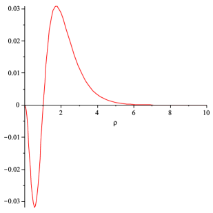
Figure 3: The gauge field equation (3.2) for $\xi=\frac{\lambda}{e^{2}}=4.688$. The horizontal axis is the rescaled coordinate $\rho=evr$.

Therefore, one could affirm that the expressions of $f(r)$ and $h(r)$ in (3.5) provide a relatively good approximate solution to the equations of motion of the Abelian Higgs model for the particular value of the coupling constant $\xi=4.688$.

Using (3.5) in (3.4), the corresponding energy is given by

$$E = \frac{2\pi}{3}\,{v^{2}}\left(\frac{\lambda}{2e^{2}}\right)+\frac{2\pi}{3}\,{v^{2}}\left[-1+4\ln\left(2\right)\right]$$ (3.9)

$$= \frac{2\pi}{3}\,{v^{2}}\left[1.344+4\ln\left(2\right)\right]\,\,\,\,\,\,.$$

This is to be compared to $E=\frac{2\pi}{3}\,{v^{2}}\left[0.5+4\ln\left(2\right)\right]$ as read from (2.13).

In summary, the expressions of $f(r)$ and $h(r)$ given in (3.5) furnish a quite good approximate solutions to the equations of motion of the Abelian Higgs model either for a large winding number or for a special value of the coupling constant $\xi=\frac{\lambda}{e^{2}}$.

Finally, we should mention that the extension of the study carried out in this paper to non-Abelian gauge theories is currently under investigation. The prototype of such theories is the $SU(2)$ Georgi-Glashow [11] model with a ’t Hooft-Polyakov ansatz [12, 13] for the gauge field $A_{\mu}^{a}$ and the scalar field $\phi^{a}$ ($a=1,2,3$). If the gauge fields are fixed backgrounds then one has only one equation of motion to solve. The whole issue is then to obtain a finite energy.

References

- [1] H. B. Nielsen and P. Olesen, Vortex-line models for dual strings, Nucl. Phys. B 61 (1973) 45-61.
- [2] Edward Witten, Superconducting strings, Nucl. Phys. B 249, Issue 4, (1985) 557-592.
- [3] Vilenkin, A., E.P.S. Shellard, Cosmic strings and other topological defects, in Cambridge Monographs in Mathematical Physics, Cambridge University Press (2000).
- [4] A. Bijl, The lowest wave function of the symmetrical many particles system, Physica, Volume 7, Issue 9, (1940) 869-886.
- [5] Robert Jastrow, Many-Body Problem with Strong Forces, Phys. Rev. 98, (1955) 1479.
- [6] Zagier D. (2007) The Dilogarithm Function. In: Cartier P., Moussa P., Julia B., Vanhove P. (eds) Frontiers in Number Theory, Physics, and Geometry II. Springer, Berlin, Heidelberg.
- [7] E. B. Bogomolny, The stability of classical solutions, Soviet Journal of Nuclear Physics, vol. 24, (1976) pp. 449–454.
-
[8]
Philip L. Marston and William M. Fairbank, Evidence of a Large Superfluid Vortex in 4He,
Phys. Rev. Lett. 39, (1977) 1208;
Erratum: Phys. Rev. Lett. 39, (1977) 1497. - [9] T. Cren, L. Serrier-Garcia, F. Debontridder and D. Roditchev, Vortex Fusion and Giant Vortex States in Confined Superconducting Condensates, Phys. Rev. Lett. 107, (2011) 097202.
- [10] P. Engels, I. Coddington, P. C. Haljan, V. Schweikhard and E. A. Cornell, Observation of Long-Lived Vortex Aggregates in Rapidly Rotating Bose-Einstein Condensates, Phys. Rev. Lett. 90, (2003) 170405.
- [11] Howard Georgi and Sheldon L. Glashow, Unified weak and electromagnetic interactions without neutral currents., Phys. Rev. Lett. 28, (1972) 1494–1497.
- [12] G. ’t Hooft, Magnetic monopoles in unified gauge theories, Nucl. Phys. B79, (1974) 276–284.
- [13] [3] A. M. Polyakov, Particle spectrum in quantum field theory, JETP Lett. 20, (1974) 194-195.