Quantum Quench and Charge Oscillations in the SU(3) Hubbard Model: a Test of Time Evolving Block Decimation with general non-Abelian Symmetries

Abstract

We introduce the notion of non-Abelian tensors, and use them to construct a general non-Abelian time evolving block decimation (NA-TEBD) scheme that uses an arbitrary number of Abelian and non-Abelian symmetries. Our approach increases the speed and memory storage efficiency of matrix product state based computations by several orders of magnitudes, and makes large bond dimensions accessible even on simple desktop architectures. We use it to study post-quench dynamics in the repulsive SU(3) Hubbard model, and to determine the time evolution of various local operators and correlation functions efficiently. Interactions turn algebraic charge relaxation into exponential, and suppress coherent quantum oscillations rapidly.

I Introduction

Matrix product state based numerical renormalization approaches such as Wilson’s original numerical renormalization group (NRG) method Krishna-murthy et al. (1980a, b) or the density matrix renormalization group (DMRG) introduced by Steven R. White,White (1992); Schollwöck (2005, 2011) proved to be extremely powerful tools to study low-energy properties of strongly interacting many-body systems.

Though the original methods were designed to address the ground state properties of zero and one dimensional quantum systems, modern offsprings of NRG and DMRG earned wide applications: the time-evolving block decimation (TEBD) algorithm,Vidal (2004, 2007a) time dependent DMRG,White and Feiguin (2004) or the time dependent variational principle (TDVP) algorithms Haegeman et al. (2011) allow one to study the evolution of closed quantum systems in real or imaginary time, while in two dimensions, the projected entangled paired states (PEPS) approach Verstraete et al. (2008); Orús (2014) has been proposed as a viable extension of MPS states. For Gapless models Multiscale Entanglement Renormalization Ansatz (MERA) is a suitable choice,Vidal (2007b) while tree tensor network states (TTNS) represent another promising direction for models with long-ranged interactions. Gunst et al. (2018); Nakatani and Chan (2013)

DMRG, however, continues to be a very attractive and robust approach for systems with long-ranged interactions as well as for one- and two-dimensional systems, (see, e.g., Ref. Szalay et al., 2015), and provides a valid alternative to more sophisticated approaches, which often display less favorable computational scaling with the so-called bond dimension.Lubasch et al. (2014); Corboz (2016)

Exploiting the symmetry of the problem as much as one can is always a crucial ingredient in numerical simulations: it reduces the computational cost and boosts up the accuracy. It is straightforward to implement Abelian symmetries, such as parity or charge conservation in most MPS and tensor network algorithms.iTE ; Bauer et al. (2011) Handling non-Abelian symmetries is, however, much more challenging. It has been known for a long time how to treat non-Abelian symmetries in NRG Krishna-murthy et al. (1980a, b); Tóth et al. (2008); Moca et al. (2012) and DMRGMcCulloch and Gulácsi (2002) simulations, and $SU(2)$ symmetry has also been implemented in TEBD,Singh et al. (2010) in TTNS,Gunst et al. (2019) and in PEPS,Hubig (2018) yet a unified non-Abelian tensor framework incorporating non-Abelian symmetries remained a challenge.

Figure 1: Graphical representation of an NA-tensor $T(\left\{\Gamma\right\})_{i_{1}\,i_{2}\dots i_{n}}^{j_{1}\,j_{2}\dots j_{m}}$. Incoming and outgoing legs correspond to lower and upper indices. Tensor blocks are labeled by the representation indices $\left\{\Gamma\right\}=(\Gamma_{1},\dots,\Gamma_{k})$.

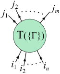
In Ref. Werner et al., 2019, we introduced the general structure of non-Abelian tensors (NA-tensors), which provides the requested unified framework, and applied this approach to describe the time evolution of the $S=1$ Heisenberg chain and to study quasiparticle dynamics. NA-tensors, depicted in Fig.1, are objects that carry symmetry labels (representation labels) as internal arguments, and have external legs, which, however, may be tied to the aforementioned internal symmetry labels. Line directions indicate regular or conjugate representations. We remark that our NA-tensors resemble the previously introduced Q-spaces tensor class,Weichselbaum (2012, 2020) but the treatment of symmetry dependent parts of the tensor networks is substantially and conceptually different in our construction. The structure we introduce here encodes in a natural way non-Abelian MPS structures, Clebsch-Gordan coefficients, 6J and 9J symbols,Wigner (1959) and provides a technically transparent framework to handle non-Abelian symmetries, in general.

In this work, we give a detailed account of this mathematical and computational framework, and demonstrate its performance on an experimentally relevant system, the fermionic SU(3) Hubbard model,

$$\hat{H}=-J\sum_{\alpha}\sum_{l=1}^{L-1}\big{(}c^{\dagger}_{l,\alpha}c_{l+1,\alpha}+h.c.\big{)}+U\sum_{l=1}^{L}\sum_{\alpha\neq\alpha^{\prime}}n_{l,\alpha}n_{l,\alpha^{\prime}}\,.$$ (1)

Here $J$ denotes the hopping amplitude between nearest-neighbors sites, $U$ represents the local strength of the interaction and $n_{i,\alpha}$ is the number operator at a given site, $n_{i,\alpha}=c^{\dagger}_{i,\alpha}c_{i,\alpha}$. This model displays an overall $\text{SU(3)}\times\text{U(1)}$ symmetry, which we use to obtain a compact NA-MPS description of the time evolution. In the following, if not explicitly displayed, energies and time are measured in units of $J$ and $J^{-1}$, respectively.

The one-dimensional model, Eq. (1) is not just of pure theoretical interest. Both its attractive Hofstetter et al. (2002) and its repulsive versions Boll et al. (2016) have been realized by ultracold atoms trapped in optical lattices, where the real-time dynamics can be carefully observed. Here we study the SU(3) version of the experiment realized in Ref Trotzky et al., 2012 with ${}^{87}\mathrm{Rb}$ atoms: we prepare an initial state with groups of three atoms placed on every third site (see Fig.2). As we demonstrate, in the absence of interactions charge oscillations relax to the average occupation algebraically, and long-ranged spatial correlations develop. A finite interaction strength changes this behavior dramatically, rapidly suppresses coherent charge oscillations, and induces exponential charge equilibration.

The paper is structured as follows: We introduce non-Abelian matrix product states in Section II. Non-Abelian tensors (NA-tensors) and their algebraic properties are presented in Section III. We describe the generalized non-Abelian TEBD algorithm in Section IV, while results for various quantities such as the charge oscillation or the entanglement entropy growth in the SU(3) Hubbard model are presented in Section V. We benchmark the efficiency of our code In Section VI, and summarize our results and conclusions in Section VII. Certain technical details have been relegated to appendices.

Figure 2: Initial state of the SU(3) Hubbard chain. Fermions sit in groups of 3 on every third site of the optical lattice.

II Non-Abelian Matrix Product States

II.1 MPS representation of quantum states

The MPS representation of a state $\left|\Psi\right\rangle$ can be written asSchollwöck (2011); Orús (2014)

$$\left|\Psi\right\rangle = \sum_{a_{1},\dots a_{L-1}}\sum_{\sigma_{1},\dots\sigma_{L}}\mathcal{A}^{[1]\,a_{1}}_{\sigma_{1}}\mathcal{A}^{[2]\,a_{2}}_{a_{1}\sigma_{2}}\dots\mathcal{A}^{[L]}_{a_{L-1}\sigma_{L}}\times$$ (2)

$$\left|\sigma_{1}\right\rangle\otimes\left|\sigma_{2}\right\rangle\otimes\dots\otimes\left|\sigma_{L}\right\rangle\;.$$

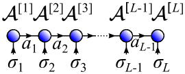
Here the states $\left|\sigma_{l}\right\rangle$ span the local Hilbert space $\mathcal{H}_{l}$ at site $l$. In case of the SU(3) Hubbard chain, e.g., each site has $2^{3}=8$ states. Representation Eq. (2) possesses an enormous gauge freedom, and the ’matrices’ $\mathcal{A}^{[l]}$ are not uniquely defined. In the following, we use the so-called ’left-canonical’ MPS representation, where the MPS is obtained by using the left Schmidt states of the so-called Schmidt decomposition.Schollwöck (2011); Orús (2014); Schmidt (2907) To achieve this, we cut the system into two parts at bond $l$, and perform a Schmidt decomposition with this partitioning to yield

$$\left|\Psi\right\rangle\to\sum_{a}\lambda^{[l]}_{a}\,\left|a\right\rangle_{l}\otimes\left|\bar{a}\right\rangle_{l}\;.$$ (3)

Here $\left|a\right\rangle_{l}$ and $\left|\bar{a}\right\rangle_{l}$ refer to the left and right orthonormal Schmidt states, respectively. Making a cut at the bond $l+1$ yields a similar decomposition with another set of left Schmidt states, $\left|a\right\rangle_{l+1}$. These latter can, however, also be built up from the states $\left|a\right\rangle_{l}$ and the local states $\left|\sigma\right\rangle_{l+1}$ at site $l+1$, as

$$\left|a^{\prime}\right\rangle_{l+1}=\sum_{a,\sigma}\big{(}\mathcal{A}^{[l+1]}\big{)}^{a^{\prime}}_{a\sigma}\left|a\right\rangle_{l}\otimes\left|\sigma\right\rangle_{l+1}\;.$$ (4)

Iterating this equation leads to the MPS representation, Eq. (2). Due to the orthogonality of Schmidt states the $\mathcal{A}$’s satisfy the ’half-unitary’ conditions,

$$\sum_{\sigma,a}\mathcal{A}_{\phantom{ab}a\,\sigma}^{[l]\,a^{\prime}}\left(\mathcal{A}_{\phantom{ab}a\,\sigma}^{[l]\,a^{\prime}}\right)^{*}=\delta_{a^{\prime}}^{a^{\prime}}\;.$$ (5)

One can similarly introduce ’right-canonical’ MPS based on the right Schmidt states $\left|\bar{a}\right\rangle_{l}$, however, since TEBD can be formulated purely in terms of left-canonical matrices, we do not discuss them here.

Notice that the ’matrices’ $\mathcal{A}^{[l]}$ are rather tensors than matrices, since they have three indices. The two ’incoming’ states $\left|a\right\rangle_{l}$ and $\left|\sigma\right\rangle_{l}$ in Eq. 4 appear as lower indices, while the ’outgoing’ state $\left|a^{\prime}\right\rangle_{l+1}$ is displayed as an upper index. This leads us to the pictorial representation in Fig. 3. It is useful to associate incoming arrows with lower (’ket’) indices, and outgoing arrows with upper (’bra’) indices. The aforementioned gauge symmetry implies namely that incoming legs can only be contracted with ’outgoing’ ones.

Figure 3: Left-canonical MPS tensor diagram corresponding to Eq. (2).

II.2 Locally generated global symmetries for lattice models

Generic Hamiltonians display various symmetries, which help us to organize states. Here we consider symmetries with unitary representations, where each element $g$ of a symmetry group $\mathcal{G}$ corresponda to some unitary operator, $\hat{U}(g)$, which commutes with the Hamiltonian,

$$\left[\hat{H},\hat{\mathcal{U}}(g)\right]=0\,,\quad\forall g\in\mathcal{G}\;.$$ (6)

Eigenstates of the Hamiltonian can then be labeled by the irreducible representations (’quantum numbers’) of the group $\mathcal{G}$, and can thus be organized into multiplets,

$$\mathcal{H}=\mathrm{span}\left\{\left|\Gamma;t_{\Gamma},m_{\Gamma}\right\rangle\right\}\;.$$ (7)

Here we have grouped states into ’sectors’ according to to the representation index $\Gamma$. Within each sector $\Gamma$, $t_{\Gamma}$ labels the multiplets, while $m_{\Gamma}$ is a symmetry-related internal quantum number. States within a multiplet $(\Gamma;t_{\Gamma})$ are transformed among each other under the action of the $\hat{\mathcal{U}}(g)$’s, and are degenerate.

For multiple symmetries, that is $\mathcal{G}=\mathcal{G}_{1}\otimes\dots\otimes\mathcal{G}_{n_{S}}$, representation indices form a list $\Gamma=(\Gamma_{1},\dots,\Gamma_{n_{S}})$. In case of the SU(3) Hubbard model, discussed here, the global symmetry is SU(3) $\times$U(1), and, accordingly, multiplets will be labeled by SU(3) representations and U(1) charges (i.e., particle number).

Here we restrict ourselves to locally generated global symmetries, for which $\hat{\mathcal{U}}(g)$ factorizes as

$$\hat{\mathcal{U}}(g)=\hat{\mathcal{U}}_{1}(g)\otimes\hat{\mathcal{U}}_{2}(g)\otimes\dots\otimes\hat{\mathcal{U}}_{L}(g)\,,$$ (8)

with the $\hat{\mathcal{U}}_{i}(g)$’s operating only at site $i$. In this case , the local Hilbert space at each lattice site $i$ can also be organized into multiplets (sectors),

$$\mathcal{H}_{i}=\mathrm{span}\left\{\left|\Gamma^{\mathrm{loc}};\tau_{\Gamma^{\mathrm{loc}}},\mu_{\Gamma^{\mathrm{loc}}}\right\rangle_{i}\right\}\;,$$ (9)

with the $\Gamma^{\mathrm{loc}}$ labeling local representations, $\tau_{\Gamma^{\mathrm{loc}}}$ denoting the associated local multiplets, and $\mu_{\Gamma^{\mathrm{loc}}}$ the internal index of the given representation.

Hereinafter, for clarity, multiplet and internal labels associated with a single site shall be denoted by greek letters, while states or multiplets for multi-site (sub) systems are denoted by latin letters.

II.3 Non-belian MPS: matrix product states with non-Abelian symmetries

The easiest way to obtain the non-Abelian MPS (NA-MPS) representation of a state $\left|\Psi\right\rangle$ is to exploit Schmidt decomposition introduced in Subsection II.1. The construction in Eqs. (3) and (4) carries over in the presence of non-Abelian symmetries, too. The only modification is that Schmidt states are now grouped into multiplets, $\left|a\right\rangle\to\left|\Gamma;t_{\Gamma},m_{\Gamma}\right\rangle$, and Schmidt states constructed on neighboring bonds $l$ and $l+1$ are related via the Clebsch-Gordan coefficients of the symmetry group $\mathcal{G}$,

$$\left|\Gamma^{\prime};t_{\Gamma^{\prime}},m_{\Gamma^{\prime}}\right\rangle_{l+1}= \sum_{\Gamma,\Gamma^{\mathrm{loc}}}\;\sum_{t_{\Gamma},\tau_{\Gamma^{\mathrm{loc}}}}\;\sum_{\alpha_{\{\Gamma\}}}A^{[l+1]}(\Gamma,\Gamma^{\mathrm{loc}},\Gamma^{\prime})_{t_{\Gamma}\,\tau_{\Gamma^{\mathrm{loc}}}\,\alpha_{\{\Gamma\}}}^{t_{\Gamma^{\prime}}}\times$$ (10)

$$\sum_{m_{\Gamma},\mu_{\Gamma^{\mathrm{loc}}}}C(\Gamma,\Gamma^{\mathrm{loc}},\Gamma^{\prime})_{m_{\Gamma}\,\mu_{\Gamma^{\mathrm{loc}}}}^{m_{\Gamma^{\prime}}\,\alpha_{\{\Gamma\}}}\left|\Gamma;t_{\Gamma},m_{\Gamma}\right\rangle_{l}\otimes\left|\Gamma^{\mathrm{loc}};\tau_{\Gamma^{\mathrm{loc}}},\mu_{\Gamma^{\mathrm{loc}}}\right\rangle_{l+1}\;.$$

Here, to emphasize their tensor character, the usual Clebsch-Gordan coefficients have been denoted in a somewhat unusual way, $\left(\Gamma,m_{\Gamma};\Gamma^{\mathrm{loc}},\mu_{\Gamma^{\mathrm{loc}}}|\Gamma^{\prime},m_{\Gamma^{\prime}}\right)_{\alpha_{\{\Gamma\}}}\to C(\Gamma,\Gamma^{\mathrm{loc}},\Gamma^{\prime})_{m_{\Gamma}\,\mu_{\Gamma^{\mathrm{loc}}}}^{m_{\Gamma^{\prime}}\,\alpha_{\{\Gamma\}}}$, with $\alpha$ the so-called outer multiplicity label.Cornwell (1984) This label is usually introduced for more complex groups such as SU($n>2$) or cubic symmetries, e.g., where certain irreducible representations occur multiple times in the product of two other representations. The outer multiplicity label is usually dropped for symmetries such as O(3) or SU(2), but it proves extremely useful to keep it even in these simple cases. The interpretation of Eq.  (10) is simple: we use Clebsch-Gordan coefficients to construct the multiplets $\Gamma^{\prime}$ from representations $\Gamma$ and $\Gamma^{\mathrm{loc}}$, and then mix these with the NA-tensor $A(\Gamma,\Gamma^{\mathrm{loc}},\Gamma^{\prime})$ to obtain the appropriate Schmidt state. In the construction above, we have tacitly assumed that the state $\left|\Psi\right\rangle$ is a ’singlet’, i.e., that it transforms according to the trivial representation, $\Gamma=0$. Then the trivial symmetry structure of $\left|\Psi\right\rangle$ ensures that Schmidt-states form multiplets. The construction can, however, be easily generalized to the case $\Gamma\neq 0$ (see Appendix A for details).

Figure 4: Adding a site to the left subsystem. (a) Schmidt states of the new, ’larger’ subsystem form multiplets classified by the irreducible representations ($\Gamma^{\prime}$). (b) Corresponding tensor diagram, representing Eqs. (11) and (12). Contracting the label $\alpha$ yields a standard MPS representation, Eq. (2), which does not exploit symmetries.

We pose here for a moment to investigate the structure of the tensors appearing in the construction above. The Clebsch-Gordan coefficient and the matrix $A$ are both four-leg tensors, ogranized into blocks according to the three representation labels, $\{\Gamma\}=(\Gamma,\Gamma^{\mathrm{loc}},\Gamma^{\prime})$. The external legs of these tensors are, however, tied to the block’s considered. Certain legs, such as the $t$’s, $\tau$, the $m$’s and $\mu$, depend only on a particular representation, which we displayed as a label. The outer multiplicity label $\alpha$, however, depends on all three $\Gamma$’s. These dependencies play a crucial role in what follows: as we shall see, only tensor legs with identical dependencies can be contracted. This is already clear in Eq.  (10), where summation over the multiplicity label $\alpha$ enforces the symmetry labels of $A^{[l]}$ and $C$ to be identical.

Eq. (10) is graphically represented in Fig. 4. We can rewrite Eq. (10) by simply suppressing the (quite obvious) dependency of the legs as

$$\left|\Gamma^{\prime};t^{\prime},m^{\prime}\right\rangle_{l+1}=\sum_{\Gamma,\Gamma^{\mathrm{loc}}}\;\sum_{t,\tau}\;\sum_{\alpha}A^{[l+1]}(\{\Gamma\})_{t\,\tau\,\alpha}^{t^{\prime}}\sum_{m,\mu}C(\{\Gamma\})_{m\,\mu}^{m^{\prime}\,\alpha}\left|\Gamma;t,m\right\rangle_{l}\otimes\left|\Gamma^{\mathrm{loc}};\tau,\mu\right\rangle_{l+1}\;$$ (11)

The direct relationship between Eq. (11) and (4) can be established by summing over the outer multiplicity label $\alpha$ (see also Fig. 4.b),

$$\sum_{\alpha}A^{[l+1]}(\left\{\Gamma\right\})_{t\,\tau\,\alpha}^{t^{\prime}}C(\left\{\Gamma\right\})_{m\,\mu}^{m^{\prime}\,\alpha}=\mathcal{A}^{[l+1]}(\{\Gamma\})_{t\,m\;\;\tau\,\mu}^{t^{\prime}\,m^{\prime}}\;.$$ (12)

Iterating Eq. (11), we arrive at the left-canonical NA-MPS representation of the state $\left|\Psi\right\rangle$,

$$\left|\Psi\right\rangle=\sum_{\left\{\Gamma^{\mathrm{loc}}_{l}\right\}}\sum_{\left\{\Gamma_{l}\right\}}\sum_{\left\{t_{l}\right\}}\sum_{\left\{\tau_{l}\right\}}\;\sum_{\left\{\alpha_{l}\right\}} A^{[1]}(\left\{\Gamma\right\}^{[1]})_{\tau_{1}\,\alpha_{1}}^{t_{1}}\,A^{[2]}(\left\{\Gamma\right\}^{[2]})_{t_{1}\,\tau_{2}\,\alpha_{2}}^{t_{2}}\,\dots\,A^{[L]}(\left\{\Gamma\right\}^{[L]})_{t_{L-1}\,\tau_{L}\,\alpha_{L}}$$

$$\sum_{\left\{m_{l}\right\}}\sum_{\left\{\mu_{l}\right\}} C(\left\{\Gamma\right\}^{[1]})_{0\,\mu_{1}}^{m_{1}\,\alpha_{1}}\,C(\left\{\Gamma\right\}^{[2]})_{m_{1}\,\mu_{2}}^{m_{2}\,\alpha_{2}}\,\dots\,C(\left\{\Gamma\right\}^{[L]})_{m_{L-1}\,\mu_{L}}^{0\,\alpha_{L}}$$ (13)

$$\left|\Gamma^{\mathrm{loc}}_{1};\tau_{1},\mu_{1}\right\rangle\otimes\left|\Gamma^{\mathrm{loc}}_{2};\tau_{2},\mu_{2}\right\rangle\otimes\dots\otimes\left|\Gamma^{\mathrm{loc}}_{L};\tau_{L},\mu_{L}\right\rangle\;,$$

where we have added a site label $l$ to the general notation $(\Gamma_{l-1},\Gamma^{\mathrm{loc}}_{l},\Gamma_{l})\to\left\{\Gamma\right\}^{[l]}$, with $\Gamma_{l}$ denoting the representation indices of Schmidt states on the left of bond $l$. The formally introduced representation index $\Gamma_{0}=0$ stands for the ’empty’ site, $l=0$, while $\Gamma_{L}=0$ is just the trivial representation to which the state $\left|\Psi\right\rangle$ belongs. (Generalization to $\Gamma_{L}\neq 0$ states is discussed in Appendix A.)

Figure 5: Representation of the NA-MPS in equation (II.3). Multiplet indices $t_{l},\tau_{l}$ and the outer multiplicity indices $\alpha_{l}$ are shown in black, while internal $\mu_{l},m_{l}$ indices of the representations are marked by orange. The upper layer is free from internal indices of representations, but has a block structure, as classified by the representation labels $\{\Gamma\}$. Clebsch-Gordan coefficients form the lower layer.

Fig. 5 shows a graphical representation for the NA-MPS state in Eq. (II.3). It is constructed as a two layer structure, with the lower layer containing symmetry/representation-specific information, encoded through Clebsch-Gordan coefficients. The upper layer has, of course, also some knowledge about the underlying symmetry, since its blocks are labeled by the irreducible representations, but does not contain representation-specific information. This two-layer structure is somewhat similar to those in the SU(2) symmetric implementations presented in Refs. Singh et al., 2010; Gunst et al., 2019. Here, however, we take also keep track of outer multiplicities in a very general way, which allows us to treat symmetries beyond SU(2) in a unified, transparent, and symmetry group independent manner.

Our goal is to eliminate the lower layer, and perform DMRG or TEBD only on the upper layer, which can thus be considered as a full-fledged representation of the state $\left|\Psi\right\rangle$. Removing the Clebsch layer improves efficiency in two ways: i) Since bond indices $t_{l}$ in the upper layer stand for multiplets instead of states, the bond dimension $M_{\mathrm{mult}}$ of the upper layer corresponds to a much larger conventional (’non symmetric’) bond dimension. ii) The representation indices $\left\{\Gamma\right\}^{[l]}$ must respect symmetry-specific selection rules. These selection rules allow for a very efficient sparse block storage, tensor multiplication, and singular value decomposition (SVD).Roy and Banerjee (2014)

Although we refer to the tensor structure introduced as non-Abelian, it naturally incorporates familiar Abelian symmetries, too. For Abelian symmetries such $U(1)$ or parity (${\cal Z}_{2}$), e.g., all representations are one-dimensional, all ’Clebsches’ are just ones for blocks allowed by the selection rules, and the regular MPS structure is recovered with efficient sparse block tensors in the decomposition.

III NA-tensors

III.0.1 NA-tensors and dependencies

The tensors $A^{[l]}$, and the Clebsch-Gordan coefficients $C$ in Eqs. (11) and (II.3), have the same fundamental structure, which we refer to as non-Abelian tensor (NA-tensor). General NA-tensors $T(\left\{\Gamma\right\})_{i_{1}\,i_{2}\dots i_{n}}^{j_{1}\,j_{2}\dots j_{m}}$, have a structure shown in Fig. 1: they have a block structure with blocks labeled by lists of symmetry labels (representation indices), $\left\{\Gamma\right\}=(\Gamma_{1},\dots,\Gamma_{k})$, with each $\Gamma_{i}$ referring to a list of quantum numbers used. They have, furthermore, external incoming and outgoing legs. Since many blocks contain only zeros by selection rules, an efficient sparse block storage can be achieved by storing only non-zero blocks. Block sizes usually depend on the specific set of representations $\left\{\Gamma\right\}$, and can have different block sizes at every site.

The legs of NA-tensors have implicit dependence on the tensor’s internal symmetry labels. The label $t$ in Eq. (11), e.g., runs over multiplets belonging to a given representation, $\Gamma$. Similarly, the index $m$ can take $\dim(\Gamma)$ different values. Thus both $t$ and $m$ depend on the representation index $\Gamma$. The outer multiplicity index $\alpha$ depends on all three representation indices labeling a given (non-vanishing) symmetry block of the Clebsch-Gordan tensor, as well as that of the tensor $A^{[l]}$. Generally, any given leg of an NA-tensor depends on a given subset of the representations $\left\{\Gamma\right\}$, labeling the blocks.

III.0.2 Multiplication rules

The MPS representation in Eq. (II.3) (see also Fig. 5) allows us to introduce multiplication rules. By construction, the tensors $A^{[l]}$ and $C$ belonging to the same site are glued together such that the three representation indices $\left\{\Gamma\right\}^{[l]}=(\Gamma_{l-1},\Gamma^{\mathrm{loc}}_{l},\Gamma_{l})$ are always the same. This is, in fact, enforced by the contraction of the outer-multiplicity index $\alpha$. Similarly, we may notice that only those tensor blocks of $A^{[l]}$ and $A^{[l+1]}$ are contracted through the index $t_{l}$, where the corresponding representation $\Gamma_{l}$ (associated with the bond between sites $l$ and $l+1$) is identical. Similar observations can be made by investigating the Clebsch-Gordan tensors.

These observations lead us to the general (graphical) contraction rule:

1. Incoming legs of NA-tensors can be contracted with outgoing legs provided that all their dependencies match.

2. The resulting tensor’s blocks are labeled by the representation tensor indices of the original tensors, but the matched representation indices are listed only once.

In large tensor networks, such as the ones displayed in in Figs. 14 and 15, virtually all legs are contracted, but the rules above would result in NA-tensors whose blocks are still labeled by all representation indices $\Gamma^{\mathrm{loc}}_{l}$ and $\Gamma_{l}$, while most of the representation indices are redundant in the sense that remaining legs do not depend on them. Note also that Eq. (II.3) contains a summation over representations index sets, $\left\{\Gamma_{l}\right\}$ and $\left\{\Gamma^{\mathrm{loc}}_{l}\right\}$. It is therefore useful to introduce the following rule,

1. If there is one or more representation indices in the result tensor that no remaining (uncontracted) legs depend on, then blocks must be summed over these representation indices.

This rule eliminates redundant representation indices.

At the end of this section, let us compare our NA-tensors with the ’QSpaces’ tensors introduced by Andreas Weichselbaum.Weichselbaum (2012, 2020) The main difference between the two approaches is the handling of Clebsch-Gordan coefficients. In Ref. Weichselbaum, 2012 tensors are more complicated objects: they have not just blocks, but every block consists of more layers: one layer contains the representation-independent parts of the tensor (this layer correspond to our $A^{[l]}$ tensors), while other layers contain the Clebsch-Gordan coefficients (or their various combinations) for different symmetries. In these abstract tensors structural and Clebsch-Gordan blocks are grouped together for every enabled set of representation labels. This multilayer structure leads to sophisticated multiplication rules.Weichselbaum (2020) In contrast, in our approach we separate completely the Clebsch-Gordan coefficients from the structural $A^{[l]}$ tensors, and collect them into the $C$ tensor, whose mathematical structure is essentially the same as that of the $A^{[l]}$ tensors. As a result, our NA-tensors are conceptually simpler objects with relatively simple multiplication rules.

IV Time evolving block decimation with NA-tensors

IV.1 Basic steps of TEBD

We now demonstrate the NA-MPS approach on one of the simplest MPS algorithms, the time evolving block decimation (TEBD). This method, originally introduced by Guifré Vidal,Vidal (2004, 2007a) has since been exhaustively used to simulate one dimensional quantum systems in out of equilibrium.Žnidarič et al. (2008); Bardarson et al. (2012); Pozsgay et al. (2014); Schreiber et al. (2015); Else et al. (2016) We consider here Hamiltonians with nearest neighbor interactions,

$$\hat{H}=\sum_{i=1}^{L-1}\hat{h}^{(2)}_{i,i+1}\;,$$ (14)

with $\hat{h}^{(2)}_{i,i+1}$ acting on sites $i$ and $i+1$. Within TEBD, one divides $\hat{H}$ into parts acting on even and odd bonds,

$$\hat{H}=\hat{H}_{\mathrm{even}}+\hat{H}_{\mathrm{odd}}=\sum_{k}\hat{h}^{(2)}_{2k,2k+1}+\sum_{k}\hat{h}^{(2)}_{2k+1,2k+2}\;,$$ (15)

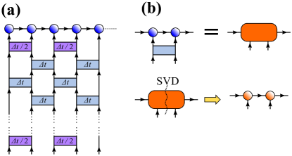
and ’Trotterizes’ the time evolution operator $e^{-i\hat{H}t}$, i.e., divides time into small segments of length $\Delta t$, and then applies a second order Trotter-Suzuki approximation Trotter (1959); Suzuki (1976), $e^{-i\Delta t\hat{H}}\approx e^{-i\Delta t\,\hat{H}_{\mathrm{even}}/2}e^{-i\Delta t\,\hat{H}_{\mathrm{odd}}}e^{-i\Delta t\,\hat{H}_{\mathrm{even}}/2}$. This procedure yields the time evolution, represented in Fig. 6. Time evolution occurs on bonds, and after each step, singular value decomposition (SVD) can be used to reconstruct the original MPS structure of the state $\left|\Psi(t)\right\rangle$.

Figure 6: (a) Time evolution with second order Trotter-Suzuki approximation, yielding a sequence of two-site operations, generated by the even and odd bond parts of the Hamiltonian. (b) SVD is used after each step to restore the original MPS structure.

IV.2 TEBD with NA-MPS

Figure 7: (a) Matrix element of the time evolution operator between two NA-MPSs. (b-c) Almost all Clebsch-Gordan tensors can be eliminated using orthogonality relations, leading to a reduced time evolution operator. (d) The reduced tensors $U_{\mathrm{red}}$ act then directly on the top layer of the NA-MPS.

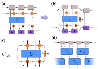
We now extend TEBD to non-Abelian MPS’s to obtain the non-Abelian version of TEBD (NA-TEBD). Here we focus on the key steps and use a graphical language (see Fig. 7). Technical details are relegated to Appendices B and D.

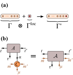
The crucial step is the construction of a reduced evolution operator $U_{\mathrm{red}}$, which incorporates unnecessary Clebsch-Gordon coefficients, and time evolves only the upper layer of the NA-MPS state. The overall construction of the $U_{\mathrm{red}}$ is presented in Fig. 7. To obtain $U_{\mathrm{red}}$, we compute the overlap $\left\langle\tilde{\Psi}\right|U\left|\Psi\right\rangle$, with both states being written in the NA-MPS form (such an overlap is graphically displayed in panel (a) in Fig. 7). Using the orthogonality properties of ’Clebsches’ (see Appendix B), we can eliminate all but four Clebsch-Gordan tensors, which are then incorporated into the reduced evolution operator (panel (b) in Fig. 7). This leaves us with the reduced two-site propagator, $U_{\mathrm{red}}(\left\{\Gamma\right\})_{\tau_{l}^{\prime}\,\alpha_{l}^{\prime}\;\;\tau_{l+1}^{\prime}\,\alpha_{l+1}^{\prime}}^{\tau_{l}\,\alpha_{l}\;\;\tau_{l+1}\,\alpha_{l+1}}$, acting on sites $l$ and $l+1$ (panel (c) in Fig. 7).

Notice that this eight-leg NA-tensor is labeled by a total of eight representation indices: $\left\{\Gamma\right\}=\left(\Gamma_{l-1},\Gamma_{l}^{\mathrm{loc}},{\Gamma_{l}^{\mathrm{loc}}}^{\prime},\Gamma_{l},\Gamma_{l}^{\prime},\Gamma_{l+1}^{\mathrm{loc}},{\Gamma_{l+1}^{\mathrm{loc}}}^{\prime},\Gamma_{l+1}\right)$. The indices $\tau$ depend just on local representations, while the dependencies of the outer multiplicities $\alpha$ read $\mathrm{dep}(\alpha_{l})=(\Gamma_{l-1},\Gamma_{l}^{\mathrm{loc}},\Gamma_{l})$, $\mathrm{dep}(\alpha_{l+1})=(\Gamma_{l},\Gamma_{l+1}^{\mathrm{loc}},\Gamma_{l+1})$ , $\mathrm{dep}(\alpha_{l}^{\prime})=(\Gamma_{l-1},{\Gamma_{l}^{\mathrm{loc}}}^{\prime},\Gamma_{l}^{\prime})$, and $\mathrm{dep}(\alpha_{l+1}^{\prime})=(\Gamma_{l}^{\prime},{\Gamma_{l+1}^{\mathrm{loc}}}^{\prime},\Gamma_{l+1})$. Notice that, numerically, it is sufficient to compute the reduced evolution operator $U_{\mathrm{red}}$ only once.

Having discarded the Clebsch-layer, the reduced operator now acts only on the upper layer of the $A^{[l]}$-tensors. From now on, there is no significant difference between the NA-TEBD and the usual TEBD; the upper layer of NA-MPS behaves in the simulations like a normal MPS that is updated at each time step, only the singular value decomposition step, discussed in more detail in Appendix D requires some care (see also Fig. 7 (d)).

Since NA-TEBD is formulated in terms of the upper layer of the NA-MPS, one does not need to take care of internal states of multiplets, and necessary numerical resources are determined by the bond dimension of the upper layer, $M_{\mathrm{mult}}$. Due to the block structure of the $A^{[l]}$-tensors, the SVD transformation can be performed separately according to the representation indices of the Schmidt states. In this way, we can reach bond dimensions in the range of tens of thousands in terms of usual, non-symmetric or Abelian states even on simple desktop computers.

V Application to the SU(3) Hubbard model

We now illustrate the advantages of NA-TEBD by simulating a quantum quench on the one dimensional Hubbard model, Eq. (1), at $1\over 3$-filling.

In this case, the local Hilbert space is $d=2^{3}=8$ dimensional. The model defined by Eq. (1) possesses a U(1) charge symmetry, generated by the total charge,

$$\hat{Q}\equiv\sum_{l}\;\hat{q}_{l}\,,\quad\quad\mbox{with}\quad\hat{q}_{l}=\sum_{\alpha}(c^{\dagger}_{l,\alpha}c_{l,\alpha}-1/2)\;,$$

and an SU(3) symmetry generated by the eight SU(3) generators,

$$\hat{\Lambda}^{i}\equiv\sum_{l}\;{\hat{\lambda}}^{i}_{l}\;,\quad\quad\mbox{with}\quad\hat{\lambda}^{i}_{l}=\sum_{\alpha,\beta}c^{\dagger}_{l,\alpha}\lambda^{i}_{\alpha\beta}c_{l,\beta}\;.$$

Here the $\lambda^{i}$ denote the usual Gell-Mann matrices, satisfying the SU(3) Lie algebra, $[\lambda^{i},\lambda^{j}]=if^{ijk}\lambda^{k}$. The Hamiltonian commutes with all generators above, and has a corresponding $\mbox{SU(3)}\times\mbox{U(1)}$ symmetry.

The local Hilbert space at each site is spanned by four multiplets, organized according to the total charge $Q^{\mathrm{loc}}$ and an $SU(3)$ representation label, typically specified by a Young tableau (see Table 1). In case of SU(3), possible Young tableaux consist if two lines, and the length of these lines $F\equiv(m_{1},m_{2})$ specify the representation. The local representation label is therefore a composite label, $\Gamma^{\mathrm{loc}}_{l}=\{F^{\mathrm{loc}},Q^{\mathrm{loc}}\}$.

$\Gamma^{\mathrm{loc}}=(F^{\mathrm{loc}},\;Q^{\mathrm{loc}})$	$\dim(\Gamma^{\mathrm{loc}})$	$\dim(\tau)$	states
(•,  0 )	1	1	$\left|0\right\rangle$
			$c^{\dagger}_{1}\left|0\right\rangle$
( ${\yng(1)}$ ; 1)	3	1	$c^{\dagger}_{2}\left|0\right\rangle$
			$c^{\dagger}_{3}\left|0\right\rangle$
			$c^{\dagger}_{1}c^{\dagger}_{2}\left|0\right\rangle$
$\Big{(}\,\yng(1,1)\,;2\Big{)}$	3	1	$c^{\dagger}_{2}c^{\dagger}_{3}\left|0\right\rangle$
			$c^{\dagger}_{3}c^{\dagger}_{1}\left|0\right\rangle$
(•,  3 )	1	1	$c^{\dagger}_{1}c^{\dagger}_{2}c^{\dagger}_{3}\left|0\right\rangle$

Table 1: $SU(3)$ local states and representations. SU(3) representations are denoted by Young tableaux.

We start our simulations from a state $|\Psi(0)\rangle_{0}$, where three particles are localized at every third site (see Fig. 2),

$$\left|\Psi(0)\right\rangle_{0}=\prod_{\alpha=1}^{3}\prod_{l=3k}c^{\dagger}_{l\alpha}\left|0\right\rangle\;.$$ (16)

This state has clearly an MPS structure and is, moreover, an SU(3) singlet.

V.1 Non-interacting time evolution

To test our NA-TEBD approach, we first consider time evolution in the case $U=0$. Then the problem is exactly solvable, and we can compute all correlation functions and expectation values analytically. We just need to observe that for $U=0$, the time evolved wave function $\left|\Psi(t)\right\rangle_{0}$ can be written as a Slater determinant,

$$\left|\Psi(t)\right\rangle_{0}=\prod_{\alpha=1}^{3}\prod_{l=3k}c^{\dagger}_{l\alpha}(t)\left|0\right\rangle\;,$$ (17)

with the time evolved operators expressed as

$$c^{\dagger}_{l\alpha}(t)=\int_{-\pi}^{\pi}\frac{{\rm d}p}{2\pi}\;e^{-i\,l\cdot p}e^{-i\,2J\cos(p)\,t}c_{\alpha}(p)\;.$$ (18)

The occupation at site $l=0$ can then be expressed as

$$n^{U=0}_{0}(t)=\left\langle\Psi(t)\right|\sum_{\alpha}c^{\dagger}_{0,\alpha}c_{0,\alpha}\left|\Psi(t)\right\rangle_{0}\;.$$ (19)

This expectation value can be evaluated by Wick’s theorem, yielding

$$n_{0}^{U=0}(t)=\sum_{l=3k}\iint\limits_{-\pi}^{\quad\;\pi}\frac{{\rm d}p\,{\rm d}p^{\prime}}{(2\pi)^{2}}e^{-i\,l\cdot(p-p^{\prime})}e^{-i\,2J\,t(\cos(p)-\cos(p^{\prime}))}\;.$$ (20)

Carrying out the summation over $l$ yields the $2\pi$ periodic delta function, $\delta_{2\pi}(3(p-p^{\prime}))$, which can be used to eliminate one of the momentum integrals, finally yielding

$$n^{U=0}_{0}(t)=1+2\,J_{0}(2\sqrt{3}\,J\,t)\;$$ (21)

for the non-interacting case, $U=0$, with $J_{0}$ the Bessel function of the first kind. The value of $n_{1}(t)$ follows simply from particle number conservation,

$$n^{U=0}_{1}(t)=1-J_{0}(2\sqrt{3}\,J\,t)\;.$$ (22)

Thus charge oscillations decay algebraically as $1/\sqrt{t}$ in the non-interacting case.

Figure 8: Charge oscillation at the origin, $n_{0}(t)$, and at the first nearest neighbor, $n_{1}(t)$, in the absence of interactions, $U=0$, for various bond dimensions.

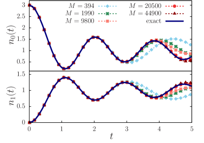
As shown in Fig. 8, this algebraic decay is well captured by NA-TEBD for short times, however, to capture the second oscillation, fairly large bond dimensions $\sim M\gtrsim 20,000$ are needed, corresponding to keeping $M_{\mathrm{mult}}=2500$ multiplets. With NA-TEBD simulations, we can easily reach these bond dimensions on a simple work station, which would be quite hopeless without exploiting the SU(3) symmetry.

We can test the accuracy of our computations also by investigating the increase of the bond entropy for $U=0$. We can compute this latter by using the approach of Peschel and Eisler.Peschel and Eisler (2009) To compute the entanglement entropy in a non-interacting system, we consider a long enough segment $L$ of the infinite one-dimensional system, and compute the correlator $C_{l,l^{\prime}\in\ L}(t)\equiv\left\langle\Psi(t)\right|c^{\dagger}_{l\alpha}c_{l^{\prime}\alpha}\left|\Psi(t)\right\rangle_{0}$, which, for a non-interacting system contains all information on the reduced density operator. The correlator $C_{l,l^{\prime}\in\ L}(t)$ can be evaluated along similar lines as the expectation value, $n_{0}(t)$, and is given by

$$C^{U=0}_{ll^{\prime}}(t)=\frac{1}{3}+\frac{1}{3}\,e^{i\frac{\pi}{3}(l+l^{\prime})}\big{(}1+e^{i\frac{\pi}{3}(l+l^{\prime})}\big{)}\,J_{l-l^{\prime}}(2Jt\sqrt{3})\;.$$ (23)

As shown in Ref. Peschel and Eisler, 2009, the entanglement entropy between the segment $L$ and the rest of the system can expressed just in terms of the eigenvalues $\xi$ of $C_{l,l^{\prime}\in\ L}(t)$ as

$$S^{L}_{\rm vN}(t)=-3\sum_{\xi}\big{(}\xi\ln(\xi)+(1-\xi)\ln(1-\xi)\big{)}\;,$$ (24)

where the factor 3 is due to the SU(3) flavor degeneracy. For large enough segments, this is just twice the entanglement entropy of two halves of an infinite system,

$$S_{\rm vN}(t)=\frac{1}{2}\lim_{L\to\infty}S^{L}_{\rm vN}(t)\;.$$ (25)

Computing the eigenvalues $\xi$ numerically, we can thus determine the complete time dependence of the entanglement entropy, $S_{\rm vN}(t)$.

Figure 9: Entropy growth for $U=0$, as a function of bond dimensions. Small oscillations are observed on top of an overall linear entropy growth. Very large ($M\approx 45,000$) effective bond dimensions are needed to recover the exact results (blue line) up to times $t\approx 4.5$.

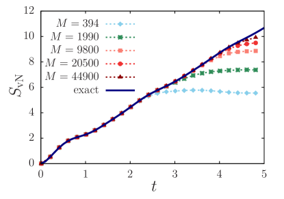
The (numerically determined) exact entanglement entropy is compared with the NA-TEBD results in Fig. 9. The initial state is a product state, and therefore completely unentangled at $t=0$. However, entanglement is generated with time. The Neumann entropy starts to increase roughly linearly, as predicted for gapless systems, Calabrese and Cardy (2005) but is modulated by small oscillations, reflecting the presence of coherent charge oscillations. NA-TEBD breaks down approximately where the bond dimension is insufficient to keep track of the entanglement entropy. In this gapless system, the conformal central charge is quite large, $c=3$, implying a fast increase of entanglement entropy. Indeed, numerical computations are quite demanding in this model, and bond dimensions in the range of $M\sim 40-50,000$ are needed to reach time scales $t\gtrsim 4J^{-1}$.

V.2 Interaction effects

Figure 10: Charge on the initially triple-occupied site as a function of time for different interaction strengths $U$. For small interaction strengths $U\lesssim 1.2$ we observe damped oscillations around the thermalized occupation $n=1$. Inset: extracted damping rate as a function of $U$.

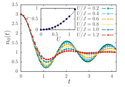
Interactions change the previous results dramatically. As shown in Fig. 10, charge oscillations become rapidly damped with increasing $U$. In the regime, $U\lesssim 1$, charge oscillations are suppressed exponentially in time compared to free fermion oscillations, $\delta n^{U\neq 0}_{0}(t)\propto e^{-\gamma\,t}\cdot J_{0}(2\sqrt{3}\,J\,t)$. The extracted damping rate $\gamma$ increases quadratically for small and moderate couplings, $U\lesssim 1$, as expected from perturbation theory, and shown in the inset of Fig. 10.

Figure 11: Connected part of charge-charge correlations computed for $U=1$. Correlations spread relativistically with a velocity $v\sim J$ for small and moderate values of $U$, but interactions quickly remove the oscillations and power-law correlations present in the non-interacting system.

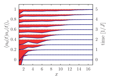
NA-TEBD can also be used to compute time dependent correlation functions. The precise numerical procedure is outlined in Appendices B and E. For the sake of simplicity, here we focus on the scalar operator, $\hat{n}_{l}$, which commutes with the symmetry generators, and is also completely local. For such operators, we can easily construct the ’reduced operator’, $\hat{O}_{l}\to O_{l}(\Gamma^{\mathrm{loc}}_{l})_{\tau}^{\tau^{\prime}}$ (see Appendix B), which acts directly on the the upper NA-MPS layer. From this point on, the computation of correlation functions follows the same line as for Abelian symmetries or non-symmetrical MPS states. Schollwöck (2011)

Fig. 11 shows the the time evolution of the connected correlator

$$C_{nn}^{\rm conn}(l,t)\equiv\langle\hat{n}_{0}(t)\hat{n}_{l}(t)\rangle-\langle\hat{n}_{0}(t)\rangle\langle\hat{n}_{l}(t)\rangle\,$$

for interaction strength $U=1$. The connected part of the correlation function is negative, indicating that excess particle densities emerge due to the quantum propagation of particles originally sitting at the origin. The connected negative correlations trace a light cone indicating that correlations and entanglement are both created by particles (or collectivemodes) traveling ballistically with a velocity $v\sim t$.

VI Numerical efficiency of NA-TEBD

Figure 12: CPU times of NA-MPS as a function of effective bond dimension, $M$, for calculations exploiting various symmetries. Using non-Abelian symmetries rather than Abelian ones speeds up the computations by almost two orders of magnitude.

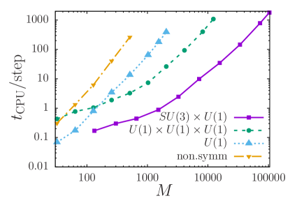
The SU(3) Hubbard model provides an ideal testbed to investigate the numerical efficiency of NA-TEBD. A detailed analysis of the run times and the memory usage is presented in Figs. 12 and 13, respectively.

Figs. 12 presents the CPU time as a function of effective bond dimension, $M$, for various symmetry combinations used. Using as many symmetries as possible makes our calculations tremendously efficient. Using just one U(1) symmetry speeds up the calculations by a factor of $\sim 20$, and we can gain an additional factor of $\sim 20$ in speed by exploiting the two additional U(1) symmetries. However, using SU(3)$\times$U(1) symmetry rather than U(1)$\times$U(1)$\times$U(1) increases the speed of our calculations by an additional factor of $\sim 100$, yielding an overall speed-up factor of about $\sim 100,000$.

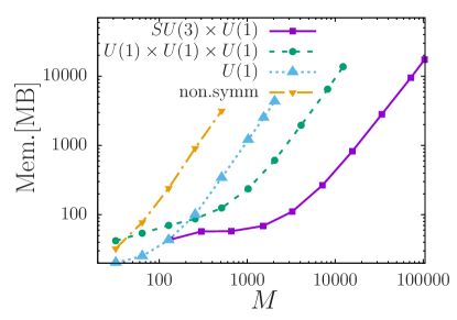
Similar efficiency is reached with memory storage space. With our 20 GB memory, we can reach bond dimensions of about $M\sim 1000$ without symmetries, $M\sim 10,000$ if we exploit the U(1)$\times$U(1)$\times$U(1) non-Abelian symmetry, but $M\sim 100,000$ if we use our non-Abelian approach. To reach these latter bond dimensions with just Abelian symmetries, one would need a memory of around $\sim 2\,\text{TB}$.

Figure 13: Memory usage of NA-MPS as a function of effective bond dimension $M$. Non-Abelian symmetries reduce memory usage with respect to Abelian computations by about two orders of magnitude, and allow to reach extremely high accuravy.

VII Conclusions

In this work, we gave a detailed description of our non-Abelian Matrix Product State (NA-MPS) approach, which we applied here for the SU(3) Hubbard model. We construct the MPS state as a two-layer structure, where the ’core’ of the MPS, i.e., the first layer is written in terms of multiplets, and tied through the so-called outer multiplicity labels to a second, Clebsch-Gordan layer. The latter can be consistently eliminated, thereby introducing a very efficient algorithm, where internal labels are suppressed. This approach leads to a 100-fold speed-up of the code and a 100-fold memory reduction with respect to simple Abelian codes in case of the SU(3) Hubbard model. We can thereby reach extremely large bond dimensions even on a small work station or even on a PC computer. This efficiency increase is even more dramatic for higher SU(N) symmetries, not studied here. This increased efficiency allows us to reach much better accuracies compared to codes using only Abelian symmetries. Unfortunately, the dramatic increase in bond dimensions amounts only in a relatively small (logarithmic) increase in the time span of our simulations in the particular case of the SU(3) Hubbard model.

We then introduced and NA-MPS based TEBD algorithm, NA-TEBD, which we used to investigate charge relaxation, starting from an initial state with three particles placed at every third site of the Hubbard chain. For $U=0$ we derived exact results for the single particle correlation functions, densities, and the entanglement entropy, which we used to benchmark our direct NA-TEBD simulations. In the absence of interactions, we observe algebraically decaying coherent charge oscillations, accompanied by a light-cone spread of correlations, and a linear growth of the entanglement entropy. Remarkably large bond dimensions were needed to capture even the first few oscillations in this non-interacting case.

Interactions induce exponential damping with a rate $\gamma\sim U^{2}$ for $U\lesssim 1$, indicative of a perturbative behavior for these moderate values of $U$. At the same time, the spread of correlations or the entropy growth rate remain barely affected.

The tensor structure developed is quite rich and opens many possibilities to study correlations and correlated dynamics: we can use it to construct tree tensor network states (NA-TTNS), or use them to study dissipative dynamics through Lindbladian evolution of matrix product operators (NA-MPO) with high accuracy using non-Abelian symmetries.Moca et al. Of course, we can also extend our approach to perform NA-DMRG calculations or NA-DM-NRG calculations.

Appendix A Description of non-trivial multiplets using NA-MPS

In the construction of NA-MPS (Section II.3) we used the fact that for a state $\left|\Psi\right\rangle$ belonging to the trivial representation $\Gamma=0$ the Schmidt-states can be sorted into multiplets. This statement is a consequence of the orthogonality theorem of group characters $\chi_{\Gamma}(g)=\mathrm{tr}\left\{R_{\Gamma}(g)\right\}$.Cornwell (1984) The orthogonality relation reads as $\int d\mu(g)\chi_{\Gamma_{1}}(g)\chi_{\Gamma_{2}}(g)^{*}=\delta_{\Gamma_{1},\Gamma_{2}}$. For direct products of representations the characters are simply multiplied, therefore the orthogonality relation introduces a constraint on the Clebsch-Gordan coefficients: the trivial representation ($\Gamma=0$) appears only in product spaces of representation – conjugate representation pairs, with outer multiplicity one. In all other products the trivial representation is missing. As a consequence of this constraint, for a trivial state $\left|\Psi\right\rangle$ the Schmidt pairs are members of multiplets that are conjugates of each other.

For a state $\left|\Psi_{\Gamma},m\right\rangle$ of a non-trivial representation $\Gamma\neq 0$, it is not possible to directly write the MPS in the form of (II.3), since Schmidt states obtained after decomposition are not sorted into multiplets. However, the problem can be circumvented by introducing an additional site that contains a multiplet for a single $\overline{{\Gamma}}$ representation. Using this auxiliary site we define a new pure state for the whole chain as

$$\left|\tilde{\Psi}\right\rangle=\sum_{m}\frac{1}{\sqrt{\dim(\Gamma)}}\left|\Psi_{\Gamma},m\right\rangle\left|\overline{\Gamma,m}\right\rangle\,,$$ (26)

where $\left|\overline{\Gamma,m}\right\rangle$ denotes the state at the auxiliary site. The $\left|\tilde{\Psi}\right\rangle$ state defined thus belongs to the trivial representation, i.e. it can be used to build an NA-MPS. The auxiliary site is placed in the rightmost position of the chain in our construction.

Performing a partial trace on $\left|\tilde{\Psi}\right\rangle$ over the auxiliary site state, we obtain the density matrix of the real system.

$$\hat{\rho}=\sum_{m}\frac{1}{\dim(\Gamma)}\left|\Psi_{\Gamma},m\right\rangle\left\langle\Psi_{\Gamma},m\right|\;.$$ (27)

Appendix B NA-MPS states

In this section we present some details on how the reduced matrix elements, like the reduced evolver in Fig. 7 can be constructed by employing the Clebsch-Gordan coefficients’ sum rule. We start with a short description on how to perform the scalar product of two NA-MPSs.

Figure 14: (a) Scalar product of two NA-MPS’s. The symbol ’*’ attached to a tensor indicates the complex conjugation. (b) As a result of Eq. (28), the Clebsch-Gordan tensors (formally introduced) at the first grid location are dropped. (c-d) Visualising the contraction of the Clebsch layer by using the orthogonality equation (29) and constructing the so called ’reduced scalar product’.

B.1 Scalar product

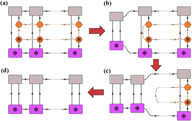
In Fig. 14 (a) we introduce the graphical representation for the scalar product of two NA-MPS’s, which, by ’integrating’ the Clebsches layer, can be simplified to what we call ’reduced scalar product’, i.e. a scalar product involving only the upper MPS layer (displayed in Fig. 14.d).

First, we formally add a trivial site to the left belonging to the representation $\Gamma_{0}=0$. The appearing $C(\Gamma_{0}=0,\Gamma^{\mathrm{loc}}_{1},\Gamma_{1})_{0\,\mu_{1}}^{m_{1}\,\alpha}$ Clebsch-Gordan coefficients imply that $\alpha$ is one-dimensional, since $0\otimes\Gamma^{\mathrm{loc}}_{1}$ contains only one multiplet of $\Gamma^{\mathrm{loc}}_{1}$, and furthermore

$$C(\Gamma_{0}=0,\Gamma^{\mathrm{loc}}_{1},\Gamma_{1})_{0\,\mu_{1}}^{m_{1}\,\alpha=1}=\delta_{\Gamma^{\mathrm{loc}}_{1}}^{\Gamma_{1}}\delta_{\mu_{1}}^{m_{1}}\;.$$ (28)

Using this equation, we graphically obtain the result presented in Fig. 14.b. To move on, we use the orthogonality relation

$$\sum_{m,\mu}C(\Gamma,\Gamma^{\mathrm{loc}},\Gamma^{\prime})_{m\,\mu^{\prime}}^{m^{\prime}\,\alpha}\left(C(\Gamma,\Gamma^{\mathrm{loc}},\tilde{\Gamma}^{\prime})_{m\,\mu^{\prime}}^{\tilde{m}^{\prime}\,\tilde{\alpha}}\right)^{*}=\delta_{\tilde{\Gamma}^{\prime}}^{\Gamma^{\prime}}\delta_{\tilde{m}^{\prime}}^{m^{\prime}}\delta_{\tilde{\alpha}}^{\alpha},\;$$ (29)

to eliminate locally the Clebsch-Gordan tensors and move site by site (a typical iteration is presented in Fig. 14.c), to finally reach the right end of the chain (displayed in Fig. 14.d), where the layers of $C$ tensors have disappeared from the expression, that is, the scalar product of the full NA-MPSs is given by the ’reduced scalar product’ of the upper layers.

Notice the double line structure connecting the two NA-MPS states: the first line carries the label of a local multiplet, while the second line carries the outer mupltiplicity labels, $\alpha$, assuring via their dependencies that representation labels of corresponding bonds and local states all match in both states.

B.2 Matrix elements of scalar operators

Figure 15: Left: Matrix element of a scalar operator $\hat{O}$ between two Schmidt states. Right: Definition of the reduced matrix element of the scalar operator as in Eq. (31).

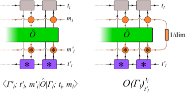
Let us consider an operator $\hat{O}$, which only acts on a spatially localized subset of sites on the left of bond $l$. For now, we assume that this operator is a ’scalar’, i.e., it commutes with all symmetry operations $\hat{U}(g)$. A trivial example in case of the SU(3) Hubbard model is the particle number operator, $n_{l}=\sum_{\alpha}c^{\dagger}_{l\alpha}c_{l\alpha}$, or any function of this operator. Another (not independent) example is the Casimir operator ${{\cal C}_{l}}=\sum_{i}\hat{\lambda}_{l}^{i}\hat{\lambda}_{l}^{i}$. These operators belong to the trivial representation $\Gamma=0$. Therefore acting with them on a Schmidt state does not change the quantum numbers of the latter. In general, we can therefore write (see also Fig. 15).

$$\phantom{)}_{l}\left\langle\Gamma^{\prime};t^{\prime},m^{\prime}\right|\hat{O}\left|\Gamma;t,m\right\rangle_{l}=\delta_{\Gamma^{\prime}}^{\Gamma}\delta_{m^{\prime}}^{m}O(\Gamma)_{t^{\prime}}^{t}\;.$$ (30)

The reduced matrix elements $O(\Gamma_{l})_{t^{\prime}}^{t}$ can be easily obtained by tracing over $m$ and $m^{\prime}$,

$$O(\Gamma)_{t^{\prime}}^{t}=\frac{1}{\dim(\Gamma)}\sum_{m}\,{}_{l}\left\langle\Gamma;t^{\prime},m\right|\hat{O}\left|\Gamma;t,m\right\rangle_{l}\;.$$ (31)

This relationship is shown in the right panel of Fig. 15. The rectangular box labeled as ’1/dim’ , represents the operation $\frac{1}{\dim(\Gamma)}\delta_{m}^{m^{\prime}}$ that again can be represented as an NA-tensor. Eq. (30) is a special case of the Wigner-Eckart theorem for scalar operators. The general case is discussed in Appendix E.

Appendix C The upper layer of the NA-MPS

As we have discussed in Sec. II.3, in the NA-TEBD algorithm, the upper layer of the NA-MPS can be treated in all respects as a conventional MPS state (without symmetry). We now show in detail that the upper layer of the NA-MPS does indeed encode an MPS state, but on a very complicated basis of Hilbert space.

Consider the NA-MPS state defined in Eq. (II.3) and represented in Fig. 5. The lower layer specifies the following product states (complemented with the auxiliary site introduced in Appendix A),

$$\left|\left\{\Gamma\right\}^{[1]},\tau_{1},\alpha_{1};\;\left\{\Gamma\right\}^{[2]},\tau_{2},\alpha_{2};\;\dots;\;\left\{\Gamma\right\}^{[L]},\tau_{L},\alpha_{L}\right\rangle = \sum_{\left\{\mu_{l}\right\}}\sum_{\left\{m_{l}\right\}}C(\left\{\Gamma\right\}^{[1]})_{0\;\mu_{1}}^{m_{1}\;\alpha_{1}}\,C(\left\{\Gamma\right\}^{[2]})_{m_{1}\,\mu_{2}}^{m_{2}\;\alpha_{2}}\dots C(\left\{\Gamma\right\}^{[L]})_{m_{L-1}\,\mu_{L}}^{0\;\alpha_{L}}$$ (32)

$$\times \left|\Gamma^{\mathrm{loc}}_{1}\;\tau_{1},\mu_{1}\right\rangle\otimes\left|\Gamma^{\mathrm{loc}}_{2}\;\tau_{2},\mu_{2}\right\rangle\otimes\dots\otimes\left|\Gamma^{\mathrm{loc}}_{L}\;\tau_{L},\mu_{L}\right\rangle\ .$$

Here, as before, $\left\{\Gamma\right\}^{[l]}=(\Gamma_{l-1},\Gamma^{\mathrm{loc}}_{l},\Gamma_{l})$ and $\Gamma_{0}=\Gamma_{L}=0$. These states span the singlet sector of the Hilbert space of the chain (extended by the auxiliary site at the right most position), and form an orthonormal basis due to the orthogonality relation of the Clebsch-Gordan coefficients, Eq. (29). The state notation is slightly redundant, since representation sets $\left\{\Gamma\right\}^{[l]}$ and $\left\{\Gamma\right\}^{[l+1]}$ at adjacent grid positions share the same $\Gamma_{l}$ representation index. This constraint will be essential in determining the Schmidt decomposition of the state. We can write an arbitrary singlet state on this basis as

$$\left|\Psi\right\rangle=\sum_{\left\{\Gamma^{\mathrm{loc}}_{l}\right\}}\sum_{\left\{\Gamma_{l}\right\}}\sum_{\left\{\tau_{l}\right\}}\sum_{\left\{\alpha_{l}\right\}} \Psi_{\left\{\Gamma\right\}^{[1]},\tau_{1},\alpha_{1};\;\left\{\Gamma\right\}^{[2]},\tau_{2},\alpha_{2};\;\dots;\;\left\{\Gamma\right\}^{[L]},\tau_{L},\alpha_{L}}\left|\left\{\Gamma\right\}^{[1]},\tau_{1},\alpha_{1};\;\left\{\Gamma\right\}^{[2]},\tau_{2},\alpha_{2};\;\dots;\;\left\{\Gamma\right\}^{[L]},\tau_{L},\alpha_{L}\right\rangle\;.$$

To build the MPS, we need a Schmidt decomposition of this state, that translates to the SVD of the $\Psi_{\dots}$ expansion coefficient. First we need to divide the indices into two parts. Let the cut position be between the sites $l$ and $l+1$. Then by performing the SVD of the coefficient, we get the following expression,

$$\Psi_{\left\{\left\{\Gamma\right\}^{[1]},\tau_{1},\alpha_{1};\;\dots\;;\left\{\Gamma\right\}^{[l]},\tau_{l},\alpha_{l}\right\}\;\left\{\left\{\Gamma\right\}^{[l+1]},\tau_{l+1},\alpha_{l};\;\dots\;;\left\{\Gamma\right\}^{[L]},\tau_{L},\alpha_{L}\right\}}=\\ \phantom{asssssssssssss}\sum_{t_{l}}U_{\left\{\left\{\Gamma\right\}^{[1]},\tau_{1},\alpha_{1};\;\dots\;;\left\{\Gamma\right\}^{[l]},\tau_{l},\alpha_{l}\right\}\;t_{l}}\;\Lambda^{[l]}(\Gamma_{l})_{t_{l}}\;V_{t_{l}\;\left\{\left\{\Gamma\right\}^{[l+1]},\tau_{l+1},\alpha_{l+1};\;\dots\;;\left\{\Gamma\right\}^{[L]},\tau_{L},\alpha_{L}\right\}}\;.$$ (33)

The $\left\{\Gamma\right\}^{[l]}$ and $\left\{\Gamma\right\}^{[l+1]}$ representation sets contain the common representation $\Gamma_{l}$, so by performing SVD, the Schmidt values $\Lambda^{[l]}(\Gamma_{l})_{t_{l}}$ are also labeled according to $\Gamma_{l}$. Eq. (33) is analogous to the nonsymmetric equation, therefore the rows of the $U$ matrix and the columns of the $V$ matrix are again orthonormal (half-unitarity), and the normalization condition $\left\langle\Psi|\Psi\right\rangle=1$ translates to

$$\sum_{\Gamma_{l}}\sum_{t_{l}}\left|\Lambda^{[l]}(\Gamma_{l})_{t_{l}}\right|^{2}=1.$$ (34)

The previously introduced left-canonical $A^{[l]}$ tensor is defined by $U$, while the right-canonical states can be defined in a similar way using the $V$ matrices

$$U_{\left\{\left\{\Gamma\right\}^{[1]},\tau_{1},\alpha_{1};\;\dots\;;\left\{\Gamma\right\}^{[l]},\tau_{l},\alpha_{l}\right\}\;t_{l}}=\sum_{t_{l-1}}\sum_{\tau_{l}}\sum_{\alpha_{l}}U_{\left\{\left\{\Gamma\right\}^{[1]},\tau_{1},\alpha_{1};\;\dots\;;\left\{\Gamma\right\}^{[l-1]},\tau_{l-1},\alpha_{l-1}\right\}\;t_{l-1}}A^{[l]}(\left\{\Gamma\right\}^{[l]})_{t_{l-1}\,\tau_{l}\,\alpha_{l}}^{t_{l}}\\ V_{t_{l}\;\left\{\left\{\Gamma\right\}^{[l+1]},\tau_{l+1},\alpha_{l};\;\dots\;;\left\{\Gamma\right\}^{[L]},\tau_{L},\alpha_{L}\right\}}=\sum_{t_{l+1}}\sum_{\tau_{l+1}}\sum_{\alpha_{l+1}}B^{[l+1]}(\left\{\Gamma\right\}^{[l+1]})_{\tau_{l+1}\,\alpha_{l+1}\,t_{l+1}}^{t_{l}}V_{t_{l+1}\;\left\{\left\{\Gamma\right\}^{[l+1]},\tau_{l+2},\alpha_{l+2};\;\dots\;;\left\{\Gamma\right\}^{[L]},\tau_{L},\alpha_{L}\right\}}\;.$$ (35)

From the half-unitarity of U and V-matrices, we imitedly get the half-unitarity of the $A^{[l]}$ and $B^{[l]}$ tensors, as well as the relation between them.

$$\sum_{\Gamma_{l-1}}\sum_{\Gamma^{\mathrm{loc}}_{l}}\sum_{t_{l-1}}\sum_{\tau_{l}}\sum_{\alpha_{l}}A^{[l]}(\left\{\Gamma\right\}^{[l]})_{t_{l-1}\,\tau_{l}\,\alpha_{l}}^{t_{l}}\left(A^{[l]}(\left\{\Gamma\right\}^{[l]})_{t_{l-1}\,\tau_{l}\,\alpha_{l}}^{t_{l}^{\prime}}\right)^{*} = \delta_{t_{l}^{\prime}}^{t_{l}}\;$$ (36)

$$\sum_{\Gamma_{l+1}}\sum_{\Gamma^{\mathrm{loc}}_{l}}\sum_{t_{l+1}}\sum_{\tau_{l+1}}\sum_{\alpha_{l+1}}B^{[l+1]}(\left\{\Gamma\right\}^{[l+1]})_{\tau_{l+1}\,\alpha_{l+1}\,t_{l+1}}^{t_{l}}\left(B^{[l+1]}(\left\{\Gamma\right\}^{[l+1]})_{\tau_{l+1}\,\alpha_{l+1}\,t_{l+1}}^{t_{l}^{\prime}}\right)^{*} = \delta_{t_{l}^{\prime}}^{t_{l}}\;$$ (37)

$$A^{[l]}(\left\{\Gamma\right\}^{[l]})_{t_{l-1}\,\tau_{l}\,\alpha_{l}}^{t_{l}}\;\Lambda^{[l]}(\Gamma_{l})t_{l}=\Lambda^{[l-1]}(\Gamma_{l-1})\;B^{[l]}(\left\{\Gamma\right\}^{[l]})_{\tau_{l}\,\alpha_{l}\,t_{l}}^{t_{l-1}}$$ (38)

These equations are completely analogous to the orthogonality equations Eq. (5) for the first, left-canonical matrix.

To conclude this appendix, we can say that the upper layer of the NA-MPS state can be understood as a conventional MPS wave function interpreted on a basis defined in Eq. (32). The resulting Schmidt weights and the properties of the left and right canonical tensors are similar to those of the regular MPSs, so adapting already developed algorithms to our NA-MPS and eliminating the Clebsch-Gordan layer does not require conceptual modifications.

Appendix D Details of the implementation of NA-TEBD

In Sec. IV.2 we briefly introduced the basic steps to implement the NA-TEBD algorithm. In this Appendix, we present the technical details of the implementation. Let’s first consider the equation defining the reduced evolver $U_{\mathrm{red}}$ graphically defined in Fig. 7,

$$U_{\mathrm{red}}\left(\Gamma_{l-1},\Gamma^{\mathrm{loc}}_{l},\Gamma_{l},{\Gamma^{\mathrm{loc}}_{l}}^{\prime},\Gamma_{l}^{\prime},\Gamma^{\mathrm{loc}}_{l+1},{\Gamma^{\mathrm{loc}}_{l+1}}^{\prime},\Gamma_{l+1}\right)_{\tau_{l}^{\prime}\,\alpha_{l}^{\prime}\;\tau_{l+1}^{\prime},\alpha_{l+1}^{\prime}}^{\tau_{l}\,\alpha_{l}\;\tau_{l+1}\,\alpha_{l+1}}=\sum_{m_{l-1}}\sum_{\mu_{l}}\sum_{m_{l}}\sum_{\mu_{l+1}}\sum_{m_{l+1}}\sum_{\mu_{l}^{\prime}}\sum_{m_{l}^{\prime}}\sum_{\mu_{l+1}^{\prime}}\frac{1}{\dim(\Gamma_{l+1})}\times\\ C(\Gamma_{l-1},\Gamma^{\mathrm{loc}}_{l},\Gamma_{l})_{m_{l-1}\,\mu_{l}}^{m_{l}\,\alpha_{l}}\;C(\Gamma_{l},\Gamma^{\mathrm{loc}}_{l+1},\Gamma_{l+1})_{m_{l}\,\mu_{l+1}}^{m_{l+1}\,\alpha_{l+1}}\;U(\Gamma^{\mathrm{loc}}_{l},\Gamma^{\mathrm{loc}}_{l+1},{\Gamma^{\mathrm{loc}}_{l}}^{\prime},{\Gamma^{\mathrm{loc}}_{l+1}}^{\prime})_{\tau_{l}^{\prime}\,\mu_{l}^{\prime}\;\tau_{l+1}^{\prime},\mu_{l+1}^{\prime}}^{\tau_{l}\,\mu_{l}\;\tau_{l+1}\,\mu_{l+1}}\times\\ \left(C(\Gamma_{l-1},{\Gamma^{\mathrm{loc}}_{l}}^{\prime},\Gamma_{l}^{\prime})_{m_{l-1}\,\mu_{l}^{\prime}}^{m_{l}^{\prime}\,\alpha_{l}^{\prime}}\right)^{*}\left(C(\Gamma_{l}^{\prime},{\Gamma^{\mathrm{loc}}_{l+1}}^{\prime},\Gamma_{l+1})_{m_{l}^{\prime}\,\mu_{l+1}^{\prime}}^{m_{l+1}\,\alpha_{l+1}^{\prime}}\right)^{*}\;.$$ (39)

We now explicitly display representation indices that label the blocks of each tensor. As stated in Sec. IV.2, the blocks of the reduced tensor $U_{\mathrm{red}}$ have a total of eight representation indices.

We want to formulate TEBD for purely left-canonical MPS’s, but this requires some tricks Vidal (2007a), since SVD always results in a left-canonical and a right-canonical tensor. The algorithm can be constructed in four steps:

1. Contract the tensors $A^{[l]}$ and $A^{[l+1]}$ for the two neighboring sites,

   $$W(\Gamma_{l-1},\Gamma^{\mathrm{loc}}_{l},\Gamma_{l},\Gamma^{\mathrm{loc}}_{l+1},\Gamma_{l+1})_{t_{l-1}\,\tau_{l}\,\alpha_{l}\,\tau_{l+1}\,\alpha_{l+1}}^{t_{l+1}}=\sum_{t_{l}}A^{[l]}(\Gamma_{l-1},\Gamma^{\mathrm{loc}}_{l},\Gamma_{l})_{t_{l-1}\,\tau_{l}\,\alpha_{l}}^{t_{l}}A^{[l+1]}(\Gamma_{l},\Gamma^{\mathrm{loc}}_{l+1},\Gamma_{l+1})_{t_{l}\,\tau_{l+1}\,\alpha_{l+1}}^{t_{l+1}}\;.$$ (40)

2. Construct the time evolved tensor,

   $$\widetilde{W}(\Gamma_{l-1},{\Gamma^{\mathrm{loc}}_{l}}^{\prime},{\Gamma_{l}}^{\prime},{\Gamma^{\mathrm{loc}}_{l+1}}^{\prime},\Gamma_{l+1})_{t_{l-1}\,\tau_{l}^{\prime}\,\alpha_{l}^{\prime}\,\tau_{l+1}^{\prime}\,\alpha_{l+1}^{\prime}}^{t_{l+1}}=\sum_{\Gamma^{\mathrm{loc}}_{l}}\sum_{\Gamma^{\mathrm{loc}}_{l+1}}\sum_{\Gamma_{l}}\sum_{\tau_{l}}\sum_{\alpha_{l}}\sum_{\tau_{l+1}}\sum_{\alpha_{l+1}}\times\\ U_{\mathrm{red}}\left(\Gamma_{l-1},\Gamma^{\mathrm{loc}}_{l},\Gamma_{l},{\Gamma^{\mathrm{loc}}_{l}}^{\prime},\Gamma_{l}^{\prime},\Gamma^{\mathrm{loc}}_{l+1},{\Gamma^{\mathrm{loc}}_{l+1}}^{\prime},\Gamma_{l+1}\right)_{\tau_{l}^{\prime}\,\alpha_{l}^{\prime}\;\tau_{l+1}^{\prime},\alpha_{l+1}^{\prime}}^{\tau_{l}\,\alpha_{l}\;\tau_{l+1}\,\alpha_{l+1}}W(\Gamma_{l-1},\Gamma^{\mathrm{loc}}_{l},\Gamma_{l},\Gamma^{\mathrm{loc}}_{l+1},\Gamma_{l+1})_{t_{l-1}\,\tau_{l}\,\alpha_{l}\,\tau_{l+1}\,\alpha_{l+1}}^{t_{l+1}}\;.$$ (41)

3. On the right, we multiply by the appropriate Schmidt weights,

   $$\tilde{\Theta}(\Gamma_{l-1},{\Gamma^{\mathrm{loc}}_{l}}^{\prime},{\Gamma_{l}}^{\prime},{\Gamma^{\mathrm{loc}}_{l+1}}^{\prime},\Gamma_{l+1})_{t_{l-1}\,\tau_{l}^{\prime}\,\alpha_{l}^{\prime}\,\tau_{l+1}^{\prime}\,\alpha_{l+1}^{\prime}}^{t_{l+1}}=\widetilde{W}(\Gamma_{l-1},{\Gamma^{\mathrm{loc}}_{l}}^{\prime},{\Gamma_{l}}^{\prime},{\Gamma^{\mathrm{loc}}_{l+1}}^{\prime},\Gamma_{l+1})_{t_{l-1}\,\tau_{l}^{\prime}\,\alpha_{l}^{\prime}\,\tau_{l+1}^{\prime}\,\alpha_{l+1}^{\prime}}^{t_{l+1}}\Lambda^{[l+1]}(\Gamma_{l+1})_{t_{l+1}}\,.$$ (42)

   This step is essential for numerical stability.

4. Execute the SVD on the $\tilde{\Theta}$ tensor. We can do this separately for each block in ${\Gamma_{l}}^{\prime}$,

   $$\tilde{\Theta}(\Gamma_{l-1},{\Gamma^{\mathrm{loc}}_{l}}^{\prime},{\Gamma_{l}}^{\prime},{\Gamma^{\mathrm{loc}}_{l+1}}^{\prime},\Gamma_{l+1})_{t_{l-1}\,\tau_{l}^{\prime}\,\alpha_{l}^{\prime}\,\tau_{l+1}^{\prime}\,\alpha_{l+1}^{\prime}}^{t_{l+1}}\Rightarrow\sum_{t_{l}^{\prime}}\tilde{A}^{[l]}(\Gamma_{l-1},{\Gamma^{\mathrm{loc}}_{l}}^{\prime},{\Gamma_{l}}^{\prime})_{t_{l-1}\,\tau_{l}^{\prime}\,\alpha_{l}^{\prime}}^{t_{l}^{\prime}}\times\\ \phantom{abcdefghijkl}\tilde{\Lambda}^{[l]}({\Gamma_{l}}^{\prime})_{t_{l}^{\prime}}\tilde{B}^{[l+1]}({\Gamma_{l}}^{\prime},{\Gamma^{\mathrm{loc}}_{l+1}}^{\prime},\Gamma_{l+1})_{t_{l}^{\prime}\,\tau_{l+1}^{\prime}\,\alpha_{l+1}^{\prime}}^{t_{l+1}}\;.$$ (43)

5. The new $\tilde{A}^{[l+1]}$ tensor for the right site is obtained from $\widetilde{W}$ by utilizing the orthogonality equation, Eq. (36),

   $$\tilde{A}^{[l+1]}({\Gamma_{l}}^{\prime},{\Gamma^{\mathrm{loc}}_{l+1}}^{\prime},\Gamma_{l+1})_{t_{l}^{\prime}\,\tau_{l+1}^{\prime}\,\alpha_{l+1}^{\prime}}^{t_{l+1}}=\sum_{\Gamma_{l-1}}\sum_{{\Gamma^{\mathrm{loc}}_{l}}^{\prime}}\sum_{t_{l-1}}\sum_{\tau_{l}^{\prime}}\sum_{\alpha_{l}^{\prime}}\widetilde{W}(\Gamma_{l-1},{\Gamma^{\mathrm{loc}}_{l}}^{\prime},{\Gamma_{l}}^{\prime},{\Gamma^{\mathrm{loc}}_{l+1}}^{\prime},\Gamma_{l+1})_{t_{l-1}\,\tau_{l}^{\prime}\,\alpha_{l}^{\prime}\,\tau_{l+1}^{\prime}\,\alpha_{l+1}^{\prime}}^{t_{l+1}}\times\\ \left(\tilde{A}^{[l]}(\Gamma_{l-1},{\Gamma^{\mathrm{loc}}_{l}}^{\prime},{\Gamma_{l}}^{\prime})_{t_{l-1}\,\tau_{l}^{\prime}\,\alpha_{l}^{\prime}}^{t_{l}^{\prime}}\right)^{*}$$ (44)

Apparently, the algorithm can be implemented using purely left-canonical $A^{[l]}$ tensors, but we also need to store and update the $\Lambda^{[l]}(\Gamma_{l})_{t_{l}}$ Schmidt weights, provided by the SVD step 4.

Appendix E Handling non-scalar operators

In the NA-TEBD algorithm, we have seen that the reduced shape of a scalar operator belonging to two adjacent lattice sites can be easily determined by contractions with Clebsch-Gordan tensors. However, this method is difficult to generalize for handling distant interactions, or for calculating distant correlations, since the reduced coupling contains all the lattice locations between interacting lattices at once, meaning that we would store a huge multi-lattice operator, which quickly leads to depletion of computing and storage capacities. This problem can be circumvented by generalizing Eq. (30), which is possible by the Wigner-Eckart theorem. For this we need the notion of irreducible tensor operators (henceforth simply tensor operators). These are operator multiples of $\hat{O}({\Gamma_{\mathrm{op}}})^{M}$, with ($M\in\{1\dots\dim{\Gamma_{\mathrm{op}}})\}$), which are transformed by $\hat{\mathcal{U}}(g)$ symmetry transforms as represented by $\Gamma_{\mathrm{op}}$, as follows,

$$\hat{\mathcal{U}}(g)\;\hat{O}({\Gamma^{\mathrm{op}}})^{M}\;\hat{\mathcal{U}}(g)^{\dagger}=\sum_{M^{\prime}}\left[R_{\Gamma^{\mathrm{op}}}\right]_{M^{\prime}}^{M}\hat{O}(\Gamma^{\mathrm{op}})^{M^{\prime}}\;.$$ (45)

As an example, consider the standard spin operator, which is the combination of the three spin components ($\hat{S}^{x}$, $\hat{S}^{y}$, $\hat{S}^{z}$). The spin operators form a three-dimensional ($S_{\mathrm{op}}=1$) multiplet, whose elements

$$\hat{S}^{M}=\left(-\hat{S}^{+}/{\sqrt{2}}\,,\;\hat{S}^{z}\,,\;\hat{S}^{-}/{\sqrt{2}}\right)\;,$$ (46)

provided that the state space is expressed in the basis of the eigenvalues of the spin component $\hat{S}^{z}$. Here $\hat{S}^{\pm}=\hat{S}^{x}\pm i\hat{S}^{y}$ are the usual spin-shift operators.

The Wigner-Eckart theorem follows from the observation that if we act on the states of a multiplet of a representation $\Gamma$ with elements of the operator multiplet of $\Gamma_{\mathrm{op}}$, the result will transform under the product representation $\Gamma\otimes\Gamma_{\mathrm{op}}$. This product can be grouped again into multiplets using the Clebsch-Gordan coefficients. Therefore, for the matrix elements of the tensor operators we obtain the following equation,

$$\left\langle\Gamma^{\prime};t^{\prime},m^{\prime}\right|\hat{O}(\Gamma^{\mathrm{op}})^{M}\left|\Gamma;t,m\right\rangle=\sum_{\alpha}\mathbb{O}(\left\{\Gamma\right\})_{t^{\prime}}^{t\;\alpha}\left(C(\left\{\Gamma\right\})_{m\,M}^{m^{\prime}\,\alpha}\right)^{*}\;,$$ (47)

where $\left\{\Gamma\right\}=(\Gamma,\Gamma^{\mathrm{op}},\Gamma^{\prime})$ represents the representation indices that appear. Comparing this with Eq. (30) we notice that $\mathbb{O}{\left\{\Gamma\right\}}_{t^{\prime}}^{t\;\alpha}$ is a reduced matrix element, but it contains three different representation indices for general tensor operators and an $\alpha$ outer-multiplicity index that is contracted with the Clebsch-Gordan tensor.

The reduced matrix element can be obtained from Eq. (47) using the orthogonality relation Eq. (29)

$$\mathbb{O}(\left\{\Gamma\right\})_{t^{\prime}}^{t\;\alpha}=\sum_{m,m^{\prime},M}\frac{1}{\dim(\Gamma^{\prime})}\;C(\left\{\Gamma\right\})_{m\,M}^{m^{\prime}\,\alpha}\;\left\langle\Gamma^{\prime};t^{\prime},m^{\prime}\right|\hat{O}(\Gamma_{\mathrm{op}})^{M}\left|\Gamma;t,m\right\rangle\;.$$ (48)

References

- Krishna-murthy et al. (1980a) H. R. Krishna-murthy, J. W. Wilkins, and K. G. Wilson, Phys. Rev. B 21, 1003 (1980a).
- Krishna-murthy et al. (1980b) H. R. Krishna-murthy, J. W. Wilkins, and K. G. Wilson, Phys. Rev. B 21, 1044 (1980b).
- White (1992) S. R. White, Phys. Rev. Lett. 69, 2863 (1992).
- Schollwöck (2005) U. Schollwöck, Rev. Mod. Phys. 77, 259 (2005).
- Schollwöck (2011) U. Schollwöck, Annals of Physics 326, 96 (2011).
- Vidal (2004) G. Vidal, Phys. Rev. Lett. 93, 040502 (2004).
- Vidal (2007a) G. Vidal, Phys. Rev. Lett. 98, 070201 (2007a).
- White and Feiguin (2004) S. R. White and A. E. Feiguin, Phys. Rev. Lett. 93, 076401 (2004).
- Haegeman et al. (2011) J. Haegeman, J. I. Cirac, T. J. Osborne, I. Pižorn, H. Verschelde, and F. Verstraete, Phys. Rev. Lett. 107, 070601 (2011).
- Verstraete et al. (2008) F. Verstraete, V. Murg, and J. Cirac, Advances in Physics 57, 143 (2008).
- Orús (2014) R. Orús, Annals of Physics 349, 117 (2014).
- Vidal (2007b) G. Vidal, Phys. Rev. Lett. 99, 220405 (2007b).
- Gunst et al. (2018) K. Gunst, F. Verstraete, S. Wouters, Ö. Legeza, and D. Van Neck, Journal of Chemical Theory and Computation 14, 2026 (2018) .
- Nakatani and Chan (2013) N. Nakatani and G. K.-L. Chan, The Journal of Chemical Physics 138, 134113 (2013).
- Szalay et al. (2015) S. Szalay, M. Pfeffer, V. Murg, G. Barcza, F. Verstraete, R. Schneider, and Ö. Legeza, International Journal of Quantum Chemistry 115, 1342 (2015).
- Lubasch et al. (2014) M. Lubasch, J. I. Cirac, and M.-C. Bañuls, Phys. Rev. B 90, 064425 (2014).
- Corboz (2016) P. Corboz, Phys. Rev. B 94, 035133 (2016).
- (18) ITENSOR software package .
- Bauer et al. (2011) B. Bauer, L. D. Carr, H. G. Evertz, A. Feiguin, J. Freire, S. Fuchs, L. Gamper, J. Gukelberger, E. Gull, S. Guertler, A. Hehn, R. Igarashi, S. V. Isakov, D. Koop, P. N. Ma, P. Mates, H. Matsuo, O. Parcollet, G. Pawłowski, J. D. Picon, L. Pollet, E. Santos, V. W. Scarola, U. Schollwöck, C. Silva, B. Surer, S. Todo, S. Trebst, M. Troyer, M. L. Wall, P. Werner, and S. Wessel, Journal of Statistical Mechanics: Theory and Experiment 2011, P05001 (2011).
- Tóth et al. (2008) A. I. Tóth, C. P. Moca, Ö. Legeza, and G. Zaránd, Phys. Rev. B 78, 245109 (2008).
- Moca et al. (2012) C. P. Moca, A. Alex, J. von Delft, and G. Zaránd, Phys. Rev. B 86, 195128 (2012).
- McCulloch and Gulácsi (2002) I. P. McCulloch and M. Gulácsi, Europhysics Letters (EPL) 57, 852 (2002).
- Singh et al. (2010) S. Singh, H.-Q. Zhou, and G. Vidal, New Journal of Physics 12, 033029 (2010).
- Gunst et al. (2019) K. Gunst, F. Verstraete, and D. Van Neck, Journal of chemical theory and computation 15, 2996 (2019).
- Hubig (2018) C. Hubig, SciPost Physics 5, 047 (2018).
- Werner et al. (2019) M. A. Werner, C. P. Moca, Ö. Legeza, M. Kormos, and G. Zaránd, Phys. Rev. B 100, 035401 (2019).
- Weichselbaum (2012) A. Weichselbaum, Annals of Physics 327, 2972 (2012).
- Weichselbaum (2020) A. Weichselbaum, Phys. Rev. Research 2, 023385 (2020).
- Wigner (1959) E. P. Wigner, Group Theory and its Application to the Quantum Mechanics of Atomic Spectra (Academic Press, 1959).
- Hofstetter et al. (2002) W. Hofstetter, J. I. Cirac, P. Zoller, E. Demler, and M. D. Lukin, Phys. Rev. Lett. 89, 220407 (2002).
- Boll et al. (2016) M. Boll, T. A. Hilker, G. Salomon, A. Omran, J. Nespolo, L. Pollet, I. Bloch, and C. Gross, Science 353, 1257 (2016).
- Trotzky et al. (2012) S. Trotzky, Y.-A. Chen, A. Flesch, I. P. McCulloch, U. Schollwöck, J. Eisert, and I. Bloch, Nature Physics 8, 325 (2012).
- Schmidt (2907) E. Schmidt, Math. Ann. 63, 433 (2907).
- Cornwell (1984) J. F. Cornwell, Group Theory in Physics, Volume II (Academic Press London, 1984).
- Roy and Banerjee (2014) A. Roy and S. Banerjee, Linear algebra and matrix analysis for statistics (Chapman and Hall/CRC, 2014).
- Note (1) In case of multiple symmetries like each label is alone a combination of two quantum numbers, specifying an SU(3) representation (Young tableau) and a U(1) charge. Then a block of an NA-tensor is addressed by a set of such combined representation labels.
- Žnidarič et al. (2008) M. Žnidarič, T. Prosen, and P. Prelovšek, Phys. Rev. B 77, 064426 (2008).
- Bardarson et al. (2012) J. H. Bardarson, F. Pollmann, and J. E. Moore, Phys. Rev. Lett. 109, 017202 (2012).
- Pozsgay et al. (2014) B. Pozsgay, M. Mestyán, M. A. Werner, M. Kormos, G. Zaránd, and G. Takács, Phys. Rev. Lett. 113, 117203 (2014).
- Schreiber et al. (2015) M. Schreiber, S. S. Hodgman, P. Bordia, H. P. Luschen, M. H. Fischer, R. Vosk, E. Altman, U. Schneider, and I. Bloch, Science 349, 842 (2015).
- Else et al. (2016) D. V. Else, B. Bauer, and C. Nayak, Phys. Rev. Lett. 117, 090402 (2016).
- Trotter (1959) H. F. Trotter, Proceedings of the American Mathematical Society 10, 545 (1959).
- Suzuki (1976) M. Suzuki, Communications in Mathematical Physics 51, 183 (1976).
- Note (2) This is different from SU(2), where every Young tableau consists of a single line of length , with the usual spin.
- Peschel and Eisler (2009) I. Peschel and V. Eisler, Journal of Physics A: Mathematical and Theoretical 42, 504003 (2009).
- Calabrese and Cardy (2005) P. Calabrese and J. Cardy, Journal of Statistical Mechanics: Theory and Experiment 2005, P04010 (2005).
- (47) C. P. Moca, M. A. Werner, Ö. Legeza, and G. Zaránd, work in progress .