Coulomb electron pairing in a tight-binding model of La-based cuprate superconductors

Abstract

We study the properties of two electrons with Coulomb interactions in a tight-binding model of La-based cuprate superconductors. This tight-binding model is characterized by long-range hopping obtained previously by advanced quantum chemistry computations. We show analytically and numerically that the Coulomb repulsion leads to a formation of compact pairs propagating through the whole system. The mechanism of pair formation is related to the emergence of an effective narrow energy band for Coulomb electron pairs with conserved total pair energy and momentum. The dependence of the pair formation probability on an effective filling factor is obtained with a maximum around a filling factor of 20 (or 80) percent. The comparison with the case of the nearest neighbor tight-binding model shows that the long-range hopping provides an increase of the phase space volume with high pair formation probability. We conjecture that the Coulomb electron pairs discussed here may play a role in high temperature superconductivity.

1 Introduction

The phenomenon of high temperature superconductivity (HTC), discovered in [1], still requires its detailed physical understanding as discussed by various experts of this field (see e.g. [2, 3, 4]). The analysis is complicated by the complexity of the phase diagram and strong interactions between electrons (or holes). As a generic model, that can be used for a description of most superconducting cuprates, it was proposed to use a simplified one-body Hamiltonian with nearest-neighbor hopping on a square lattice formed by the Cu ions [5]. In addition the interactions between electrons are considered as a strongly screened Coulomb interaction that results in the 2D Hubbard model [5]. However, a variety of experimental results cannot be described by the 2D Hubbard model (see e.g. discussion in [6]). Other models of type Emery [7, 8, 9, 10] were developed and extended on the basis of extensive computations with various numerical methods of quantum chemistry (see e.g. [11, 6] and Refs. therein). These studies demonstrated the importance of next-nearest hopping and allowed to determine reliably the longer-ranged tight-binding parameters.

In this work we use the 2D longer-ranged tight-binding parameters reported in [6] and study the effects of Coulomb interactions between electrons in the frame work of this tight-binding model. There are different reasons indicating that long-range interactions between electrons may lead to certain new features as compared to the Hubbard case (see [3, 4, 6]). Recently, we demonstrated that for two electrons on a 2D lattice with nearest-neighbor hopping the energy and momentum conservation laws leads to appearance of an effective narrow energy band for energy dispersion of two electrons [12]. In such a narrow band even a repulsive Coulomb interaction leads to electron pairing and ballistic propagation of such pairs through the whole system. The internal classical dynamics of electrons inside such a pair is chaotic suggesting nontrivial properties of pair formation in the quantum case. In this work we extend the investigations of the properties of such Coulomb electron pairs for a more generic longer-ranged tight-binding lattice of one-body Hamiltonian typical for La-based cuprate superconductors. We find that the long-range hopping leads to new features of Coulomb electron pairs.

In Sec. 2 a detailed description of the tight-binding model for two interacting electrons for general lattices with a particular application to HTC is presented together with an analysis of the effective band width at fixed conserved total pair momentum. Section 3 provides first results of the full space time evolution obtained in the frame work of the Trotter formula approximation. Section 4 introduces the theoretical basis for the description in terms of an effective block Hamiltonian for a given sector of fixed momentum of a pair with technical details provided in Appendix A. In Sec. 5 the phase diagram of the long time average of the pair formation probability in the plane of total momentum is discussed while Sec. 6 provides some results for the intermediate time evolution of pair formation. An overview of the results for the pair formation probability at different filling factors is given in Section 7. The final discussion is presented in Section 8.

2 Generalized tight-binding model on a 2D lattice

We assume that each electron moves on a square lattice of size $N\times N$ with periodic boundary conditions with respect to the following generalized one-particle tight-binding Hamiltonian:

$$H_{1p}=-\sum_{{\bf r}}\sum_{{\bf a}\in{\cal A}}t_{\bf a}\,\bigl{(}|{\bf r}\rangle\langle{\bf r}+{\bf a}|+|{\bf r}+{\bf a}\rangle\langle{\bf r}|\bigr{)}$$ (1)

where the first sum is over all discrete lattice points ${\bf r}$ (measured in units of the lattice constant) and ${\bf a}$ belongs to a certain set of neighbor vectors ${\cal A}$ such that for each lattice state $|{\bf r}\rangle$ there are non-vanishing hopping matrix elements $t_{\bf a}$ with $|{\bf r}+{\bf a}\rangle$ and $|{\bf r}-{\bf a}\rangle$ for ${\bf a}\in{\cal A}$. To be more precise, due to notational reasons, we choose the set ${\cal A}$ to contain all neighbor vectors ${\bf a}=(a_{x},a_{y})$ in one half plane with either $a_{x}>0$ or $a_{y}>0$ if $a_{x}=0$ such that ${\cal A}^{\prime}={\cal A}\cup(-{\cal A})$ is the full set of all neighbor vectors. For each vector ${\bf a}$ of the full set ${\cal A}^{\prime}$, we require that any other vector $\tilde{\bf a}$ which can be obtained from ${\bf a}$ by a reflection at either the $x$-axis, $y$-axis or the $x$-$y$ diagonal also belongs to the full set ${\cal A}^{\prime}$ and has the same hopping amplitude $t_{\bf a}=t_{\tilde{\bf a}}$.

For the usual nearest neighbor tight-binding model (NN-model), already considered in [12], we have the set ${\cal A}_{\rm NN}=\{(1,0),(0,1)\}$ with $t_{(1,0)}=t_{(0,1)}=t=1$. The numerical results presented in this work correspond either to the NN-model (for illustration and comparison) or to a longer-ranged tight-binding lattice according to [6] which we denote as the HTC-model. For this case the set of neighbor vectors is ${\cal A}_{\rm HTC}=\{(1,0),(0,1),(2,0),(0,2),$ $(1,\pm 2),(2,\pm 1),(1,\pm 1),(2,\pm 2)\}$ and the hopping amplitudes are: $t=t_{(1,0)}=1$, $t^{\prime}=t_{(1,1)}=-0.136$, $t{{}^{\prime\prime}}=t_{(2,0)}=0.068$, $t{{}^{\prime\prime\prime}}=t_{(2,1})=0.061$ and $t^{(4)}=t_{(2,2)}=-0.017$ corresponding to the values given in Table 2 of [6] (all energies are measured in units of the hopping amplitude $t=t_{(1,0)}=t_{(0,1)}$ which is therefore set to unity here; see also Fig. 6a of [6] for the neighbor vectors of the different hopping amplitudes). The hopping amplitudes for other vectors such as $(0,1)$, $(1,-1)$, $(2,1)$, $(1,-2)$ etc. are obtained from the above amplitudes by the appropriate symmetry transformations, e.g. $t_{(1,-1)}=t_{(1,1)}=t^{\prime}=-0.136$ etc.

Even though that most of our numerical results presented in this work apply to the HTC-model (or the NN-model), we emphasize that certain theoretical considerations given below, especially for the effective block Hamiltonian in relative coordinates at given total momentum, are valid for arbitrary generalized tight binding models with more general sets ${\cal A}$ and also with a potential generalization to other dimensions.

The eigenstates of $H_{1p}$ given in (1) are simple plane waves:

$$|{\bf p}\rangle=\frac{1}{N}\sum_{\bf r}\,e^{i{\bf p}\cdot{\bf r}}$$ (2)

with energy eigenvalues:

$$E_{1p}({\bf p})=-2\sum_{{\bf a}\in{\cal A}}t_{\bf a}\cos({\bf p}\cdot{\bf a})$$ (3)

and momenta ${\bf p}=(p_{x},p_{y})$ such that $p_{x}$ and $p_{y}$ are integer multiples of $2\pi/N$ (i.e. $p_{\alpha}=2\pi l_{\alpha}/N$, $l_{\alpha}=0,\ldots,N-1$, $\alpha=x,y$). For the HTC model, we can give a more explicit expression of the energy dispersion:

$$E_{1p} (p_{x},p_{y})=-2\left[\cos(p_{x})+\cos(p_{y})\right]$$ (4)

$$-4t^{\prime}\cos(p_{x})\cos(p_{y})-2t{{}^{\prime\prime}}\left[\cos(2p_{x})+\cos(2p_{y})\right]$$

$$-4t{{}^{\prime\prime\prime}}\left[\cos(2p_{x})\cos(p_{y})+\cos(2p_{y})\cos(p_{x})\right]$$

$$-4t^{(4)}\cos(2p_{x})\cos(2p_{y})$$

which corresponds to eq. (30) of [6] (assuming $t=1$ and $t^{(5)}=t^{(6)}=t^{(7)}=0$).

The quantum Hamiltonian of the model with two interacting particles (TIP) has the form:

$$H=H_{1p}^{(1)}\otimes{\bf 1}^{(2)}+{\bf 1}^{(1)}\otimes H_{1p}^{(2)}+\sum_{{\bf r}_{1},{\bf r}_{2}}\bar{U}({\bf r}_{2}-{\bf r}_{1})|{\bf r}_{1},{\bf r}_{2}\rangle\langle{\bf r}_{1},{\bf r}_{2}|$$ (5)

where $H_{1p}^{(j)}$ is the one-particle Hamiltonian (1) of particle $j=1,2$ with positional coordinate ${\bf r}_{j}=(x_{j},y_{j})$ and ${\bf 1}^{(j)}$ is the unit operator of particle $j$. The last term in (5) represents a (regularized) Coulomb type long-range interaction $\bar{U}({\bf r}_{2}-{\bf r}_{1})=U/[1+r({\bf r}_{2}-{\bf r}_{1})]$ with amplitude $U$ and the effective distance $r({\bf r}_{2}-{\bf r}_{1})=\sqrt{\Delta\bar{x}^{2}+\Delta\bar{y}^{2}}$ between the two electrons on the lattice with periodic boundary conditions. (Here $\Delta\bar{x}=\min(\Delta x,N-\Delta x)$; $\Delta\bar{y}=\min(\Delta y,N-\Delta y)$; $\Delta x=x_{2}-x_{1}$; $\Delta y=y_{2}-y_{1}$ and the latter differences are taken modulo $N$, i.e. $\Delta x=N+x_{2}-x_{1}$ if $x_{2}-x_{1}<0$ and similarly for $\Delta y$). Furthermore, we consider symmetric (spatial) wavefunctions with respect to particle exchange assuming an antisymmetric spin-singlet state (similar results are obtained for antisymmetric wavefunctions).

In absence of interaction ($U=0$) the energy eigenvalues (the classical energy) of the two electron Hamiltonian (5) (the two electrons) at given momenta ${\bf p}_{1}$ and ${\bf p}_{2}$ are (is) given by:

$$E_{c}({\bf p}_{1},{\bf p}_{2}) =E_{1p}({\bf p}_{1})+E_{1p}({\bf p}_{2})$$ (6)

$$=-4\sum_{{\bf a}\in{\cal A}}t_{\bf a}\cos({\bf p}_{+}\cdot{\bf a}/2)\cos(\Delta{\bf p}\cdot{\bf a})$$

where ${\bf p}_{+}={\bf p}_{1}+{\bf p}_{2}$ is the total momentum and $\Delta{\bf p}=({\bf p}_{2}-{\bf p}_{1})/2$ is the momentum associated to the relative coordinate $\Delta{\bf r}={\bf r}_{2}-{\bf r}_{1}$. For the NN-model Eq. (6) becomes $E_{c}({\bf p}_{1},{\bf p}_{2})=-4\sum_{\alpha=x,y}\cos(p_{+\alpha}/2)\cos(\Delta p_{\alpha})$.

Due to the translational invariance the total momentum ${\bf p}_{+}$ is conserved even in the presence of interaction ($U\neq 0$) and only two-particle plane wave states with identical ${\bf p}_{+}$ are coupled by non-vanishing interaction matrix elements. For the case of the NN-model, analyzed in [12], the kinetic energy at fixed ${\bf p}_{+}$ is bounded by $\Delta E_{b}=4\sum_{\alpha=x,y}|\cos(p_{+\alpha}/2)|$. Thus for TIP states with $E>\Delta E_{b}$ the two electrons cannot separate and propagate as one pair even if their interaction is repulsive. For $p_{+x}=p_{+y}=\pi+\delta$ being close to $\pi$ and $|\delta|\ll 1$ there are compact Coulomb electron pairs even for very small interactions $U$ as soon as $\Delta E_{b}\approx 4|\delta|<U\ll B_{2}$ with $B_{2}=16+U$ being the maximal energy bandwidth in 2D. Thus the conservation of the total momentum of a pair with $p_{+x}=p_{+y}\approx\pi$ leads to the appearance of an effective narrow energy band with formation of coupled electron pairs propagating through the whole system. However, the results obtained in [12] show that even for other values of $p_{+x},p_{+y}$ the probability of pair formation is rather high.

For the NN-model the effective band width for pairs $\Delta E_{b}$ can be exactly zero for the specific pair momentum ${\bf p}_{+}=(\pi,\pi)$. However, this is not the case for the HTC-model where due to the longer-ranged hopping the minimal width $\Delta E_{b}$ is finite due to the additional terms with factors $\cos({\bf p}_{+}\cdot{\bf a}/2)$ in (6). Therefore, we determined numerically for each given value of total momentum ${\bf p}_{+}$ the effective bandwidth as:

$$\Delta E_{b}({\bf p}_{+})=\max_{\Delta{\bf p}}\left[E_{c}({\bf p}_{1},{\bf p}_{2})\right]-\min_{\Delta{\bf p}}\left[E_{c}({\bf p}_{1},{\bf p}_{2})\right]$$ (7)

with ${\bf p}_{1}={\bf p}_{+}/2-\Delta{\bf p}$ and ${\bf p}_{2}={\bf p}_{+}/2+\Delta{\bf p}$. Top panels of Fig. 1 show density color plots of $\Delta E_{b}({\bf p}_{+})$ for the NN- and the HTC-model. For the HTC-case $\Delta E_{b}({\bf p}_{+})$ is maximal at ${\bf p}_{+}=(0,0)$ with value $\Delta E_{b,\rm max}=17.952$ and minimal at ${\bf p}_{+}=(\pi,\pi)$ with value $\Delta E_{b,\rm min}=2.176$ while for the NN-model we have $\Delta E_{b,\rm max}=16$ at ${\bf p}_{+}=(0,0)$ and $\Delta E_{b,\rm min}=0$ at ${\bf p}_{+}=(\pi,\pi)$. The value $\Delta E_{b,\rm min}=2.176$ for the HTC-model is still rather small compared to the maximal value $\Delta E_{b,\rm max}\approx 18$ and we may expect a somewhat stronger pair formation probability for total momenta ${\bf p}_{+}$ close to $(\pi,\pi)$. However, this situation is qualitatively different as compared to the NN-model and the HTC-case requires new careful studies.

For comparison, we also show in the lower panels of Fig. 1 the kinetic energy $E_{c}$ at ${\bf p}_{1}={\bf p}_{2}={\bf p}_{+}/2$ (for the square ${\bf p}_{+}\in[0,\pi]\times[0,\pi]$) corresponding to $\Delta{\bf p}=0$. While for the NN-model this quantity vanishes at ${\bf p}_{+}=(\pi,\pi)$ there is for the HTC-model a zero-line between the two points $(\beta\pi,\pi)$ and $(\pi,\beta\pi)$ where $\beta\approx 0.877\approx 7/8$ is a numerical constant slightly below unity.

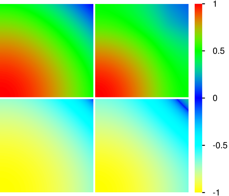
Figure 1: Top panels show the dependence of the effective electron pair band width $\Delta E_{b}({\bf p}_{+})$ on the pair momentum ${\bf p}_{+}=(p_{+x},p_{+y})$. Bottom panels show the kinetic electron pair energy $E_{c}({\bf p}_{1},{\bf p}_{2})$ (in absence of interaction) at momenta ${\bf p}_{1}={\bf p}_{2}={\bf p}_{+}/2$. Left panels correspond to the NN-model and right panels to the HTC-model. In all panels the horizontal axis corresponds to $p_{+x}\in[0,\pi]$ and the vertical axis to $p_{+y}\in[0,\pi]$. The numbers of the color bar correspond for top panels to the ratio of the bandwidth over its maximal value and for lower panels to the quantity $\operatorname{sgn}(E_{c})\sqrt{|E_{c}|/E_{c,{\rm max}}}$ with $E_{c,{\rm max}}$ being the maximum of $|E_{c}|$. In all subsequent color plot figures the numerical values of the color bar corresponds to the ratio of the shown quantity over its maximal value.

3 Full space time evolution of electron pairs

As in [12] the full time evolution of two electrons is computed numerically for $N=128$ using the Trotter formula approximation (see e.g. [12, 13] for computational details). We use the Trotter time step $\Delta t=B_{2}=1/(16+U)$ which is the inverse bandwidth for the case of NN-model. A further decrease of the time step does not affect the obtained results. At the initial time both electrons are localized approximately at $(N/2,N/2)$ with the distance $\Delta\bar{x}=\Delta\bar{y}=1$ using a linear combination of 8 states with all combinations due to particle exchange symmetry and reflection symmetry at the $\Delta x$- and $\Delta y$-axis. The method provides for each time value a wavefunction $\psi(x_{1},y_{1},x_{2},y_{2})$ from which we extract different quantities such as the density in $x_{1}$-$x_{2}$ plane:

$$\rho_{XX}(x_{1},x_{2})=\sum_{y_{1},y_{2}}|\psi(x_{1},y_{1},x_{2},y_{2})|^{2}$$ (8)

or the density $\Delta x$-$\Delta y$ plane:

$$\rho_{\rm rel}(\Delta x,\Delta y)=\sum_{x_{1},x_{2}}|\psi(x_{1},y_{1},x_{1}+\Delta x,y_{1}+\Delta y)|^{2}$$ (9)

(with position sums taken modulo $N$). We also compute the quantity $w_{10}$ by summing the latter density (9) over all values such that $|\Delta\bar{x}|\leq 10$ and $|\Delta\bar{y}|\leq 10$ which corresponds to a square of size $21\times 21$ in $\Delta x$-$\Delta y$ plane (due to negative values of $x_{2}-x_{1}$ etc.). This quantity gives the quantum probability to find both electrons at a distance $\leq 10$ (in each direction) and we will refer to it as the pair formation probability.

In Fig. 2 the density $\rho_{XX}$ is shown for $U=2$, both NN- and HTC-models at two time values $t=445\Delta t$ and $t=10^{4}\,\Delta t$. These results show that the wavefunction has a component with electrons separating from each other and a component where electrons stay close to each other forming a pair propagating through the whole system that corresponds to a high density near a diagonal with $x_{1}\approx x_{2}$. For $t=445\Delta t$ the value of $w_{10}$ is roughly 10% and for $t=10^{4}\,\Delta t$ it is roughly 13% for both models. However, the remaining diffusing component of about 87-90% probability has a stronger periodic structure for the NN-model as compared to the HTC-model.

Figure 3 shows the density $\rho_{\rm rel}(\Delta x,\Delta y)$ for the same cases of Fig. 2. We clearly see a strong enhancement of the probability at small values $\Delta\bar{x}\approx\Delta\bar{y}<5$ ($<6-7$) for the NN-model (HTC-model) showing that there is a considerable probability that both electrons stay close to each other forming a Coulomb electron pair. Furthermore, the remaining wavefunction component of independently propagating electrons, clearly visible in Fig. 2, is not visible in the density shown in Fig. 3 even though this component corresponds to 87-90% probability.

The supplementary material contains two videos (for $\sim 460$ time values in the range $\Delta t\leq t\leq 10^{4}\Delta t$ with roughly uniform logarithmic density) of the two densities $\rho_{XX}$ and $\rho_{\rm rel}$ where both models NN and HTC are directly compared in the same video. The raw-data used for these videos is the same as in Figs. 2 and 3.

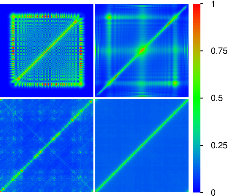
Figure 2: 2D Wavefunction density $\rho_{XX}(x_{1},x_{2})$ in $x_{1}$-$x_{2}$ plane (see Eq. (8)) obtained from the time evolution using the Trotter formula approximation for initial electron positions at $\approx(N/2,N/2)$ with distance $\Delta\bar{x}=\Delta\bar{y}=1$ for $N=128$, $U=2$ and Trotter integration time step $\Delta t=1/B_{2}=1/(16+U)$. Top (bottom) panels correspond to the time value $t=445\,\Delta t$ ($t=10^{4}\Delta t$) and left (right) panels correspond to the NN-lattice (HTC-lattice). The corresponding values of the pair formation probability $w_{10}$ are 0.106 (top left), 0.133 (bottom left), 0.0940 (top right) and 0.125 (bottom right). Related videos are available at [14, 15].

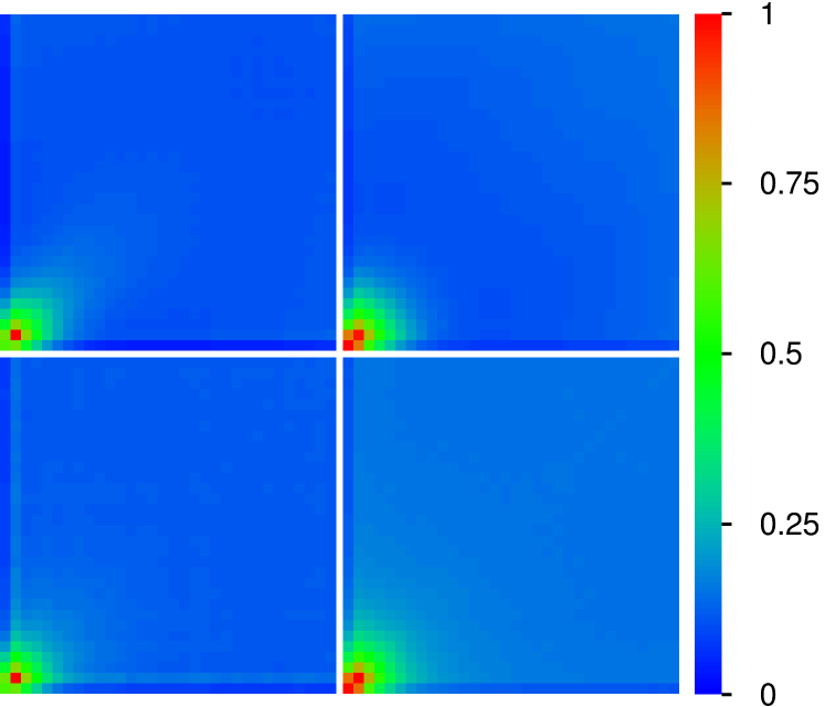
Figure 3: 2D Wavefunction density $\rho_{\rm rel}(\Delta x,\Delta y)$ in $\Delta x$-$\Delta y$ plane of relative coordinates (see Eq. (9)) for the same states, cases and parameters of Fig. 2. All panels show the zoomed density for $0\leq\Delta x,\Delta y<32$. Related videos are available at [14, 15].

4 Time evolution in sectors of fixed total momentum

As already mentioned in Sec. 3 the total momentum ${\bf p}_{+}$ is conserved by the TIP dynamics of the Hamiltonian (5). In order to exploit this more explicitly, we introduce as in [12], block basis states by:

$$|{\bf p}_{+},{\Delta{\bf r}}\rangle=\frac{1}{N}\sum_{{\bf r}_{1}}e^{i{\bf p}_{+}\cdot({\bf r}_{1}+{\Delta{\bf r}}/2)}|{\bf r}_{1},{\bf r}_{1}+{\Delta{\bf r}}\rangle$$ (10)

where ${\bf p}_{+}=(p_{+x},p_{+y})$ (with $p_{+\alpha}=2\pi l_{+\alpha}/N$; $l_{+\alpha}=0,\ldots,N-1$; $\alpha=x,y$) is a fixed value of the total momentum and ${\bf r}_{1}$, ${\Delta{\bf r}}$ are vectors on the square lattice (with position sums in each spatial direction taken modulo $N$). One can show (see Appendix A for details) that the TIP Hamiltonian (5) applied to such state gives a linear combination of such states for different ${\Delta{\bf r}}$ values but the same total momentum value ${\bf p}_{+}$ which provides for each value or sector of ${\bf p}_{+}$ an effective block Hamiltonian:

$$\bar{h}^{({\bf p}_{+})}= -\sum_{{\Delta{\bf r}}}\sum_{{\bf a}\in{\cal A}}\bar{t}^{({\bf p}_{+})}_{\bf a}\bigl{(}|{\Delta{\bf r}}+{\bf a}\rangle\langle{\Delta{\bf r}}|+|{\Delta{\bf r}}\rangle\langle{\Delta{\bf r}}+{\bf a}|\bigr{)}$$ (11)

$$+\sum_{{\Delta{\bf r}}}\bar{U}({\Delta{\bf r}})|{\Delta{\bf r}}\rangle\langle{\Delta{\bf r}}|$$

where $\bar{t}^{({\bf p}_{+})}_{\bf a}=2\cos({\bf p}_{+}\cdot{\bf a}/2)\,t_{\bf a}$ is an effective rescaled hopping amplitude depending also on ${\bf p}_{+}$ and we have for simplicity omitted the index ${\bf p}_{+}$ in the block basis states. This effective block Hamiltonian corresponds to a tight-binding model in 2D of similar structure as (1) with modified hopping amplitudes and an additional “potential” $\bar{U}({\Delta{\bf r}})$. We note that in absence of this external potential ($U=0$) the eigenfunctions of (11) are plane waves and we immediately recover the expression (6) for its energy eigenvalues where $\Delta{\bf p}$ is the momentum associated to the relative coordinate ${\Delta{\bf r}}$. For the simple NN-model the result for the effective block Hamiltonian was already given in [12] and the above expression (11) provides the generalization to arbitrary tight-binding lattices characterized by a certain set of neighbor vectors ${\cal A}$ and associated hopping amplitudes $t_{\bf a}$ (the generalization to arbitrary spatial dimension is also obvious). As already discussed in [12] the boundary conditions of (11) in $x-$ ($y-$)direction are either periodic if the integer index $l_{+x}$ ($l_{+y}$) of $p_{+x}$ ($p_{+y}$) is even or anti-periodic if this index is odd. This can be understood by the fact that the expression (10) is modified by the factor $e^{\pm ip_{+x}N/2}=e^{\pm i\pi l_{+x}}=(-1)^{l_{+x}}$ if $\Delta x$ is replaced by $\Delta x\pm N$ and similarly for $\Delta y$ (with ${\Delta{\bf r}}=(\Delta x,\Delta y))$.

Diagonalizing the effective block Hamiltonian (11), we can rather efficiently compute the exact quantum time evolution $|\bar{\psi}(t)\rangle=e^{-i\bar{h}^{({\bf p}+)}\,t}\,|\bar{\psi}(0)\rangle$ inside a given sector of ${\bf p}_{+}$. As initial state $|\bar{\psi}(0)\rangle$ we choose a state (in the reduced block space) given as the totally symmetric superposition of four localized states where $\Delta x$ and $\Delta y$ are either 1 or $N-1$. Such a state corresponds in full space to a plane wave in the center of mass direction with total fixed momentum ${\bf p}_{+}$ and strongly localized in the relative coordinate ${\Delta{\bf r}}$. The matrix size of (11) is $N^{2}$ which corresponds to a complexity of $N^{6}$ for the numerical diagonalization.

However, for a general lattice, such as the HTC-model, one can exploit the particle exchange symmetry to reduce the effective matrix size to roughly $N^{2}/2$ and for the special cases of $p_{+x}=p_{+y}$ or either $p_{+x}=0$ or $p_{+y}=0$ a second symmetry allows a further reduction of the effective matrix size to $\approx N^{2}/4$ (for the NN-model there are two or three symmetries for these cases with effective matrix sizes of $\approx N^{2}/4$ or $\approx N^{2}/8$ respectively; see [12] and Appendix A for details).

In view of this, we have been able to compute numerically the exact time evolution for the HTC-model in certain ${\bf p}_{+}$ sectors for a lattice size up to $N=384$ for the case of two symmetries and a limited number of different other parameters (values of ${\bf p}_{+}$ and $U$). For the case of one symmetry and the exploration of all possible values of $p_{+x}$ and $p_{+y}$ we used the maximum system size $N=192$. We also implemented more expensive computations where no or less possible symmetries are used to verify (at smaller values of $N$) that they provide identical numerical results.

We compute the wavefunction in block representation $\bar{\psi}({\bf p}_{+},{\Delta{\bf r}})$ for about 700 time values $t=0$ and $10^{-1}\leq t/\Delta t\leq 10^{6}$ (with a uniform density in logarithmic scale) where $\Delta t=1/B_{2}=1/(16+U)$ is the time step already used for the Trotter formula approximation given as the inverse bandwidth for the case of the NN-model which is the smallest time (inverse of the largest energy) scale of the system.

From the wavefunction we extract in a similar way as in Sec. 3 the pair formation probability $w_{10}$ by summing the (normalized) wavefunction density $|\bar{\psi}({\bf p}_{+},{\Delta{\bf r}})|^{2}$ at fixed ${\bf p}_{+}$ over the $21\times 21$ square with $|\Delta\bar{x}|\leq 10$ and $|\Delta\bar{y}|\leq 10$. We also compute the inverse participation ratio:

$$\xi_{\rm IPR}=\left(\sum_{\Delta{\bf r}}|\bar{\psi}({\bf p}_{+},{\Delta{\bf r}})|^{4}\right)^{-1}$$ (12)

which gives roughly the number of lattice sites (in ${\Delta{\bf r}}$ space) over which the wavefunction is localized. Both quantities $w_{10}$ and $\xi_{\rm IPR}$ converge typically rather well to their stationary values at times $t>10^{3}\Delta t$ with some time dependent fluctuations. Therefore for the cases where we are interested in the long time limit we compute the wavefunction only for 70 times values (in the same interval as above with uniform logarithmic density) and take the average over the 21 values with $10^{4}\leq t/\Delta t\leq 10^{6}$. We note that for the case of a uniform wavefunction density the ergodic values are $w_{10,\rm erg}=(21/N)^{2}$ and $\xi_{\rm IPR,erg}=N^{2}$. Values of $w_{10}$ significantly above $w_{10,\rm erg}$ or of $\xi_{\rm IPR}$ below $\xi_{\rm IPR,erg}$ indicate an enhanced probability for the formation of compact electron pairs.

We also mention that both quantities $w_{10}$ and $\xi_{\rm IPR}$ are invariant with respect to the three transformations $p_{+x}\leftrightarrow p_{+y}$, $p_{+x}\to-p_{+x}$ and $p_{+y}\to-p_{+y}$ (or $p_{+x}\to 2\pi-p_{+x}$ and $p_{+y}\to 2\pi-p_{+y}$) corresponding to reflections at the $x$-$y$ diagonal, the $y$-axis and the $x$-axis. Even though the effective block Hamiltonian (11) is not (always) invariant with respect to all three of these transformations (see Appendix A for details), the choice of an invariant initial state ensures that at finite times the wavefunction in block space satisfies for example the identity $\bar{\psi}(p_{+x},p_{+y},\Delta x,\Delta y)=\bar{\psi}(p_{+y},p_{+x},\Delta y,\Delta x)$ (and similarly for the other reflections). In other words a certain reflection transformation for ${\bf p}_{+}$ results in the equivalent transformation for the time dependent block space wavefunction in ${\Delta{\bf r}}$ space. Obviously the two quantities $w_{10}$ and $\xi_{\rm IPR}$ do not change with respect to these transformations (in ${\Delta{\bf r}}$ space) and therefore they are conserved. As a result it is sufficient to compute these quantities only for the triangle $0\leq p_{+y}\leq p_{+x}\leq\pi$.

In the following sections we present the results for these quantities and the wavefunction in block representation.

5 Phase diagram of pair formation

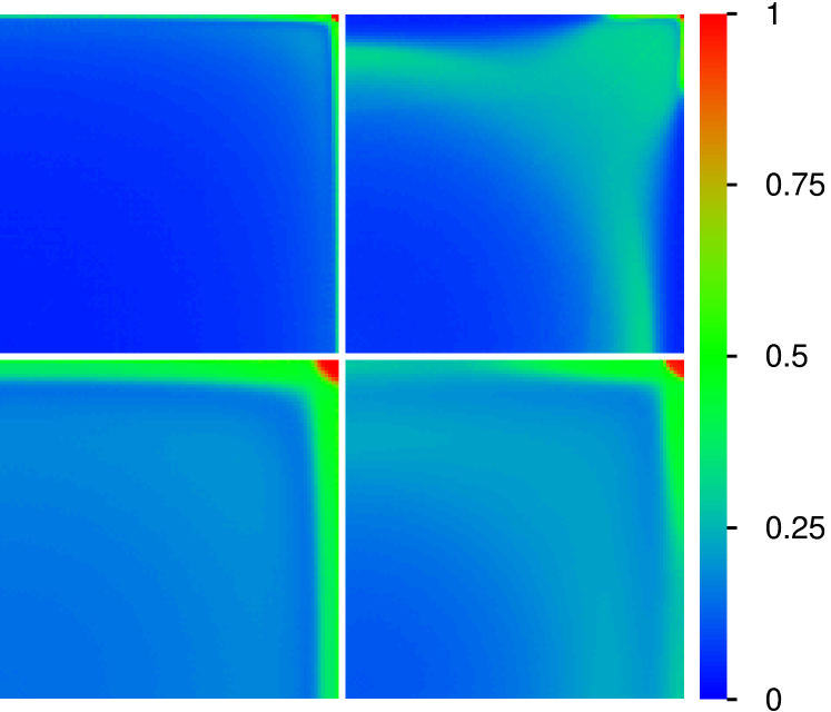
Figure 4: Phase diagram of electron pair formation in the plane of pair momentum ${\bf p}_{+}=(p_{+x},p_{+y})$ for the NN-lattice (left panels), the HTC-lattice (right panels) and the interaction values $U=0.5$ (top panels), $U=2$ (bottom panels). Shown is the pair formation probability $w_{10}$ for $N=192$ obtained from the exact time evolution for each sector of ${\bf p}_{+}$ with an initial electron distance $\Delta\bar{x}=\Delta\bar{y}=1$ and computed from an average over 21 time values in the interval $10^{4}\leq t/\Delta t\leq 10^{6}$. In all panels the horizontal (vertical) axis corresponds to $p_{+x}\;(p_{+y})\;\in[0,\pi]$ and the numerical values of the color bar correspond to the ratio of $w_{10}$ over its maximal value. The maximum values corresponding to the red region at the top right corner ${\bf p}_{+}=(\pi,\pi)$ are $w_{10}=1$ (both left panels), $w_{10}=0.4510$ (top right) and $w_{10}=0.8542$ (bottom right). For comparison the ergodic value is $w_{10,\rm erg.}=(21/192)^{2}=0.01196$.

The phase diagram of the long time average of the pair formation probability $w_{10}$ in the ${\bf p}_{+}$-plane is shown in Fig. 4 for both models and the interaction values $U=0.5,\,2$. As expected from the features of the effective bandwidth shown in (the top panels of) Fig. 1, we find that globally for both models the pair formation probability is clearly maximal at ${\bf p}_{+}=(\pi,\pi)$ and minimal at ${\bf p}_{+}=(0,0)$. Furthermore, the size of the maximum region is significantly stronger for $U=2$ than for $U=0.5$ which is also to be expected. Thus for these ${\bf p}_{+}$ values even a relatively weak or moderate Coulomb repulsion creates quite strongly coupled electron pairs.

For the NN-model the top ($p_{+y}=\pi$) or right ($p_{+x}=\pi$) boundary also provide large values with $w_{10}\approx 0.5$ and the width of these regions is stronger for $U=2$ than for $U=0.5$. However, for $U=2$ also the remaining region provides values between 0.14 and 0.25 of the maximum value which are clearly above the ergodic value 0.012. Even for $U=0.5$ the remaining region is mostly $\approx 0.04$ (with some part close to 0.25) which is still above the ergodic value.

For the HTC-model the situation is more complicated. The boundary regions are more limited, especially for $U=0.5$. However, for the remaining region there is a new interesting feature which is a significantly enhanced “green-circle” of approximate radius $r_{g}=\sqrt{{p^{2}}_{+x}+{p^{2}}_{+y}}\approx 0.85\pi$ for $U=0.5$ ($w_{10}\approx 0.14$). For $U=2$ there is also a circle ($w_{10}\approx 0.20$) with approximate radius $r_{g}\approx 0.75\pi$. This circle seems to be less pronounced despite its larger value of $w_{10}$ as compared to $U=0.5$ due to the fact that the maximum value for $U=2$ ($w_{10}\approx 0.85$ at ${\bf p}_{+}=(\pi,\pi)$) is roughly twice the maximum value for $U=0.5$ ($w_{10}\approx 0.45$). This structure cannot be explained by the behavior of the effective bandwidth. The minimum values of $w_{10}$ at ${\bf p}_{+}\approx(0,0)$ are $w_{10}\approx 0.02-0.03$ ($w_{10}\approx 0.09-0.10$) for $U=0.5$ ($U=2$) which are slightly (significantly) above the ergodic value 0.012.

Globally, nearly for all values of ${\bf p}_{+}$, for both models and both interaction values $U=0.5,\,2$ there is an enhanced probability to create coupled electron pairs.

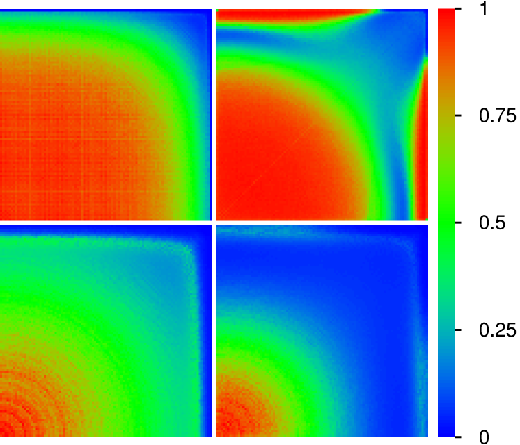
Figure 5: Phase diagram of the inverse participation ratio $\xi_{\rm IPR}$ in the plane of pair momentum ${\bf p}_{+}=(p_{+x},p_{+y})$ and computed from the same states, data and cases as in Fig. 4. The maximum values corresponding to the red region close to the bottom left corner ${\bf p}_{+}=(0,0)$ are $\xi_{\rm IPR}=15300$ (top left), $\xi_{\rm IPR}=4300$ (bottom left), $\xi_{\rm IPR}=18200$ (top right) and $\xi_{\rm IPR}=8600$ (bottom right). The minimum values at the top right corner ${\bf p}_{+}=(\pi,\pi)$ are $\xi_{\rm IPR}=14.87$ (top left), $\xi_{\rm IPR}=4$ (bottom left), $\xi_{\rm IPR}=126$ (top right) and $\xi_{\rm IPR}=9.8$ (bottom right). For comparison the ergodic value is $\xi_{\rm IPR,erg}=192^{2}=36864$ and the value for the totally symmetrized and localized initial state is $\xi_{\rm IPR,init}=4$.

The above observations are perfectly confirmed by the phase diagram for the inverse participation ratio $\xi_{\rm IPR}$ which is shown in Fig. 5 for the same cases and raw data of Fig. 4. Large (small) values of $\xi_{\rm IPR}$ corresponds to small (large) values of $w_{10}$ and a small (strong) pair formation probability. Here minimum (maximum) values are at ${\bf p}_{+}=(\pi,\pi)$ (${\bf p}_{+}=(0,0)$) as for the effective bandwidth of Fig. 1 (see figure caption for the numerical minimum, maximum and ergodic values). The boundary structure of the NN-model and the circle-structure of the HTC-case are also clearly visible.

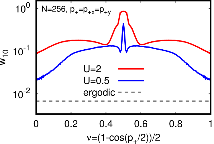
Figure 6: Dependence of the electron pair formation probability $w_{10}$ on $\nu=(1-\cos(p_{+}/2))/2$ for $p_{+}=p_{+x}=p_{+y}$ and the HTC-model at $U=0.5,\,2$ and $N=256$. $w_{10}$ is computed from the same long time average as in Fig. 4. The maximum value at $\nu=\nu_{\rm max}=0.5$ is $w_{10}=0.8535$ ($w_{10}=0.4456$) for $U=2$ ($U=0.5$). See Fig. 5 of [12] for the corresponding figure for the NN-model. For the NN-model the maximum value at $\nu=\nu_{\rm max}=0.5$ is exactly $w_{10}=1$ for both interaction values.

We have also computed the long time average of the pair formation probability for the HTC-model at larger system size $N=256$ and the special cases of either $p_{+x}=p_{+y}$ or $p_{+y}=0$ where the additional second symmetry (see discussion in the previous section and Appendix A) reduces the computational effort. In this way we can explore the diagonal and right boundary of the phase diagram in more detail.

Figure 6 shows $w_{10}$ for the HTC-model, $N=256$, $p_{+}=p_{+x}=p_{+y}$ and both interaction values $U=0.5,\,2$ as a function of the parameter $\nu=(1-\cos(p_{+}/2))/2$. Both curves clearly confirm some of the observations of the phase diagrams, i.e. strongest pair formation probability at $\nu=0.5$ ($p_{+x,y}=\pi$) with a somewhat larger maximum range for $U=2$ as compared to $U=0.5$ and a minimal pair formation probability at $\nu=0$ ($p_{+x,y}=0$) or $\nu=1$ ($p_{+x,y}=2\pi$) but still clearly above the ergodic limit for all cases. The precise numerical maximum values of $w_{10}$ at $\nu=0.5$ are slightly different from, but still in general agreement with, those of Fig. 4 due to the different system size. The corresponding figure for the NN-model was already given in [12].

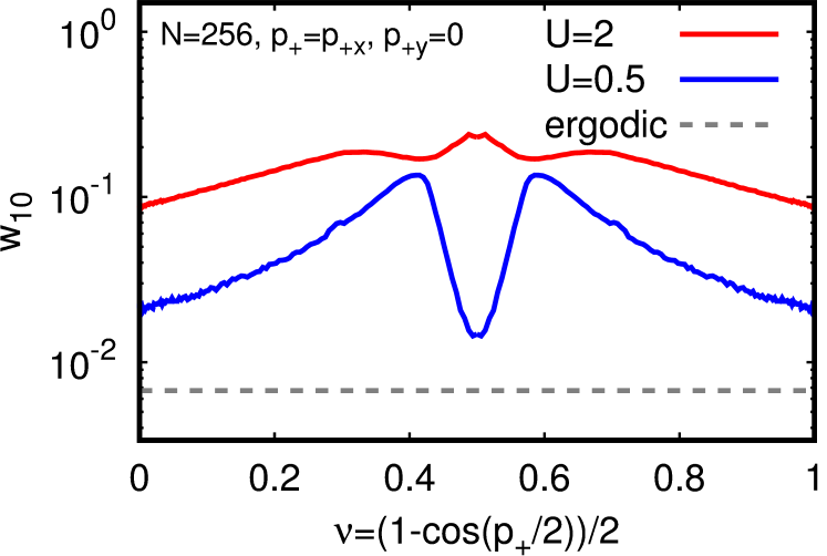
Figure 7: Dependence of the electron pair formation probability $w_{10}$ on $\nu=(1-\cos(p_{+}/2))/2$ for $p_{+}=p_{+x},p_{+y}=0$ and the HTC-model at $U=0.5,2$ and $N=256$. $w_{10}$ is computed from the same long time average as in Fig. 4. The value at $\nu=0.5$ is $w_{10}=0.2302$ ($w_{10}=0.01479$) for $U=2$ ($U=0.5$).

Figure 7 shows $w_{10}$ for the HTC model, $N=256$ and both interaction values $U=0.5,\,2$ at the boundary $p_{+y}=0$ as a function of the parameter $\nu=(1-\cos(p_{+}/2))/2$ with $p_{+}=p_{+x}$. The curve for $U=0.5$ clearly shows a strong local maximum at $\nu\approx 0.5\pm 0.1$ ($p_{+}\approx\pi\pm\pi/8$) corresponding to green-circle with radius $r_{g}\approx 0.85\pi$ visible in the phase diagram. For $U=2$ there are higher but less pronounced local maxima at $\nu\approx 0.5\pm 0.19$ corresponding to the slightly visible circle for this case. However, at $U=2$ the value of $w_{10}$ at $\nu=0.5$ is rather high while at $U=0.5$ its value at $\nu=0.5$ is quite low but still clearly above the ergodic limit.

Figures S1 and S2 of the supplementary material are similar to Figs. 6 and 7 respectively but for the inverse participation ratio $\xi_{\rm IPR}$.

6 Time evolution of pair formation

We also computed a more precise time evolution of the pair formation probability $w_{10}$ for the larger system size $N=384$ and certain specific cases $p_{+x}=p_{+y}\;\in\;\{0,\,2\pi/3,\,\pi\}$ and $p_{+y}=0$ with $p_{+x}\;\in\;\{7\pi/8,\,\pi\}$. The results together with the full space results using the Trotter formula approximation at $N=128$ are shown in Fig. 8 for $U=0.5,\,2$. In all cases the value of $w_{10}$ starts decaying from its initial value $w_{10}=1$ at $t/\Delta t>20$-$30$ and converges to a long time saturation value for $t/\Delta t>10^{3}$ sometimes with some temporal quasi-periodic fluctuations. In most cases the saturation values at $U=2$ are clearly larger than for $U=0.5$ except for the case $p_{+y}=0$ and $p_{+x}=7\pi/8$ where both saturation values are somewhat comparable. In particular, at $U=0.5$ the value for $p_{+y}=0$ and $p_{+x}=7\pi/8$ is significantly larger than the value for $p_{+y}=0$ and $p_{+x}=\pi$ while at $U=2$ it is the inverse. This observation is in agreement with the appearance of the green circle in the phase diagram where for $U=0.5$ the circle is dominant in comparison to the right boundary while for $U=2$ it is dominated by the right boundary.

The saturation value of the data obtained by the Trotter formula approximation, which somehow corresponds to an average over all possible ${\bf p}+$ values, is quite low if compared to the case ${\bf p}_{+}=0$ but still clearly above the corresponding ergodic value (for its reduced system size). Also for most of the other cases the saturation value is clearly above the ergodic value except for $U=0.5$, $p_{+y}=0$ and $p_{+x}=\pi$ where the curve is a $t\approx 10^{3}\Delta t$ even below the ergodic value and saturates later at a value only slightly above the ergodic value.

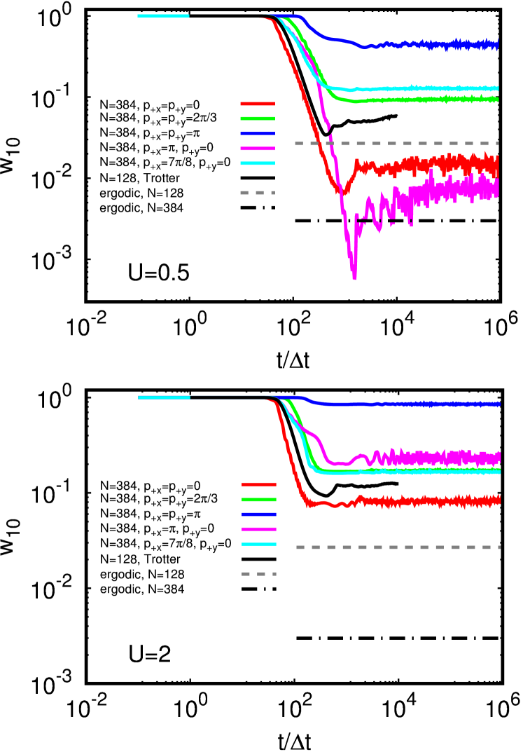
Figure 8: Time dependence of the pair formation probability $w_{10}$ for $U=0.5$ (top panel) and $U=2$ (bottom panel) and different cases of the exact time evolution in certain ${\bf p}_{+}=(p_{+x},p_{+y})$ sectors at $N=384$ and the full space Trotter formula time evolution at $N=128$. The dashed lines correspond to the ergodic values $(21/N)^{2}=0.0269$ for $N=128$ (grey dashed) and $(21/N)^{2}=0.00299$ for $N=384$ (black dashed).

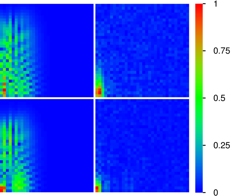
Figure 9: Color plot of wavefunction amplitude $|\bar{\psi}({\bf p}_{+},{\Delta{\bf r}})|$ in block representation in ${\Delta{\bf r}}=(\Delta x,\Delta y)$ plane obtained from the 2D quantum time evolution for the HTC lattice with $N=384$ and the sector $p_{+x}=7\pi/8$, $p_{+y}=0$. All panels show a zoomed region $0\leq\Delta x,\Delta y<32$. Left (right) panels correspond to $t=100\,\Delta t$ ($t=10^{5}\Delta t$; with $\Delta t=1/B_{2}=1/(16+U)$) and top (bottom) panels correspond to interaction strength $U=0.5$ ($U=2$). Related videos are available at [15].

Motivated by the observation of the green-circle at radius $r_{g}\approx 0.85\pi$ in the phase diagram for $U=0.5$, we show in Fig. 9 the wavefunction amplitude at $p_{+x}=7\pi/8$, $p_{+y}=0$, $N=384$ and both interaction values $U=0.5,\,2$ and two time values $t/\Delta t=100,\,10^{5}$. The first observation is that the diffusive spreading in $x$-direction is strongly suppressed if compared to the $y$-direction which is expected since $p_{+x}$ is rather close to $\pi$ while $p_{+y}=0$.

At $U=0.5$ the steady-state at $t/\Delta t=10^{5}$, despite a smaller value of $w_{10}=0.0754$ if compared to $w_{10}=0.1342$ at $U=2$, has a larger spatial extension of $\sim 30$ lattice sites compared to $\sim 12$ lattice sites for $U=2$. This in rough qualitative agreement with the values $\xi_{\rm IPR}=940$ (for $U=0.5$) and $\xi_{\rm IPR}=268$ (for $U=2$). However, a large amount of the contribution to the inverse participation ratio comes from the remaining probability of about 87-90% which has uniformly spread over the full lattice thus explaining the difference between $\xi_{\rm IPR}$ and the visible spatial extension in Fig. 9 (for this reason with consider $w_{10}$ to be a more suitable quantity than $\xi_{\rm IPR}$ to describe the pair formation probability).

7 Results overview

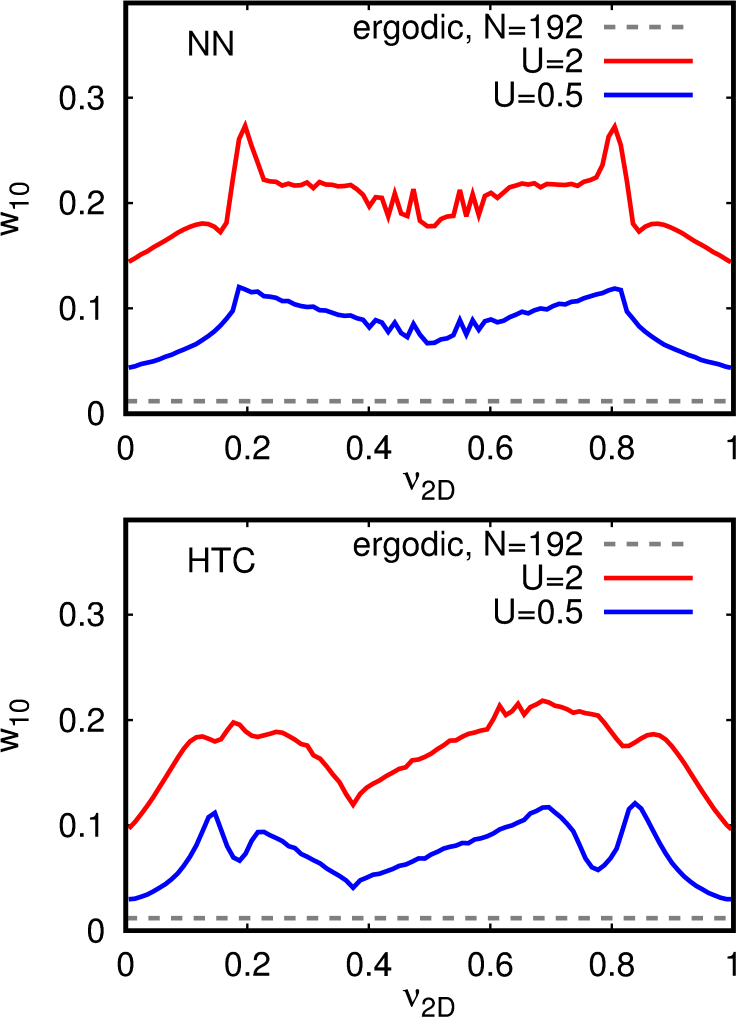
Figure 10: Dependence of the electron pair formation probability $w_{10}$ on the effective 2D filling factor $\nu_{2D}$ for the NN-lattice (top) and the HTC-lattice (bottom). The values of $w_{10}$ have been obtained from the data of Fig. 4 (for $N=192$) by an average along lines of constant electron pair energy $E_{c}$ at momenta ${\bf p}_{1}={\bf p}_{2}={\bf p}_{+}/2$ with $p_{+x},\,p_{+y}\in[0,2\pi]$. Lowest (largest) energy corresponds to $\nu_{2D}=0$ ($\nu_{2D}=1$). The data points shown correspond to an effective histogram with bin width $\Delta\nu_{2D}\approx 0.01$. The red (blue) curve corresponds to the interaction value $U=2$ ($U=0.5$) and the grey dashed line corresponds to the ergodic value $(21/192)^{2}=0.01196$.

The discussion of the phase diagram given in Fig. 4 has shown that the pair formation probability is maximal at the point ${\bf p}_{+}=(\pi,\pi)$. However, the surrounding region to this point is quite small if compared to the green-circle where we have a somewhat more modest pair formation probability. In terms of available values of ${\bf p}_{+}$ the latter region is possibly more important. In order to analyze this point in a more quantitative way, we assume a simple model where both electrons have the same momentum ${\bf p}_{+}/2$ (i.e. $\Delta p=0$) and where the available states of this type are filled from smallest to largest energies. We subdivide these states, ordered in energy, in slices of equal number ($\sim 1/100$ of all available states) and compute the average of $w_{10}$ for each slice which is equivalent to the average of $w_{10}$ at lines of constant energy. In Fig.10, we show the dependence of this average on the effective 2D-filling factor $\nu_{2D}$ which is the weight of slices below a certain energy.

For the NN-model we observe a strong peak at $\nu_{2D}=0.2$ (and similarly at $\nu_{2D}=0.8$ due to symmetry). This peak is caused by the combination of the maximum point at ${\bf p}_{+}=(\pi,\pi)$ and rather strong (top or right) boundary contributions visible in the left panels of Fig. 4. For the HTC-model at $U=2$ this peak is still visible but its value is reduced. However, for $U=0.5$, there are two separated peaks, a stronger one at $\nu_{2D}\approx 0.15$ related to the average over the green circle at radius $r_{g}\approx 0.85$ and a second lower peak at $\nu_{2D}\approx 0.24$ related to the average of the maximum region close to ${\bf p}_{+}=(\pi,\pi)$. For this particular case, the green circle has a stronger global contribution to the pair formation probability than the maximum region at ${\bf p}_{+}=(\pi,\pi)$.

8 Discussion

In our studies we analyzed the electron pair formation in a tight-binding model of La-based cuprate superconductors induced by Coulomb repulsion. Our analytical and numerical results show that even a repulsive Coulomb interaction can form two electron pairs with a high probability. Such pairs have a compact size and propagate through the whole system. We expect that such pairs may contribute to the emergence of superconductivity in La-based cuprates.

Of course, our analysis only considers two electrons and in a real system at finite electron density there is a Fermi sea which can modify electron interactions. However, we expect that electrons significantly below the Fermi energy will only create a mean-field potential which will not significantly affect interacting electrons with energies in the vicinity of the Fermi energy. A detailed investigation of effects of finite electron density on the Coulomb pair formation represents an important task for future studies.

9 Acknowledgments

This work has been partially supported through the grant NANOX $N^{o}$ ANR-17-EURE-0009 in the framework of the Programme Investissements d’Avenir (project MTDINA). This work was granted access to the HPC resources of CALMIP (Toulouse) under the allocation 2020-P0110.

Appendix A Appendix

In this appendix we present the derivation of the block Hamiltonian (11) and a more detailed discussion about its discrete symmetries. In order to simplify the notations, we will use here the full set ${\cal A}^{\prime}={\cal A}\cup(-{\cal A})$ of neighbor vectors (in the full and not only half plane) for the summation over the vectors ${\bf a}$ which allows to reduce the number of terms in the following expressions. The TIP Hamiltonian (5) can then be written in a more explicit form as:

$$H = -\sum_{{\bf r}_{1},{\bf r}_{2}}\sum_{{\bf a}\in{\cal A}^{\prime}}t_{\bf a}\bigl{(}|{\bf r}_{1},{\bf r}_{2}\rangle\langle{\bf r}_{1}+{\bf a},{\bf r}_{2}|+|{\bf r}_{1},{\bf r}_{2}\rangle\langle{\bf r}_{1},{\bf r}_{2}-{\bf a}|\bigr{)}$$ (13)

$$+\sum_{{\bf r}_{1},{\bf r}_{2}}\bar{U}({\bf r}_{2}-{\bf r}_{1})|{\bf r}_{1},{\bf r}_{2}\rangle\langle{\bf r}_{1},{\bf r}_{2}|$$

where for convenience we have written “${\bf r}_{2}-{\bf a}$” instead of “${\bf r}_{2}+{\bf a}$” (in the second term of the first line) since for ${\bf a}\in{\cal A}^{\prime}$ also $-{\bf a}\in{\cal A}^{\prime}$. Furthermore, the terms with shifts of ${\bf a}$ in the left side have been absorbed by the increased set ${\cal A}^{\prime}$ (with respect to ${\cal A}$ used in (1)) combined with a subsequent shift of the summation index ${\bf r}_{1}$ or ${\bf r}_{2}$ and exploiting the periodic boundary conditions.

Applying (13) to a block basis state (10) we find that:

$$H|{\bf p}_{+},{\Delta{\bf r}}\rangle = -\frac{1}{N}\sum_{{\bf r}_{1}}\sum_{{\bf a}\in{\cal A}^{\prime}}t_{\bf a}\Bigl{(}|{\bf r}_{1}-{\bf a},{\bf r}_{1}+{\Delta{\bf r}}\rangle\,e^{i{\bf p}_{+}\cdot({\bf r}_{1}+{\Delta{\bf r}}/2)}$$

$$+|{\bf r}_{1},{\bf r}_{1}+{\Delta{\bf r}}+{\bf a}\rangle\,e^{i{\bf p}_{+}\cdot({\bf r}_{1}+{\Delta{\bf r}}/2)}\Bigr{)}$$

$$+\bar{U}({\Delta{\bf r}})|{\bf p}_{+},{\Delta{\bf r}}\rangle.$$

Using the shift ${\bf r}_{1}\to{\bf r}_{1}+{\bf a}$ in the ${\bf r}_{1}$-sum of the first line of this expression we obtain:

$$H|{\bf p}_{+},{\Delta{\bf r}}\rangle = -\frac{1}{N}\sum_{{\bf r}_{1}}\sum_{{\bf a}\in{\cal A}^{\prime}}t_{\bf a}\Bigl{(}|{\bf r}_{1},{\bf r}_{1}+{\Delta{\bf r}}+{\bf a}\rangle\,e^{i{\bf p}_{+}\cdot({\bf r}_{1}+{\bf a}+{\Delta{\bf r}}/2)}$$

$$+|{\bf r}_{1},{\bf r}_{1}+{\Delta{\bf r}}+{\bf a}\rangle\,e^{i{\bf p}_{+}\cdot({\bf r}_{1}+{\Delta{\bf r}}/2)}\Bigr{)}$$

$$+\bar{U}({\Delta{\bf r}})|{\bf p}_{+},{\Delta{\bf r}}\rangle$$

which can be rewritten as:

$$H|{\bf p}_{+},{\Delta{\bf r}}\rangle = -\frac{1}{N}\sum_{{\bf r}_{1}}\sum_{{\bf a}\in{\cal A}^{\prime}}t_{\bf a}\,|{\bf r}_{1},{\bf r}_{1}+{\Delta{\bf r}}+{\bf a}\rangle$$ (16)

$$\qquad\times\,e^{i{\bf p}_{+}\cdot[{\bf r}_{1}+({\Delta{\bf r}}+{\bf a})/2]}\underbrace{\left(e^{i{\bf p}_{+}\cdot{\bf a}/2}+e^{-i{\bf p}_{+}\cdot{\bf a}/2}\right)}_{2\cos({\bf p}_{+}\cdot{\bf a}/2)}$$

$$+\bar{U}({\Delta{\bf r}})|{\bf p}_{+},{\Delta{\bf r}}\rangle$$

$$= -2\sum_{{\bf a}\in{\cal A}^{\prime}}t_{\bf a}\,\cos({\bf p}_{+}\cdot{\bf a}/2)\,|{\bf p}_{+},{\Delta{\bf r}}+{\bf a}\rangle$$

$$+\bar{U}({\Delta{\bf r}})|{\bf p}_{+},{\Delta{\bf r}}\rangle\ .$$

The last expression provides exactly the effective block Hamiltonian (11) if we replace the sum over ${\bf a}\in{\cal A}^{\prime}$ by a sum over ${\bf a}\in{\cal A}$ with two contributions “$+{\bf a}$” and “$-{\bf a}$” and applying for the latter contribution a subsequent shift ${\Delta{\bf r}}\to{\Delta{\bf r}}+{\bf a}$ in the ${\Delta{\bf r}}$ sum. However, there is one additional complication if ${\Delta{\bf r}}+{\bf a}=(\Delta x+a_{x},\Delta y+a_{y})$ in (A) leaves the initial square of $\Delta x,\Delta y\in\{0,\ldots N-1\}$. Then we have to add (subtract) $N$ to (from) $\Delta x+a_{x}$ and/or $\Delta y+a_{y}$ which provides according to (10) the factor $e^{\pm ip_{+x}N/2}=e^{\pm i\pi l_{+x}}=(-1)^{l_{+x}}$ (for $\Delta x$ and similarly for $\Delta y$) resulting in either periodic or anti-periodic boundary conditions in $x$- ($y$-)direction depending on the parity of the integer index $l_{+x}$ ($l_{+y}$).

We close this appendix with a short discussion about the discrete reflection symmetries of the block Hamiltonian (11) and the possibility to reduce its effective matrix size $N^{2}$ due to such symmetries. For the NN-model, as already discussed in detail in [12], there are at least two symmetries with respect to $\Delta x\to N-\Delta x$ (reflection at the $\Delta y$-axis) or $\Delta y\to N-\Delta y$ (reflection at the $\Delta x$-axis) and in case if $p_{+x}=p_{+y}$ there is a third symmetry with respect to $\Delta x\leftrightarrow\Delta y$ (reflection at the $\Delta x$-$\Delta y$ diagonal) which allows for an effective matrix size of roughly either $N^{2}/4$ or $N^{2}/8$ (if $p_{+x}=p_{+y}$).

However, for a more general lattice, such as the HTC-model, or more generally in presence of at least one neighbor vector ${\bf a}=(a_{x},a_{y})$ with both $a_{x}\neq 0$ and $a_{y}\neq 0$ (e.g. ${\bf a}=(1,1)$) the number of symmetries is reduced. For the most generic case with $p_{+x}\neq p_{+y}$, $p_{+x}\neq 0$ and $p_{+y}\neq 0$ there is only one symmetry corresponding to particle exchange with two simultaneous transformations $\Delta x\to N-\Delta x$ and $\Delta y\to N-\Delta y$ which allows for a reduction of the effective matrix size to $\approx N^{2}/2$. In this case the factors $\cos({\bf p}_{+}\cdot{\bf a}/2)=\cos[(p_{+x}a_{x}+p_{+y}a_{y})/2]$ appearing in the effective hopping amplitudes are not modified because the replacement ${\bf a}\to-{\bf a}$ due the symmetry transformation only changes the global sign inside the cosine argument. However, this is no longer true if we apply for example the transformation $\Delta x\to N-\Delta x$ without modifying $\Delta y$ which is equivalent to the replacement of $(a_{x},a_{y})\to(-a_{x},a_{y})$ of the neighbor vectors. Therefore a single reflection at the $\Delta y$ (or $\Delta x$) axis modifies the hopping amplitude (if both $a_{x}\neq 0$, $a_{y}\neq 0$ and also both $p_{+x}\neq 0$, $p_{+y}\neq 0$) and (11) is (in general) not invariant with respect to such transformations. However, if either $p_{+x}=0$ or $p_{+y}=0$ the effective hopping amplitudes are not modified with respect to these two individual reflections and we have two symmetries with an effective matrix size of $\approx N^{2}/4$. Also if $p_{+x}=p_{+y}\neq 0$ we have two symmetries (particle exchange and reflection at the $\Delta x$-$\Delta y$ diagonal) leading also to an effective matrix size of $\approx N^{2}/4$. Finally, for the special case $p_{+x}=p_{+y}=0$, we have even three symmetries (as in the NN-Model for $p_{+x}=p_{+y}$) with effective matrix size of $\approx N^{2}/8$.

Supplementary Material for
Coulomb electron pairing in a tight-binding model of La-based cuprate superconductors
by K. M. Frahm and D. L. Shepelyansky.

Here, we present additional material for the main part of the article.

Figure S1 presents data for the inverse participation ratio for the case of Fig. 6.

Figure S2 presents data for the inverse participation ratio for the case of Fig. 7.

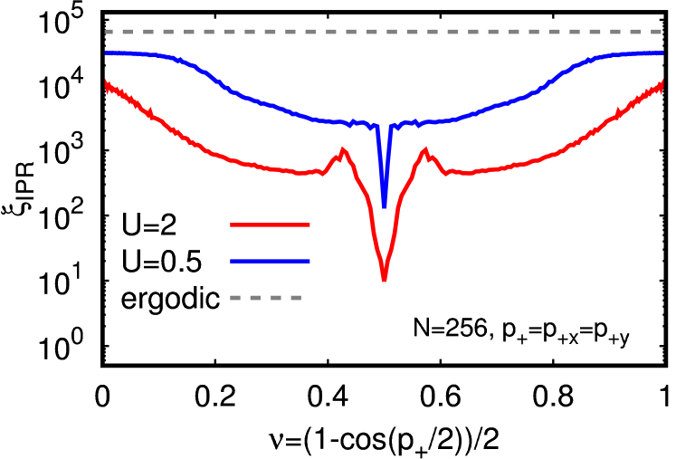
Figure S1: As Fig. 6 but for the inverse participation ratio $\xi_{\rm IPR}$.

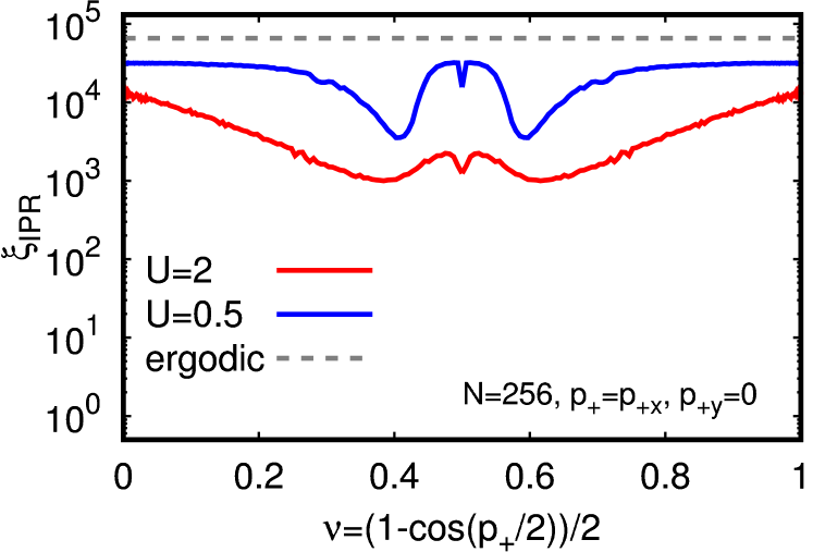
Figure S2: As Fig. 7 but for the inverse participation ratio $\xi_{\rm IPR}$.

Two video files for the time evolution obtained by the Trotter formula approximation corresponding to the parameters of Fig. 2 and Fig. 3 are presented in files videofig2.avi for the density $\rho_{XX}(x_{1},x_{2})$ defined in Eq. (8) and in videofig3.avi for the density $\rho_{\rm rel}(\Delta x,\Delta y)$ defined in Eq. (9) (here $N=128$, $U=2$). Both video files provide a direct comparison between the NN-model (right box in video) and the HTC-model (left box in video) and correspond to 464 time values $t=l_{j}\,\Delta t$ (25 values per second of video) with integer $l_{0}=0$, $1\leq l_{j}\leq 10^{4}$ for $j=1,\ldots,463$ and roughly uniform logarithmic density.

References

- [1] K. A. Müller, J. G. Bednorz, \jrZ. Phys. B: Condens. Matter 1986, 64, 189.
- [2] E. Dagotto, \jrRev. Mod. Phys. 1994, 66, 763.
- [3] B. Keimer, S. A. Kivelson, M. R. Norman, S. Uchida, Z. Zaanen, \jrNature 2015, 518, 179.
- [4] C. Proust, L. Taillefer, \jrAnnu. Rev. Condens. Matter Phys. 2019, 10, 409.
- [5] P. W. Anderson, \jrScience 1987, 235, 1196.
- [6] R. Photopoulos, R. Fresard, \jrAnn. Phys. (Berlin) 2019, 1900177.
- [7] V. J. Emery, \jrPhys. Rev. Lett. 1987, 58, 2794.
- [8] V. J. Emery, G. Reiter, \jrPhys. Rev. B 1988, 38, 4547.
- [9] C. M. Varma, \jrSolid State Commun. 1987, 62, 681.
- [10] Y. B. Gaididei, V. M. Loktev, \jrPhys. Status Solidi 1988, 147, 307.
- [11] R. S. Markiewicz, S. Sahrakorpi, M. Lindroos, H. Lin, A. Bansil, \jrPhys. Rev. B 2005, 72, 054519.
- [12] K. M. Frahm, D. L. Shepelyansky, \jrPhys. Rev. Research 2020, 2, 023354.
- [13] K. M. Frahm, D. L. Shepelyansky, \jrEur. Phys. J. B 2016, 89, 8.
- [14] See Supplemental Material at http:XXXX that contains extra-figures and videos supporting the main conclusions and results.
- [15] K. M. Frahm, D. L. Shepelyansky, Available upon request: http://www.quantware.ups-tlse.fr/QWLIB/ectronpairsforhtc/; Accessed July (2020)