A NEW APPROACH TO FIND AN APPROXIMATE SOLUTION OF LINEAR INITIAL VALUE PROBLEMS

Abstract

This work investigates a new approach to find closed form analytical approximate solution of linear initial value problems. Classical Bernoulli polynomials have been used to derive a finite set of orthonormal polynomials and a finite operational matrix to simplify derivatives of dependent variable. These orthonormal polynomials together with the operational matrix of relevant order provides a good approximation to the solution of a linear initial value problem. Depending upon the nature of a problem, a series form approximation or numerical approximation can be obtained. The technique has been demonstrated through three problems. Approximate solutions have been compared with available exact or other numerical solutions. High degree of accuracy has been noted in numerical values of solutions for considered problems.

1 Introduction

Initial value problems (IVPs) for ordinary differential equations arise in a natural way in real life problems and modelling of science and engineering problems. Some examples of such modelling problems are heat conduction, wave propagation, diffusion problems, gas dynamics, nuclear physics, atomic structures, fluid flow and chemical reactions, continuum mechanics, electricity and magnetism, geophysics, antenna, synthesis problem, population genetics communication theory, mathematical modelling of economics, radiation problems and astrophysics. Many times, the exact analytic solution of such problems are not available which give rise a need to find numerical solutions. Bulk of literature is available to explore exact and numerical solutions of initial and boundary value problems [1, 2, 3, 4]. Many researchers have focused their attention to find approximate solutions differential and integral equations. Xu [5] adopted method of variational iteration, Pandey, et. al. [6] applied homotopic perturbation and method of collocation. Cheon [7] discussed possible applications of Bernoulli polynomials and functions in numerical analysis. Some other latest investigations include uses of Chebyshev polynomials [8], Legendre polynomials [9], Laguerre polynomials and Wavelet Galerkin method [10], Legendre wavelets [11], the operational matrix [12].

Numerical solution to boundary value problems has been also presented by Shiralashetti and Kumbinarasaiah [13, 14], Abd-Elhameed et al. [15], Iqbal et al. [16] and, Kumar and Singh [17]. Bernoulli polynomials and its properties have been also discussed by many authors [18, 19]. Tohidi et. al. [20] obtained numerical approximation for generalized pantograph equation using Bernoulli matrix method, Tohidi and Khorsand [21] to solve second-order linear system of partial differential equations, Mohsenyzadeh [22] used Bernoulli polynomials to solve Volterra type integral equations. Recently, Singh et al. [23] used Bernoulli polynomials to develop a trigonal operational matrix to solve Abel-Volterra type integral equations.

In this work, it is proposed to solve linear initial value problems using orthogonal polynomials derived from Bernoulli polynomials with a modified operational matrix [23].

2 Bernoulli Polynomials

The word Bernoulli Polynomials was first coined by J. L. Raabe in 1851 while discussing the formula $\sum\limits_{n=0}^{m-1}{{B_{n}}\left({x+\frac{k}{m}}\right)}={m^{-(n+1)}}{B_{n}}(mx)$, however, the polynomials $B_{n}(x)$ were already introduced by Jakob Bernoulli in 1690 in his book ”$ArsConjectandi$” [24]. A thorough study of these polynomials was first done by Leonhard Euler in 1755, who showed in his book “Foundations of differential calculus” that these polynomials satisfy the finite difference relation:

$${B_{n}}(\zeta+1)-{B_{n}}(\zeta)=n{\zeta^{n-1}},\,\,\,\,\,n\geq 1$$ (1)

and proposed the method of generating function to calculate $B_{n}(x)$. Following Leonhard Euler, recently Costabile and Dell’Accio [24] showed that Bernoulli Polynomials are monic which can be extracted from its generating function

$$\frac{{\gamma\,{e^{\zeta\gamma}}}}{{{e^{\gamma}}-1}}=\sum\limits_{n=0}^{\infty}{{B_{n}}(\zeta)\,\frac{{{\gamma^{n}}}}{{n!}}}\,\,\,\,\,\left({\left|\zeta\right|<2\pi}\right)$$ (2)

and represented in the simple form:

$${B_{n}}(\zeta)=\sum\limits_{j=0}^{n}{\,\left({\begin{array}[]{*{20}{c}}n\\ j\end{array}}\right)\,\,{B_{j}}(0)\,{\zeta^{n-j}},\hskip 10.00002ptn=0,1,2,...}\hskip 10.00002pt0\leq\zeta\leq 1$$ (3)

where, $B_{n}(0)$ are the Bernoulli numbers, which can also be calculated with Kronecker’s formula ${B_{n}}(0)=-\sum\limits_{j=1}^{n+1}{\frac{{{{(-1)}^{j}}}}{j}\left({\begin{array}[]{*{20}{c}}{n+1}\\ j\end{array}}\right)}\sum\limits_{k=1}^{j}{{k^{n}}}\,\,;\,\,\,n\geq 0$ [25]. Thus, first few Bernoulli polynomials can be written as ${B_{0}}(\zeta)=1,B_{1}(\zeta)=\zeta-\frac{1}{2},B_{2}(\zeta)=\zeta^{2}-\zeta+\frac{1}{6},B_{3}(\zeta)=\zeta^{3}-\frac{3}{2}\zeta^{2}+\frac{1}{2}\zeta,B_{4}(\zeta)=\zeta^{4}-2\zeta^{3}+\zeta^{2}-\frac{1}{30}$.

These Bernoulli Polynomials form a complete basis over $[0,1]$ [26] and show some interesting properties [27, 28]:

$$\left.\begin{gathered}B^{\prime}_{n}(\zeta)=n{B_{n-1}}(\zeta),\,\,\,n\geq 1\hfill\\ \int_{0}^{1}{{B_{n}}(z)dz=0,\,\,\,\,\,\,\,\,\,\,n\geq 1}\hfill\\ {B_{n}}(\zeta+1)-{B_{n}}(\zeta)=n{\zeta^{n-1}},\,\,n\geq 1\hfill\\ \end{gathered}\right\}.$$ (4)

3 The Orthonormal Polynomials

It can be easily verified that the polynomials ${B_{n}}(x)\,(n\geq 1)$ given by (eq.3) are orthogonal to $B_{o}(x)$ with respect to standard inner product on ${L^{2}}\in[0,1]$. Using this property, an orthonormal set of polynomials can be derived for any $n$ with Gram-Schmidt orthogonalization. First ten such orthonormal polynomials are obtained in A.

4 Approximation of Functions

Theorem. Let $H=L^{2}[0,1]$ be a Hilbert space and $Y=span\left\{y_{0},y_{1},y_{2},...,y_{n}\right\}$ be a subspace of $H$ such that $dim{(}Y)<\infty$ , every $f\in H$ has a unique best approximation out of $Y$ [26], that is, $\forall y(t)\in Y,\,\exists\,\hat{f}(t)\in Y$ s.t. $\parallel f(t)-\hat{f}(t)\parallel_{2}\leq\parallel f(t)-y(t)\parallel_{2}$. This implies that, $\forall\,y(t)\in Y,<f(t)-f(t),y(t)>=0$, where $<,>$ is standard inner product on $L^{2}\in[0,1]$ (c.f. Theorems 6.1-1 and 6.2-5, Chapter 6 [26]).

Remark. Let $Y=span\left\{\phi_{0},\phi_{1},\phi_{2},...,\phi_{n}\right\},$ where $\phi_{k}\in L^{2}[0,1]$ are orthonormal Bernoulli polynomials. Then, from the above theorem, for any function $f\in L^{2}[0,1],$

$$f\approx\hat{f}=\sum_{k=0}^{n}{c_{k}\phi_{k}},$$ (5)

where $c_{k}=\left\langle f,\phi_{k}\right\rangle,$ and $<,>$ is the standard inner product on $L^{2}\in[0,1]$. For numerical approximation, series (5) can be written as:

$$f(\zeta)\simeq\sum_{k=0}^{n}{c_{k}\phi_{k}=C^{T}\phi(\zeta)}$$ (6)

where $C=\left(c_{0},c_{1},c_{2},...,c_{n}\right),\phi(\zeta)=\left(\phi_{0},\phi_{1},\phi_{2},...,\phi_{n}\right)$ are column vectors, and number of polynomials $n$ can be chosen to meet required accuracy.

5 Construction of operational matrix

The orthonormal polynomials, as derived in A, can be expressed as:

$$\int_{0}^{\zeta}{{\phi_{o}}(\eta)d\eta}={\phi_{o}}(\zeta)+\frac{1}{{2\sqrt{3}}}{\phi_{1}}(\zeta)$$ (7)

$$\begin{array}[]{l}\int\limits_{0}^{\zeta}{{\phi_{i}}(x)dx=}\,\,\,\,\,\frac{1}{{2\sqrt{(2i-1)(2i+1)}}}{\phi_{i-1}}(\zeta)\\ \hskip 56.9055pt+\frac{1}{{2\sqrt{(2i+1)(2i+3)}}}{\phi_{i+1}}(\zeta),\,\,\,\,(\,for{\rm{}}\,i=1\,,2,...\,,n)\end{array}$$ (8)

Relations (7-8) can be represented in closed form as:

$$\int\limits_{0}^{\zeta}{\phi(\eta)d\eta=\,\,}\Theta\,\phi(\zeta)$$ (9)

where $\zeta\in[0,1]$ and $\Theta$ is operational matrix of order $(n+1)$ given as :

$$\Theta\,=\frac{1}{2}\left[{\begin{array}[]{*{20}{c}}1&{\frac{1}{{\sqrt{1.3}}}}&0&\cdots&0\\ {-\frac{1}{{\sqrt{1.3}}}}&0&{\frac{1}{{\sqrt{3.5}}}}&\cdots&0\\ 0&{-\frac{1}{{\sqrt{3.5}}}}&0&\ddots&\vdots\\ \vdots&\vdots&\ddots&\ddots&{\frac{1}{{\sqrt{\left({2n-1}\right)\left({2n+1}\right)}}}}\\ 0&0&\cdots&{-\frac{1}{{\sqrt{\left({2n-1}\right)\left({2n+1}\right)}}}}&0\end{array}}\right]$$ (10)

6 Solution of Initial Value Problems

Consider the linear IVP:

$$\frac{{{d^{2}}y}}{{d{\zeta^{2}}}}+P(\zeta)\frac{{dy}}{{d\zeta}}+Q(\zeta)y=r(\zeta),\,\,\,y(0)=\alpha,\left(\frac{dy}{d\zeta}\right)_{\zeta=0}=\beta$$ (11)

where $y=y(\zeta);p(\zeta)$ and $q(\zeta)$ and $r(\zeta)$ are continuous functions defined $[0,1]$. It is further assumed that eq. (11) admits a unique solution on $[0,1]$, otherwise, a suitable transformation $z=z(x)$ may be applied to change the domain of $y,p,q$ and $r$.

6.1 Case 1 : Coefficients of $y$ and $\frac{dy}{d\zeta}$ are constant

In this case, taking $p$ for $P(x)$ and $q$ for $Q(x)$, eq. (11), is written as:

$$\frac{{{d^{2}}y}}{{d{\zeta^{2}}}}+p\frac{{dy}}{{d\zeta}}+q(\zeta)y=r(\zeta),\,\,\,y(0)=\alpha,\left(\frac{dy}{d\zeta}\right)_{\zeta=0}=\beta$$ (12)

Let $R=\left(r_{o},r_{1},...,r_{n}\right)$ be a real column vector such that the function $r(\zeta)$ can be approximated in terms of first $n+1$ orthonormal Bernoulli polynomials as:

$$r\left(\zeta\right)=R\,\phi(\zeta)$$ (13)

Let $C=\left(c_{o},c_{1},c_{2},...,c_{n}\right)-$ be a column vector of $n+1$ unknown quantities. Taking

$$\frac{{{d^{2}}y}}{{d{\zeta^{2}}}}=C^{T}\,\phi(\zeta)$$ (14)

eq. (11) can be re-written as:

$${C^{T}}{\phi}(\zeta)+\,\,p\,\,{C^{T}}\,\Theta\,{\phi}(\zeta)+\,\,q\,\,{C^{T}}\,{\Theta^{2}}\,{\phi}(\zeta)=R^{T}\,{\phi}(\zeta)$$ (15)

which gives,

$$C^{T}\,\,={\left[{I+p\,\,\Theta+q\,\,{\Theta^{2}}}\right]^{-1}}\,R^{T}$$ (16)

Substituting eq. (16) back into eq. (14), an approximation for $y(\zeta)$ can be obtained as:

$$y(\zeta)={C^{T}}\,\Theta^{2}\,{\phi}(\zeta).$$ (17)

6.2 Case 2 : Coefficients of $y$ and $\frac{dy}{d\zeta}$ are functions of independent variable

Taking $P(\zeta)=a^{T}\phi(\zeta)$ and $Q(\zeta)=b^{T}\phi(\zeta)$ together with eqs. (13-14), eq. (11) can be written as:

$${C^{T}}{\phi}(\zeta)+\left(a^{T}\phi(\zeta)\right)\left(C^{T}\Theta\phi(\zeta)\right)+\left(b^{T}\phi(\zeta)\right)\left(C^{T}\Theta^{2}\phi(\zeta)\right)=R^{T}\,{\phi}(\zeta)$$ (18)

Because $a^{T}\phi(\zeta)$ and $b^{T}\phi(\zeta)$ in second and third terms respectively on left side of eq. (18) are just the polynomials or degree $2n$, eq. (18) can be re-written as,

$${C^{T}}{\phi}(\zeta)+C^{T}\Theta\left[\phi(\zeta)\left(a^{T}\phi(\zeta)\right)\right]+C^{T}\Theta^{2}\left[\phi(\zeta)\left(b^{T}\phi(\zeta)\right)\right]=R^{T}\,{\phi}(\zeta)$$ (19)

Here, $\phi(\zeta)\left(a^{T}\phi(\zeta)\right)$ is a vector of type

$$\left(\phi_{o}(\zeta)\sum_{k=0}^{k=n}a_{k}\phi_{k}(\zeta),\,\phi_{1}(\zeta)\sum_{k=0}^{k=n}a_{k}\phi_{k}(\zeta),\,\dots,\,\phi_{n}(\zeta)\sum_{k=0}^{k=n}a_{k}\phi_{k}(\zeta)\right)$$

$$\equiv(\psi_{o}(\zeta),\psi_{1}(\zeta),\dots,\psi_{n}(\zeta))=\psi(\zeta),\hskip 14.22636pt(say!)$$ (20)

In eq. (20), each $\psi_{k}(\zeta)$ can be approximated as a linear combination of orthonormal polynomials in the form $\psi_{k}(\zeta)=A_{k}^{T}\phi(\zeta)$, where $A_{k}^{T}$ are vectors of form $1\times(n+1)$ for $k=1,2,\dots,n$, and, therefore, $\phi(\zeta)\left(a^{T}\phi(\zeta)\right)=\psi(\zeta)=A\phi(\zeta)$, where $A=\left(A_{o}^{T},A_{1}^{T},\dots,A_{n}^{T}\right)_{(\underline{n+1}\times 1)}$. Similarly, $\phi(\zeta)\left(b^{T}\phi(\zeta)\right)$ can be approximated as $B^{T}\phi(\zeta)$ for some vector $B^{T}=(B_{o},B_{1},\dots,B_{n})_{(\underline{n+1}\times 1)}$ such that $B_{k}^{T}$ are real vectors of form $1\times(n+1)$. With these intermediate approximations, eq. (19) can be written as :

$${C^{T}}{\phi}(\zeta)+C^{T}\Theta A\phi(\zeta)+C^{T}\Theta^{2}B\phi(\zeta)=R^{T}\,{\phi}(\zeta)$$ (21)

From eq. (21), the required coefficient vector $C$ is obtained as:

$$C^{T}=R^{T}\left(I+\theta A+\theta^{2}B\right)^{-1},$$ (22)

where, $I$ is identity matrix of order $n$. The expression for $y(\zeta)$ is obtained as:

$$y(\zeta)={C^{T}}\,\Theta^{2}\,{\phi}(\zeta)$$ (23)

7 Numerical Examples

In order to discuss and establish the accuracy and efficacy of the present method, following examples have been taken.

Example 1:

Let us consider the IVP

$$\frac{d^{2}y}{dx^{2}}+5\frac{dy}{dx}+3y=e^{-x};\hskip 10.00002pty(0)=\left(\frac{dy}{dx}\right)_{x=0}=0$$ (24)

which has exact solution $y(x)=e^{-\frac{5}{2}x}\left(\cosh(\frac{\sqrt{13}}{2}x)+\frac{3}{\sqrt{13}}\sinh(\frac{\sqrt{13}}{2}x)\right)-e^{-x}$.

Comparing eq.(24) with eq. (11) and taking $m=6$, equations (13 - 16) yield

$${B^{T}}=\left(\begin{array}[]{cccc}0.08086,&-0.02459,&-0.00156,&-0.00240,\\ -0.001046,&-0.000425,&-0.00017,&0\end{array}\right)$$ (25)

Using value of $B^{T}$ in eq. (17), an approximate solution is obtained as:

$$y(x)\approx-0.00009x+0.25057x^{2}-0.08655x^{3}+0.07415x^{4}$$

$$-0.10716x^{5}+0.0930x^{6}-0.03382x^{7}$$ (26)

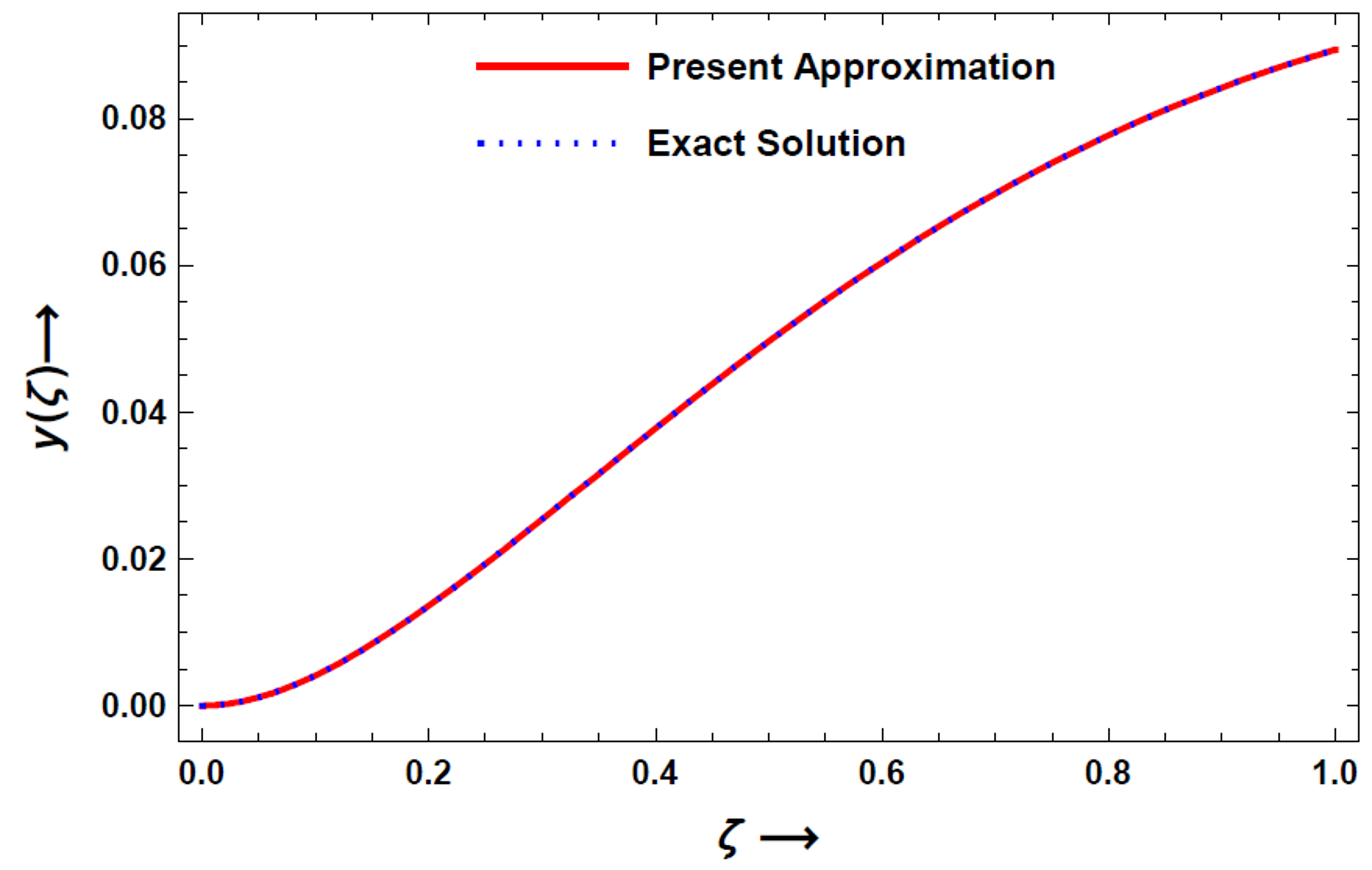
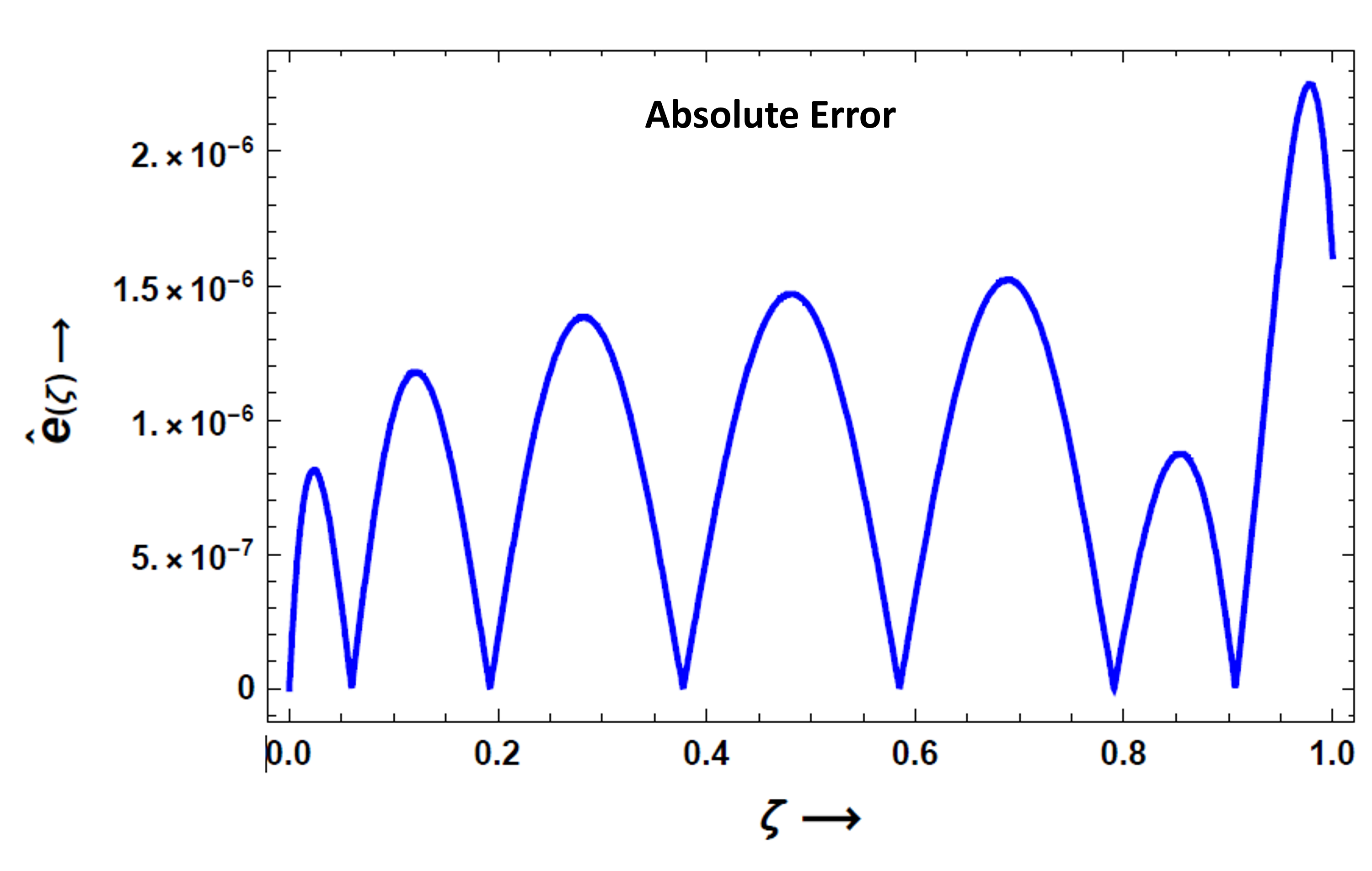
(a)                                                             (b)

Figure 1: (a) Comparison of exact and present solution for example 1. (b) Absolute error between exact and approximate solutions of example 1

Example 2:

Consider the IVP

$$\frac{d^{2}y}{dx^{2}}-5\frac{dy}{dx}+2y=\tan(x);\hskip 10.00002pty(0)=\left(\frac{dy}{dx}\right)_{x=0}=0$$ (27)

which is linear in nature but its not easy to solve manually. We will compare the present solution of this IVP with the one generated by Mathematica.

Comparing eq.(27) with eq. (11) and taking $m=9$, equations (13 - 16) yield

$${B^{T}}=\left(\begin{array}[]{c}5.1220,\,\,5.5181,\,\,2.9304,\,\,1.0668,\,\,0.2958,\\ 0.0663,\,\,0.0125,\,\,0.0020,\,\,0.0003,\,\,0,\,\,0\end{array}\right)$$ (28)

Using value of $B^{T}$ in eq. (17), an approximate solution is obtained as:

$$y(x)\approx 0.0001x-0.0025x^{2}+0.1942x^{3}+0.04799x^{4}+0.7521x^{5}$$

$$-0.9599x^{6}+1.5043x^{7}-0.9351x^{8}+0.3669x^{9}$$ (29)

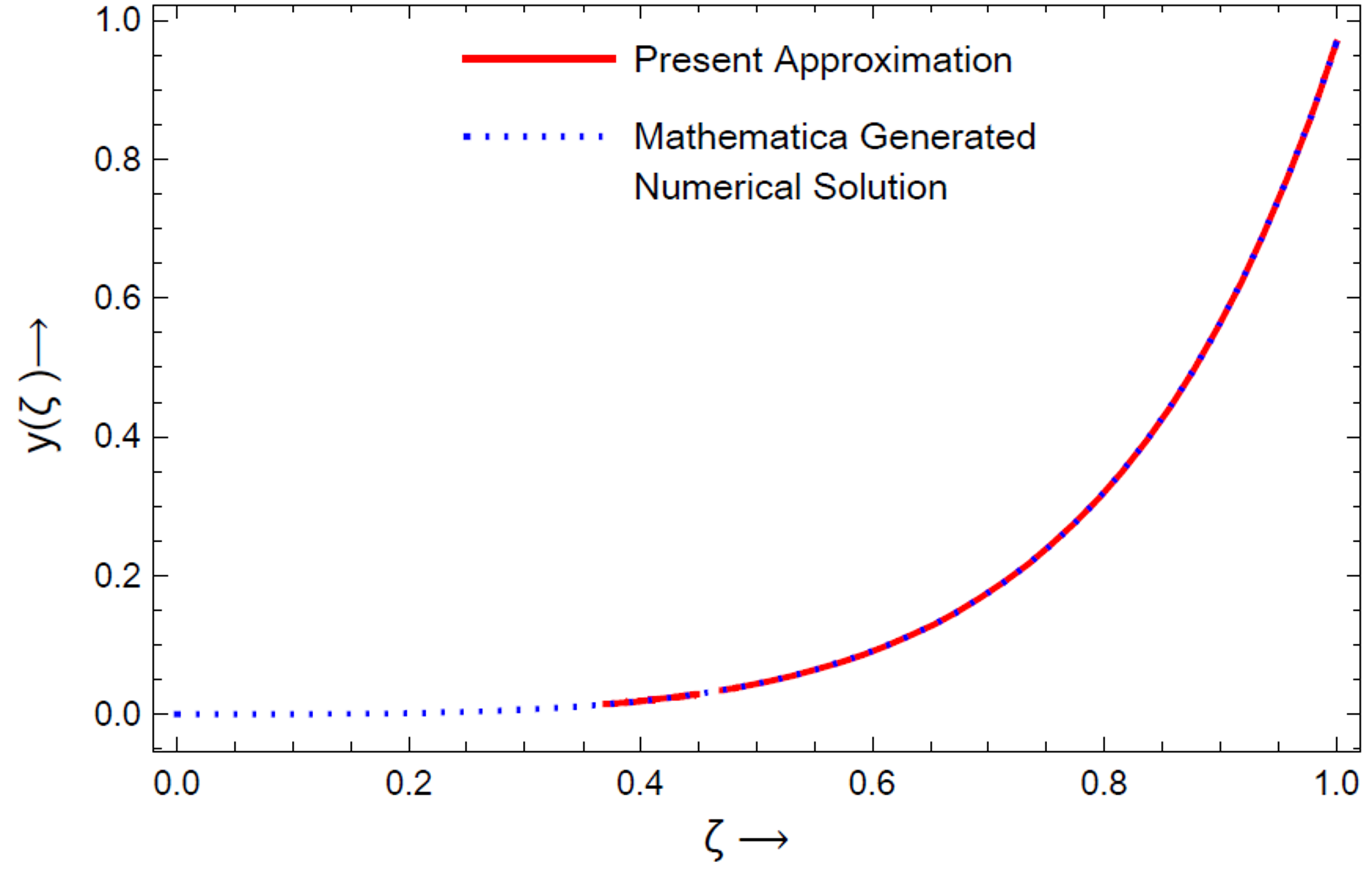
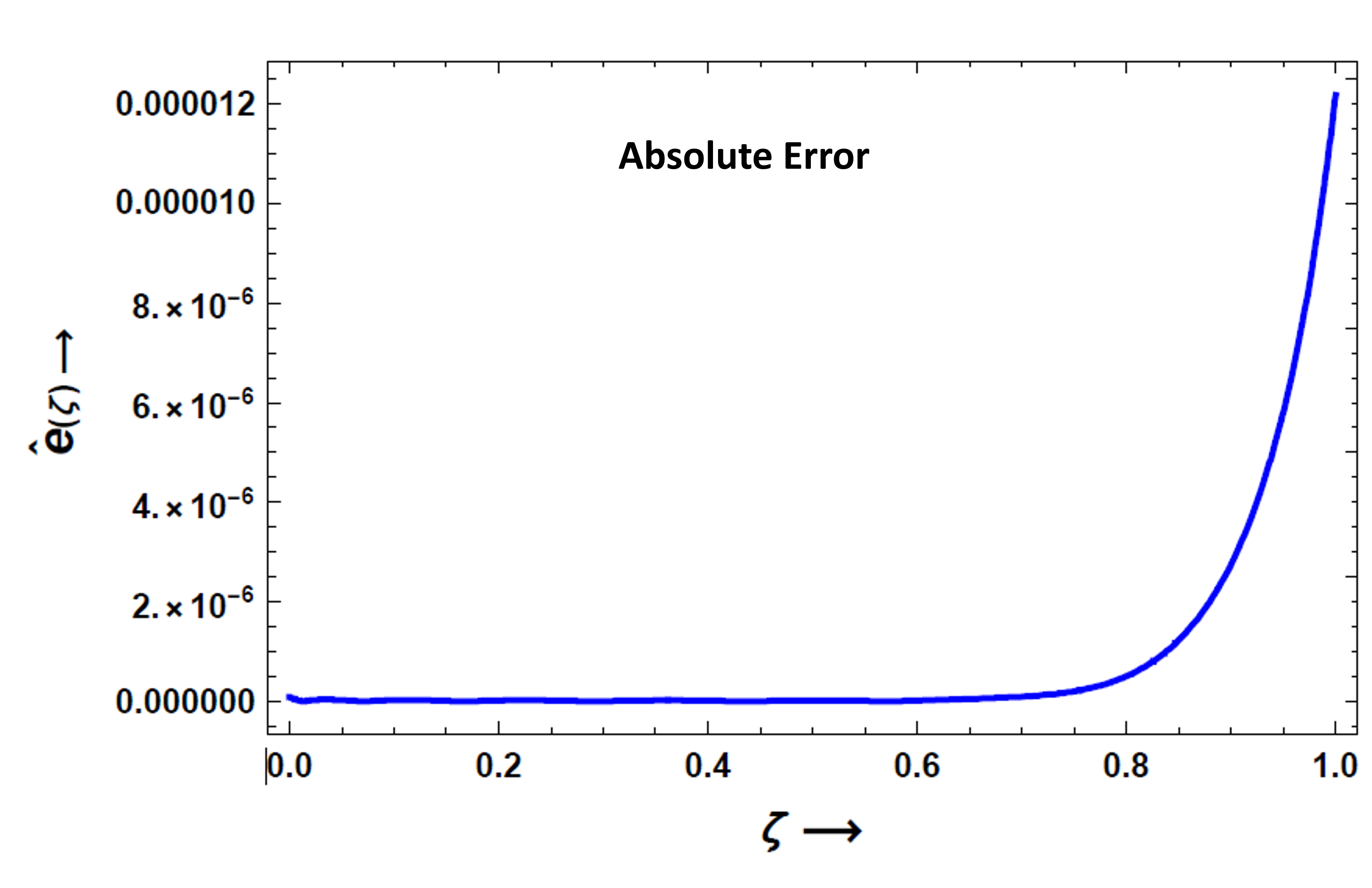
(a)                                                             (b)

Figure 2: (a) Comparison of present approximation and $Mathematica$ generated numerical solutions to example 2. (b) Absolute error between present approximation and $Mathematica$ generated numerical solutions to example 2.

Example 3:

Let us take the IVP

$$\frac{d^{2}y}{dx^{2}}+\tan(x)\frac{dy}{dx}+2\cos^{2}(x)y=2\cos^{4}(x);\hskip 10.00002pty(0)=\left(\frac{dy}{dx}\right)_{x=0}=0$$ (30)

The exact solution of this IVP is $y(x)=2-2\cos(\sqrt{2}\sin^{2}x)-\sin x$.

Using the method discussed in $section$ 6.2, coefficient vector $C^{T}$ and approximate solution $y(x)$ of example (30) is obtained for $n=6$ as:

$$C^{T}=\left(0.78730,0.62821,0.10352,-0.02660,0.00101,0.00136,0.00011\right)$$ (31)

$$y(x)\approx-0.00025+0.00718x+2.94625x^{2}+0.16696x^{3}$$

$$-1.57951x^{4}+0.17065x^{5}+0.33315x^{6}$$ (32)

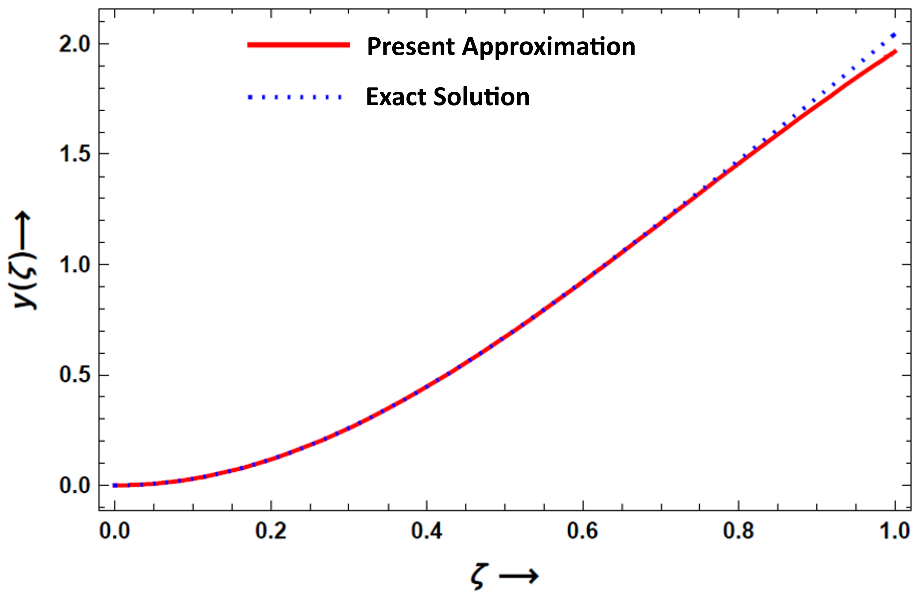
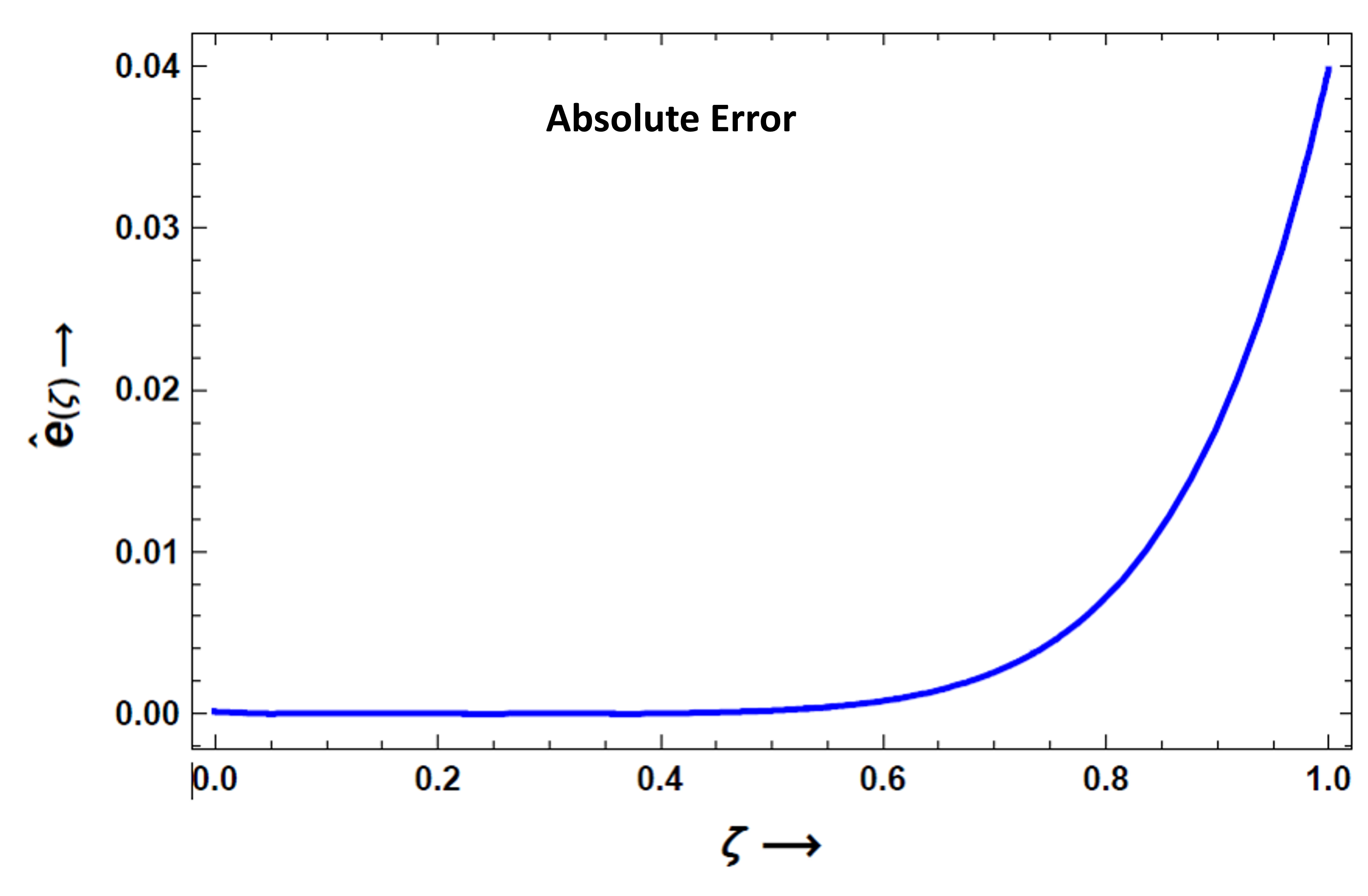
(a)                                                             (b)

Figure 3: (a) Comparison of exact solution and present approximation to example 3. (b) Absolute error between exact solution and present approximation to example 3.

8 Conclusion

In this work, a new method was presented and demonstrated to find fast and approximate solution of linear initial value problems with help of orthogonal Bernoulli polynomials. The method includes derivation of a set of $n$ orthonormal polynomials derived from Bernoulli polynomials up to degree $n$, and an operational matrix. The present method converts a given initial value problem into a system of algebraic equations with unknown coefficients, which are easily obtained with the help of operational matrix, and finally an approximate solution is obtained in form of a polynomial of degree $n$. The method has been demonstrated with three examples. The main features of this method can be summarized as:

• the method is programmable.

• solutiion is obtained in form of a polynomial of degree $n$ which can be easily used for various applications.

• error can be minimized up to required accuracy because error decreases quickly with increase of $n$-the degree of Bernoulli polynomials.

• error is negligible for simple IVPs with constant coefficients.

Appendix A

First ten orthonormal polynomials derived with Bernoulli polynomials are:

$${\phi_{0\,}}(\zeta)=1$$ (33)

$${\phi_{1}}(\zeta)=\sqrt{3}(-1+2\zeta)$$ (34)

$$\phi_{2}\left(x\right)=\sqrt{5}\left(1-6x+6x^{2}\right)$$ (35)

$$\phi_{3}(\zeta)=\sqrt{7}(-1+12\zeta-30\zeta^{2}+20\zeta^{3})$$ (36)

$$\phi_{4}(\zeta)=3(1-20\zeta+90\zeta^{2}-140\zeta^{3}+70\zeta^{4})$$ (37)

$$\phi_{5}(\zeta)=\sqrt{11}(-1+30\zeta-210\zeta^{2}+560\zeta^{3}-630\zeta^{4}+252{\zeta 5}^{)}$$ (38)

$${\phi_{6}}(\zeta)=\sqrt{13}\left(\begin{array}[]{l}1-42\zeta+420{\zeta^{2}}-1680{\zeta^{3}}\\ +3150{\zeta^{4}}-2772\zeta{}^{5}+924{\zeta^{6}}\end{array}\right)$$ (39)

$${\phi_{7}}\left(x\right)=\sqrt{15}\left(\begin{array}[]{l}-1+56x-756{x^{2}}+4200{x^{3}}\\ -11550{x^{4}}+16632{x^{5}}-12012{x^{6}}+3432{x^{7}}\end{array}\right)$$ (40)

$${\phi_{8}}\left(x\right)=\sqrt{17}\left(\begin{array}[]{l}-1+72x-1260{x^{2}}+9240{x^{3}}-34650{x^{4}}\\ +72072{x^{5}}-84084{x^{6}}+51480{x^{7}}-12870{x^{8}}\end{array}\right)$$ (41)

$${\phi_{9}}\left(x\right)=\sqrt{19}\left(\begin{array}[]{l}-1+90x-1980{x^{2}}+18480{x^{3}}-90090{x^{4}}+252252{x^{5}}\\ -420420{x^{6}}+411840{x^{7}}-218790{x^{8}}+48620{x^{9}}\end{array}\right)$$ (42)

References

- Pandey et al. [2016] R. K. Pandey, S. Sharma, K. Kumar, Collocation method for Generalized Abel’s integral equations, Journal of Computational and Applied Mathematics 302 (2016) 118–128.
- Atkinson [1997] K. E. Atkinson, The Numerical Solution of Integral Equations of the Second Kind (Cambridge Monographs on Applied and Computational Mathematics), Cambridge University Press, Cambridge, 1997.
- Samadyar and Mirzaee [2019] N. Samadyar, F. Mirzaee, Numerical scheme for solving singular fractional partial integro-differential equation via orthonormal Bernoulli polynomials, International Journal of Numerical Modelling: Electronic Networks, Devices and Fields 32 (2019).
- Bhrawy et al. [2012] A. H. Bhrawy, E. Tohidi, F. Soleymani, A new Bernoulli matrix method for solving high-order linear and nonlinear Fredholm integro-differential equations with piecewise intervals, Applied Mathematics and Computation 219 (2012) 482–497.
- Xu [2007] L. Xu, Variational iteration method for solving integral equations, Computers and Mathematics with Applications 54 (2007) 1071–1078.
- Pandey et al. [2009] R. K. Pandey, O. P. Singh, V. K. Singh, Efficient algorithms to solve singular integral equations of Abel type, Computers and Mathematics with Applications 57 (2009) 664–676.
- Cheon [2003] G. S. Cheon, A note on the Bernoulli and Euler polynomials, Applied Mathematics Letters 16 (2003) 365–368.
- Maleknejad et al. [2007] K. Maleknejad, S. Sohrabi, Y. Rostami, Numerical solution of nonlinear Volterra integral equations of the second kind by using Chebyshev polynomials, Applied Mathematics and Computation 188 (2007) 123–128.
- Nemati [2015] S. Nemati, Numerical solution of Volterra-Fredholm integral equations using Legendre collocation method, Journal of Computational and Applied Mathematics (2015).
- Rahman et al. [2012] M. A. Rahman, M. S. Islam, M. M. Alam, Numerical Solutions of Volterra Integral Equations Using Laguerre Polynomials, Journal of Scientific Research 4 (2012) 357–364.
- Yousefi [2006] S. A. Yousefi, Numerical solution of Abel’s integral equation by using Legendre wavelets, Applied Mathematics and Computation 175 (2006) 575–580.
- Sahu and Mallick [2019] P. K. Sahu, B. Mallick, Approximate Solution of Fractional Order Lane–Emden Type Differential Equation by Orthonormal Bernoulli’s Polynomials, International Journal of Applied and Computational Mathematics 5 (2019).
- Shiralashetti and Kumbinarasaiah [2018] S. C. Shiralashetti, S. Kumbinarasaiah, Hermite wavelets operational matrix of integration for the numerical solution of nonlinear singular initial value problems, Alexandria Engineering Journal 57 (2018) 2591–2600.
- Shiralashetti and Kumbinarasaiah [2019] S. C. Shiralashetti, S. Kumbinarasaiah, New generalized operational matrix of integration to solve nonlinear singular boundary value problems using Hermite wavelets, Arab Journal of Basic and Applied Sciences 26 (2019) 385–396.
- Abd-Elhameed et al. [2013] W. M. Abd-Elhameed, E. H. Doha, Y. H. Youssri, New spectral second kind Chebyshev wavelets algorithm for solving linear and nonlinear second-order differential equations involving singular and Bratu type equations, Abstract and Applied Analysis 26 (2013) 1–9.
- Iqbal et al. [2013] J. Iqbal, R. Abass, P. Kumar, Solution of linear and nonlinear singular boundary value problems using Legendre wavelet method, Italian Journal of Pure and Applied Mathematics-N 40 (2013) 311–328.
- Kumar and Singh [2009] M. Kumar, N. Singh, A collection of computational techniques for solving singular boundary-value problems, Advances in Engineering Software 40 (2009) 288–297.
- Kurt and Simsek [2011] B. Kurt, Y. Simsek, Notes on generalization of the Bernoulli type polynomials, Applied Mathematics and Computation 218 (2011) 906–911.
- Natalini and Bernardini [2003] P. Natalini, A. Bernardini, A generalization of the Bernoulli polynomials, Journal of Applied Mathematics 3 (2003) 155–163.
- Tohidi et al. [2013] E. Tohidi, A. H. Bhrawy, K. Erfani, A collocation method based on Bernoulli operational matrix for numerical solution of generalized pantograph equation, Applied Mathematical Modelling 37 (2013) 4283–4294.
- Tohidi and Kiliçman [2013] E. Tohidi, A. Kiliçman, A collocation method based on the bernoulli operational matrix for solving nonlinear BVPs which arise from the problems in calculus of variation, Mathematical Problems in Engineering 2013 (2013) 1–9.
- Mohsenyzadeh [2016] M. Mohsenyzadeh, Bernoulli operational Matrix method of linear Volterra integral equations, Journal of Industrial Mathematics 8 (2016) 201–207.
- Singh et al. [2019] M. Singh, S. Singhal, N. Handa, Exact and Numerical Solution of Abel Integral Equations by Orthonormal Bernoulli Polynomials, International Journal of Applied and Computational Mathematics 153 (2019).
- Costabile and Dell’Accio [2006] F. A. Costabile, F. Dell’Accio, A new approach to Bernoulli polynomials, Rendiconti di Matematica, Serie VII 26 (2006) 1–12.
- Todorov [1984] P. G. Todorov, On the theory of the Bernoulli polynomials and numbers, Journal of Mathematical Analysis and Applications 104 (1984) 309–350.
- E. [1978] K. E., John Wiley and Sons Press, New York, USA, 1978.
- Costabile and Dell’Accio [2001] F. A. Costabile, F. Dell’Accio, Expansion over a rectangle of real functions in bernoulli polynomials and applications, BIT Numerical Mathematics 51 (2001) 451–464.
- Lu [2011] D. Q. Lu, Some properties of Bernoulli polynomials and their generalizations, Applied Mathematics Letters 24 (2011) 746–751.