A Self-Calibrating Halo-Based Galaxy Group Finder: Algorithm and Tests

Abstract

We describe an extension of the halo-based galaxy group-finding algorithm that adds freedom to the algorithm to more accurately determine which galaxies are central and which are satellites and to provide unbiased estimates of halo masses. We focus on determination of the galaxy-halo relations for star-forming and quiescent galaxies. The added freedom in the group-finding algorithm is self-calibrated using observations of color-dependent galaxy clustering, as well as measurements of the total satellite luminosity in deep imaging data around stacked samples of spectroscopic central galaxies, $L_{\rm sat}$. We test this approach on a series of mocks that vary the galaxy-halo connection, including one mock constructed from UniverseMachine results. Our self-calibrated algorithm shows marked improvement over previous methods in estimating the color-dependent satellite fraction of galaxies. It reduces the error in $\log M_{h}$ for central galaxies by over a factor of two, to $\lesssim 0.2$ dex. Through the $L_{\rm sat}$ data, it can quantify differences in the luminosity-to-halo mass relations for star-forming and quiescent galaxies, even for groups with only one spectroscopic member. Thus, whereas previous algorithms cannot constrain the scatter in $L_{\rm gal}$ at fixed $M_{h}$, the self-calibration technique can provide a robust lower limit to this scatter.

1 Introduction

Galaxy group catalogs are one of the key tools for advancing our knowledge of galaxy formation and evolution (e.g., Huchra & Geller 1982; Eke et al. 2004; Yang et al. 2005; Berlind et al. 2006; Robotham et al. 2011; Tinker et al. 2011; Gerke et al. 2012). To robustly interpret the spectrum of galaxy properties, it is critical to understand which galaxies are central in their dark matter halo, and which are satellites orbiting within the halo potential. Armed with this ability to decompose the galaxy population in the local universe into populations of central and satellite galaxies, for example, Peng et al. (2012) found that the correlations of galaxy color with environment were driven by the rising fraction of satellite galaxies in high-density regions, and that the colors of central galaxies were nearly independent of environment (see also, Blanton & Berlind 2007; Tinker et al. 2008, 2011, 2017; Wang et al. 2018).

This central-satellite decomposition afforded by group catalogs has had other notable successes in our understanding of galaxy formation. This knowledge has yielded quenching timescales of satellite galaxies (Weinmann et al. 2010; Wetzel et al. 2013a), and central galaxies (Hahn et al. 2017). Groups catalogs have provided a model-independent confirmation of the Halo Occupation Distribution description of galaxy bias (HOD; Yang et al. 2008) as well as observational constraints on the stellar-to-halo mass relation (SHMR; see the recent review of the galaxy-halo connection by Wechsler & Tinker 2018). The information they provide is one of the primary methods of investigating the galaxy-halo connection and providing tests of galaxy formation models (e.g., Henriques et al. 2017; De Lucia et al. 2019).

Although many different definitions of galaxy groups exist in the literature, the definition that best facilitates these results is that a group of galaxies is a set of galaxies that occupy a common dark matter halo. In this vein, the true purpose of a galaxy group finder is not finding groups of galaxies, but rather to find dark matter halos and identify which galaxies reside are their centers.

Despite the many successes of modern group finders, significant problems in their efficacy hinder further progress. In this paper we will address several of these issues to construct a new group finding algorithm. All group findering algorithms contain within then free parameters. Usually, these parameters are calibrated on mock galaxy distributions. However, this means that the calibration of the group finder is sensitive to the details of the mock construction and the physical realism of the mock. Our solution is to add extra freedoms to the group-finding algorithm that directly address their current limitations, and then self-calibrate these parameters through independent observations that indirectly probe the galaxy-halo connection, such as clustering and cross-correlations with deep imaging data.

1.1 Problems in Current Group Finders

Group finding algorithms typically fall into two classifications: percolation-based finders and halo-based finders. Percolation-based finders use the friends-of-friends algorithm to link together galaxies in a group. This approach was first used on spectroscopic survey data by Huchra & Geller (1982), and then further implemented on large-scale galaxy redshift surveys in 2dFGRS (Eke et al. 2004), SDSS (Berlind et al. 2006), and GAMA (Robotham et al. 2011). Halo-based algorithms, developed by Yang et al. (2005), use our theoretical knowledge of propreties and statistics of dark matter halos to infer membership probabilities of central and satellite galaxies. We focus here on improving the halo-based group finding algorithm, but we note that many of the issues we will discuss are found in percolation-based methods as well. Campbell et al. (2015) detailed many failures of both approaches, especially in the context of understanding the galaxy-halo connection for galaxy samples broken into star-forming and quiescent samples.

1. Impurities and incompleteness in satellite galaxies. Given the fact that we don’t know the true distance to galaxies in a redshift survey, it is impossible to achieve perfect purity and completeness when assessing which galaxies are satellites within a sample. These errors are magnified when separately quantifying the satellite fractions, $f_{\rm sat}$, of red and blue galaxies. Satellites have a higher quenched fraction relative to central galaxies (Scranton 2002; van den Bosch et al. 2003; Zehavi et al. 2005, 2011; Weinmann et al. 2006; Wetzel et al. 2012). This is due to a number of physical mechanisms that can heat, strip, or cut off the gas supply of the satellite galaxy, none of which are available to central galaxies that exist in field halos. Thus, when galaxies are misclassified, this leads to an underestimate of the red satellite fraction and an overestimate of the blue satellite fraction, even if the overall $f_{\rm sat}$ is accurately gauged. When trying to compare theoretical models to observed group data, one solution to this problem is to forward model the theory by constructing a mock galaxy sample and passing it through the group finder, as done in Wetzel et al. (2012, 2013b) and Calderon et al. (2018). This is a cumbersome process and it not always available if the theory is not applied to a simulation.

2. Estimating halo masses for sub-classes of central galaxies. Most current group finders of both varieties rely on the total luminosity or stellar mass within a group to estimate the halo mass. In this method, the assigned halo masses follow the rank-ordering of the group luminosities. This becomes a problem when the SHMR of one class of galaxies differs is a systematic way to that of another class of galaxies.

Due to the fact that blue galaxies increase their stellar mass over time, while red galaxies are largely stagnant after their arrival on the red sequence it is possible that red and blue subsamples have different SHMRs. Further, the compilation of recent analyses of the red and blue SHMRs in Wechsler & Tinker (2018) shows that there is no consensus in the community on this question.

The way this introduces errors into the group-finding process is as follows: The central galaxy dominates the total luminosity and stellar mass of the group for halo masses below $\sim 10^{14}$ M_⊙ (Yang et al. 2003; Tinker et al. 2005; Vale & Ostriker 2006; Sheldon et al. 2009; Leauthaud et al. 2012; Tinker et al. 2019a), even though it may have a number of satellite galaxies. Thus, in the rank-ordering of total group luminosities, groups with red and blue central galaxies of the same luminosity will be next to each other in the rank-order, and thus be assigned the same dark matter halo mass, regardless of the physical reality. As a consequence, group finders can accrue errors of the host halo masses of nearly an order of magnitude (Campbell et al. 2015).

3. No inclusion of the scatter between halos and central galaxies. The scatter in the galaxy-halo connection is generally parameterized as a lognormal scatter of $M_{\ast}$ at fixed $M_{h}$, with width $\sigma_{\log M_{\ast}}$ (or $\sigma_{\log L}$ for $\log L_{\rm gal}$; see §4.3 in Wechsler & Tinker 2018 and references therein). This approach is in reasonable agreement with the results of hydrodynamic simulations and semi-analytic galaxy formation models (Matthee et al. 2017). In the rank-ordering scheme of halo assignment, the variation of $M_{\ast,\rm cen}$ at fixed $M_{h}$ is perfectly correlated with total stellar mass in the satellite galaxies, as $M_{h}$ is set by $M_{\ast,\rm tot}$. Thus, when the number of members in a group is reasonably large, the value of $\sigma_{\log M_{\ast}}$ in the group catalog is non-zero but typically smaller than the true value (Reddick et al. 2013; Cao et al. 2019). However, when the number of members is low, such that the total group luminosity is dominated by the central galaxy, the true scatter is entirely suppressed and central galaxies with the same luminosity will be assigned the same halo mass. Thus the value of $\sigma_{\log M_{\ast}}$ in the catalog approaches zero.

1.2 Toward a group finder that solves these problem

All galaxy grop finders have free parameters. For the Yang et al. (2005) algorithm, the unknown quantity is the threshold probability above which a galaxy can be considered a satellite of a larger halo, $B_{\rm sat}$. For the percolation algorithms of Berlind et al. (2006) and Robotham et al. (2011), it is the linking lengths for projected separation and line-of-sight separation between neighboring galaxies. In these cases, these unknowns are calibrated on mock galaxy catalogs. Thus, the values that are used to analyze real data are dependent on the details of the mock construction.

Although our knowledge of the galaxy-halo connection for luminosity or stellar mass is robust, when extended to secondary galaxy properties, such as color, star formation rate, morphology, or size, many different choices can be made. For galaxy color and star-formation rate, the mechanisms that influence galaxy growth and quenching are not fully known. Whether halos play an active or passive role in these processes is a current area of debate. For example, one may construct toy models in which central galaxy quenching is only a function of halo mass, or one in which quenching of these galaxies is entirely a function of galaxy stellar mass. These models will yield different SHMRs, even if they match observed quenched fractions. Additionally, there are number of ways to parameterize the quenching of satellite galaxies as well. Thus, the calibration of group finding free parameters on mocks may influence the end results.

The alternative we explore here is to bring in external data with which to self-calibrate the group finder’s free parameters. The primary output of a group finder is the statistical relationship between halos and galaxies—the mean number of galaxies as a function of halo mass and galaxy properties. If the group finder has done its job effectively, then the halo occupation function (HOD) estimated by the finder is representative of reality. A straightforward method of testing this is to populate the halos in a simulation with the occupation function derived by the group catalog, and compare the resulting galaxy clustering to that measured in the actual data. If the occupation function is wrong–for example, it underpredicts the fraction of red galaxies that are satellites—then the clustering will be different than the observations. This approach is related to that taken by Sinha et al. (2018), in which they use a group finder to constrain the free parameters of the HOD. In our approach the HOD is non-parametric, but the free parameters are within the group finder itself.

Clustering, however, provides limited influence on the mapping between luminosity and halo mass for central galaxies in halos of $M_{h}\lesssim 10^{13}$ M_⊙. Other information is required to decide if a central galaxy lives in a halo of $M_{h}\sim 10^{11.5}$ M_⊙, or occupies a somewhat larger $10^{12}$ M_⊙ halo, neither of which are likely to have any satellite galaxies in the spectroscopic sample being analyzed.

To address this issue, we incorporate new results of the total satellite luminosity around central galaxies, $L_{\rm sat}$, from Tinker et al. (2019a) and Alpaslan & Tinker (2020). The $L_{\rm sat}$ statistic cross-correlates central galaxies with faint imaging catalogs, far fainter than the spectroscopic limit of the SDSS Main Galaxy Sample (MGS; Strauss et al. 2002). These data supplement the spectroscopic data, filling in the gaps of our ability to connect galaxies to halos. Alpaslan & Tinker (2020) demonstrated that, at fixed stellar mass, galaxy secondary properties show strong correlations with $L_{\rm sat}$, implying that dark halos influence these properties. This result agrees with recent weak lensing results of KiDS+GAMA, in which directly measured correlations between halo mass and galaxy secondary properties at fixed stellar mass (Taylor et al. 2020).

One key result of Alpaslan & Tinker (2020) is that stellar mass does not contain the most information about $L_{\rm sat}$, and, by extension, $M_{h}$. In all cases, $r$-band absolute magnitude, $M_{r}$, of the central correlated best with $L_{\rm sat}$. Combined with persistent theoretical uncertainties in estimating stellar masses (e.g., Lower et al. 2020), and the difficulty in of creating volume-limited samples that are complete in stellar mass, these results lead us to use $r$-band luminosity, $L_{\rm gal}$, as our primary quantity to map between galaxies and halos. In analogy with the SHMR, our main quantities of interest are (1) the luminosity-to-halo mass relation, LHMR, when broken into star-forming and quiscent samples, and (2), the fraction of each sample that are satellites. For brevity, we will use “blue” and “red” to refer to these types of galaxies.

In §2, we will describe the mocks that we use to test out new algorithm. In §3, we will review the current halo-based group-finding algorithm, and present our extensions to a self-calibrated model. In §4, we will show the performance of our algorithm in recovering unbiased values of the LHMRs, $f_{\rm sat}$ values, and $\sigma_{\log L}$ values. We will summarize and discuss prospects for application of this algorithm in §5. Most results here use the high resolution Bolshoi-Planck cosmological N-body simulation (Klypin et al. 2016).

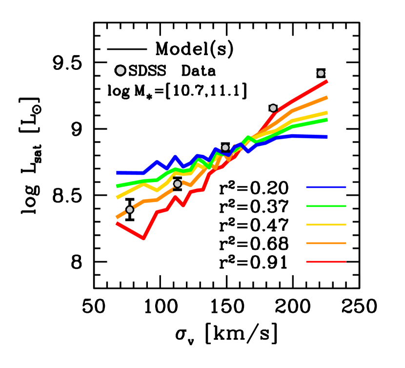
Figure 1: The correlation between $L_{\rm sat}$ and $\sigma_{v}$ for a bin in galaxy stellar mass. Points with errors are taken from Alpaslan & Tinker (2020). The multi-colored curves show theoretical models that vary the correlation between $M_{h}$ and $\sigma_{v}$ at fixed $M_{\ast}$. In order to match the observations, the correlation needs to have $r^{2}\gtrsim 0.9$, implying that $\sigma_{v}$ contains significant information about $M_{h}$. These results are the motivation behind the inclusion of the hypothetical secondary galaxy property, $\chi$, in MockB.

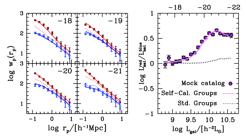
Figure 2: Observed properties of, and group finder fit to, MockA. The quartet of panels on left-hand side of the figure show the projected correlation function in bins of $r$-band magnitude, for red and blue galaxies. To conserve space, we have not shown the $-17$ bin, but the results are similar to the $-18$ bin. The measurements from the mocks are indicated by the points with error bars; red and blue colors indicate red and blue galaxies. The solid curves are the best-fit self-calibrated group catalog. The dotted curves show the prediction from the standard group finder, without self-calibration. The large panel on the right-hand side shows the $L_{\rm sat}$ ratio between red and blue galaxies at fixed $L_{\rm gal}$. Points and curves are the same as the clustering panel.

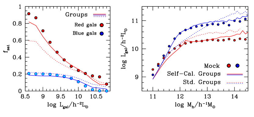
Figure 3: Left-Hand Panel: Satellite fraction, $f_{\rm sat}$, as a function of $L_{\rm gal}$, for red and blue galaxies. Colored circles show values from MockA. Dotted curves show the predictions from the standard group finder, which significantly underpredicts $f_{\rm sat}$ for red galaxies. This is consistent with the clustering of red galaxies predicted by the standard finder in Figure 2. The solid curves show the predictions from the self-calibrated group finder. Right-Hand Panel: The galaxy-halo connection for red and blue galaxies. Filled circles show the values from MockA. Solid curves show the predictions from the self-calibrated group finder. As with $f_{\rm sat}$, we stress that this is a prediction of the model. The prediction from the standard group finder, shown with the dotted curves, cannot distinguish the halos of red and blue central galaxies for $L_{\rm gal}\lesssim 10^{10.4}$ $h^{-2}{\rm L}_{\odot}$.

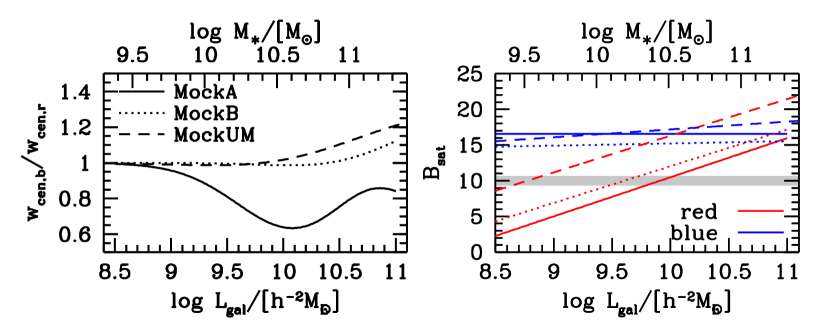
Figure 4: Left Panel: Relative weights assigned to blue and red central galaxies in the best-fit model for the three mocks. These weights are used to determine the weighted total luminosity of the group, ${L}_{\rm tot}$. The total luminosity is used in the rank-ordering of groups to assign halo mass via abundance matching via Eq. (14). The lower $x$-axis shows the luminosity of central galaxies in MockA and MockB, while the upper $x$-axis shows the stellar mass scale for MockUM. Right panel: The best-fit model for the satellite threshold values for all three mocks. Line types, and $x$-axes are the same as the key in the left panel. The standard value of $B_{\rm sat}=10$ is shown with the gray line.

2 Mock Construction

To test whether our self-calibration can work in myriad galaxy-halo connections for red and blue subsamples of galaxies, we have compiled a set of three mocks with different properties. In addition to two mock we constructed, we have also applied our algorithm to public catalogs from UniverseMachine (Behroozi et al. 2019). We use more than one mock because we want to test different LHMRs, different satellite abundances, and different input physics.

Both in-house mocks are constructed using the Bolshoi-Planck simulation (Klypin et al. 2016). We use the abundance matching technique to assign galaxy luminosity to dark matter halos. We use $M_{\rm peak}$ as the halo quantity to match to $L_{\rm gal}$. The simulation volume is 250 $h^{-1}{\rm Mpc}$ per side, yielding a volume-limited angular sample that extends to a redshift of $z=0.085$ with a footprint of 1/8^th of the full sky, or $\sim 5200$ deg². The mocks include all galaxies down to $\log L_{\rm gal}=8.66$ in the $r$-hand in solar units, equivalent to $M_{r}-5\log h=-17$. This is substantially more volume than is achievable at this magnitude limit in SDSS, but matches the depth of the ongoing Bright Galaxy Survey within the Dark Energy Spectroscopic Instrument Survey (DESI-BGS; DESI Collaboration et al. 2016), as well as the upcoming WAVES-Wide survey (Driver et al. 2016).

The mocks test a variety of situations that could plausibly arise, even though they are not necessarily representative of the actual SDSS galaxy distribution. In MockA, the galay-halo connection for red and blue galaxies are substantially different, as is the resulting measurements of $L_{\rm sat}$—at fixed halo mass, the blue galaxies are more massive than the red galaxies, while at fixed $L_{\rm gal}$, $L_{\rm sat}$ for red galaxies is higher. In MockB, the galaxy-halo connections for red and blue galaxies are different but the $L_{\rm sat}$ measurements are the same. In MockUM, the mock created from UniverseMachine, the galaxy-halo connections are the same, but the $L_{\rm sat}$ measurements are different.

The mock data on which our tests of the group finder are based—namely, the projected correlation function and the color-dependent $L_{\rm sat}$ measurements—will be presented in §4 with the results of the tests.

2.1 Total Satellite Luminosity

As discussed in the introduction, one of the main enhancements to the standard group finder in the inclusion of information from $L_{\rm sat}$ measurements. The number of subhalos within a halo, and thus the total amount of light in satellite galaxies, scales nearly linearly with the host halo mass. At low halo masses, where the average number of spectroscopic galaxies within a group is expected to be $<2$, $L_{\rm sat}$ brings extra constraining power on the halos of these galaxies.

The procedure for measuring $L_{\rm sat}$ is detailed and tested in Tinker et al. (2019a). Central galaxies from the spectroscopic MGS sample are cross-correlated with galaxies within the deep imaging of the DESI Legacy Imaging Survey (DLIS; Dey et al. 2019). The DLIS data is $\sim 6$ magnitudes fainter in the $r$-band than the MGS sample limit, making the imaging data capable of detecting satellite galaxies around the faintest of MGS central galaxies.

Without redshift information for the DLIS galaxies, satellites cannot be found in individual halos. Rather, $L_{\rm sat}$ is measured for stacked samples of central galaxies by subtracting the estimated background number of imaging galaxies projected along the line of sight. To impose minimal priors on the measurement, $L_{\rm sat}$ is evaluated in a fixed comoving aperture around each central galaxy of 50 $h^{-1}{\rm kpc}$.

Alpaslan & Tinker (2020) used these measurements to quantify the correlation between $L_{\rm sat}$ and secondary galaxy properties—i.e., size, velocity dispersion, color, morphology, etc—at fixed galaxy stellar mass. If these parameters correlated only with $M_{\ast}$ and not with the host dark matter halo, then no correlation would exist with $L_{\rm sat}$, but correlations were found with nearly all galaxy properties. An example of these results is shown in Figure 1, which we discuss further in §2.3. One of the key results is that star-forming and quiescent central galaxies had different $L_{\rm sat}$ values at fixed $M_{\ast}$. These measurements were consistent with the lensing measurements of Mandelbaum et al. (2016), in which red galaxies occupied higher mass halos than blue galaxies of the same $M_{\ast}$. The $L_{\rm sat}$ results indicated that this bimodality, which is highly significant in the weak lensing for galaxies with $M_{\ast}\gtrsim 10^{10.5}$ M_⊙, shrinks for less massive galaxies, such that faint red and blue galaxies have the same $L_{\rm sat}$ values.

These data will be critical in the self-calibration of the halo-based group finder. We note that, in order to make these $L_{\rm sat}$ measurements, a group catalog is first required in order to create a sample of central galaxies. For the purposes of these mock tests, we will use the true centrals for the $L_{\rm sat}$ mock data. When implementing on survey data, the process will have multiple iterations: the first iteration will use the previous group finder, and the second using the central galaxies from the first implementation of the self-calibrated group finder.

2.2 Mock A

To assign luminosity to the halos and subhalos in MockA, we use the Blanton et al. (2005) luminosity function. The Blanton measurement is corrected for incompleteness of low-luminosity galaxies caused by their low surface brightness, which is critical for estimating $L_{\rm sat}$ robustly. The completeness corrections increase the amplitude of the luminosity function by a factor of 3 at r-band magnitudes of $M_{r}-5\log h\sim-15$. We use a scatter in $\log L_{\rm gal}$ at fixed $M_{\rm peak}$, $\sigma_{\log L}$, of 0.2 dex.

Galaxies are assigned to be red and blue based on their luminosity and whether they are central or satellite. We set the probability that a given central galaxy is quenched to be

$$P_{q}(L_{\rm gal}|{\rm cen})=0.5\left[1+{\rm erf}\left(\frac{\log L_{\rm gal}-9.9}{0.7}\right)\right]$$ (1)

where $q$ indicates “quenched” and erf is the error function. This fitting function is calibrated to match the quenched fraction of centrals from the Tinker et al. (2011) catalog. The probability that a satellite galaxy is quenched is

$$P_{q}(L_{\rm gal}|{\rm sat})=0.4\left[1+{\rm erf}\left(\frac{\log L_{\rm gal}-9.9}{0.7}\right)\right]+0.2.$$ (2)

This function, also comparable to current group catalog results, sets a minimum quenched fraction of 20% and ensures that the quenched fraction of satellites is always higher than the quenched fraction of centrals at all luminosities.

At this stage of construction, the LHRMs are the same for central galaxies regardless of whether they are red or blue. As a simulacrum of the Mandelbaum et al. (2016) and Alpaslan & Tinker (2020) observations, we increase the luminosities of the blue galaxies by a luminosity-dependent factor,

$$\Delta\log L_{\rm gal}=0.5\left[1+{\rm erf}\left(\frac{\log L_{\rm gal}-10.0}{0.7}\right)\right].$$ (3)

Eq. (3) only makes bright blue galaxies brighter, but leaves faint blue galaxies unchanged. From the point of view of halo occupation, this makes blue galaxies brighter than red galaxies in massive halos, while preserving the $L_{\rm sat}$ observations that blue rand red galaxies have the same luminosities in lower-mass halos. Implementing Eq. (3) on the mock alters the overall luminosity function and quenched fractions to some degree, but these modifications do not subvert the physical realism of the mock—the quenched fraction still monotonically increases with $L_{\rm gal}$, and the quenched fraction of satellites is always higher than that of centrals. The final galaxy-halo relations and $f_{\rm sat}$ values for this mock will be presented in §4.1 and Figure 3, when we show the group finder predictions for these quantities.

Galaxy clustering in the mock is measured for red and blue subsamples in bins of $\log L_{\rm gal}$. To follow the convention of Zehavi et al. (2011) and other SDSS analyses, we use bins of $r$-band magnitude, with lower limits being $M_{r}-5\log h=[-17,-18,-19,-20,-21]$, with each bin being one magnitude wide. To estimate errors for the $w_{p}(r_{p})$ measurements, we use the jackknife method, dividing the plane of the sky into 25 roughly equal areas.

Even though the volume-limited mocks are constructed with $M_{r}-5\log h<-17$, the abundance matching calculation extends down to $M_{r}-5\log h<-14$, which is the magnitude limit of the $L_{\rm sat}$ data. Each galaxy in the mock-spectroscopic sample is also assigned a value of $L_{\rm sat}$, using the same aperture size as in the SDSS data. Because $L_{\rm sat}$ requires subhalos to be well-resolved at low masses, artificial disruption of substructure is a concern. In tests with smaller-volume, higher resolution simulations, we find a non-zero but small difference in $L_{\rm sat}$ for halos less massive than $\sim 10^{12}$ M_⊙ (Tinker et al. 2019b), but in the group-finding process we do not attempt to fit the absolute values of $L_{\rm sat}$—rather, we fit the relative values of $L_{\rm sat}$ for red and blue galaxies at fixed $L_{\rm gal}$, $L_{\rm sat}^{\rm red}/L_{\rm sat}^{\rm blue}$. Using relative values will ameliorate many possible systematics that may come into play; theoretical systematics such as numerical resolution or artificial disruption of satellites (e.g., van den Bosch et al. 2018) should cancel, and observational systematics such as miscalibration between the SDSS and DLIS photometry, or uncertainties in the background subtraction to make the $L_{\rm sat}$ measurements, will be attenuated as well.

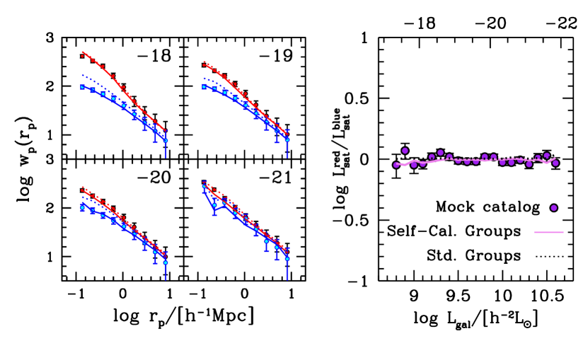
Figure 5: Observed properties of, and group finder fit to, MockB. This figure is analogous to Figure 2. The quartet of panels on left-hand side of the figure show the projected correlation function in bins of $r$-band magnitude, for red and blue galaxies. The measurements from the mocks are indicated by the points with error bars; red and blue colors indicate red and blue galaxies. The solid curves are the self-calibrated group catalog result. The dotted curves show the prediction from the standard group finder, without self-calibration. The large panel on the right-hand side shows the $L_{\rm sat}$ ratio between red and blue galaxies at fixed $L_{\rm gal}$. Points and curves are the same as the clustering panel. Because MockB is constructed to have no difference in the observed $L_{\rm sat}$ values between blue and red galaxies, the group finder fit and the prediction of standard group finder are nearly identical, and both are consistent with the mock data.

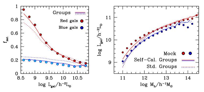
Figure 6: Predicted quantities for MockB. Left-Hand Panel: Satellite fraction, $f_{\rm sat}$, as a function of $L_{\rm gal}$, for red and blue galaxies. Colored circles show values from MockB. Dotted curves show the predictions from the old group finder, which significantly underpredicts $f_{\rm sat}$ for red galaxies. The solid curves show the predictions from the self-calibrated group finder. Right-Hand Panel: The LHMR for red and blue central galaxies. Filled circles show the values from MockB. Solid curves show the predictions from the self-calibrated group finder. The inclusion of the $\chi$-$L_{\rm sat}$ data, which we present in 7, give the algorithm the constraining power to differentiate the LHMRs of red and blue galaxies. Dotted curves show the predictions of the standard group finder, which lie directly on top of each other.

2.3 MockB

MockB is constructed under the same framework as MockA, but with many substantive changes in order to test different aspects of the group finder. First, we use the Sersic-profile $r$-band luminosity function of Bernardi et al. (2013), rather than the Blanton et al. (2005) luminosity function. The Bernardi luminosity function is consistent with Blanton at the knee of the luminosity function, but yields a much higher abundance of luminous galaxies. Thus the Bernardi LF yields a significantly different LHMR at the massive end. The fit provided in Bernardi is not valid at lower luminosities, thus we re-fit the Blanton two-Schechter functional form to match the Blanton results at $M_{r}-5\log h>-18$ and match the Bernardi measurements and brighter magnitudes.

We incorporate a halo mass-dependent $\sigma_{\log L}$. In massive halos, $M_{h}\gtrsim 10^{13}$ $h^{-1}{\rm M}_{\odot}$, we set $\sigma_{\log L}=0.2$ dex, in agreement with observations (Wechsler & Tinker 2018). Below this mass, $\sigma_{\log L}$ rises monotonically with decreasing $\log M_{h}$, to $\sigma_{\log L}=0.35$ at $M_{h}=10^{11.0}$ $h^{-1}{\rm M}_{\odot}$. This rise in scatter is seen multiple hydrodynamic simulations and measured observationally by Cao et al. (2019). Using lensing results to put a lower bound on the scatter at $M_{h}\approx 10^{12}$ $h^{-1}{\rm M}_{\odot}$, Taylor et al. (2020) also find that the scatter of $M_{\ast}$ at fixed $M_{h}$ is significantly higher than measurements at the group and cluster scale. More than just incorporating these new observations, it is of interest to determine if the self-calibrating group finder can recover a mass-variable scatter.

The quenched fractions of central and satellite galaxies follow Eqs. (1) and (2), without any shifting of the luminosities for blue or red central galaxies. Thus, when binned by stellar mass, the LHMRs of the two galaxy subsamples are the same. However, the situation when binned by halo mass is quite different. At fixed $M_{h}$, there is a distribution of $L_{\rm gal}$. But the Eq. (1) depends on $L_{\rm gal}$ only, thus quenched galaxies at fixed $M_{h}$ are more likely to be brighter than average. Thus, when plotted as a function of $M_{h}$, the LHMRs for red galaxies is shifted above that for the blue sample.

As we will demonstrate, the standard group finder does not have the constraining power to determine that the galaxy-halo connections are different for red and blue galaxies in MockB. Indeed, using clustering information and the relative $L_{\rm sat}$ values of of blue and red galaxies does not provide sufficient constraining power. The last observable included in the mocks, which we only incorporate in MockB, provides this information.

This observable is the correlation between $L_{\rm sat}$ and a secondary galaxy property at fixed $L_{\rm gal}$ for central galaxies. Our motivation for including these data come from the results of Alpaslan & Tinker 2020, which show strong correlations of $L_{\rm sat}$ with secondary galaxy properties at fixed $M_{\ast}$. An example of this is shown in Figure 1, for stellar velocity dispersion, $\sigma_{v}$. The points with errors show the measurements for central galaxies in SDSS. The steep slope implies that $\sigma_{v}$ holds significant information about the halos around them. As a demonstration of this, the solid curves show model curves that use conditional abundance matching (Hearin & Watson (2013); Hearin et al. (2014)) to match $\sigma_{v}$ to $M_{h}$ at fixed $M_{\ast}$, after abundance matching $M_{\ast}$ onto $M_{h}$ with $\sigma_{\log M_{\ast}}=0.2$. Different curves show how different correlations between $M_{h}$ and $\sigma_{v}$ yield different slopes to the $L_{\rm sat}$-$\sigma_{v}$ relation. To reproduce the observations, the coefficient of determination, $r^{2}$, must be close to unity.

For the purposes of these tests, the galaxy property shall remain hypothetical, referred to as $X$. Further, we make our mock measurements as a function of the normalized parameter $\chi\equiv(X-\bar{X})/\sigma_{X}$. As with the $L_{\rm sat}^{\rm red}/L_{\rm sat}^{\rm blue}$ measurements, we also only use $L_{\rm sat}$ relative to the mean value, i.e., $L_{\rm sat}(\chi|L_{\rm gal})/L_{\rm sat}(L_{\rm gal})$

As with the example in Figure 1, we use conditional abundance matching to incorporate a relationship between $\chi$ and $M_{h}$. The method used here is taken from Appendix A in Tinker et al. (2018a). For convenience, we assume that $\chi$ is normally distributed. In a narrow bin in $\log L_{\rm gal}$, galaxies are sorted in ascending order by $M_{h}$. We generate two Gaussian random variables with zero mean and unit variance, $G_{1}$ and $G_{2}$. $G_{1}$ is sorted in ascending order, while $G_{2}$ is left unsorted. For a given galaxy in the sorted halo list, we assign $\chi$ by the weighted sum of $G_{1}$ and $G_{2}$ such that

$$\chi=G_{1}\times\frac{r^{2}}{\mathcal{R}}+G_{2}\times\frac{(1-r^{4})^{1/2}}{\mathcal{R}},$$ (4)

where $r$ is the correlation coefficient and ${\mathcal{R}}$ is a normalization constant to preserve the unit Gaussian distribution of $\chi$. Because the scatter is lognormal in $L_{\rm gal}$, it will be approximately lognormal in $M_{h}$ at fixed $L_{\rm gal}$, thus Eq. (4) correlates $\chi$ with $\log M_{h}$. If $r=1$, then $\chi=G_{1}$ and the random variables is perfectly correlated with $\log M_{h}$. If $r=0$, then $\chi=G_{2}$ and each galaxy is assigned a $\chi$ randomly. For the mock, we measure $L_{\rm sat}^{\rm red}/L_{\rm sat}^{\rm blue}$ for five bins in $\log L_{\rm gal}$ 0.5 dex in width, with the bin centers at $\log L_{\rm gal}=[9.0,9.5,10.0,10.5,11.0]$.

Our fiducial version of MockB has $r^{2}=0.86$, which yields correlations between $\chi$ and $L_{\rm sat}$ that are consistent with that seen in Figure 1, and other properties investigated in Alpaslan & Tinker (2020). We also construct versions of MockB with $r^{2}=1$ and $r^{2}=0.71$.

2.4 Universe Machine Mock

We use the public data release of UniverseMachine DR1 for the $z=0$ output of the Bolshoi-Planck simulation. These data include halo mass, galaxy stellar mass, and star formation rate. We therefore use $M_{\ast}$ rather than $L_{\rm gal}$ as the base galaxy property to correlate with $M_{h}$. To separate galaxies in red and blue subsamples, we use the specific star formation rate, $\rm sSFR=\rm SFR/M_{\ast}$, with a break point at $\log\rm sSFR=-11$, which cleanly separates the two populations in SDSS data (Wetzel et al. 2012; Hahn et al. 2017; Tinker et al. 2018a).

The public data release doe not include luminosity information, thus we assign values of $L_{\rm sat}$ to each halo from the list of halos produced for MockA. For each UM halo, we find the 20 halos from MockB closest by their mass, and then select $L_{\rm sat}$ randomly from that list of 20. We check this measurement of $L_{\rm sat}^{\rm red}/L_{\rm sat}^{\rm blue}$ by comparing it to summing the stellar mass in satellites within the same projected separation as $L_{\rm sat}$ measurements, and find that $M_{\ast\rm sat}^{\rm red}/M_{\ast\rm sat}^{\rm blue}$ is consistent with our approach. We will quantitatively compare the two in §4.5.

From the UM DR1 data, we construct a volume-limited mock complete down to $M_{\ast}=10^{9.0}$ M_⊙. This yields a galaxy number density that is 0.77 times that of the luminosity-defined mocks. Clustering of the red and blue subsamples is measured in bins of $\log M_{\ast}$ that are 0.5 dex wide, with the lower limit of each bin being $\log M_{\ast}=[9.0,9.5,10.0,10.5,11.0]$.

MockUM differs from the luminosity-defined mocks in several important ways. First, although MockUM is built upon the Bolshoi-Planck simulation, Behroozi et al. (2019) employ ‘orphan’ satellites to track galaxies that reside in subhalos that have become numerically disrupted. Thus the overall number of satellite galaxies will be higher in MockUM, as well as their spatial distribution within their host halos. Second, UniverseMachine uses empirical forward-modeling to match observed galaxy statistics as a function of redshift, tracking individual halos as they evolve across cosmic time. Thus, galaxy quenching is not a simple function of $L_{\rm gal}$ as in MockA and MockB. Quenching probability correlates with halo properties, including mass and formation history.

As with MockA, we do not incorporate the galaxy secondary parameter, $\chi$.

3 Group Finding Methods

Here we outline both the original halo-based algorithm, then describe the extensions to this algorithm. We define halos as virialized, spherical objects such that

$$M_{\Delta}=\frac{4}{3}\pi R^{3}_{\Delta}\Delta\bar{\rho}_{m}.$$ (5)

where $\Delta$ is the mean overdensity of the halo and $\bar{\rho}_{m}$ is the mean matter density of the universe in comoving units. Thus, the comoving radius of a halo is independent of redshift at fixed mass. In this definition, $\Delta$ is a free parameter. So long as the choice is well-motivated and consistent throughout all calculations, the results and insensitive to the specific value of $\Delta$. Here we choose $\Delta=200$, thus $M_{h}=M_{200}$.

We further assume that all halos follow the universal density profile of Navarro et al. (1996) (NFW), which parameterizes the profile through a single free parameter, referred to as the scale radius of the halo, $r_{s}$;

$$\rho_{h}(r)=\frac{\rho_{0}}{(r/r_{s})(1+r/r_{s})^{2}}$$ (6)

where $\rho_{0}$ is a normalization constant determined by the mass of the halo. The concentration of a halo is the ratio of the halo radius to the scale radius, $c_{\Delta}=R_{\Delta}/r_{s}$. Concentration and mass are weakly correlated with each other, with a spread of $\sim 0.12$ dex in $\log c$ at fixed $M_{h}$ (e.g., Bullock et al. 2001). We are not able to infer concentrations of individual groups, thus we assume that all halos fall on the mean concentration-mass relation of Macciò et al. (2008).

From the virial theorem, the velocity dispersion within the dark matter within a halo is

$$\sigma_{v}^{2}=\frac{GM_{\Delta}}{2R_{\Delta}}(1+z),$$ (7)

where the factor of $(1+z)$ converts comoving radius $R_{\Delta}$ to physical units.

3.1 Basic Algorithm for the Halo-Based Group Finder

The basic algorithm employed by Tinker et al. (2011) is presented here, which follows Yang et al. (2005), with minor modifications. We expand on some of the steps in the subsequent text as necessary.

1. Inverse-abundance match to assign initial halo masses to galaxies, and label all galaxies as central.

2. Sort galaxies by halo mass in descending order.

3. In that order, for each central galaxy, determine the membership probability of neighboring (lower-luminosity) galaxies. If the probability is above a threshold value, assign that neighbor as a satellite to the central galaxy. If a central galaxy in the list has been re-classified as a satellite of a brighter galaxy, skip this step for that re-classified galaxy.

4. For each group, sum the total amount of luminosity (or stellar mass).

5. Sort the groups by total luminosity in descending order.

6. Assign halo masses to the groups by inverse-abundance matching.

7. If the value of $f_{\rm sat}$ is converged, then exit. Otherwise, sort the central galaxies by halo mass and return to step 3.

1. Abundance matching is a technique to assign galaxies to dark matter halos in simulations (Kravtsov et al. 2004; Vale & Ostriker 2006; Conroy et al. 2006; Wechsler & Tinker 2018). Here, we proceed in the opposite direction—we assign halo masses to galaxies. In this step, we use the simplest form of abundance matching, expressed as

$$\int_{L_{\rm gal}}^{\infty}\Phi(L_{\rm gal}^{\prime})\,dL_{\rm gal}^{\prime}=\int_{M_{h}}^{\infty}n(M_{h}^{\prime})\,dM_{h}^{\prime},$$ (8)

where $\Phi(L_{\rm gal})$ is the galaxy luminosity function and $n(M_{h})$ is the halo mass function. By matching the cumulative abundances of galaxies and halos, Eq. (8) states that galaxies of luminosity $L_{\rm gal}$ reside in halos of mass $M_{h}$. This implementation assumes no scatter between halo and galaxy properties, which we do not have the power (yet) to constrain. When applying Eq. (8) to all galaxies in a sample, the LHMR produced is a poor approximation of the true relation at the the luminous end, but it is accurate enough to serve as a starting point of the algorithm. It also has the benefit of taking negligible computing time, in comparison to friends-of-friends group finders or other percolation methods. At this point in the algorithm, every galaxy is classified as ‘central’ for the purposes of group-finding.

3. The probability that a neighbor galaxy is a member of a given group is separated into two components; one based on the projected separation between the neighbor and the central galaxy, and the line-of-sight separation of the neighbor and central. The critical insight of the Yang et al. (2005) algorithm is that we can bring in our prior knowledge of dark matter halos from numerical simulations to inform these choices.

We assume that satellite galaxies within a group are spatially distributed the same as the dark matter within the halo. Thus, we can use the NFW profile in Eq (6) to quantify the relative probability that a neighbor with separation $R_{p}$ is satellite within a given halo. The projected probability, $P_{\rm proj}$, is equal to the projected, normalized NFW density profile, expressed by Yang et al. (2005) as

$$P_{\rm proj}(R_{p})=2r_{s}\bar{\delta}{f(R_{p}/r_{s})}\,,$$ (9)

where $R_{p}$ is the comoving projected separation between the central galaxy and the candidate satellite galaxy,

$$f(x)=\left\{\begin{array}[]{lll}\frac{1}{x^{2}-1}\left(1-\frac{{\ln{\frac{1+\sqrt{1-x^{2}}}{x}}}}{\sqrt{1-x^{2}}}\right)&\mbox{if $x<1$}\\ \frac{1}{3}&\mbox{if $x=1$}\\ \frac{1}{x^{2}-1}\left(1-\frac{{\rm atan}\sqrt{x^{2}-1}}{\sqrt{x^{2}-1}}\right)&\mbox{if $x>1$}\end{array}\right.\,,$$ (10)

and

$$\bar{\delta}={200\over 3}{c_{200}^{3}\over{\rm ln}(1+c_{200})-c_{200}/(1+c_{200})}.$$ (11)

For an isothermal, isotropic velocity distribution of satellites, with velocity dispersion given by Eq. (7), the line-of-sight probability that a galaxy with redshift separation $\Delta z=z_{\rm cen}-z$ is

$$P_{z}(\Delta z)=\frac{c}{\sqrt{2\pi}\sigma_{v}}\exp\left[\frac{-(c\Delta z)^{2}}{2\sigma_{v}^{2}}\right],$$ (12)

where $c$ is the speed of light. For a galaxy with projected separation $R_{p}$ and line-of-sight separation $\Delta z$ from a given central galaxy, we set the probability that it is satellite as

$$P_{\rm sat}=\left[1-\left(1+P_{\rm proj}P_{z}/B_{\rm sat}\right)^{-1}\right],$$ (13)

where $B_{\rm sat}$ is a free parameter. In the Yang et al. (2005) implementation, this parameter was calibrated on mocks, with a value of $B_{\rm sat}=10$. This value was also used in the Tinker et al. (2011) implementation. If $P_{\rm sat}>0.5$ then it is classified as a satellite for that group. $P_{\rm sat}$ is not a true probability, but rather a quantity that correlates with our confidence the classification of a given galaxy. The utility of having a continuous variable for $P_{\rm sat}$ is to construct ‘pure’ samples of central galaxies, where one has higher confidence that each galaxy in the sample is indeed a true central, at the cost of some completeness of the sample.

6. Inverse-abundance matching to assign halo mass to total group luminosity requires a minor modification of Eq. (8) to

$$\int_{L_{\rm grp}}^{\infty}n(L_{\rm grp}^{\prime})\,dL_{\rm grp}^{\prime}=\int_{M_{h}}^{\infty}n(M_{h}^{\prime})\,dM_{h}^{\prime},$$ (14)

where $n(L_{\rm grp})$ is the abundance of the groups.

3.2 Extension and Self-Calibration

To construct a self-calibrated group finder, we extend the halo-based algorithm, and incorporate new data, in three key ways.

1. Allowing variability in $B_{\rm sat}$: The threshold for assigning a galaxy to be a satellite within a group is set by Eq. (13). We first break $B_{\rm sat}$ into separate values for red and blue galaxies, $B_{\rm sat,r}$ and $B_{\rm sat,b}$. Each of these thresholds is then allowed to vary as a function of galaxy luminosity:

$$B_{\rm sat,c}=\beta_{0,c}+\beta_{L,c}(\log L_{\rm gal}-9.5),$$ (15)

where the subscript $c={r,b}$ refers to the different color samples, with $r$=red and $b$=blue.

Constraining power from the data: Eq. (15) gives us four free parameters, two for red galaxies and two for blue. The data most useful for constraining these parameters are the projected correlation functions of red and blue galaxies. $w_{p}(r_{p})$. As discussed in the introduction, if the group finder has correctly assigned galaxies to halos, then the halo occupation produced by the group finder should accurately predict the clustering of galaxies. Two-point clustering, especially at scales of $r_{p}\lesssim 1$ $h^{-1}{\rm Mpc}$, is especially sensitive to the fraction of galaxies that are satellites, $f_{\rm sat}$. After fitting for $w_{p}(r_{p})$, to confirm that the group catalog is self-consistent, we check that the catalog correctly reproduces the input value of $f_{\rm sat}$ as a function of $L_{\rm gal}$ for mock red and blue galaxies.

2. Weighting the luminosity of red and blue central galaxies. To account for the fact that red and blue central galaxies may have different luminosities at fixed halo mass, we weight the central galaxy luminosity when compiling the list of total group luminosities used Eq. (14) to assign halo mass. The log of the weight factor, $w_{\rm cen}$ scales with luminosity as:

$$\log w_{\rm cen,c}=\frac{\omega_{0,c}}{2}\left[1+{\rm erf}\left(\frac{\log L_{\rm gal}-\omega_{L,c}}{\sigma_{\omega,c}}\right)\right],$$ (16)

where $c=r$ or $b$ to indicate galaxy color. The form of Eq. (16) affords maximum flexibility in the weight factors. Positive and negative values of $\omega_{0}$ will either upweight or downweight groups in the rank-ordered list. The characteristic luminosity $\omega_{L}$ allows galaxies to be unweighted at either low or high luminosities, and $\sigma_{\omega}$ allows the weights to turn on abruptly, or to extend the transition so wide that all galaxies in the sample receive equal up- or down-weight. We implement Eq. (16) separately for red and blue central galaxies, creating six free parameters. Having separate weights for the two samples increases the flexibility further, allowing the relative weights between the two to be non-monotonic. Because we are less concerned with constraining the free parameters than constraining the LHMRs, many degrees of freedom—which possibly create degeneracies in the parameter space—is not a concern.

Constraining power from the data: Most of the constraining power on $w_{\rm cen,r}$ and $w_{\rm cen,b}$ comes from measurements of the $L_{\rm sat}^{\rm red}/L_{\rm sat}^{\rm blue}$ ratio. This quantity is closely related to the ratio of host halo masses at fixed $L_{\rm gal}$. If this ratio deviates from unity, then these galaxies occupy different halos. This does not mean that the LHMRs must be different—it may be that the LHRMs are the same, but different values of $\sigma_{\log L}$ may cause differences in $M_{h}$ when binned by $L_{\rm gal}$.

Although some inference on $w_{\rm cen,r}$ and $w_{\rm cen,b}$ comes from the clustering data, the constraining power of $w_{p}(r_{p})$ for central galaxies is limited. Measurements of clustering amplitude at large scales is often used to infer halo mass, but for $M_{h}\lesssim 10^{13}$ $h^{-1}{\rm M}_{\odot}$ in the local universe, the halo bias function flattens out, thus it is difficult to infer much about central masses in the same way that clustering can constrain satellite fractions.

3. Individual weights on based on secondary galaxy properties. Figure 1, demonstrates that individual properties of galaxies contain information about their host halos at fixed $L_{\rm gal}$. Motivated by these results, we include weight factors based on the hypothetical normalized galaxy property $\chi$, such that

$$w_{\chi}=\exp(\chi/\omega_{\chi}).$$ (17)

We further separate these weight factors for red and blue galaxies, $w_{\chi,r}$ and $w_{\chi,b}$, thus creating two new free parameters, $\omega_{\chi,r}$ and $\omega_{\chi,b}$. The exponential form of Eq. (17) is motivated by the log-linear results in Figure 1. We separate red and blue galaxy samples because the correlations between galaxy properties and $L_{\rm sat}$ are usually different, and the properties themselves can vary systematically between red and blue galaxies—for example, in relation to Figure 1, at fixed $M_{\ast}$ blue galaxies have lower $\sigma_{v}$ than red galaxies. (See the extensive discussion in Alpaslan & Tinker 2020).

Constraining power from the data: These two weight factors are primarily constrained by the measurements described in MockB: $L_{\rm sat}(\chi|L_{\rm gal})/L_{\rm sat}(L_{\rm gal})$. Including the $w_{\chi}$ weights will change the scatter in the LHMR, and can thus alter predictions for the $L_{\rm sat}^{\rm red}/L_{\rm sat}^{\rm blue}$ ratio, as well as influence the large-scale galaxy bias for luminous samples of galaxies. But the influence of these data is secondary.

3.3 Group Finding and Fitting Procedure

Our self-calibrated group finder has 12 free parameters. Four govern satellite occupation, six control the relative LHRMs of red and blue central galaxies, and the last two control individual weights on red and blue central galaxies. These parameters are compiled together in Table 1. To find the optimal parameters of the group finder, we use the following data vector of observables from the mocks described in §2:

• $w_{p}(r_{p})$ for red and blue galaxies in 5 bins of magnitude. Each measurement has 9 bins in $r_{p}$, logarithmically spaced between $r_{p}=0.1$ and 10 $h^{-1}{\rm Mpc}$.

• $L_{\rm sat}^{\rm red}/L_{\rm sat}^{\rm blue}$ for central galaxies, measured in 16 bins of $\log L_{\rm gal}$. Error bars are estimated using the bootstrap resampling method.

• For MockB only: $L_{\rm sat}(\chi|L_{\rm gal})/L_{\rm sat}(L_{\rm gal})$ for central galaxies, measured in 5 bins of $\log L_{\rm gal}$. This is done separately for both red and blue galaxies.

• For the UM mock, the number of data points is the same as for MockA, but $w_{p}(r_{p})$ and $L_{\rm sat}$ quantities are binned in $\log M_{\ast}$ as opposed to luminosity.

For a given set of parameters, the group finder is run using the procedure outlined in the basic algorithm in §3.1. The only change in the basic algorithm is in the extra freedom in $B_{\rm sat}$ and the total luminosity of the group that is used to rank-order the groups in the abundance matching halo mass assignment. Under the new algorithm, the group luminosity is

$$L_{\rm grp}=L_{\rm cen}\times w_{\rm cen,c}\times w_{\chi,c}+\sum_{i=1}^{N_{\rm sat}}L_{{\rm sat},i}$$ (18)

,

where $w_{\chi}=1$ MockA and MockUM. This yields a label of ‘central’ or ‘satellite’ for each galaxy in the mock sample, as well as an estimated halo mass. From this catalog, we make predictions for all the quantities in the list above.

For $w_{p}(r_{p})$, we measure the mean halo occupation functions for red and blue galaxies in the same magnitude bins for which $w_{p}(r_{p})$ is measured. These HODs are tabulated separately for central and satellite galaxies. The halos of our N-body simulation are then populated according to these HODs, assuming a Poisson distribution for satellites and a Bernoulli distribution for centrals. For each color and bin in $M_{r}-5\log h$, we use the corrfunc code to measure the group finder’s prediction for $w_{p}(r_{p})$ (Sinha & Garrison 2020). We then calculate the $\chi^{2}$ for each $w_{p}(r_{p})$ prediction.

For $L_{\rm sat}^{\rm red}/L_{\rm sat}^{\rm blue}$, we assign a value of $L_{\rm sat}$ to each halo from a tabulated list of the mean $L_{\rm sat}$ as a function of $M_{h}$. This list is constructed from the same N-body simulation used for $w_{p}(r_{p})$ prediction. We have tested assigning each group catalog halo a value of $L_{\rm sat}$ from an individual halo in the N-body simulation, but in practice find that this only imparts noise in the prediction without changing the mean. After each halo in the catalog has been assigned $L_{\rm sat}$, we separate the red and blue central galaxies and measure $L_{\rm sat}^{\rm red}/L_{\rm sat}^{\rm blue}$ in the same manner as the mock observations.

For MockB, we use the $L_{\rm sat}$ values assigned to each halo in the group catalog to measure $L_{\rm sat}/\bar{L}_{\rm sat}$ in the same manner as in the mock observations. The total $\chi^{2}$ for the data vector is then

$$\chi^{2}_{\rm tot}=\sum_{\rm r,b}\sum_{i=1}^{N_{\rm bins}}\left[\chi^{2}_{w_{p},i}+\chi^{2}_{\chi,i}\right]+\chi^{2}_{Lr/Lb}$$ (19)

where $N_{\rm bins}=5$ is the number of luminosity bins, noting once again that $\chi^{2}_{\chi}$ is only included for MockB. We use Powell’s method (e.g., Press et al. 1992) to minimize $\chi^{2}_{\rm tot}$, yielding the best-fit galaxy group catalog for each mock.

Although the primary results of this paper are based on the Bolshoi-Planck simulation, we have found that the results of the group finder are insensitive to which simulation is used to make the predictions of the group catalog. We have performed tests using different simulations to make the group-finder predictions, including the original Bolshoi simulation, which has different initial conditions and different cosmology, and the SMDPL which has a larger volume as well as higher mass resolution.

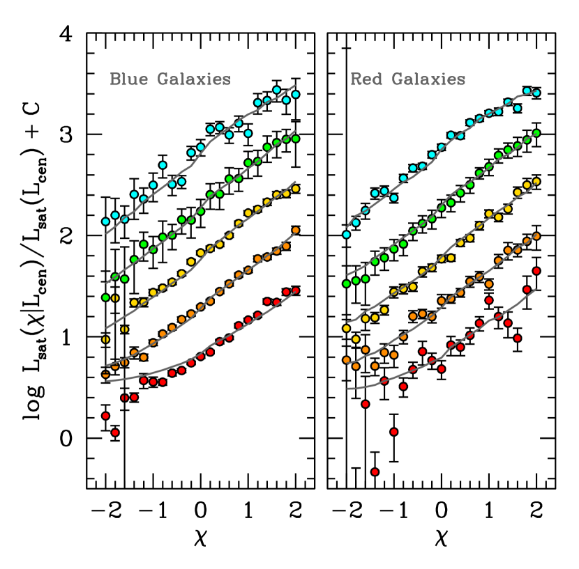
Figure 7: The correlation between $L_{\rm sat}$ and a hypothetical normalized central galaxy property, $\chi$, in MockB. This specific realization of MockB has a coefficient of determination, $r^{2}$, of 0.87. Each set of points shows the mock measurements in bins of $L_{\rm gal}$. The $L_{\rm sat}$ values are normalized by the mean value of $L_{\rm sat}$ in the bin in $L_{\rm gal}$. To differentiate the points within each panel, we have added an offset to each $L_{\rm gal}$ bin. Error bars are estimated using jackknife resampling. In each panel, the solid curves show the results of the best-fit self-calibrated group finder.

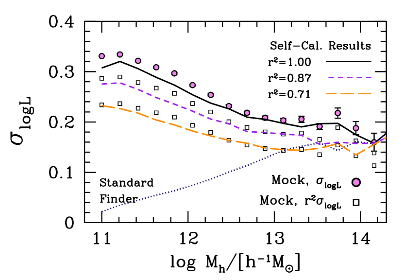
Figure 8: The scatter of $\log L_{\rm gal}$ at fixed $M_{h}$, $\sigma_{\log L}$. The filled circles show $\sigma_{\log L}$ in MockB. The dotted curve shows the results of the standard group finder, which is not able to differentiate halos of central galaxies with the same luminosity when only the central is the only galaxy in the group. The other curves show the results of the self-calibrated group finder applied to different versions of MockB where the value of $r^{2}$ is varied. The open squares show the scatter in MockB multiplied by $r^{2}$.

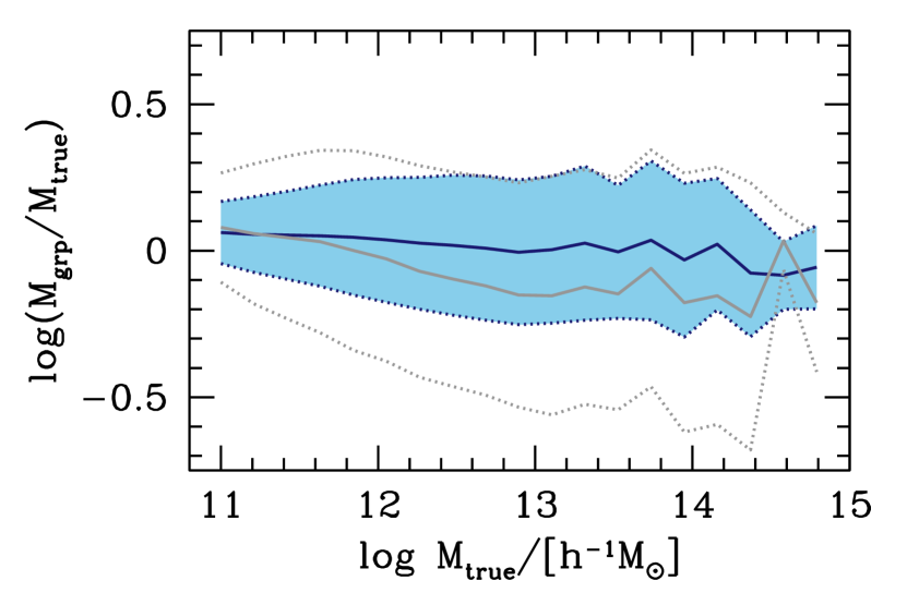
Figure 9: Errors in halo mass from the analysis of MockB with $r^{2}=0.87$. The blue cuves show the results from the self-calibrated group finder, where the solid curve is the mean halo mass and the dotted curves indicate the inner-68% range of values. The results from the standard group finder are shown with the gray curves, indicating that the self-calibrated algorithm yields roughly a factor of two improvement in the accuracy of $\log M_{h}$. The inclusion of the $\chi$-$L_{\rm sat}$ data from Figure 7 provides the information that improves these constraints. Increasing $r^{2}$ shrinks the shaded region. Increasing $\sigma_{\log L}$ in the mock will increase the errors for both algorithms.

Table 1: Parameters of the Self-Calibrated Group Finder

Parameter	Purpose	Equation	MockA	MockB	MockUM
$\beta_{0,b}$	blue satellite threshold	Eq. (15)—$B_{\rm sat,b}$	16.56	15.07	15.81
$\beta_{L,b}$	blue satellite threshold	Eq. (15)—$B_{\rm sat,b}$	-0.01	0.31	1.36
$\beta_{0,b}$	red satellite threshold	Eq. (15)—$B_{\rm sat,r}$	7.74	9.46	9.86
$\beta_{L,b}$	red satellite threshold	Eq. (15)—$B_{\rm sat,r}$	5.58	5.14	6.36
$\omega_{0,b}$	weight blue centrals	Eq. (16)—$w_{\rm cen,b}$	-1.13	0.76	-1.11
$\omega_{L,b}$	weight blue centrals	Eq. (16)—$w_{\rm cen,b}$	10.39	10.94	10.62
$\sigma_{\omega,b}$	weight blue centrals	Eq. (16)—$w_{\rm cen,b}$	0.93	0.78	0.73
$\omega_{0,r}$	weight red centrals	Eq. (16)—$w_{\rm cen,r}$	-0.93	0.66	-0.78
$\omega_{L,r}$	weight red centrals	Eq. (16)—$w_{\rm cen,r}$	10.44	10.92	10.46
$\sigma_{\omega,r}$	weight red centrals	Eq. (16)—$w_{\rm cen,r}$	0.55	0.84	0.56
$\omega_{\chi,b}$	$\chi$-property weight	Eq. (17)—$w_{\chi,b}$	—	1.60	—
$\omega_{\chi,r}$	$\chi$-property weight	Eq. (17)—$w_{\chi,r}$	—	1.52	—

Note. — MockB is the only mock that includes the measurements of the correlation between $L_{\rm sat}$ and the normalized galaxy property, $\chi$. Thus the values of $\omega_{\chi,r}$ and $\omega_{\chi,b}$ are only listed for the fiducial version of this mock, which has $r^{2}=0.87$.

4 Mock Results and Results on Mocks

Before discussing the performance of the self-calibrated group finder, we first describe the general characteristics of MockA and the performance of the previous halo based group finder, outlined in §3.1. We refer to the previous algorithm as the ‘standard group finder.’ We focus on the observable quantities—$w_{p}(r_{p})$ and $L_{\rm sat}$—and the predicted quantities of $f_{\rm sat}$ and the LHMR.

The left-hand side of Figure 2 is a quartet of panels plotting the color-dependent clustering in bins of magnitude. Consistent with SDSS results (Zehavi et al. 2011), the red galaxies in the mock are significantly more clustered than the blue galaxies. This is due to the higher $f_{\rm sat}$ for red galaxies relative to blue galaxies. On the right-hand side of the Figure is the ratio of the $L_{\rm sat}$ values for red and blue central galaxies. As discussed in §2, the blue galaxies in MockA are brighter than the red galaxies at fixed halo mass. Thus, when binning by the $L_{\rm gal}$, the halo masses—and therefore the $L_{\rm sat}$ values—for the red galaxies are higher.

Figure 2 highlights several of the issues of the standard group finder discussed in the introduction. The dotted curves in all panels show the results of applying the standard group finder to MockA, with $B_{\rm sat}=10$. For blue galaxies, the halo occupation inferred by the standard finder yields clustering that is in good agreement with the clustering of the mock catalog, but the halo occupation of the red galaxies underpredicts the clustering by a significant amount. In the right-hand panel, the standard group finder yields a $L_{\rm sat}^{\rm red}/L_{\rm sat}^{\rm blue}$ ratio that is nearly unity across the full range of central galaxy luminosity, even though the blue galaxies in the mock reside in more massive galaxies. In the mock, the red central galaxies will have more spectroscopic satellite galaxies than the blue central galaxies at fixed $L_{\rm gal}$, but this effect by itself is not enough to yield the proper halo masses.

The color-dependent satellite fractions of the mock, $f_{\rm sat}$, are shown in the left-hand side of Figure 3. For blue galaxies, $f_{\rm sat}$ is largely constant with $L_{\rm gal}$ until galaxies get brighter than the knee in the luminosity function $(L_{\rm gal}\sim 10^{10.04}$ $h^{-2}{\rm L}_{\odot}$, according to the Blanton et al. 2003 results). $f_{\rm sat}$ for red galaxies monotonically increases with decreasing $L_{\rm gal}$, reaching $\sim 90\%$ at $L_{\rm gal}\approx 10^{8.7}$ $h^{-2}{\rm L}_{\odot}$. These results are consistent with the HOD fitting of SDSS clustering in Zehavi et al. (2011). Here we see the reason that the standard group finder woefully underpredicts the small-scale clustering of red galaxies: the predicted $f_{\rm sat}$ is much lower than the mock value, never getting higher than $\sim 60\%$. The $f_{\rm sat}$ for blue galaxies is slightly higher than the mock value—the overall $f_{\rm sat}$ (not plotted) is in good agreement with the standard mock, but this agreement is due to a cancellation of errors by overpredicting the number of blue satellites and underpredicting the number of red satellites. At low luminosities most galaxies are blue, so the discrepancy is much larger for the red sample.

The right-hand side of Figure 3 shows the LHMRs for red and blue galaxies. The mean $L_{\rm gal}$ for blue and red central galaxies diverge at $M_{h}\gtrsim 10^{11.5}$ $h^{-1}{\rm M}_{\odot}$, but because the central galaxy dominates the total luminosity in the group, the standard finder has no way of determining this. Thus, the standard finder’s LHMRs for red and blue central galaxies only separate at much higher $M_{h}$, once the number of satellite galaxies in the halos dominates the total luminosity in the halo. These problems are ameliorated substantially in the self-calibrated algorithm, the results of which we show presently.

4.1 MockA

The solid curves in both sides of Figure 2 show a markedly improved comparison to the mock data relative to the results from the standard group finder. In the left-hand side, showing the color-dependent clustering, the improved fit by the self-calibrated group finder is due mainly to the extra freedom in the thresholds that determine inclusion as a satellite in a larger group. The best-fit parameters, listed in Table 1, indicate that $B_{\rm sat,r}$ is much lower than the fiducial value of 10, with a significant positive slope with $\log L_{\rm gal}$. $B_{\rm sat,b}$ is still constant with luminosity, but the best-fit value is 16.6. Both of these adjustments yield a good fit to the clustering, as well as an improved comparison to the satellite fractions in the left-hand side of Figure 3.

The self-calibrated finder also yields a good fit to the $L_{\rm sat}$ data in the right-hand panel of Figure 2. This is due to the weights, $w_{\rm cen,r}$, and $w_{\rm cen,b}$, that are applied to the luminosities of the central galaxies when rank-ordering the groups for halo mass assignment. Figure 4 shows the ratio of $w_{\rm cen,b}/w_{\rm cen,r}$ for the best-fit model. The difference at the low-mass end, $M_{h}\lesssim 10^{11.5}$, is due mainly to how the samples are binned; the mock sample has a hard cutoff at $L_{\rm gal}=10^{8.6}$ $h^{-2}{\rm L}_{\odot}$, while the group catalog yields a cutoff at fixed halo mass. Thus, even though the intrinsic relations may be equivalent in the mock and the catalog, the binned quantities can diverge when the bins encompass the limits of the sample.

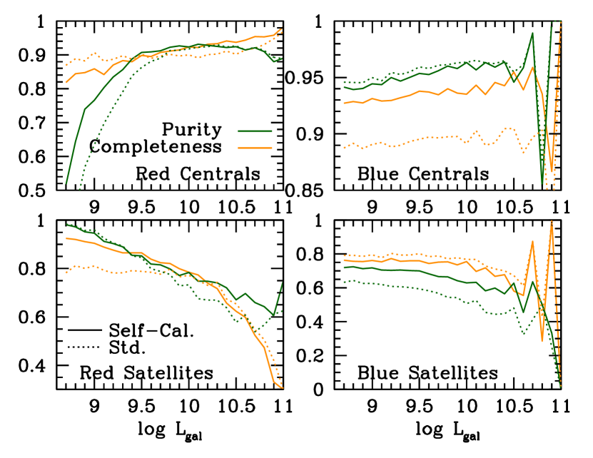
Figure 10: Purity and completeness for group finders applied to MockB. Solid curves indicate results results from the self-calibrated algorithm while dotted curves show the results from the standard group finder. Results are broken down into four galaxy classifications: red centrals, blue centrals, red satellites, and blue satellites. Completeness is defined as the fraction of galaxies in a given classification in the mock that have the same classification in the group catalog. Purity is the fraction of galaxies in a given classification in the group catalog that have the same classification in the mock. Note the change in $y$-scale in each of the panels.

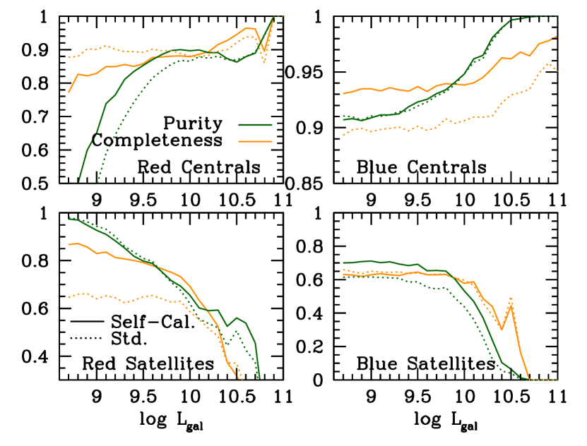
Figure 11: Purity and completeness for group finders applied to MockA. All curves and definitions are the same as Figure 10.

]

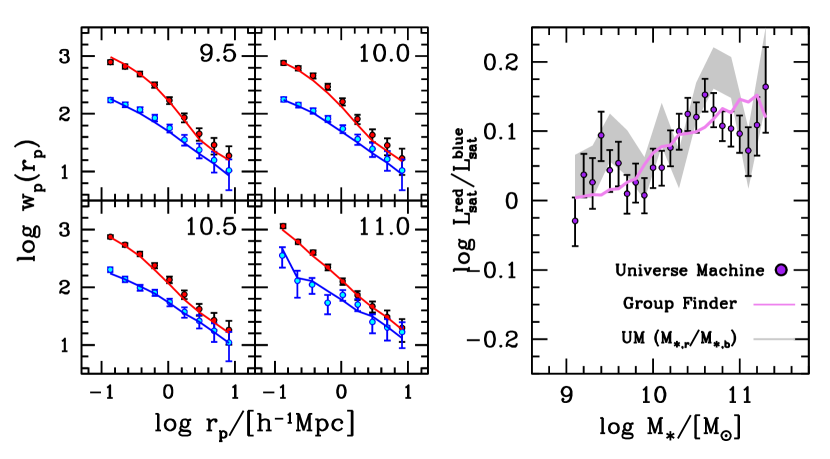
Figure 12: Observed properties of, and group finder fit to, MockUM. The quartet of panels on left-hand side of the figure show the projected correlation function in bins of $\log M_{\ast}$, for red and blue galaxies. The measurements from the mocks are indicated by the points with error bars; red and blue colors indicate red and blue galaxies. The solid curves are the best-fit group catalog result. The large panel on the right-hand side shows the $L_{\rm sat}$ ratio between red and blue galaxies at fixed $L_{\rm gal}$. Points and curves are the same as the clustering panel.

4.2 MockB: $f_{\rm sat}$ and LHMR

The clustering and $L_{\rm sat}$ observables for MockB are shown in Figure 5. While the clustering is very similar to that of MockA, the $L_{\rm sat}$ values are quite different, with the $L_{\rm sat}$ ratio being equal to unity across the full range of central galaxy luminosity. The satellite fractions and LHMRs for red and blue galaxies in the mock are shown in Figure 6. The satellite fractions are similar to MockA, but the LHMR for red galaxies is slightly higher than that for blue galaxies at all halo masses. The reason for the difference is discussed in §2.3, due to the criteria by which galaxies are assigned their colors.

The results of the standard group finder are shown in each panel in both figures with the dotted lines. In contrast to MockA, the clustering of red galaxies is well-fit by the standard finder. However, now the clustering of blue galaxies is significantly higher than the mock observables. The source of the discrepancy with the clustering of blue galaxies is found in the left-hand side of Figure 6; the satellite fraction of blue galaxies is $\sim 25\%$ higher than the mock value of $0.20$. The dramatic difference in the clustering highlights the sensitivity of $w_{p}(r_{p})$ to $f_{\rm sat}$.

Because the mock is constructed to have $L_{\rm sat}$ values the same for red and blue central galaxies, the standard finder yields a good fit to the $L_{\rm sat}^{\rm red}/L_{\rm sat}^{\rm blue}$ observable, shown in Figure 5. In the right-hand side of Figure 6, the standard finder yields LHMRs for red and blue galaxies that are virtually identical. The shape of both LHMRs is somewhat steeper than the mock values as well. This is due to the increasing fraction of red galaxies with $L_{\rm gal}$; at low $L_{\rm gal}$, most galaxies are blue and thus both LHMRs track that of the blue LHMR of the mock. At higher $L_{\rm gal}$, most galaxies are red, thus the dotted lines track the red LHMR.

In both figures, the result of the self-calibrated galaxy group finder are shown with the solid lines. MockB has the addition of the $\chi$-parameter, and its correlation with $L_{\rm sat}$. Figure 7 shows the correlation between $\chi$ and $L_{\rm sat}$, in bins of $L_{\rm gal}$, broken into red and blue galaxies. In each bin of $L_{\rm gal}$, the results are normalized by the mean $L_{\rm sat}$ within the bin. For plotting purposes, we offset each $L_{\rm gal}$ bin by a constant that increases monotonically with bin luminosity. The curves show the best-fit model from the self-calibrated group finder. Recall that the coefficient of determination is $r^{2}=0.87$ for this model, which yields correlations of $L_{\rm sat}$ with $\chi$ that are consistent with the Alpaslan & Tinker (2020) results. The best-fit weight parameters are $\omega_{\chi,r}=1.5$ and $\omega_{\chi,b}=1.6$. These values vary inversely with $r^{2}$, as larger values of $\omega_{\chi}$ reduce the $w_{\chi}$ weights in Eq. (17). For the versions of MockB with $r^{2}=1.0$ and $0.71$, the values of $\omega_{\chi}$ are 1.3 and 1.9, respectively, for both red and blue galaxies.

Figure 6 compares the self-calibrated group finder’s prediction for the LHMRs to the actual values in the mock. The prediction correctly separates the LHMRs between the two, with the red galaxies being $\sim 0.2$ dex higher in luminosity at fixed $M_{h}$. It is the inclusion of the $\chi$-$L_{\rm sat}$ data that allows the self-calibrated group finder to correctly determine that the LHMRs for red and blue galaxies are distinct. The $L_{\rm sat}^{\rm red}/L_{\rm sat}^{\rm blue}$ data are equal to unity, and are well-fit by the standard group finder. But the $\chi$-$L_{\rm sat}$ data provides information on the scatter of $L_{\rm gal}$ at fixed $M_{h}$, which drives the difference in the LHMRs. We discuss scatter in more detail presently.

4.3 MockB: Scatter and Mass Errors

The addition of the $\chi$ parameter in the model fitting allows us to differentiate the halo masses of galaxies in halos that have no spectroscopic satellites. Thus, this additional freedom makes the new group finder able to estimate the scatter of $\log L_{\rm gal}$ at fixed $M_{h}$, $\sigma_{\log L}$. Figure 8 shows the true scatter in MockB, as well as the results of various implementations of the self-calibrating group finder. As described in §2, the input scatter is variable, being consistent with observational constraints of $\sigma_{\log L}\sim 0.2$ at high masses, and increasing to $\sim 0.35$ at low $M_{h}$. The scatter estimated by the standard group finder is shown with the dotted black curve. At $M_{h}\gtrsim 10^{13}$ $h^{-1}{\rm M}_{\odot}$, it estimates a value of $\sigma_{\log L}$ $\sim 30\%$ below the true value, consistent with results from Reddick et al. (2013) and Cao et al. (2019). However, as also shown in these works, the scatter in the standard group catalog approaches zero as $M_{h}$ approaches the minimum halo mass in the catalog.

The results of the self-calibrating group finder are shown with the other curves in Figure 8. Here, we show the results for three different versions of MockB, with values of $r^{2}=0.71$, 0.875 and 1.0. The true $\sigma_{\log L}$—and all other properties of the mock—do not change; only the value of $r^{2}$ and thus the slope of the correlation between $\chi$ and $L_{\rm sat}$ (e.g., Figure 1. When $r^{2}=1.0$, i.e., the normalized galaxy property $\chi$ correlates perfectly with the halo mass, the new finder recovers the true scatter of the mock. When $r^{2}$ is below unity, the variance in $\chi$ no longer encodes all the information about the variance in $M_{h}$, thus the new finder’s estimate of $\sigma_{\log L}$ is biased low relative to the true value. Figure 8 shows that that scatter inferred by the group finder is equivalent to $r^{2}\times\sigma_{\log L}$.

The inclusion of the $\chi$-$L_{\rm sat}$ data increases the finder’s ability to accurately estimate halo masses themselves. Figure 9 shows the ratio of the halo mass assigned by the group finder to the true halo mass within the mock, $\log(M_{\rm grp}/M_{\rm true})$, as a function of $M_{\rm true}$. At $10^{13}$ $h^{-1}{\rm M}_{\odot}$, the standard deviation is $\sim 0.2$ dex, which is roughly a factor of two improvement over the standard group finder. The self-calibrated algorithm also yields unbiased halo masses, correcting the small bias of $\sim 0.1-0.15$ dex in the standard finder.

4.4 Purity and Completeness

Figure 10 compares the purity and completeness in the self-calibrated group catalog to the standard group catalog when applied to MockB. We calculate these quantities for four classifications of galaxies: red central galaxies, blue central galaxies, red satellite galaxies, and blue satellite galaxies. We define completeness as the fraction of galaxies in original mock that have the same classification in the group catalog. We define purity as the fraction of galaxies in the group catalog that have the same classification in the original mock.

Although the self-calibrated group finder shows higher purity and completeness relative to the standard finder, we not that this is not always the case. The standard finder outperforms by $\sim 5\%$ the self-calibrated algorithm in the completeness of low-luminosity red central galaxies. This is a result of the enhanced purity of red centrals in the self-calibrated catalog, which yields an improvement of $\sim 15\%$ in that quantity. There is a competition between purity and completeness, especially when the subsample in question—red centrals—is the smallest category.

The self-calibrated group finder yields most notable improvements in the completeness of blue centrals, the completeness of red satellites and low luminosities and the purity within the same classification at high luminosities, and the purity of blue satellites at all masses. The competition between purity and completeness causes the self-calibrated algorithm to do slightly worse than the standard approach in the purity of blue centrals and the completeness of blue satellites. But the improvements gained by self-calibration are significantly larger.

To see how the use of the $\chi$-$L_{\rm sat}$ data in MockB impacts the purity and completeness, we also show the same statistics, but for MockA, in Figure 11. The comparisons between the standard and self-calibrated algorithms are analogous to those in Figure 10. Differences in the overall curves at high luminosities, $L_{\rm gal}\gtrsim 10^{10}$ $h^{-2}{\rm L}_{\odot}$ are driven by the use of the Blanton luminosity function, which falls off much more rapidly than the Bernardi luminosity function.

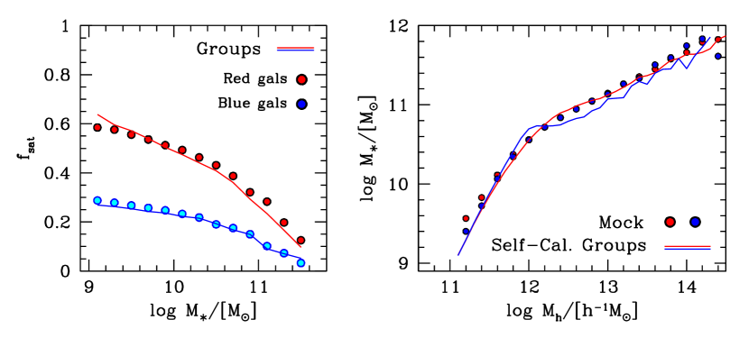
Figure 13: Left-Hand Panel: Satellite fraction, $f_{\rm sat}$, as a function of $M_{\ast}$, for red and blue galaxies. Colored circles show values from MockUM. The solid curves show the predictions from the self-calibrated group finder. Right-Hand Panel: The SHMRs for red and blue galaxies. Filled circles show the values from MockUM. Solid curves show the predictions from the self-calibrated group finder.

4.5 UniverseMachine

Figures 12 and 13 show the mock values from the UniverseMachine mock and the best-fit model of the self-calibrating group finder. Here, stellar mass is the quantity by which we rank-order the groups. Although the red galaxy clustering is enhanced relative to the that of the blue galaxies, like the luminosity mocks and the SDSS MGS results, $f_{\rm sat}$ for red galaxies is significantly lower than those results, while $f_{\rm sat}$ for blue galaxies is $\sim 50\%$ higher—$f_{\rm sat}=0.3$ versus 0.2. The $L_{\rm sat}^{\rm red}/L_{\rm sat}^{\rm blue}$ ratio is slightly above unity, even though the SHMRs are approximately the same. The self-calibrated group finder produces good fits to both the clustering and the $L_{\rm sat}$ ratio, which yield accurate predictions of the satellite fraction and the SHMRs for the red and blue samples. The paucity of blue central galaxies in halos above $10^{12}$ $h^{-1}{\rm M}_{\odot}$ creates noise in the blue SHMR, but the self-calibrated finder predicts that the SHMRs of the color samples are roughly equal. The SHMR for blue galaxies is somewhat underpredicted, by $\sim 0.15$ dex.

The gray shaded region shows the ratio total satellite stellar mass, rather than our fiducial approach of satellite luminosity. This is to compare our method of assigning $L_{\rm sat}$ to UM halos—which is based on $M_{h}$ only—to the intrinsic values from the UM model. As discussed previously, galaxy quenching in UM depends on multiple factors, including halo formation history, which may correlate with the number of subhalos in a given halo. However, the $L_{\rm sat}$ ratio is consistent with the $M_{\ast,\rm sat}$ ratio, implying that the empirically-driven quenching processes are not significantly impacting the observables used in the self-calibration process.

5 Caveats and Future Work

Although the self-calibrated group finding algorithm developed here presents a potential solution to some of the problems inherent to group finders, some issues remain.

Group Centering: This standard halo-based algorithm constructs a group catalog where the central galaxy is always the brightest in the halo. This is also the choice in the percolation-based algorithm of Berlind et al. (2006). The algorithm of Eke et al. (2004) and Robotham et al. (2011) chooses the brighter of the two galaxies closest to the luminosity-weighted group center. For the vast number of halos, these are reasonable assumptions. However, given the scatter between $M_{h}$ and $L_{\rm gal}$, combined with the fact that $d\log L_{\rm gal}/d\log M_{h}<1$ at high halo masses, some fraction of halos will contain a piece of substructure that contains a galaxy brighter than the central galaxy. This has been detected, statistically, in observational data, by Skibba et al. (2011).

The self-calibrated algorithm we describe in the proceeding section also makes this assumption. Improving on this assumption is a topic of current research, which we leave to a future paper. We can estimate the degree of the problem through our abundance matching calculations, but the results depends on the assumptions made. Assuming the Blanton et al. (2005) luminosity function and $\sigma_{\log L}=0.2$, for halos with $M_{h}\geq 10^{13}$ $h^{-1}{\rm M}_{\odot}$, a subhalo is brighter than the central 26% of the time. However, expressed as the fraction of groups with centrals brighter than $M_{r}-5\log h<-21$—the luminosity scale at which the mean halo mass is also $\sim 10^{13}$ M_⊙, this occurs only 3.3% of the time. These assumptions maximize this frequency. Lange et al. (2019) constrain $\sigma_{\log L}$ using satellite kinematics (as opposed to other recent works that measure $\sigma_{\log M_{\ast}}$) at $M_{h}\gtrsim 10^{13}$ to be $\sim 0.15$, and to be a decreasing function with increasing $M_{h}$. Using this value, and the Bernardi et al. (2013) luminosity function, these values become 5.0% for halos and 1.5% for groups.

As can be seen from our mock results, misidentification of the central galaxy has limited impact on our results. The LHMR and SHMR values recovered are unbiased relative to the input values in the mocks. The most direct consequence is in estimating $f_{\rm sat}$ for bright galaxies—if a the brightest galaxy in a group is always considered the central, this artificially suppresses $f_{\rm sat}$ at the bright end (Reddick et al. 2013). This effect can be seen in our results (e.g., Figures 3, 6, and 13).

Galaxy Assembly Bias: An inherent assumption in all halo-based group-finders—indeed, in any group finder that uses $L_{\rm grp}$ to estimate $M_{h}$—is that the amount of light in satellite galaxies is a function of the halo mass only. For dark matter halos, we know that the number of halos depends on the formation history of the halo as well (Zentner et al. 2005; Gao & White 2007; Croft et al. 2012; Mao et al. 2018). At fixed $M_{h}$, older halos have less substructure. This is one of the many manifestations of halo assembly bias (e.g., Wechsler & Tinker 2018). How much this propagates into the population of satellite galaxies—e.g., whether there is significant galaxy assembly bias—is not clear. Alpaslan & Tinker (2020) find a small but non-zero trend of $L_{\rm sat}$ decreasing with large-scale density. The trend goes in the direction expected—older halos live in higher-density environments, thus the expectation is that $L_{\rm sat}$ should decrease with density. However, the amplitude of the change in $L_{\rm sat}$ is only $\sim 2\%$ at the highest and lowest values of density measured. If galaxy assembly bias exists, it is not a strong effect on the total luminosity in satellite galaxies. Predictions of $L_{\rm sat}$ from the IllustrisTNG hydrodynamic galaxy formation simulation (Pillepich et al. 2018) are in agreement with the observational results, showing little to no correlation of $L_{\rm sat}$ with large-scale density (Cao et. al., in prepration).

An additional concern is the use of $L_{\rm sat}$ data with secondary galaxy properties. If a galaxy property correlates with halo formation history at fixed $M_{\ast}$, then the correlation of that property with $L_{\rm gal}$ would trace galaxy assembly bias, as opposed to constraining $M_{h}$. The bimodal distribution of galaxy colors and star-formation activity has been a focus of observational studies of assembly bias, with most studies finding that the data are inconsistent with strong a correlation between whether a galaxy is on the red sequence and halo formation history, and weaker correlations are difficult to detect observationally (Tinker et al. 2008, 2017, 2018b; Zu & Mandelbaum 2016, 2018; Calderon et al. 2018). The lensing results of Mandelbaum et al. (2016), demonstrating that red central galaxies live in more massive halos than blue centrals at fixed $M_{\ast}$, are in agreement with the $L_{\rm sat}$ results for red and blue galaxy samples, implying that $L_{\rm sat}$ is probing $M_{h}$ for this galaxy property.

For the hypothetical galaxy property, $\chi$, an observational test proposed by Tinker et al. (2019a) is whether the value of $\chi$ correlates with large-scale density. Alpaslan & Tinker (2020) find that the properties of red central galaxies are all consistent with no correlation with large-scale density, but for blue galaxies there are non-zero correlations for stellar velocity dispersion, galaxy size, and Sersic index. Calderon et al. (2018) also find a possible assembly bias signal for Sersic index as well. This limits the choices available for $\chi$ on real data, but candidates remain, including galaxy concentration and surface density.

Future Work: The self-calibrated group finder is ready to be run on SDSS MGS data. All clustering and $L_{\rm sat}$ data are already in place and results will come in a companion paper to this one.

DESI-BGS has begun taking data, and by the end of the first year of observations (out of five total) will have four times as many redshift as the MGS. The longer redshift baseline afforded by the BGS, which will target galaxies $\sim 2$ magnitudes deeper than the SDSS limit, will open the door to investigating evolution of the galaxy-halo connection with a single galaxy sample.

Future development of the self-calibration algorithm will also help utilize the constraining power offered by ongoing and upcoming surveys. Specifically in regards to the possibility of galaxy assembly bias, rather than selecting galaxy properties that appear to lack any detectable correlation with secondary halo properties, future implementations may rather lean in to these observed signals, with the goal of estimating not just the halo masses of galaxy groups, but other halo properties as well. New data will be required to constrain these new freedoms in the model, but upcoming data is well-positioned to provide robust measurements of statistics sensitive to assembly bias, including density correlations (Abbas & Sheth 2006; Tinker et al. 2018a), marked correlation functions (Skibba et al. 2006; Zu & Mandelbaum 2018; Calderon et al. 2018), void statistics (Tinker et al. 2008; Walsh & Tinker 2019), and the cosmic web (Tojeiro et al. 2017).

References

- Abbas & Sheth (2006) Abbas, U., & Sheth, R. K. 2006, MNRAS, 372, 1749, doi: 10.1111/j.1365-2966.2006.10987.x
- Alpaslan & Tinker (2020) Alpaslan, M., & Tinker, J. L. 2020, MNRAS, doi: 10.1093/mnras/staa1844
- Behroozi et al. (2019) Behroozi, P., Wechsler, R. H., Hearin, A. P., & Conroy, C. 2019, MNRAS, 488, 3143, doi: 10.1093/mnras/stz1182
- Berlind et al. (2006) Berlind, A. A., Frieman, J., Weinberg, D. H., et al. 2006, ApJS, 167, 1, doi: 10.1086/508170
- Bernardi et al. (2013) Bernardi, M., Meert, A., Sheth, R. K., et al. 2013, ArXiv e-prints. https://arxiv.org/abs/1304.7778
- Blanton & Berlind (2007) Blanton, M. R., & Berlind, A. A. 2007, ApJ, 664, 791, doi: 10.1086/512478
- Blanton et al. (2005) Blanton, M. R., Lupton, R. H., Schlegel, D. J., et al. 2005, ApJ, 631, 208, doi: 10.1086/431416
- Blanton et al. (2003) Blanton, M. R., Hogg, D. W., Bahcall, N. A., et al. 2003, ApJ, 592, 819, doi: 10.1086/375776
- Bullock et al. (2001) Bullock, J. S., Kolatt, T. S., Sigad, Y., et al. 2001, MNRAS, 321, 559
- Calderon et al. (2018) Calderon, V. F., Berlind, A. A., & Sinha, M. 2018, MNRAS, 480, 2031, doi: 10.1093/mnras/sty2000
- Campbell et al. (2015) Campbell, D., van den Bosch, F. C., Hearin, A., et al. 2015, MNRAS, 452, 444, doi: 10.1093/mnras/stv1091
- Cao et al. (2019) Cao, J.-z., Tinker, J. L., Mao, Y.-Y., & Wechsler, R. H. 2019, arXiv:1910.03605. https://arxiv.org/abs/1910.03605
- Conroy et al. (2006) Conroy, C., Wechsler, R. H., & Kravtsov, A. V. 2006, ApJ, 647, 201, doi: 10.1086/503602
- Croft et al. (2012) Croft, R. A. C., Matteo, T. D., Khandai, N., et al. 2012, MNRAS, 425, 2766, doi: 10.1111/j.1365-2966.2012.21438.x
- De Lucia et al. (2019) De Lucia, G., Hirschmann, M., & Fontanot, F. 2019, MNRAS, 482, 5041, doi: 10.1093/mnras/sty3059
- DESI Collaboration et al. (2016) DESI Collaboration, Aghamousa, A., Aguilar, J., et al. 2016, ArXiv e-prints. https://arxiv.org/abs/1611.00036
- Dey et al. (2019) Dey, A., Schlegel, D. J., Lang, D., et al. 2019, AJ, 157, 168, doi: 10.3847/1538-3881/ab089d
- Driver et al. (2016) Driver, S. P., Davies, L. J., Meyer, M., et al. 2016, The Universe of Digital Sky Surveys, 42, 205, doi: 10.1007/978-3-319-19330-4_32
- Eke et al. (2004) Eke, V. R., Baugh, C. M., Cole, S., et al. 2004, MNRAS, 348, 866, doi: 10.1111/j.1365-2966.2004.07408.x
- Gao & White (2007) Gao, L., & White, S. D. M. 2007, MNRAS, 377, L5, doi: 10.1111/j.1745-3933.2007.00292.x
- Gerke et al. (2012) Gerke, B. F., Newman, J. A., Davis, M., et al. 2012, ApJ, 751, 50, doi: 10.1088/0004-637X/751/1/50
- Hahn et al. (2017) Hahn, C., Tinker, J. L., & Wetzel, A. 2017, ApJ, 841, 6, doi: 10.3847/1538-4357/aa6d6b
- Hearin & Watson (2013) Hearin, A. P., & Watson, D. F. 2013, MNRAS, 435, 1313, doi: 10.1093/mnras/stt1374
- Hearin et al. (2014) Hearin, A. P., Watson, D. F., Becker, M. R., et al. 2014, MNRAS, 444, 729, doi: 10.1093/mnras/stu1443
- Henriques et al. (2017) Henriques, B. M. B., White, S. D. M., Thomas, P. A., et al. 2017, MNRAS, 469, 2626, doi: 10.1093/mnras/stx1010
- Huchra & Geller (1982) Huchra, J. P., & Geller, M. J. 1982, ApJ, 257, 423, doi: 10.1086/160000
- Klypin et al. (2016) Klypin, A., Yepes, G., Gottlöber, S., Prada, F., & Heß, S. 2016, MNRAS, 457, 4340, doi: 10.1093/mnras/stw248
- Kravtsov et al. (2004) Kravtsov, A. V., Berlind, A. A., Wechsler, R. H., et al. 2004, ApJ, 609, 35
- Lange et al. (2019) Lange, J. U., van den Bosch, F. C., Zentner, A. R., Wang, K., & Villarreal, A. S. 2019, MNRAS, 487, 3112, doi: 10.1093/mnras/stz1466
- Leauthaud et al. (2012) Leauthaud, A., George, M. R., Behroozi, P. S., et al. 2012, ApJ, 746, 95, doi: 10.1088/0004-637X/746/1/95
- Lower et al. (2020) Lower, S., Narayanan, D., Leja, J., et al. 2020, arXiv:2006.03599, arXiv:2006.03599. https://arxiv.org/abs/2006.03599
- Macciò et al. (2008) Macciò, A. V., Dutton, A. A., & van den Bosch, F. C. 2008, MNRAS, 391, 1940, doi: 10.1111/j.1365-2966.2008.14029.x
- Mandelbaum et al. (2016) Mandelbaum, R., Wang, W., Zu, Y., et al. 2016, MNRAS, 457, 3200, doi: 10.1093/mnras/stw188
- Mao et al. (2018) Mao, Y.-Y., Zentner, A. R., & Wechsler, R. H. 2018, MNRAS, 474, 5143, doi: 10.1093/mnras/stx3111
- Matthee et al. (2017) Matthee, J., Schaye, J., Crain, R. A., et al. 2017, MNRAS, 465, 2381, doi: 10.1093/mnras/stw2884
- Navarro et al. (1996) Navarro, J. F., Frenk, C. S., & White, S. D. M. 1996, ApJ, 462, 563. http://adsabs.harvard.edu/cgi-bin/nph-bib_query?bibcode=1996ApJ...462..563N&db_key=AST
- Peng et al. (2012) Peng, Y.-j., Lilly, S. J., Renzini, A., & Carollo, M. 2012, ApJ, 757, 4, doi: 10.1088/0004-637X/757/1/4
- Pillepich et al. (2018) Pillepich, A., Springel, V., Nelson, D., et al. 2018, MNRAS, 473, 4077, doi: 10.1093/mnras/stx2656
- Press et al. (1992) Press, W. H., Teukolsky, S. A., Vetterling, W. T., & Flannery, B. P. 1992, Numerical Recipes in C (Cambridge University Press)
- Reddick et al. (2013) Reddick, R. M., Wechsler, R. H., Tinker, J. L., & Behroozi, P. S. 2013, ApJ, 771, 30, doi: 10.1088/0004-637X/771/1/30
- Robotham et al. (2011) Robotham, A. S. G., Norberg, P., Driver, S. P., et al. 2011, MNRAS, 416, 2640, doi: 10.1111/j.1365-2966.2011.19217.x
- Scranton (2002) Scranton, R. 2002, MNRAS, 332, 697, doi: 10.1046/j.1365-8711.2002.05325.x
- Sheldon et al. (2009) Sheldon, E. S., Johnston, D. E., Masjedi, M., et al. 2009, ApJ, 703, 2232, doi: 10.1088/0004-637X/703/2/2232
- Sinha et al. (2018) Sinha, M., Berlind, A. A., McBride, C. K., et al. 2018, MNRAS, 478, 1042, doi: 10.1093/mnras/sty967
- Sinha & Garrison (2020) Sinha, M., & Garrison, L. H. 2020, MNRAS, 491, 3022, doi: 10.1093/mnras/stz3157
- Skibba et al. (2006) Skibba, R., Sheth, R. K., Connolly, A. J., & Scranton, R. 2006, MNRAS, 369, 68, doi: 10.1111/j.1365-2966.2006.10196.x
- Skibba et al. (2011) Skibba, R. A., van den Bosch, F. C., Yang, X., et al. 2011, MNRAS, 410, 417, doi: 10.1111/j.1365-2966.2010.17452.x
- Strauss et al. (2002) Strauss, M. A., Weinberg, D. H., Lupton, R. H., et al. 2002, AJ, 124, 1810, doi: 10.1086/342343
- Taylor et al. (2020) Taylor, E. N., Cluver, M. E., Duffy, A., et al. 2020, arXiv:2006.10040, arXiv:2006.10040. https://arxiv.org/abs/2006.10040
- Tinker et al. (2011) Tinker, J., Wetzel, A., & Conroy, C. 2011, MNRAS, submitted, ArXiv:1107.5046. https://arxiv.org/abs/1107.5046
- Tinker et al. (2019a) Tinker, J. L., Cao, J., Alpaslan, M., et al. 2019a, MNRAS, submitted (arXiv:1911.04507), arXiv:1911.04507. https://arxiv.org/abs/1911.04507
- Tinker et al. (2019b) —. 2019b, arXiv e-prints, arXiv:1911.04507. https://arxiv.org/abs/1911.04507
- Tinker et al. (2008) Tinker, J. L., Conroy, C., Norberg, P., et al. 2008, ApJ, 686, 53, doi: 10.1086/589983
- Tinker et al. (2018a) Tinker, J. L., Hahn, C., Mao, Y.-Y., & Wetzel, A. R. 2018a, MNRAS, 478, 4487, doi: 10.1093/mnras/sty1263
- Tinker et al. (2018b) Tinker, J. L., Hahn, C., Mao, Y.-Y., Wetzel, A. R., & Conroy, C. 2018b, MNRAS, 477, 935, doi: 10.1093/mnras/sty666
- Tinker et al. (2005) Tinker, J. L., Weinberg, D. H., Zheng, Z., & Zehavi, I. 2005, ApJ, 631, 41, doi: 10.1086/432084
- Tinker et al. (2017) Tinker, J. L., Wetzel, A. R., Conroy, C., & Mao, Y.-Y. 2017, MNRAS, 472, 2504, doi: 10.1093/mnras/stx2066
- Tojeiro et al. (2017) Tojeiro, R., Eardley, E., Peacock, J. A., et al. 2017, MNRAS, 470, 3720, doi: 10.1093/mnras/stx1466
- Vale & Ostriker (2006) Vale, A., & Ostriker, J. P. 2006, MNRAS, 371, 1173, doi: 10.1111/j.1365-2966.2006.10605.x
- van den Bosch et al. (2018) van den Bosch, F. C., Ogiya, G., Hahn, O., & Burkert, A. 2018, MNRAS, 474, 3043, doi: 10.1093/mnras/stx2956
- van den Bosch et al. (2003) van den Bosch, F. C., Yang, X., & Mo, H. J. 2003, MNRAS, 340, 771, doi: 10.1046/j.1365-8711.2003.06335.x
- Walsh & Tinker (2019) Walsh, K., & Tinker, J. 2019, MNRAS, 1286, doi: 10.1093/mnras/stz1351
- Wang et al. (2018) Wang, H., Mo, H. J., Chen, S., et al. 2018, ApJ, 852, 31, doi: 10.3847/1538-4357/aa9e01
- Wechsler & Tinker (2018) Wechsler, R. H., & Tinker, J. L. 2018, ARA&A, 56, 435, doi: 10.1146/annurev-astro-081817-051756
- Weinmann et al. (2010) Weinmann, S. M., Kauffmann, G., von der Linden, A., & De Lucia, G. 2010, MNRAS, 406, 2249, doi: 10.1111/j.1365-2966.2010.16855.x
- Weinmann et al. (2006) Weinmann, S. M., van den Bosch, F. C., Yang, X., & Mo, H. J. 2006, MNRAS, 366, 2, doi: 10.1111/j.1365-2966.2005.09865.x
- Wetzel et al. (2012) Wetzel, A. R., Tinker, J. L., & Conroy, C. 2012, MNRAS, 424, 232, doi: 10.1111/j.1365-2966.2012.21188.x
- Wetzel et al. (2013a) Wetzel, A. R., Tinker, J. L., Conroy, C., & van den Bosch, F. C. 2013a, MNRAS, doi: 10.1093/mnras/stt469
- Wetzel et al. (2013b) —. 2013b, ArXiv e-prints. https://arxiv.org/abs/1303.7231
- Yang et al. (2003) Yang, X., Mo, H. J., & van den Bosch, F. C. 2003, MNRAS, 339, 1057, doi: 10.1046/j.1365-8711.2003.06254.x
- Yang et al. (2008) —. 2008, ApJ, 676, 248, doi: 10.1086/528954
- Yang et al. (2005) Yang, X., Mo, H. J., van den Bosch, F. C., & Jing, Y. P. 2005, MNRAS, 356, 1293, doi: 10.1111/j.1365-2966.2005.08560.x
- Zehavi et al. (2005) Zehavi, I., Zheng, Z., Weinberg, D. H., et al. 2005, ApJ, 630, 1, doi: 10.1086/431891
- Zehavi et al. (2011) —. 2011, ApJ, 736, 59, doi: 10.1088/0004-637X/736/1/59
- Zentner et al. (2005) Zentner, A. R., Berlind, A., Bullock, J. S., Kravtsov, A., & Wechsler, R. H. 2005, ApJ, 624, 505
- Zu & Mandelbaum (2016) Zu, Y., & Mandelbaum, R. 2016, MNRAS, 457, 4360, doi: 10.1093/mnras/stw221
- Zu & Mandelbaum (2018) —. 2018, MNRAS, 476, 1637, doi: 10.1093/mnras/sty279