Ginzberg-Landau-Wilson theory for Flat band, Fermi-arc and surface states of strongly correlated systems

Abstract

We consider a holographic theory as a Ginzberg-Landau theory working for strongly interacting system near the quantum critical point: we take the bulk matter field $\Phi^{I}(r,x)$, the dual of the fermion bilinear, as the order parameter. We calculate and classify the fermion spectral functions in the presence of such orders. Depending on the symmetry, we found spectral features like the gap, pseudo-gap, flat disk bands and the Fermi-arc connecting the two Dirac cones, which are familiar in Dirac material and Kondo lattice. Many of above features are associated with the zero modes whose presence is tied with a discrete symmetry of the interaction. The interaction induced zero modes either makes the strongly correlated system fermi-liquid like, or creates a disk-like flat band. Some of the order parameters in the bulk theory do not have an interpretation of symmetry breaking in terms of the boundary space, which opens the possibility of ’an order without symmetry breaking’.

1 Introduction: holographic order parameter

The strong correlation is property of a phase of general matters not a few special materials, because even a weakly interacting material can become strongly interacting in some parameter region. It happens when the fermi surface (FS) is tuned to be small, or when conduction band is designed to be flat. The Coulomb interaction in a metal is small only because the charge is screened by the particle-hole pairs which are abundantly created when FS is large. In fact, any Dirac material is strongly correlated as far as its FS is near the tip of the Dirac cone. This was demonstrated in the clean graphene pkim ; Lucas:2015sya and the surface of topological insulator liu2012crossover ; zhang2012interplay ; bao2013quantum through the anomalous transports that could be quantitatively explained by a holographic theorySeo:2016vks ; Seo:2017oyh ; Seo:2017yux . In the cuprate and other transition metal oxides, hopping of the electrons in 3d shells are much slowed down because the outermost 4s-electrons are taken by the Oxygen. In disordered system electrons are slowed down by the Kondo physicsColeman:2015uma . In twisted bi-layered graphenecao2018unconventional ; cao2018correlated flat band appears due to the formation of larger size effective lattice system called Moire lattice. In short, strong correlation phenomena is ubiquitous, where the traditional methods are not working very well, therefore new method has been longed-for for many decades.

When the system is strongly interacting, it is hard to characterize the system in terms of its basic building blocks and one faces the question how to handle the huge degrees of freedom to make a physics, which would allow just a few number of parameters. Recently, much interest has been given to the holography as a possible tool for strongly interacting system (SIS) by applying the idea to describes the quantum critical point (QCP) describing for example the normal phase of unconventional superconductivity. Notice however that the QCP is often surrounded by an ordered phase. Physical system can be identified by the information of nearby phase as well as the QCP itself.

For the ordinary finite temperature critical point, the Ginzberg-Landau (GL) theory is introduced precisely for that purpose. As is well known, it describes the transition between the ordered and disordered states near the critical point. It works for weakly interacting theory and when it works it is a simple but powerful. The order parameter depends on the symmetry of the system and the phase transition is due to the symmetry breaking. The tantalizing question is whether there is a working GL theory for strongly interacting systems. The GL theory works also because of the universality coming from the vast amount of information loss at at the critical point, which resembles a black hole. For the quantum critical point, we need one more dimension to encode the evolution of physical quantities along the probe energy scale wilson1971renormalization ; wilson1975renormalization . Therefore it is natural to interpret AdS/CFT Maldacena:1997re ; Witten:1998qj ; Gubser:1998bc as a GL theory for the strongly interacting system where the radial coordinate describe the dependence on the renormalization scalealvarez1998geometric ; balasubramanian1999spacetime ; de2000holographic ; heemskerk2011holographic . For this reason we call it as Ginzberg-Landau-Wilson theory.

The transport and the spectral function (SF) have been calculated in various gravity backgrounds using the holographic method. However, it has been less clear in general for what system such results correspond to. For this we believe that the information on the ordered phase is as important as the information on the QCP itself. Clarifying this point will be the first step for more serious condensed matter physics application of the holography idea and this is the purpose of this paper. The idea is to introduce the holographic order parameters of various symmetry type and calculate the spectral function in the presence of the order. The resulting features of the fermion spectrum should be compared with the Angle Resolved photo-emission spectroscopy (ARPES) data, which is the most important finger print of the materials.

Notice that both the magnetization and the gap of superconductor can be understood as the expectation value of fermion bi-linearsfradkin2013field $\langle\chi^{\dagger}\vec{\sigma}\chi\rangle$ and $\langle\chi\chi\rangle$ of the fermion $\chi$. In fact, the expectation value of any fermion bilinears can play the role of leading order parameters. When two or more of them are non-zero, they can compete or coexist according to details of dynamics. Then, the most natural order parameter in the holographic theory should be the bulk dual field of the fermion bilinear because it contains the usual order parameter as the coefficient of its sub-leading term in the near boundary expansion. The presence of the order parameter actually characterizes the physical system off but near the critical point. We will calculate spectral functions sslee ; Liu:2009dm ; Iqbal:2009fd ; Cubrovic:2009ye in the presence of the order parameter. Our prescription for them is to add the Yukawa type interaction between the order parameter and the fermion bilinear in the bulk and see its effect on the spectrum. To be more specific, let $\psi_{0}$ be the source field of the fermion $\chi$ at the boundary and $\Phi_{0I}$ be the source of the fermion bilinear ${\bar{\chi}}\Gamma^{I}\chi$ where $I=\{\mu_{1}\mu_{2}\cdots\mu_{n}\}$ represent different tensor types of Gamma matrix. The extension of source fields $\psi_{0}$ and $\Phi_{0I}$ to the AdS bulk is the bulk dual field $\psi$ and the order parameter field $\Phi_{I}$. We calculate the fermion spectral function by considering the Yukawa type interaction of the form

$$\Phi_{I}\cdot{\bar{\psi}}\Gamma^{I}\psi.$$ (1)

For example, the complex scalar can be associated with the superconductivity, and the neutral scalar to a magnetic order. We will classify 16 types of interactions into a few class of scalars, vectors and two-tensors and calculate the spectral functions. With such tabulated results, one may identify the order parameter of a physical system by comparing the ARPES data with the spectral functions.

Some of the idea has been explored for scalar Faulkner:2009am and tensors benini2011holographic ; Vegh:2010fc to discuss the spectral gap of the superconductivity. But in our paper, we will see much more variety of spectral features like flat band, pseudo gap, surface states, split cones and nodal line etc. The most studied feature of the fermion spectral function is the gap. The authors of Edalati:2010ww ; Edalati:2010ge considered the dipole term ${\bar{\psi}}F_{rt}\Gamma^{rt}\psi$ to discuss the Mott gap. However, if we define the gap as vanishing density of state for a finite width of energy around the fermi level, the dipole term does not generate such spectrum because the band created by the dipole interaction approaches to the Fermi level for large momentum. In Vegh:2010fc the author reported the observation of Fermi-arc in the sense of incomplete Fermi surface. Our Fermi-arc is in the sense of surface state in the presence of various different types of vector order.

One of the surprising aspects of our result is that usual scalar interaction creates not a gap but a vivid zero modes which were absent without the order parameter coupling. We find that the pseudo scalar interaction $\Phi_{5}{\bar{\psi}}\Gamma^{5}\psi$ generates a gap as it was discovered in Faulkner:2009am . We found that the parity symmetry controls the presence of the zero mode. Another interesting aspect is that some of the order parameters in holographic theory, especially those of tensors with radial index do not have direct symmetry breaking interpretation in the boundary theory, and this opens the possibility of ’an order without symmetry breaking’.

2 Flat spacetime spectrum for various Yukawa interactions

To learn the effect of the each type of interaction, we first study the spectral functions(SF) of flat space fermions and classify them. The spectral functions will be delta function sharp. This will help us by suggesting what to expect in curved space if there are correspondence, because the AdS version will be a deformed and blurred version of flat space SF by interaction effects which is transformed into the geometric effect. However, AdS₄ and its boundary has difference in the number of independent gamma matrices, threrefore there are interaction terms in the bulk which does not have analogue in its boundary fermion theory.

We now consider boundary fermion $\chi_{1}$, $\chi_{2}$ whose action is given by

$$S=S_{\chi}+S_{\Phi}+S_{int},\quad{\rm where}$$ (2)

$$S_{\chi}=\int d^{3}x\;\sum_{j=1}^{2}i\bar{\chi}_{j}\gamma^{\mu}\mathcal{D}_{\mu}\chi_{j}$$ (3)

$$S_{\Phi}=\int d^{3}x\left((D_{\mu}\Phi_{I})^{2}-m^{2}_{\Phi}\Phi_{I}\Phi^{I}),\right)$$ (4)

$$S_{int}=p_{1}\int d^{3}x\left(\bar{\chi_{1}}\,\Phi\cdot\gamma\,\chi_{1}+h.c\right)+p_{2}\sum_{j=1}^{2}\int d^{3}x\left(\bar{\chi_{1}}\,\Phi\cdot\gamma\,\chi_{2}+h.c\right),$$ (5)

where $\Phi\cdot\gamma=\gamma^{\mu_{1}\mu_{2}\cdots\mu_{I}}\Phi_{\mu_{1}\mu_{2}\cdots\mu_{I}}$ and $I$ is the number of the indices. For one flavor case, we set $p_{1}=1,p_{2}=0$ and set $p_{1}=0,p_{2}=1$ for 2 flavor. Each two component fermion in 2+1 dimension has definite helicity and the spin is locked with the momentum. Therefore with one flavor, we can not have a Pauli paramagnetism. We list $2\times 2$ gamma matrices of 2+1 dimension.

$$\gamma^{t}=i\sigma_{2},\quad\gamma^{x}=\sigma_{1},\quad\gamma^{y}=\sigma_{3},$$ (6)

$$\gamma^{\mu\nu}=\frac{1}{2}\left[\gamma^{\mu},\gamma^{\nu}\right],\quad\gamma^{tx}=\sigma_{3},\quad\gamma^{ty}=-\sigma_{1},\quad\gamma^{xy}=-i\sigma_{2}$$ (7)

Following identity is necessary and useful to construct lagrangian.

$$\gamma^{\mu\dagger}=\gamma^{0}\gamma^{\mu}\gamma^{0},\quad\hbox{ and }\quad\gamma^{\mu\nu}=\epsilon_{\mu\nu\lambda}\gamma_{\lambda},$$ (8)

2.1 Spectrum in flat space

Because we did not introduce a lattice structure, we do not have periodic structure in momentum space. instead we focus on the band structure near the zero momentum. If we include only one flavor, only two bands will appear in the spectrum. For the zero mass, left and right modes can be split, while it can not be for the massive case. For two flavors, the number of bands is just doubled.

2.1.1 One flavor case: $\bar{\chi_{1}}\,\Phi\cdot\gamma\,\chi_{1}$

Scalar : $\Phi\cdot\gamma=\Phi$

For the flat space, there is not much difference between the scalar interaction and the mass term. Gap is generated as one can see from the equation of motion. See also the figure 1(a). The mass term, if exist, violate the parity symmetry.

Vector : $\Phi\cdot\gamma=\boldmath{B_{\mu}}\gamma^{\mu}$

Its effect is shifting the spectral cone in $x^{\mu}$ direction. See figure 1(b,c).

Antisymmetric Tensor : $\Phi\cdot\gamma=\boldmath{B_{\mu\nu}}\gamma^{\mu\nu}$

In 2+1, The role ofInt. $B_{\mu\nu}$ is the same as that of $\epsilon_{\mu\nu\lambda}B^{\lambda}$ due to the second identity of eq.(8). Therefore no new spectrum is generated.

(a) Int. with $\Phi$

(b) Int.with $B_{t}$

(c) Int.with $B_{i}$

Figure 1: SF for one flavor. (a) scalar Interaction generate a gap. (b) $B_{t}$ shift the spectrum along $\omega$ direction. $B_{t}=2$ (c) $B_{i}$ shift the spectral cone in $k_{i}$ direction. $B_{i}=2$

(a) Int.with $\Phi$

(b) Int.with $B_{t}$

(c) Int.with $B_{i}$

Figure 2: SF for two flavors. (a) scalar interaction generates a gap. (b) $B_{t}$ shift the spectrum along $\omega$ direction. The configuration has rotational symmetry in $k_{x},k_{y}$ space. (c) $B_{i}$ shift the spectral cone along $k_{i}$ direction. Different flavor shifts in opposite direction.

Comparing with Figure 1 and Figure 2, we can see that the spectral double of the two flavor case is manifest as doubling of the bands.

2.1.2 2 flavor: $\bar{\chi_{1}}\,\Phi\cdot\gamma\,\chi_{2}+h.c$

Here for convenience, we consider parity symmetry invariant combination of interaction terms,

• Scalar : ${\cal L}_{int}=i\Phi({\bar{\chi}}_{1}\chi_{2}+{\bar{\chi}}_{2}\chi_{1})$ or $\Phi({\bar{\chi}}_{1}\chi_{2}-{\bar{\chi}}_{2}\chi_{1})$ .

• Vector : ${\cal L}_{int}=\boldmath{B_{\mu}}({\bar{\chi}}_{1}\gamma^{\mu}\chi_{2}+{\bar{\chi}}_{2}\gamma^{\mu}\chi_{1})$, or $\boldmath{iB_{\mu}}({\bar{\chi}}_{1}\gamma^{\mu}\chi_{2}-{\bar{\chi}}_{2}\gamma^{\mu}\chi_{1})$

• Antisymmetric Tensor : ${\cal L}_{int}=\boldmath{B_{\mu\nu}}({\bar{\chi}}_{1}\gamma^{\mu\nu}\chi_{2}+{\bar{\chi}}_{2}\gamma^{\mu\nu}\chi_{1})$, or $\boldmath{iB_{\mu\nu}}({\bar{\chi}}_{1}\gamma^{\mu\nu}\chi_{2}-{\bar{\chi}}_{2}\gamma^{\mu\nu}\chi_{1})$

The point is that when the order parameter fields has non-zero vacuum expectation values, the result of the operation depends on the fluctuating fields, the interactions are invariant but when In each case, two forms of the interaction are equivalent because the second form is just unitary transform of the first by $\chi_{1}\to-i\chi_{1},\chi_{2}\to\chi_{2}$. Notice that when the equation motion does not involve the $i$ in the interaction term, the flavors shift in opposite direction for vector and anti-symmetric tensor cases while two flavors share the same spectrum for the scalar interaction.

The spectrum for the two flavor system is a double of one flavor case. For scalar, gap is generate and spectrum is degenerated because two flavors has identically gapped spectrum. For vector interaction, the spectral cone of each flavor is shifted in opposite direction. Therefore in 2+1 dimensional flat space, anti-symmetric sector can be mapped to the vectors. because the role of $B_{\mu\nu}$ is that that of $\epsilon_{\mu\nu\lambda}B^{\lambda}$. However, in anti-de Sitter space, two sectors can be different.

3 The fermions in $AdS_{4}$

3.1 Dirac fermions in flat 2+1 space and in $AdS_{4}$

For massless case, the spin-orbit coupling locks the spin direction to that of the momentum so that for fixed momentum only one helicity is allowed for one flavor. In AdS₄, half of the fermion components are projected out depending on the choice of the boundary termslaia2011holographic . The spectrum of the fermions with AdS bulk mass term is still gapless, unless interaction creates a gap, because the AdS bulk mass is a measure of the scaling dimension not a gap. Therefore 4-component AdS₄ fermion suffer the same problem of 2 component massless fermions in 2+1 dimension. For example such spin-momentum locked fermion system does not have a Pauli paramagnetismAlexandrov:2012xe . One way to avoid such problem is to introduce two flavor and create a gap in the spectrum by coupling with non-zero scalar field $\Phi$ as we will show later.

A Dirac fermion in real system is that of 3+1 dimension even in the case the system is arranged into a two dimensional array of atoms. Therefore it should be described by two flavor of two component fermions, which corresponds to two flavor 4-component fermions in AdS. Then the spectrum of massless Dirac fermion in condensed matter system should be described as a degenerated Dirac cones. To describe the sublattice structure of the graphene, we need another doubling of the flavor. Therefore we consider only two flavor cases in the maintext, and provide the spectrum of the one flavor in the appendix for curiosity.

Notice that in 2+1 dimension, a fermion field has two component while in AdS₄ it has 4 components, where only half of the fermion components are physicallaia2011holographic . Therefore, the degrees of freedom of the bulk match with those of boundary in $AdS_{4}$ theory if the number of flavor in each side are the same. However, in $AdS_{5}$, we need to double the number of the fields, because 4 components in the boundary corresponds to the 8 components in the AdS bulk. To avoid too many cases, we will consider only $AdS_{4}$ cases here, and treat the AdS5 separately in the future if necessary. The boundary action must be chosen such that it respect the Parity symmetry as we have done in eq. (Duality), otherwise the flat space and curved space does not have correspondence especially in scalar order.

3.2 Fermion action and equation of motion

We consider the action of bulk fermion $\psi$ which is the dual to the boundary fermion $\chi$. Let $\Phi^{I}$ be the dual bulk field of the operator ${\bar{\chi}}\Gamma^{I}\chi$. The question is how the $\Phi^{I}$ couples to the bulk fermion $\psi$. When $\Phi^{I}$ is a complex field, it describe a charged order like the superconductivity that has been already studied in holographic context.Hartnoll:2008vx ; Gubser:2008px . If it is real, it describes a magnetic order like anti-ferromagnetism or gapped singlet order. The main difference is the absence or presence of the order parameter with vector field $A_{\mu}$ which is dual to the electric current $J^{\mu}$. We will consider both cases simultaneously and summarize simply as “without or with chemical potential”, $\mu=A_{t}(r)|_{=\infty}$.

The action is given by the sum $S=S_{\psi}+S_{bdry}+S_{\Phi}+S_{int},$ where

$$S_{\psi}=\int d^{4}x\;\sum_{j=1}^{2}i\bar{\psi}_{j}\gamma^{\mu}\mathcal{D}_{\mu}\psi_{j}-im({\bar{\psi}}_{1}\psi_{1}-{\bar{\psi}}_{2}\psi_{2}),$$ (9)

$$S_{bdry}=\frac{1}{2}\int_{bdry}d^{3}x\;i({\bar{\psi}}_{1}\psi_{1}+{\bar{\psi}}_{2}\psi_{2}),$$ (10)

$$S_{\Phi}=\int d^{4}x\sqrt{-g}\left(|D_{\mu}\Phi_{I}|^{2}-m^{2}_{\Phi}\Phi^{*}_{I}\Phi^{I}\right),$$ (11)

$$S_{int}=p_{2f}\sum_{j=1}^{2}\int d^{4}x\left(\bar{\psi_{1}}\,\Phi\cdot\gamma\,\psi_{2}+h.c\right)+p_{1f}\int d^{4}x\left(\bar{\psi_{1}}\,\Phi\cdot\gamma\,\psi_{1}\right),$$ (12)

where $\Phi\cdot\gamma=\gamma^{\mu_{1}\mu_{2}\cdots\mu_{I}}\Phi_{\mu_{1}\mu_{2}\cdots\mu_{I}}$ and it is important to remember that for scalar $\gamma\cdot\Phi=i\Phi$. For one flavor, $p_{2f}=0$ and for 2 flavor, $p_{1f}=0$. Also depending on real/complexity of $\Phi^{I}$, the covariant derivative $D_{\mu}=\partial_{\mu}-igA_{\mu}$ has $g=0$ or 1, and we use the AdS Schwarzschild or Reisner-Nordstrom metric.

$$ds^{2} =-\frac{r^{2}}{L^{2}}f(r)dt^{2}+\frac{L^{2}}{r^{2}f(r)}dr^{2}+\frac{r^{2}}{L^{2}}dx^{2}$$

$$f(r) =1-\frac{{r_{H}}^{3}}{r^{3}}-\frac{r_{H}\mu^{2}}{r^{3}}+\frac{r_{H}^{2}\mu^{2}}{r^{4}}$$ (13)

where the horizon of the metric $r_{H}=\frac{1}{3}(2\pi T+\sqrt{4\pi^{2}T^{2}+3\mu^{2}})$ and $\mu$ is a chemical potential.

Following the standard dictionary of AdS/CFT for the $p$-form bulk field $\Phi$ dual to the operator $O$ with dimension $\Delta$, its mass is related to the operator dimension by

$$m^{2}_{\Phi}=-(\Delta-p)(d-\Delta-p),$$ (14)

and asymptotic form near the boundary is

$$\Phi=\Phi_{0}z^{d-\Delta-p}+\langle O_{\Delta}\rangle z^{\Delta-p}.$$ (15)

For the $AdS_{4}$, $d=3,p=2,\Delta=2[\psi]=2$, we should set

$$m_{\Phi}^{2}=0,\quad{\rm and}\quad B_{\mu\nu}=B_{\mu\nu}^{(-1)}z^{-1}+B^{(0)}_{\mu\nu}.$$ (16)

Here we used the coordinate $z=1/r$ which is simpler due to the homogeneity of the AdS metric in this coordinate. We can find out the expression of the fields in $r$ coordinate by using the tensorial property.

Throughout this paper, we use the probe solution $\Phi$ which is the solution in the pure AdS background. This approximation can give qualitatively the same behavior of the fermion spectral function because for finite temperature, the horizon of the black hole cut out the black hole’s inner region where the true solution of $\Phi$ deviate much from the probe solution.

Following Liu:2009dm , we introduce $\phi_{\pm}$ by

$$\psi_{\pm}={(-gg^{rr})}^{-\frac{1}{4}}\phi_{\pm},\quad\phi_{\pm}=\left(y_{\pm},z_{\pm}\right)^{T}.$$ (17)

Then the equations of motion for the one flavor, with all the possible terms turned on, can be written as

$$(\partial_{r}+\mathbf{U_{K}})\phi+\mathbf{U_{I}}\phi=0,\quad\phi=\left(y_{+},z_{+},y_{-},z_{-}\right)^{T}$$ (18)

where matrix $U_{K}$ is from the kinetic terms and $U_{Y}$ is from the interaction term. If all types of interaction terms are turned on, they are given by

$$\hskip-56.9055pt\mathbf{U_{K}}= -i\frac{\omega}{r^{2}f}\Gamma^{rt}+i\frac{k_{x}}{r^{2}\sqrt{f}}\Gamma^{rx}+i\frac{k_{y}}{r^{2}\sqrt{f}}\Gamma^{ry}-ig\frac{A_{t}}{r^{2}f}\Gamma^{rt}-\frac{m}{r\sqrt{f}}\Gamma^{r},\qquad{\rm and}$$ (19)

$$\mathbf{U_{I}}= -\frac{\Phi}{r\sqrt{f}}\Gamma^{r}-i\frac{\Phi_{5}}{r\sqrt{f}}\Gamma^{r5}+\frac{B_{xy}}{r^{3}\sqrt{f}}\Gamma^{t5}+i\frac{B_{rt}}{r\sqrt{f}}\Gamma^{t}+i\frac{B_{rx}}{r}\Gamma^{x}$$

$$+i\frac{B_{ry}}{r}\Gamma^{y}-\frac{B_{tx}}{r^{3}f}\Gamma^{y5}+\frac{B_{ty}}{r^{3}f}\Gamma^{x5}-i\frac{B_{x}}{r^{2}\sqrt{f}}\Gamma^{rx}$$

$$-i\frac{B_{y}}{r^{2}\sqrt{f}}\Gamma^{ry}-i\frac{B_{t}}{r^{2}f}\Gamma^{rt}-iB_{r}\mathbb{1}-\frac{B_{5x}}{r^{2}\sqrt{f}}\Gamma^{ty}+\frac{B_{5y}}{r^{2}\sqrt{f}}\Gamma^{tx}$$

$$-\frac{B_{5t}}{r^{2}f}\Gamma^{xy}-iB_{5r}\Gamma^{5},$$ (20)

where

$$\Phi =\frac{\Phi_{(s)}}{r}+\frac{\Phi_{(c)}}{r^{2}},\quad\Phi_{5} =\frac{\Phi_{5(s)}}{r}+\frac{\Phi_{5(c)}}{r^{2}}$$

$$B_{\mu\nu} =rB_{\mu\nu(s)}+B_{\mu\nu(c)},\quad B_{r\mu} =\frac{B_{r\mu(s)}}{r}+\frac{B_{r\mu(c)}}{r^{2}}$$

$$B_{\mu} =B_{\mu(s)}+\frac{B_{\mu(c)}}{r},\quad B_{5\mu} =B_{5\mu(s)}+\frac{B_{5\mu(c)}}{r},$$

$$B_{r} =\frac{B_{r(s)}}{r^{2}}+\frac{B_{r(c)}}{r^{3}},\quad B_{(5)r} =\frac{B_{5r(s)}}{r^{2}}+\frac{B_{5r(c)}}{r^{3}},$$

where the index $i,j$ runs $t,x,y$ and $f$ is the screening factor of the metric. For AdS Schwartzschild case, $f=1-r_{H}^{3}/r^{3}$.

For two flavors, the equation of motion changes minimally:

$$(\partial_{r}+\mathbf{U_{K}})\phi_{1}+\mathbf{U_{I}}\phi_{2} =0,\quad$$ (21)

$$(\partial_{r}+\mathbf{U_{K}})\phi_{2}+\mathbf{U_{I}}\phi_{1} =0,\quad$$ (22)

with the same $U_{K}$ and $U_{I}$ given above. For the clarity of the physics we turn on just one field $\Phi_{I}$ to calculate corresponding spectral function. $\Phi^{I}$ is the order parameter field that couples with spinor bilinear in the bulk. In this paper, we will treat it at the probe level with AdS background. Although the probe solution for $\Phi_{I}$ does not respect all the requirements at the horizon, the IR region where the probe solution blows up by $\sim 1/r^{\Delta}$ is removed by the presence of the horizon. Therefore it is a good approximation, unless the temperature is excessively small. We will separately consider the cases where order parameter field with condensation only and the case with source only in order to understand the effect of each case.

3.3 Discrete symmetries in AdS₄

To discuss the discrete symmetry, we first list the explicit forms of the Gamma Matrices we use.

$$\Gamma^{t}=\sigma_{1}\otimes i\sigma_{2},\quad\Gamma^{x}=\sigma_{1}\otimes\sigma_{1},\quad\;\;\Gamma^{y}=\sigma_{1}\otimes\sigma_{3},\quad\Gamma^{r}=\sigma_{3}\otimes\mathbb{1},$$ (23)

$$\Gamma^{5}=i\Gamma^{0123}=\sigma_{2}\otimes\mathbb{1},\;\;\Gamma^{\mu\nu}=\frac{1}{2}\left[\Gamma^{\mu},\Gamma^{\nu}\right],\Gamma^{tx}=\mathbb{1}\otimes\sigma_{3},\;\Gamma^{ty}=\mathbb{1}\otimes-\sigma_{1},$$ (24)

$$\Gamma^{xy}=\mathbb{1}\otimes-i\sigma_{2},\Gamma^{rt}=i\sigma_{2}\otimes i\sigma_{2},\;\;\Gamma^{rx}=i\sigma_{2}\otimes\sigma_{1},\;\Gamma^{ry}=i\sigma_{2}\otimes\sigma_{3},$$ (25)

$$\Gamma^{t5}=i\sigma_{3}\otimes i\sigma_{2},\;\Gamma^{x5}=i\sigma_{3}\otimes\sigma_{1},\;\;\Gamma^{y5}=i\sigma_{3}\otimes\sigma_{3},\;\Gamma^{r5}=-i\sigma_{1}\otimes\mathbb{1}$$ (26)

Our convention of the tensor product is that the second factor is imbedded into each component of the first factor. Notice that the construction is based on $\Gamma^{\mu}=\sigma_{1}\otimes\gamma^{\mu}$, for $\mu=0,1,2$, and $\Gamma^{r}$ was chosen to satisfy the Clifford algebra $\{\Gamma^{\mu},\Gamma^{\mu}\}=2\eta^{\mu\nu}$. $\frac{1}{2}(1\pm\Gamma^{r})$ are projections to the upper (lower) two components of the 4-component Dirac spinor. In AdS space, the bulk mass of a field is not playing the role of the gap. Therefore without interaction, fermion spectrum is basically massless, and therefore helicity is a good quantum number. The upper two components are for positive helicity while lower two components have negative helicity. Depending on the boundary term, some of the components are projected out. In this paper we will choose the upper two components of the first flavor and lower two of the second flavor.

The bulk gamma matrix is $4\times 4$ and we can decompose it into irreducible representations of Lorentz group:

$$\rm{\bf 16}={\bf 1}(scalar)+{\bf 4}(vector)+{\bf 6}(tensor)+{\bf 4}(axial~{}vector)+{\bf 1}(pseudo~{}scalar),$$ (27)

and we will consider each type of the interaction in detail.

From the boundary point of view, we have scalar and vector interaction. What happened to the correspondence between the bulk and and the boundary? we can reclassify the the 16 AdS4 tensors in terms of 2+1 tensors.

• 4 scalars: $1,\Gamma^{5},\Gamma^{r},\Gamma^{r5}=\sigma^{A}\otimes\mathbb{1}$ with $\sigma^{A}=(\mathbb{1},\sigma^{2},\sigma^{3},-i\sigma^{1})$ .

• 3 types of vectors $\Gamma^{\mu}=\sigma^{1}\otimes\gamma^{\mu}$, $\Gamma^{\mu 5}=i\sigma^{3}\otimes\gamma^{\mu}$, $\Gamma^{r\mu}=\i\sigma^{2}\otimes\gamma^{\mu}$,

• 3 tensors $\Gamma^{\mu\nu}=\epsilon^{\mu\nu\alpha}\mathbb{1}\otimes\gamma_{\alpha}$, where index runs 0, 1, 2.

We will see the similarities in each classes.

Below, we discuss the three discrete symmetries. ${\cal T},{\cal P},{\cal C}$ acting on the Dirac spinors and its bilinear in our gamma matrix convention. We need to know that the hermitian form of interaction lagrangian is given by

$${\cal L}_{int}=\Phi_{I}{\bar{\psi}}_{1}\Gamma^{I}\psi_{2}+\Phi_{I}^{*}{\bar{\psi}}_{2}\Gamma^{I}\psi_{1}$$ (28)

for all $\Gamma^{I}=i\mathbb{1},\Gamma^{\mu},\Gamma^{5\mu},\Gamma^{\mu\nu}$ with $\mu,\nu=t,x,y,r$.

• The time reversal operation is given by ${\cal T}=TK$ where $K$ is complex conjugation and T is a unitary matrix. From the invariance of the Dirac equation, we have $T\Gamma^{0*}T^{-1}=-\Gamma^{0}$ and $T\Gamma^{i*}T^{-1}=+\Gamma^{i}$. Since $\Gamma^{\mu}$ ($\mu=t,x,y,r$) are all real in our gamma matrix convention, we should have have $T=\Gamma^{1}\Gamma^{2}\Gamma^{3}$. Under the $\psi(t)\to\psi^{\prime}(t^{\prime})={\cal T}\psi(t)=T\psi^{*}(-t)$,

  $${\bar{\psi}}_{1}\Gamma^{I}\psi_{2}\to{\bar{\psi}}_{2}\Gamma^{5}\Gamma^{I\dagger}\Gamma^{5}\psi_{1}.$$ (29)

  Therefore the invariant Hermitian bilinears correspond to following 8 matrices:

  $$\Gamma^{I}=\Gamma^{5},\Gamma^{5r},\Gamma^{t},\Gamma^{5i},\Gamma^{ti},\Gamma^{tr}.$$ (30)

  On the other hand, the other half with change sign under the time reversal operation.

  $$\Gamma^{I}=i\mathbb{1},\Gamma^{r},\Gamma^{5t},\Gamma^{i},\Gamma^{ri},\Gamma^{xy}.$$ (31)

• The parity symmetry $(t,x,y,z)\to(t,-x,-y,-z)$ with $z=1/r$. For this, one should imagine that two AdS spaces with $z>0$ and $z<0$ are patched together along the hyperplane at $z=0$. Notice that vierbeins are even function of $z$ because $e^{\mu}_{a}=\delta^{\mu}_{a}\sqrt{g^{\mu\mu}}$ and the horizon of the mirror geometry is located at $-z_{H}$. The operation $P:\psi(t,x,y,r)\to\Gamma^{0}\psi(t,-x,-y,-z)$ realizes the symmetry, under which a fermion bilinear transforms

  $${\bar{\psi}}_{1}\Gamma^{I}\psi_{2}\to-{\bar{\psi}}_{1}\Gamma^{0}\Gamma^{I}\Gamma^{0}\psi_{2}.$$ (32)

  Then the invariant Hermitian quadratic forms correspond to following 8 gamma matrices:

  $$\Gamma^{I}=i\mathbb{1},\Gamma^{5r},\Gamma^{t},\Gamma^{5i},\Gamma^{ri},\Gamma^{xy}.$$ (33)

  On the other hand, the other half with

  $$\Gamma^{I}=\Gamma^{5},\Gamma^{r},\Gamma^{5t},\Gamma^{i},\Gamma^{ti},\Gamma^{tr}.$$ (34)

  change sign under the parity operation. Later we will see that the fermions with interactions invariant under the Parity will have zero modes, that would be interpreted as a surface mode, if there were an edge of the boundary of the AdS.

• The charge conjugation in our Gamma matrix convention is given by ${\cal C}=CK$ with $C=\mathbb{1}$. This is due to the reality of the $\Gamma^{a}$ with $a=t,x,y,r,5$. Under this symmetry,

  $${\bar{\psi}}_{1}\Gamma^{I}\psi_{2}\to{\bar{\psi}}_{2}\Gamma^{0}\Gamma^{I\dagger}\Gamma^{0}\psi_{1}={\bar{\psi}}_{2}\Gamma^{I}\psi_{1}.$$ (35)

  Therefore the bilinear term is invariant if the interaction is invariant under the $1\leftrightarrow 2$ and the order parameter is real.

• Next, we define the chiral symmetry under which we combine the time reversal and sublattice symmetry ${\cal S}:1\leftrightarrow 2$,

  $$\psi_{1}(t,x,y,r)\to\Gamma^{0}\psi^{*}_{2}(-t,x,y,r).$$ (36)

  It can be realized by ${\cal X}=\Gamma^{0}K\cal{S}$, so that

  $${\bar{\psi}}_{1}\Gamma^{I}\psi_{2}\to-{\bar{\psi}}_{1}\Gamma^{I\dagger}\psi_{2}.$$ (37)

  Therefore quadratic forms corresponding to following 8 hermitian gamma matrices change the sign

  $$\Gamma^{I}=\Gamma^{5},\Gamma^{r},\Gamma^{5t},\Gamma^{i},\Gamma^{ti},\Gamma^{tr},$$ (38)

  while the other half

  $$\Gamma^{I}=i\mathbb{1},\Gamma^{5r},\Gamma^{t},\Gamma^{5i},\Gamma^{ri},\Gamma^{xy},$$ (39)

  which are anti-hermitian matrix does not change sign under this symmetry operation. Then the kinetic term effectively reverse the sign while the mass term is invariant and the equation of motion, hence the spectrum, is invariant as far as the order parameter is real and the $\Gamma^{I}$ is hermitian. Notice the set of spectral symmetry of ${\cal X}$ is precisely complements of that of the parity symmetry. Notice also that $\cal X$ could be a possible symmetry of the system because the bulk mass terms were chosen as $-im({\bar{\psi}}_{1}\psi_{1}-{\bar{\psi}}_{2}\psi_{2})$ instead of $-im({\bar{\psi}}_{1}\psi_{1}+{\bar{\psi}}_{2}\psi_{2})$, which explains our choice of the opposite signs in mass terms. However, such a change of mass term is a unitaty operation and can not change the spectrum. On the other hand The parity is a symmetry regardless of such sign choices. As we will see, the spectrum of our theory follows $\cal P$ while its dual follows $\cal X$.

4 Classifying the spectrum by the order parameter for 2 flavours

we classify the spectrum into scalar, vector, and tensor along the line we discussed above. In all the figure below, we should keep in mind that the $k_{x}$ and the vertical one represents either $\omega$ mostly except the fixed $\omega$ slice, where the vertical axis is $k_{y}$.

4.1 Summary of spectral features

Here, we classify, summarize and tabulate some essential spectral features.

Spectral Classification

Following the discussion below 27, we classify the spectrum according to the 2+1 Lorentz tensor.
$\bullet$ There are 4 scalars. $\mathbb{1},\Gamma^{5},\Gamma^{r},\Gamma^{5r}$. The first two were described above. For the gauge invariant fields $B_{\mu}$, we should set $B_{r}=B_{5r}=0$. In fact, even for non-gauge invariant case,the last two are identical to the zero Yukawa coupling in our gamma matrix representation. For scalar interactions, the roles of source and condensation are qualitatively the same.
$\bullet$ There are three classes of vectors: $B_{\mu},B_{r\mu}$ and $B_{5\mu}$. The source creates the split cones and the condensation creates just asymmetry. The first two are invariant under the parity symmetry showing zero mode related features like Fermi-arc and surface states(Ribbon band).
$\bullet$ There are 3 rank 2-tensor terms: $\Gamma^{xy},\Gamma^{tx},\Gamma^{ty},$. The first one is parity invariant and has zero modes.

Gap vs zero modes with scalar order

Out of the 16 interaction types, only parity symmetry breaking scalar interaction with $\Gamma=\Gamma^{5}$) creates a gap without ambiguity. Both source and the condensation create gaps.
On the other hand, parity invariant scalar with $\Gamma=i\mathbb{1}$ has a zero mode Dirac cone in spectrum, which is much sharper than the case of the non-interacting case due to the transfer of the spectral weight to the zero mode by the interaction. The genuine physical system with full gap will be described by this coupling.

Pseudo scalar

When the interaction is parity non-invariant, the spectrum has pseudo gap apart from $\Gamma^{5}$ which produces real gap. Seven interactions corresponding to

$$\Gamma^{I}=\Gamma^{r},\Gamma^{5t},\Gamma^{i},\Gamma^{ti},\Gamma^{tr}.$$

have pseudo gaps. Therefore the pseudo gap is a typical phenomena rather than an exception for general interaction in this theory, while the true gap is a rare phenomena.

Fermi-arc

For vectors $B_{\mu}$, $B_{5\mu}$ and $B_{r\mu}$ the role of source term is to generate the split Dirac cones along $k_{\mu}$ direction, $\mu=0,1,2$, while that of the condensation is to generate an anisotropy. This is just like the flat space cases. However, there is a very interesting phenomena when the interaction term is invariant under the parity: that is, for $B^{5}_{i},B_{ri}$ $i=x,y$, there exist a spectral line connecting the tips of two Dirac cones at $\omega=0$ plane. This resembles the “Fermi-arc” in the study of Dirac or Weyl-semi metal. At the plane $\omega=\epsilon\neq 0$ there is also a spectral line(s) connecting the surfaces of the cones. This is precisely the same as the surface modes of topological materials Armitage:2017cjs . If we collect all the slice of different $\epsilon$, the surface modes form a Ribbon shaped band. See Figure 3. One should notice that we did not introduce the edge of 2+1 dimensional system. In our case, the “surface states” is properties of the bulk zero modes which does not depends on the presence of the edge. Perhaps this is general phenomena and responsible to the bulk-edge correspondence.

Figure 3: Splitted Dirac Cones, Fermi-arc and Surface modes. Our analysis indicates that the so called “surface states” are bulk zero modes which exists regardless of the presence of the edge of the physical system. The figure came from Armitage:2017cjs .

Flat band

$B_{xy}$ interaction introduces a flat band which is a disk like isolated band at the fermi level $\omega=0$. If chemical potential is applied, the disk bend like a bowl and the fermi level shifts.

Zero mode and parity symmetry

In the presence of the background field $B_{I}$ with coupling $B_{I}{\bar{\psi}}\Gamma^{I}\psi$, the spectrum shows the zero modes if the quadratic form is parity invariant.

Duality

If we change the boundary term to $S_{bdry}=\frac{1}{2}\int_{bdry}d^{3}x\;i({\bar{\psi}}_{1}\psi_{1}-{\bar{\psi}}_{2}\psi_{2}),$ then the spectrum of dual pairs are exchanged. By the dual pair, we mean one of following set of pairs:

$$(\Phi,\Phi_{5}),(B_{\mu},B_{5\mu}),(B_{\mu\nu},\epsilon_{\mu\nu\alpha\beta}B^{\alpha\beta}),$$

with indices running $t,x,y,r$. We found that, in this case, the presence of the zero mode are protected by the chiral symmetry $\cal X$ we defined earlier.

Order without rotational symmetry breaking

The presence of the non-vanishing order parameter field means the breaking of the some rotational or Lorentz symmetry from the bulk point of view. However, from the boundary point of view, some order parametrs involving $r$-index, like $B_{rt}$ does not have obvious symmetry breaking interpretation and therefore they can be interpreted as ‘orders without symmetry breaking’.

Order p./ Fig.#		Gap	zero mode	spectral feature	possible dual system
$\Phi_{5}$	s/4(a)	$\ocircle$	$\times$	gap	RS(real $\Phi$)
	c/4(b)	$\ocircle$			SC(complex $\Phi$)
$i\Phi$	s/4(c)	$\times$	$\ocircle$	Dirac cone	Majorana Fermion in SC
	c/4(d)	$\times$
$B^{5}_{r}$	s/4e	$\times$	$\ocircle$	Non-coupling	NA
	c/4e	$\times$
$B_{r}$	s/4e	$\times$	$\times$	Non-coupling	NA
	c/4e	$\times$
$B^{5}_{i}$	s/6abc	$\times$	$\ocircle$	Split cones	Top. semi-metal
	c/6def	$\times$		Fermi arc
$B_{i}$	s/6ghi	$\times$	$\times$	Split cones	NA
	c/6jkl	$\times$		pseudo gap
$B^{5}_{t}$	s/7abc	$\times$	$\times$	Rot. Sym	NA
	c/7ghi	$\times$
$B_{t}$	s/7def	$\times$	$\ocircle$	Nodal line	Top. semi-metal
	c/7jkl	$\times$
$B_{rt}$	s/8c	$\times$	$\times$	Marginal gap	NA
	c/8d	$\times$
$B_{ri}$	s/9ghi	$\times$	$\ocircle$	Split cones	Top. Ins.
	c/9jkl	$\times$		Fermi-arc
$B_{xy}$	s/8a	$\triangle$	$\ocircle$	Disk flat band	twisted bi-layer graphene
	c/8b	$\triangle$			Kondo lattice
$B_{ti}$	s/9abc	$\times$	$\times$	Split cones, Fermi-arc	Top. Ins.
	c/9def	$\times$

Table 1: In the table of ”Gap”, $\ocircle$ denotes gap at the fermi-level, $\triangle$ represents gap off the fermi level and $\times$ is gapless. SC=superconductivity, RS=Random Singlet. $A(k_{x},\omega)$ means we consider the spectral function $A$ as the function of $k_{x}$ and $\omega$. Under $k_{x}\leftrightarrow k_{y}$ those with one spatial index are assymetric. All others are symmetric. NA=not available.

The table 1 summarizes all the features we found. We attributed the presence of the zero modes to the protection of the parity invariance. The zero mode is of course the key for the surface states. The presence of the zero mode results in the bright crossing of the Dirac cone with the Fermi-level. This means that the zero modes create sharp Fermi-surface, which was orginally fuzzy due to the strong interaction at the boundary. This is one of the most interesting observation made in this paper. That is, the parity invariant interaction can make a strongly interacting system be fermi-liquid like. Below in the figure 4 we give comparison of the spectrum with coupling $B_{xy}{\bar{\psi}}\Gamma^{xy}\psi$ in the presence of chemical potential and that of the heavy fermion in Kondo lattice. More explicit comparison with the experimental data is left as a future project.

(a) $B_{xy,c}=0$

(b) $B_{xy,c}=5$

(c) $B_{xy,c}=10$

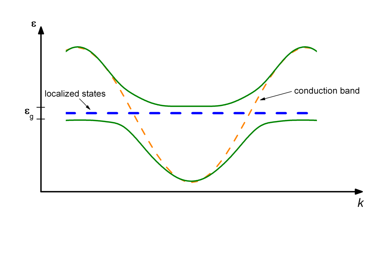
(d) Kondo lattice

Figure 4: (a-c) Formation process of bent flat band by as we change the stregnth of the coupling. From the left to right $B_{xyc}=0,5,10$. The chemical potential is fixed to be $\mu=2\sqrt{3}$. (d) Formation of flat band by hybridization of localized state and conducting state.

4.2 Spectral Function (SF) with Scalar interaction

4.2.1 parity symmetry breaking case : ${\cal L}_{int}=\Phi_{5}({\bar{\psi}}_{1}\Gamma^{5}\psi_{2}+{\bar{\psi}}_{2}\Gamma^{5}\psi_{1})$

We begin with the simplest case where the order parameter field is scalar field. We choose $m_{\Phi}^{2}=-2$ in $AdS_{4}$ for simplicity. Then erlich2005qcd ; oh2019holographic

$$\Phi_{5}=M_{05}z+M_{5}z^{2},$$ (40)

in the probe limit. We consider source only and condensation only cases separately.

Scalar Source: $M_{05}$

The scalar source is usually interpreted as a mass of the boundary fermion. Indeed our result given in the Figure 5(a), where we draw the spectral function (SF) in the presence of scalar with source term only, fulfill such expectation.

(a) $\Phi_{5}$, s

(b) $\Phi_{5}$, c

(c) $\Phi$, s

(d) $\Phi$. s

(e) $B_{r},B_{5r}$, s, c

Figure 5: Spectral Function(SF) (a,b) with parity breaking scalar. (a) with source only. Gap $\Delta\sim M_{05}$. (b) with condensation only, $\Delta\sim\sqrt{M_{5}}$; (c,d) with parity invariant scalar. Notice the zero modes. (c) source only (d) condensation only. (e) $B_{r},B_{rt}$ shows the spectrum of zero coupling due to the gamma matrix structrure.

Scalar Condensation: $M_{5}$.

This case describes the spontaneous scalar condensation. For complex $\Phi$ with nonzero $M$ it describe the cooper pair condensation while for real case it may describe a chiral condensation or a random spin singlet condensation where lattice spins pair up to form singlets, the dimers, in random direction so that there is no net magnetic ordering. In fact, in lattice models with antiferromagnetic coupling, the ground state is anti-ferromagneticaly ordered if frustrations and randomness are small enough. On the other hand, it has random singlet (RS) statebhatt1982scaling ; paalanen1988thermodynamic ; PhysRevLett.48.344 ; guo1994quantum if there is a randomness, a distribution of next-nearest site couplings. Whether a RS like state has a gap or not depends on the details of the lattice symmetry as well as the size of the randomness PhysRevX.8.031028 ; PhysRevB.98.054422 ; Uematsu_2018 ; Liu_2018 ; PhysRevLett.123.087201 ; Kawamura_2019 ; Im . Our philosophy is to bypass all such details and characterize the system only by a few order parameter, assuming this is possible at least near the critical points. From our calculation, a RS state with gap is described by a scalar order. Notice that the dipole type interaction $F_{rt}{\bar{\psi}}\gamma^{rt}\psi$, which was used to study the Mott physics Edalati:2010ww ; Edalati:2010ge ; Seo:2018hrc , does not generate a true gap, because its density of state does not really has a gap although its spectral function has gap like features in small momentum region. This is because the spectral function shows a band that approaches to the fermi level for large momentum.

Spectrum in potential picture

More characteristic feature is the appearance of Kaluza-Klein (KK) modes in the Figure 5, which is due to the effective $z^{2}$ Schrödinger potential for large $z$ generated by the condensation part: the effective Schrödinger potential $V\sim\Phi_{5}^{2}/z^{2}$ which goes like $\sim M_{5}^{2}z^{2}$ for large $z$ oh2019holographic . Comparing the effect of the scalar condensation with that of the scalar source, the gap is generated by condensation is smaller than that generated by the source, as shown in 5 (a,b).

In the presence of chemical potential or temperature, the effect of $z^{2}$ term is suppressed because both $T$ and $\mu$ increase the horizon size $r_{0}$ and the region ’inside’ the black hole, $z>z_{0}=1/r_{0}$ is cut out. Then the rising potential $z^{2}$ also disappear, and the potential near the horizon collapses into $-\infty$ because near the horizon,

$$V_{eff}(z_{H})\sim-\frac{4+w^{2}{z_{H}}^{2}}{16(z-z_{H})^{2}},$$ (41)

Furthermore the solution should satisfy the infalling boundary condition, so that instead of the infinitely many clean quantized eigenvalues (KK modes), only finitely many imaginary eigenvalues due to the tunneling to the horizon appears. See figure 6. This explains the fuzziness and disappearance of KK modes in 5(d) in the presence of the chemical potential.

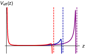
Figure 6: Shape of potential near the horizon. Dashed lines are the event horizons at a few temperatures. As T increases, horizon moves out in $z$-coordinate.

For the vector and tensor cases, there can be a pole between the horizon and the boundary.

We emphasize that this case is not related to the rotational symmetry breaking. The $Z_{2}$ symmetry is not encoded in this model either. So one natural candidate is the spin liquid with a gapFu_2015 ; Oh:2018wfn . This case may be also useful to describe the coupling between the localized (lattice) spin net work and the itinerant electron, namely the Kondo physics.

4.2.2 Parity preserving Scalar interaction : ${\cal L}_{int}=i\Phi({\bar{\psi}}_{1}\psi_{2}+{\bar{\psi}}_{2}\psi_{1})$

For the consistency with scalar model, we choose the $m_{\Phi}^{2}=-2$ so that we still have $\Phi=M_{0}z+Mz^{2}$. The spectrum is gapped for both source and condensation. For the latter case zero chemical potential case shows sharp KK modes. Compared with the scalar case, spectrum is sharper. See Figure 5 (c,d) for the spectral functions with pseudo scalar source and condensation respectively. The system is similar to the scalar but with Parity symmetry broken. The most famous case is the pion condensation in nuclear physics.

4.3 Vectors

From the 2+1 dimension boundary point of view there are three classes of vectors: $B_{\mu},B_{r\mu}$ and $B_{5\mu}$, respectively. In each class, the source shifts the two degenerate Dirac cones, one to negative and the other to positive $k_{\mu}$ directions. The last two classes are invariant under the parity showing zero mode related feature like Fermi-arc and surface states(Ribbon band). See figures 8, and 7.

4.3.1 Polar Vector: ${\cal L}_{int}=\boldmath{iB_{\mu}}({\bar{\psi}}_{1}\Gamma^{\mu}\psi_{2}-{\bar{\psi}}_{2}\Gamma^{\mu}\psi_{1})$

$B_{\mu}$ is the extension of the source field that couples to boundary fermion current ${\bar{\chi}}\Gamma^{\mu}\chi$. We can set the mass of vector and axial-vector order field to zero. Then, $B_{i}=B^{(0)}_{i}+B^{(1)}_{i}z^{1}$. Notice that there are asymmetry between $x$ and $y$ direction. Therefore when $B_{x}\rightarrow B_{y}$, it has to be followed by $k_{x}\to k_{y}$ at the same time.

Source

SF for $B_{x}$ coupling with source only is just superposition of two shifted SF’s of zero coupling cases along the $k_{x}$. Different flavors shift in opposite directions.

Condensation

: Anisotropy instead of cone splitting is created. See Figure and 7 and 8 .

4.3.2 pseudo Vector: ${\cal L}_{int}=\boldmath{iB_{5\mu}}({\bar{\psi}}_{1}\Gamma^{5\mu}\psi_{2}-{\bar{\psi}}_{2}\Gamma^{5\mu}\psi_{1})$

Pseudo vectors mostly follows the pattern of polar vectors. One important point to emphasize is the line shaped zero mode at $\omega=0$ plane. At higher slice $\omega=2$, there are also lines connecting two cicles representing the two shifted Dirac cones. See figure 7(b)(c). So the total 3 dimensional figure is like Figure 3 with double of the surface modes, which we call Ribbon bands.

4.3.3 radial Vector: ${\cal L}_{int}=\boldmath{iB_{r\mu}}({\bar{\psi}}_{1}\Gamma^{r\mu}\psi_{2}-{\bar{\psi}}_{2}\Gamma^{r\mu}\psi_{1})$

Radial vectors follows the pattern of polar vectors including zero modes. See Figure 8 and 7.

(a) $B_{x}$ s

(b) $\omega=0$, $B_{x}$ s

(c) $\omega=2$, $B_{x}$ s

(d) $B_{x}$ c

(e) $\omega=0$, $B_{x}$ c

(f) $\omega=2$, $B_{x}$ c

(g) $B_{5x}$ s

(h) $\omega=0$, $B_{5x}$ s

(i) $\omega=2$, $B_{5x}$ s

(j) $B_{5x}$ c

(k) $\omega=0$, $B_{5x}$ c

(l) $\omega=2$, $B_{5x}$ c

Figure 7: (adgj)Spectral Functions of $B_{x}$ and $B_{5x}$ with additional sliced view in $k_{x},k_{y}$ plane of $\omega=0,2$ slices. Notice that source splits the degenerated Dirac cones. $B_{x}$ has zero modes nut $B_{5x}$ does not. In all figures, we used $B_{*}=4$.

(a) s, $B_{5t(0)}$

(b) $\omega=0$, $B_{5t}s$

(c) s, $B_{5y(0)}$

(d) s, $B_{t(0)}$

(e) $\omega=0$, $B_{t}s$

(f) s, $B_{y(0)}$

(g) c, $B_{5t(0)}$

(h) $\omega=0$, $B_{5t}c$

(i) c, $B_{5y(0)}$

(j) c, $B_{t(0)}$

(k) $\omega=0$, $B_{t}c$

(l) c, $B_{y(0)}$

Figure 8: Spectral function with (pseudo) vector source interactions (a-f), and SF with (pseudo)-vector condensation (g-l). s means source and c means condensation.

4.4 Antisymmetric 2-Tensor

6 anti-symmetric rank 2 tensors can be decomposed into three $B_{\mu r},\mu=0,1,2$ and the rests $B_{tx},B_{ty},B_{xy}$. The former was already described above.

Notice the manifest zero mode Disk in $B_{tr}$ from the figure 9. There are rotational symmetry in $B_{tr},B_{xy}$, but notin $B_{xr}$. Spectrum of $B_{ty}$ and $B_{xr}$ are ambiguous without the views in $k_{x}$-$k_{y}$ at various $\omega$ slices, which we provide in figure 10. Both of them have split cones and the zero modes. Both have Ribbon bands connecting the two cones.

(a) $B_{xy(-1)}$ s

(b) $B_{xy(-1)}$ s

(c) $B_{xy(0)}$ c

(d) $B_{tr(-1)}$ s

(e) $B_{tr(0)}$ c

(f) $B_{tr(0)}$ c

Figure 9: Spectral function with various types tensor interaction, which is decomposed into 2+1 radial vector $B_{\mu r}$’s (ab) and 2-tensor $B_{xy}$ (cd). Notice the zero mode Disk in $B_{xy}$. There are rotational symmetry in $B_{tr},B_{xy}$.

(a) $B_{ty(0)}$ s

(b) $\omega=0$ $B_{ty}$ s

(c) $\omega=2$ $B_{ty}$ s

(d) c, $B_{ty(0)}$

(e) $\omega=0$ $B_{ty}$ c

(f) $\omega=2$ $B_{ty}$ c

(g) $B_{rx(0)}$ s

(h) $\omega=0$ $B_{rx}$ s

(i) $\omega=2$ $B_{rx}$ s

(j) c, $B_{rx(0)}$

(k) $\omega=0$ $B_{rx}$ c

(l) $\omega=2$ $B_{rx}$ c

Figure 10: Spectrum of $B_{rx}$ and $B_{ty}$ with sliced views $k_{x}$-$k_{y}$ at $\omega=0,2$ slices, without which these spectra are ambiguous. Notice the zero modes and Ribbons connecting the two split cones.

5 Conclusion

We classified the Yukawa type interactions according to its Lorentz symmetry of the boundary theory and calculate their spectral functions. We met many interesting features that appear in the strongly correlated system: gap, pseudogap, flat band and Fermi-arc stuctures appear.

Out of the 16 interaction types, only parity breaking scalar interaction ($\Gamma=\mathbb{1}$) creates a gap without ambiguity. Both source and the condensation create gaps. However, the parity conserving scalar ($\Gamma=\Gamma^{5}$) has a zero mode Dirac cone in spectrum, which is much sharper than the case of the non-interacting case due to the transfer of the spectral weight to the zero mode by the interaction. The genuine physical system with full gap will be described by this coupling. For vector $B_{\mu}$, $B_{5\mu}$, $B_{r\mu}$ show feature of split cones if the order parameter field have source part. The last two are invariant under the parity , there are the Fermi-arc. Another interesting feature is the flat disk band of $B_{xy}$, which might be useful to describe the twisted bi-layered graphene. If chemical potential is applied, the disk bend like a bowl and the fermi level shifts, resembling the band of the Kondo lattice.

There are three classes of vectors, $B_{\mu},B_{r\mu}$ and $B_{5\mu}$, respectively. The source creates the splited cones and the condensation creates just asymmetry. The first two are invariant under the reflection showing zero mode related features like Fermi-arc and surface states(Ribbon band). There are 3 tensor types: $\Gamma^{xy},\Gamma^{tx},\Gamma^{ty}$. These respect the parity and has zero modes.

Since the spectral data is the fingerprint of a matter, we would be able to determine the order of a strongly interacting system by comparing the calculated spectral function in the presence of these orders with the experimental data. We expect that our result will give an insight for magnetic orders of strongly interacting materials.

Final remark is that the quartic or higher terms do not contribute to the spectral functions.Therefore it is enough to discuss the effect of the Yukawa coupling to calculate the leading order effects of order parameter fields on the fermion spectrum. In fact, the Yukawa coupling terms are most relevant ones in low energy. Here we consider the gravity background of asymptotically AdS4 with Lorentz invariance.

In the future, we will study the AdS₅ version of this paper, which related to Weyl Semi-metal instead of Dirac semi-metal. It will be also interesting to extend our work to higher quantum critical points. There are ten classes of different topological insulator/superconductors depending on the discrete symmetries. It will be also interesting to realize all of such 10 folds way in terms of the explicit laglangian. One more possibility is to study the effect of combinations of the Yukawa interactions to create different types of spectral features. Studies in these directions are under progress.

Appendix A spectrum with one flavour

We present the results for 1 flavor, which in many case seems to give an half of the 2-flavor case with an asymmetry.

A.1 Scalar

(a) s $M_{0}$

(b) s $M_{5}$

(c) c $M_{0}$

(d) c $M_{5}$

Figure 11: SF (a) with scalar source, Gap $\Delta\sim M_{0}$. (b) with pseudo-scalar source. Gap $\Delta\sim\sqrt{M}$. (c) with scalar condensation (d) with pseudo-scalar condensation.

Other type of scalars $\Gamma^{r5},\Gamma^{r}$ does not seem to change the spectrum of zero scalar coupling. Notice that there is no zero mode in one flavor scalar interaction. This is striking difference from the 2 flavor case.

A.2 Vectors

(a) s, $B_{x}$

(b) $\omega=0$, $B_{x}$ s

(c) $\omega=2$, $B_{x}$ s

(d) c, $B_{x}$

(e) $\omega=0$, $B_{x}$ c

(f) $\omega=2$, $B_{x}$ c

(g) s, $B_{5x}$

(h) $\omega=0$, $B_{5x}$ s

(i) $\omega=2$, $B_{5x}$ s

(j) c, $B_{5x}$

(k) $\omega=0$, $B_{5x}$ c

(l) $\omega=2$, $B_{5x}$ c

Figure 12: SF with most typical vector interactions

(a) s, $B_{t(0)}$

(b) s, $B_{y(0)}$

(c) s, $B_{5t(0)}$

(d) s, $B_{5y(0)}$

(e) c, $B_{t(0)}$

(f) c, $B_{y(0)}$

(g) c, $B_{5t(0)}$

(h) c, $B_{5y(0)}$

Figure 13: SF with various types vector condensation interaction

A.3 Anti-symmetric Tensor

(a) s, $B_{ty(0)}$

(b) $\omega=0$ $B_{ty}$ s

(c) $\omega=2$ $B_{ty}$ s

(d) c, $B_{ty(0)}$

(e) $\omega=0$ $B_{ty}$ c

(f) $\omega=2$ $B_{ty}$ c

(g) s, $B_{xr(0)}$

(h) $\omega=0$ $B_{xr}$ s

(i) $\omega=2$ $B_{xr}$ s

(j) c, $B_{xr(0)}$

(k) $\omega=0$ $B_{xr}$ c

(l) $\omega=2$ $B_{xr}$ c

(m) s, $B_{xy}$

(n) s, $B_{tr}$

(o) c, $B_{xy}$

(p) c, $B_{tr}$

Figure 14: Spectrum of Anti-symmetric tensors.

Appendix B The role of the chemical potential

Let’s begin by looking at the simplest scalar case. As one can see from figure 15, the main effect of the chemical potential is three folds: the first is to shift the Fermi-level and the second is to make the spectrum fuzzier. The third one is to introduce the asymmetry between the positive and negative frequency regions.

(a) $\mu=0$, $A(w,k)$

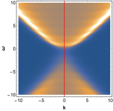
(b) $\mu=2\sqrt{3}$, $A(w,k)$

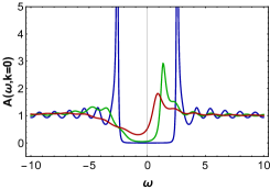
(c) $A(w,k=0)$

Figure 15: The role of $\mu$ for the case with scalar condensation : (a) without and (b) with chemical potential. (c) Spectrum at $k=0$: blue for $\mu=0$, green for $\mu=\sqrt{3}$, red for $\mu=2\sqrt{3}$.

Now we consider the one flavor $B_{xy}$ and $B_{tr}$ interactions which are in a sense dual to each other. To consider the case of spontaneously broken symmetry, we set $B_{(-1)}=0$. Most important feature here is the appearance of the flat band and gated gap, which means that the gap is reachable by gating. For $\mu=0$, exact flat band is generated at $w=0$. If we turn on the chemical potential, the central flat band is bent to give a shallow-bowl shaped band. With increasing A fuzzy flat band is created at higher energy. See Figure 16(d). Notice the similarity of the spectrum with that of the heavy fermion spectrum in Kondo lattice, where an impurity spin interact with the itinerant electron with anti-ferromagnetic coupling. Indeed, our interaction term $\boldmath{B_{xy}}{\bar{\psi}}\Gamma^{xy}\psi$ is the form of the Kondo coupling $\boldmath{\vec{S}_{imp}}\cdot{\bar{\psi}}\vec{\sigma}\psi$ in the boundary if we interpret the order parameter field $B_{xy}$ as the impurity spin along $z$ axis, because $\Gamma^{xy}$ is the corresponding spin generator matrix.

(a) $B_{xy}$ s, $\mu=0$

(b) $B_{xy}$ s, $\mu=\sqrt{3}$

(c) $B_{xy}$ c, $\mu=0$

(d) $B_{xy}$ c, $\mu=\sqrt{3}$

Figure 16: (a,b): SF with only source $B_{xy}$ with one flavor. Notice the presence of the flat band of disk-shape, which is bent down in the presence of chemical potential; (c,d): SF with only condensation $B_{xy}$. All figures here have cylindrical symmetry.

Both source and condensation seem to develop a gap in the negative energy region while Fermi level passes through the conduction band. Since gap usually means gap containing the Fermi-level to give an insulator, we need a new name. We call such gap as gated gap because we expect that we can get an insulator by gating the system, that is by applying external electric field. Therefore we studied the evolution of $B_{rt}$ in $\mu$. Figure 18 shows, however, that gap is generated only in a window of negative $\mu$ around $\mu=-1$.

(a) $\mu=-2\sqrt{3}$

(b) $\mu=-\sqrt{3}$

(c) $\mu=0$

(d) $\mu=\sqrt{3}$

(e) $\mu=2\sqrt{3}$

(f) $\mu=-2\sqrt{3}$ to $\mu=2\sqrt{3}$

Figure 17: $\mu$-evolution of SF of $B_{rt}$ interaction with condensation $B_{rt(0)}=7$. (a,b,c,d,e): denisity plot in $(\omega,k)$. (f):SF at the Fermi level. The minimum of DOS is at $\mu\simeq-1$.

B.1 $B_{rt}$ vs $F_{rt}$:

We want to make a comment on comparing this case with the work of Phillips et.alEdalati:2010ww ; Edalati:2010ge where the dipole interaction $F_{rt}{\bar{\psi}}\Gamma^{rt}\psi$ was considered in search of the gap. The difference with ours is that our $B_{rt}$ is an order parameter independent of the basic vector field $A_{\mu}$ while $F_{rt}=\partial_{r}A_{t}$. Namely,

$$A =\mu_{1}-\frac{r_{0}}{r})dt,\quad F=dA=\frac{\mu r_{0}}{r^{2}}dt\wedge dr,\quad B=B^{(0)}_{rt}dt\wedge dr.$$ (42)

If the condensation $B^{(0)}_{rt}$ is related to the chemical potential by $B^{(0)}_{rt}=\mu/r_{0}$, our model with non-zero chemical potential is exactly the same as the dipole interaction model. In fact, Figure 18 shows that the overall features of two cases are similar. However, for zero chemical potential, our model still have the non-zero order parameter $B^{(0)}_{rt}$ while the dipole interaction vanishes automatically.

(a) $\mu=\sqrt{3},F_{rt}$

(b) $\mu=2\sqrt{3},F_{rt}$

(c) $\mu=\sqrt{3},B_{rt}$

(d) $\mu=2\sqrt{3},B_{rt}$

Figure 18: (a,b): SF for $F_{rt}$ and (c,d): SF for $B_{rt}$ with condensation $B^{(0)}_{rt}=7$. Two models are similar.

Both source and condensation seem to develop a gap in the negative energy region while Fermi level passes through the conduction band. Since gap usually means gap containing the Fermi-level to give an insulator, we need a new name. We call such gap as gated gap because we expect that we can get an insulator by gating the system, that is by applying external electric field. Therefore we studied the evolution of $B_{rt}$ in $\mu$. Figure 18 shows, however, that gap is generated only in a window of negative $\mu$ around $\mu=-1$.

- (1) J. Crossno, J. K. Shi, K. Wang, X. Liu, A. Harzheim, A. Lucas et al., Observation of the Dirac fluid and the breakdown of the Wiedemann-Franz law in graphene, Science 351 (Mar., 2016) 1058–1061, [1509.04713].
- (2) A. Lucas, J. Crossno, K. C. Fong, P. Kim and S. Sachdev, Transport in inhomogeneous quantum critical fluids and in the Dirac fluid in graphene, Phys. Rev. B93 (2016) 075426, [1510.01738].
- (3) M. Liu, J. Zhang, C.-Z. Chang, Z. Zhang, X. Feng, K. Li et al., Crossover between weak antilocalization and weak localization in a magnetically doped topological insulator, Phys. Rev. Lett. 108 (2012) 036805.
- (4) D. Zhang et al., Interplay between ferromagnetism, surface states, and quantum corrections in a magnetically doped topological insulator, Physical Review B 86 (2012) 205127.
- (5) L. Bao, W. Wang, N. Meyer, Y. Liu, C. Zhang, K. Wang et al., Quantum corrections crossover and ferromagnetism in magnetic topological insulators, Scientific reports 3 (2013) .
- (6) Y. Seo, G. Song, P. Kim, S. Sachdev and S.-J. Sin, Holography of the Dirac Fluid in Graphene with two currents, Phys. Rev. Lett. 118 (2017) 036601, [1609.03582].
- (7) Y. Seo, G. Song and S.-J. Sin, Strong Correlation Effects on Surfaces of Topological Insulators via Holography, Phys. Rev. B96 (2017) 041104, [1703.07361].
- (8) Y. Seo, G. Song, C. Park and S.-J. Sin, Small Fermi Surfaces and Strong Correlation Effects in Dirac Materials with Holography, JHEP 10 (2017) 204, [1708.02257].
- (9) P. Coleman, Heavy Fermions and the Kondo Lattice: a 21st Century Perspective, 2015. 1509.05769.
- (10) Y. Cao, V. Fatemi, S. Fang, K. Watanabe, T. Taniguchi, E. Kaxiras et al., Unconventional superconductivity in magic-angle graphene superlattices, Nature 556 (2018) 43–50.
- (11) Y. Cao, V. Fatemi, A. Demir, S. Fang, S. L. Tomarken, J. Y. Luo et al., Correlated insulator behaviour at half-filling in magic-angle graphene superlattices, Nature 556 (2018) 80.
- (12) K. G. Wilson, Renormalization group and critical phenomena. i. renormalization group and the kadanoff scaling picture, Physical review B 4 (1971) 3174.
- (13) K. G. Wilson, The renormalization group: Critical phenomena and the kondo problem, Reviews of modern physics 47 (1975) 773.
- (14) J. M. Maldacena, The Large N limit of superconformal field theories and supergravity, Int.J.Theor.Phys. 38 (1999) 1113–1133, [hep-th/9711200].
- (15) E. Witten, Anti-de Sitter space and holography, Adv. Theor. Math. Phys. 2 (1998) 253–291, [hep-th/9802150].
- (16) S. S. Gubser, I. R. Klebanov and A. M. Polyakov, Gauge theory correlators from noncritical string theory, Phys. Lett. B428 (1998) 105–114, [hep-th/9802109].
- (17) E. Alvarez and C. Gomez, Geometric holography, the renormalization group and the c-theorem, arXiv preprint hep-th/9807226 (1998) .
- (18) V. Balasubramanian and P. Kraus, Spacetime and the holographic renormalization group, Physical Review Letters 83 (1999) 3605.
- (19) J. De Boer, E. Verlinde and H. Verlinde, On the holographic renormalization group, Journal of High Energy Physics 2000 (2000) 003.
- (20) I. Heemskerk and J. Polchinski, Holographic and wilsonian renormalization groups, Journal of High Energy Physics 2011 (2011) 31.
- (21) E. Fradkin, Field theories of condensed matter physics. Cambridge University Press, 2013.
- (22) S.-S. Lee, A Non-Fermi Liquid from a Charged Black Hole: A Critical Fermi Ball, Phys. Rev. D79 (2009) 086006, [0809.3402].
- (23) H. Liu, J. McGreevy and D. Vegh, Non-Fermi liquids from holography, Phys. Rev. D83 (2011) 065029, [0903.2477].
- (24) N. Iqbal and H. Liu, Real-time response in AdS/CFT with application to spinors, Fortsch. Phys. 57 (2009) 367–384, [0903.2596].
- (25) M. Cubrovic, J. Zaanen and K. Schalm, String Theory, Quantum Phase Transitions and the Emergent Fermi-Liquid, Science 325 (2009) 439–444, [0904.1993].
- (26) T. Faulkner, G. T. Horowitz, J. McGreevy, M. M. Roberts and D. Vegh, Photoemission ’experiments’ on holographic superconductors, JHEP 03 (2010) 121, [0911.3402].
- (27) F. Benini, C. P. Herzog and A. Yarom, Holographic fermi arcs and a d-wave gap, Physics Letters B 701 (2011) 626–629.
- (28) D. Vegh, Fermi arcs from holography, 1007.0246.
- (29) M. Edalati, R. G. Leigh and P. W. Phillips, Dynamically Generated Mott Gap from Holography, Phys. Rev. Lett. 106 (2011) 091602, [1010.3238].
- (30) M. Edalati, R. G. Leigh, K. W. Lo and P. W. Phillips, Dynamical Gap and Cuprate-like Physics from Holography, Phys. Rev. D83 (2011) 046012, [1012.3751].
- (31) J. N. Laia and D. Tong, A holographic flat band, Journal of High Energy Physics 2011 (2011) 125.
- (32) V. Alexandrov and P. Coleman, Spin and holographic metals, Phys. Rev. B 86 (2012) 125145, [1204.6310].
- (33) S. A. Hartnoll, C. P. Herzog and G. T. Horowitz, Building a Holographic Superconductor, Phys.Rev.Lett. 101 (2008) 031601, [0803.3295].
- (34) S. S. Gubser, Breaking an Abelian gauge symmetry near a black hole horizon, Phys.Rev. D78 (2008) 065034, [0801.2977].
- (35) N. Armitage, E. Mele and A. Vishwanath, Weyl and Dirac Semimetals in Three Dimensional Solids, Rev. Mod. Phys. 90 (2018) 015001, [1705.01111].
- (36) J. Erlich, E. Katz, D. T. Son and M. A. Stephanov, Qcd and a holographic model of hadrons, Physical Review Letters 95 (2005) 261602.
- (37) E. Oh and S.-J. Sin, Holographic abelian higgs model and the linear confinement, arXiv preprint arXiv:1909.13801 (2019) .
- (38) R. N. Bhatt and P. Lee, Scaling studies of highly disordered spin- antiferromagnetic systems, Physical Review Letters 48 (1982) 344.
- (39) M. Paalanen, J. Graebner, R. N. Bhatt and S. Sachdev, Thermodynamic behavior near a metal-insulator transition, Physical review letters 61 (1988) 597.
- (40) R. N. Bhatt and P. A. Lee, Scaling studies of highly disordered spin-½ antiferromagnetic systems, Phys. Rev. Lett. 48 (Feb, 1982) 344–347.
- (41) M. Guo, R. N. Bhatt and D. A. Huse, Quantum critical behavior of a three-dimensional ising spin glass in a transverse magnetic field, Physical review letters 72 (1994) 4137.
- (42) I. Kimchi, A. Nahum and T. Senthil, Valence bonds in random quantum magnets: Theory and application to , Phys. Rev. X 8 (Jul, 2018) 031028.
- (43) M. Watanabe, N. Kurita, H. Tanaka, W. Ueno, K. Matsui and T. Goto, Valence-bond-glass state with a singlet gap in the spin- square-lattice random heisenberg antiferromagnet , Phys. Rev. B 98 (Aug, 2018) 054422.
- (44) K. Uematsu and H. Kawamura, Randomness-induced quantum spin liquid behavior in the s=12 random j1−j2 heisenberg antiferromagnet on the square lattice, Physical Review B 98 (Oct, 2018) .
- (45) L. Liu, H. Shao, Y.-C. Lin, W. Guo and A. W. Sandvik, Random-singlet phase in disordered two-dimensional quantum magnets, Physical Review X 8 (Dec, 2018) .
- (46) K. Uematsu and H. Kawamura, Randomness-induced quantum spin liquid behavior in the random-bond heisenberg antiferromagnet on the pyrochlore lattice, Phys. Rev. Lett. 123 (Aug, 2019) 087201.
- (47) H. Kawamura and K. Uematsu, Nature of the randomness-induced quantum spin liquids in two dimensions, Journal of Physics: Condensed Matter 31 (sep, 2019) 504003.
- (48) e. Im, Pseudo-gaps and the condensation of singlets in a degenerately doped silicon metal, submitted to nature (2020) .
- (49) Y. Seo, G. Song, Y.-H. Qi and S.-J. Sin, Mott transition with Holographic Spectral function, 1803.01864.
- (50) M. Fu, T. Imai, T.-H. Han and Y. S. Lee, Evidence for a gapped spin-liquid ground state in a kagome heisenberg antiferromagnet, Science 350 (Nov, 2015) 655–658.
- (51) E. Oh and S.-J. Sin, Entanglement String and Spin Liquid with Holographic Duality, 1811.07299.