Measurement Clusterization in D-optimal Designs for Bayesian Linear Inverse Problems over Hilbert Spaces

Abstract.

Inversion for parameters of a physical process typically requires taking expensive measurements, and the task of finding an optimal set of measurements is known as the optimal design problem. Surprisingly, measurement locations in optimal designs are sometimes extremely clustered, and researchers often avoid measurement clusterization by modifying the optimal design problem. We consider a certain flavor of the optimal design problem, based on the Bayesian D-optimality criterion, and suggest an analytically tractable model for D-optimal designs in Bayesian linear inverse problems over Hilbert spaces. We demonstrate that measurement clusterization is a generic property of D-optimal designs, and prove that correlated noise between measurements mitigates clusterization. We also give a full characterization of D-optimal designs under our model: We prove that D-optimal designs uniformly reduce uncertainty in a select subset of prior covariance eigenvectors. Finally, we show how measurement clusterization is a consequence of the characterization mentioned above and the pigeonhole principle.

1. Introduction

Measurements play a fundamental role in generating observations and are indispensable to any inference process. In the realm of data science, selecting the optimal set of measurements holds particular significance when inferring parameters of a physical process. Unlike many other fields, where measurements are fixed, in this context, we have the freedom to choose which measurements to take. This freedom should be taken advantage of: measurements should be chosen to enhance accuracy, reduce costs, or both. Whether measurements involve specifying electrode locations on the skin in electric impedance tomography [16], determining certain wavelengths in MRI [22], or positioning sensors for detecting ground-reflected waves in the search for oil [15], the selection of optimal measurements, referred to as the problem of optimal design, becomes crucial. Optimal measurements are chosen according to specific design criteria, with A- and D-optimality being two of the most widely recognized and extensively studied design criteria [9].

Surprisingly, A- and D-optimal designs have been observed to yield remarkably similar measurements in certain cases [13, 24, 14, 27, 23]. To illustrate this point, we consider a toy inverse problem: inferring the initial condition of the 1D heat equation (details in the supplementary material). In Figure 1 D-optimal measurement locations are shown for different numbers of measurements. Notably, for six measurements, a D-optimal design yields two sets of measurements that are almost indistinguishable from one another. We refer to this intriguing phenomenon as measurement clusterization [27], and we refer to a design that exhibits measurement clusterization as a clustered design.

Figure 1. Measurement clusterization for optimal designs when inverting for the initial condition of the 1D heat equation (see supplementary material for details). Measurement locations were chosen according to the Bayesian D-optimality criterion of Theorem 2. Measurement locations are plotted over the computational domain $\Omega=[0,1]$ (x-axis), for varying numbers of measurements (y-axis). The colored numbers are measurement indices, plotted for visual clarity. Measurement clusterization already occurs for three measurements: the second measurement (red) is overlaid with the third (green). For five measurements, first (blue) and second (red) measurements are clustered, as well as the fourth (black) and the fifth (magenta).

Researchers widely agree that measurement clusterization is undesirable [13, 24, 14, 27, 23], prompting the exploration of various remedies to address this issue. One approach involves merging close measurements [14]; however, this strategy merely overlooks the phenomenon of measurement clusterization. An alternative solution lies in clusterization-free designs, where measurement locations are deliberately chosen to be distant from one another. This can be achieved by imposing distance constraints between measurements or by introducing correlated errors that account for both observation error and model misspecification [27]. For instance, in the context of time-series analysis for pharmacokinetic experiments, measurement clusterization can be mitigated by incorporating the modeling of auto-correlation time within the noise terms [24].

In spatial problems involving choice of measurements within a domain $\Omega\subseteq\mathbb{R}^{d},d=1,2,3$, many researchers circumvent the problem of measurement clusterization by choosing measurements from a coarse grid in $\Omega$ [19, 4, 6, 2, 3, 5]. This approach incurs a significant computational cost as it requires solving a difficult combinatorial optimization problem for measurement locations over a finite set. The combinatorial optimization problem is usually relaxed by first assigning optimal measurement weights in $\mathbb{R}_{+}$ to the potential measurement locations. Some researchers incorporate a sparsifying $\ell_{1}$ penalty term into the design criterion, which is subsequently thresholded to achieve the desired binary design over the coarse grid [15]. Others progressively relax the $\ell_{1}$ penalty to an $\ell_{0}$ penalty via a continuation method [3, 2]. A clever alternative is to cast the problem of finding optimal measurement weights as a stochastic optimization problem [7]. All of the aforementioned methods may indeed find a binary optimal design restricted to a given coarse grid. However, none addresses one fundamental issue: the restriction of measurement locations to a coarse grid in $\Omega$ fundamentally changes the optimal design problem and thus results in a sub-optimal design.

Avoiding measurement clusterization is a pragmatic approach: intuitively, researchers recognize that measurement clusterization is undesirable, even though the underlying reasons may not be fully clear. Consequently, they strive to prevent it and devise various methodologies to avoid measurement clusterization. Yet each and every one of these methodologies achieves its objective by imposing restrictions on measurement locations, thereby fundamentally altering the optimal design problem. To the best of my knowledge, no previous study has tried to address some seemingly simple yet fundamental questions: Why does imposing correlations between observations alleviate measurement clusterization? Is measure clusterization a generic phenomenon? And, most importantly: Why does measurement clusterization occur?

1.1. Contribution

The primary objective of this study is to provide a comprehensive understanding of measurement clusterization by addressing the aforementioned questions. Our focus centers around investigating the Bayesian D-optimality criterion, which involves maximizing the expected Kullback-Leibler divergence between the posterior and prior measures [11, 9]. We conduct an analysis of Bayesian D-optimal designs within the context of linear inverse problems over Hilbert spaces. We propose a novel relaxed model for D-optimality that maintains analytical tractability and enables the identification of D-optimal designs using Lagrange multipliers. This analytical framework facilitates the exploration of the questions posed at the end of the previous paragraph:

1. Is measurement clusterization a generic phenomenon? Randomized numerical simulations of our model give rise to D-optimal designs that exhibit clusterization more than 95% of the time (see code in supplementary material). Given our model’s genericity, we expect measurement clusterization to be a generic phenomenon.

2. Why does imposing correlations between observations alleviate measurement clusterization? In Section 4, we rigorously demonstrate the role of model error in mitigating clusterization, thereby corroborating earlier observations made by various researchers.

3. Why does measurement clusterization occur? In Section 6, we present a compelling explanation for the optimality of clustered designs in the absence of model error. Our analysis reveals that, in our model, a D-optimal design focuses on a select set of prior eigenvectors, specifically those with the largest eigenvalues in the prior covariance spectrum. In practical scenarios, the number of locations where the relevant prior eigenvectors are significantly large, while other eigenvectors have a power spectrum close to zero, is limited. Consequently, the clustering of measurements arises as a natural consequence of the pigeonhole principle, as there are more measurements available than there are locations satisfying conditions (a) and (b).

The cornerstone of our investigation into measurement clusterization is Theorem 1 proven in Section 5. The key insight of Theorem 1 lies in its fifth component, which highlights that a D-optimal design aims to uniformly reduce posterior uncertainties for posterior covariance eigenvectors in observation space. A similar conclusion was reached by Koval et al. [19], who showed that A-optimal designs are best constructed in the space of observations.

We first give some general definitions before we state Theorem 1: Let $\mathcal{H}_{p},\mathcal{H}_{o}$ Hilbert spaces, $\mathcal{F}:\mathcal{H}_{p}\to\mathcal{H}_{o}$ a linear compact operator. Let $\mathcal{O}:\mathcal{H}_{o}\to\mathbb{R}^{m}$ a linear measurement operator, where $m\in\mathbb{N}$ is the number of measurements taken. Let $\sigma^{2}\in\mathbb{R}_{+}$ observation noise variance, $\mathbf{d}=\mathcal{O}\mathcal{F}\mathbf{m}+\varepsilon$, where $\varepsilon\in\mathbb{R}^{m}$ is iid $\mathcal{N}(0,\sigma^{2})$ noise. Let $\mu_{\textup{pr}}\sim\mathcal{N}(\mathbf{m}_{\textup{pr}},\Gamma_{\textup{pr}})$ prior Gaussian measure on $\mathcal{H}_{p}$, where $\Gamma_{\textup{pr}}$ is the prior covariance operator and let $\mu_{\textup{post}}^{\mathbf{d},\mathcal{O}}$ the posterior (Gaussian) measure.

Theorem 1.

Let:

• The D-optimality design criterion [1]:

  $$\begin{split}\Psi(\mathcal{O})&=\frac{1}{2}\log\det(I+\sigma^{-2}\Gamma_{\textup{pr}}^{1/2}\mathcal{F}^{*}\mathcal{O}^{*}\mathcal{O}\mathcal{F}\Gamma_{\textup{pr}}^{1/2}),\end{split}$$

• $\mathcal{O}$ a D-optimal design operator

  $$\mathcal{O}=\operatorname*{arg\,max}_{\|\mathbf{o}_{j}\|=1,j=1,\dots,m}\Psi(\mathcal{O}),$$

• $\{\lambda_{i}\}_{i=1}^{\infty}$ eigenvalues of $\mathcal{F}\Gamma_{\textup{pr}}\mathcal{F}^{*}$ in decreasing order of magnitude.

• $\{\eta_{i}\}_{i=1}^{\infty}$ eigenvalues of $\mathcal{O}^{*}\mathcal{O}$.

Then:

1. $\textup{tr}\left\{\mathcal{O}^{*}\mathcal{O}\right\}=m$.

2. $\mathcal{O}^{*}\mathcal{O}$ and $\mathcal{F}\Gamma_{\textup{pr}}\mathcal{F}^{*}$ are simultaneously diagonalizable.

3. $k:=\textup{rank}\ \mathcal{O}^{*}\mathcal{O}\leq m$ and

   $$\Psi(\mathcal{O})=\frac{1}{2}\sum_{i=1}^{k}\log(1+\sigma^{-2}\lambda_{i}\eta_{i}).$$

4. $$\eta_{i}=\begin{cases}\frac{m}{k}-\sigma^{2}\lambda_{i}^{-1}+\sigma^{2}\frac{1}{k}\sum_{j=1}^{k}\lambda_{j}^{-1}&1\leq i\leq k\\ 0&i>k\end{cases}.$$

5. The covariance of the pushforwad $\mathcal{F}_{*}\mu_{\textup{post}}^{\mathbf{d},\mathcal{O}}$ is $\left((\mathcal{F}\Gamma_{\textup{pr}}\mathcal{F}^{*})^{-1}+\sigma^{-2}\mathcal{O}^{*}\mathcal{O}\right)^{-1}$ and has eigenvalues

   $$\theta_{i}=\begin{cases}\left(\frac{\sum_{j=1}^{k}\lambda_{j}^{-1}+\sigma^{-2}m}{k}\right)^{-1}&i\leq k\\ \lambda_{i}&i>k\end{cases}$$

In the proving Theorem 1 we prove and generalize several lemmas. Among those, is a Lemma 3, which is (to the the best of my knowledge) a novel lemma in linear algebra: We decompose a symmetric positive definite matrix $M\in\mathbb{R}^{k\times k}$ with $\textup{tr}\ M=m\in\mathbb{N}$ as $M=AA^{t}$, where $A$ has unit norm columns.

1.2. Limitations

The main limitation of this study is that our generic model does not correspond to any specific real-life problem. It is generic enough to be analytically tractable, but one may argue our model is too far removed from any real application. To these claims I would answer that scientists have a long history of studying models that are bare-bones simplifications of real systems, e.g. the Ising model [10], the Lorenz system [8], the Lotka-Volterra equations [21], the Carnot engine [18], and many others.

2. Preliminaries and Notation

In this section we present the setup that will be used throughout this article. The theoretical foundations for inverse problems over function spaces can be found in [25] and will not be reviewed here.

2.1. Bayesian Linear Inverse Problems

Let $\mathcal{H}_{p}$ and $\mathcal{H}_{o}$ be separable Hilbert spaces (the subscripts p and o are for “parameter” and “observation”, respectively), and let $\mathcal{F}:\mathcal{H}_{p}\to\mathcal{H}_{o}$ the forward operator. The forward operator $\mathcal{F}$ is assumed linear and strongly smoothing (the heat operator of the 1D heat equation introduced in Section 1 is a prime example). Take a Gaussian prior $\mathbf{m}\sim\mu_{\textup{pr}}=\mathcal{N}(\mathbf{m}_{\textup{pr}},\Gamma_{\textup{pr}})$ with some appropriate covariance operator $\Gamma_{\textup{pr}}$ on $\mathcal{H}_{p}$ [25]. Note that $\mathcal{F}\Gamma_{\textup{pr}}\mathcal{F}^{*}$ is the prior covariance in $\mathcal{H}_{o}$ [25], and as such, $\mathcal{F}\Gamma_{\textup{pr}}\mathcal{F}^{*}$ is assumed invertible — an assumption which will be used below (and if $\mathcal{F}$ has a nontrivial kernel we utilize Occam’s Razor and ignore said kernel). Measurements are taken via the measurement operator. It is common for the measurement and forward operators to be merged $\mathcal{G}:=\mathcal{O}\mathcal{F}$ [1], but the analysis carried out in the following sections requires that $\mathcal{F}$ and $\mathcal{O}$ are explicitly separated as in [7, 12]. $\mathcal{O}\in(\mathcal{H}_{o}^{*})^{m}$, where $m$ is the number of measurements taken. Entries $\mathbf{o}_{j},j=1,\dots,m$ of the observation operator $\mathcal{O}$ are called measurements:

$$\mathcal{O}u=(\mathbf{o}_{1}(u),\dots,\mathbf{o}_{m}(u))^{t}\in\mathbb{R}^{m},\ u\in\mathcal{H}_{o}.$$

Data is acquired via noisy observations, and we consider two types of error terms: Spatially correlated model error $\varepsilon^{\prime}\sim\mathcal{N}(0,\Gamma_{\textup{model}})$ with $\Gamma_{\textup{model}}$ a covariance operator. Observation error is denoted $\varepsilon\sim\mathcal{N}(0,\sigma^{2}I_{m})$, with $I_{m}\in\mathbb{R}^{m\times m}$ the identity. Both error terms and the prior are assumed independent of each other. Thus, data is acquired via

(1) $$\mathbf{d}:=\mathcal{O}(\mathcal{F}\mathbf{m}+\varepsilon^{\prime})+\varepsilon=\mathcal{O}\mathcal{F}\mathbf{m}+\mathcal{O}\varepsilon^{\prime}+\varepsilon.$$

It is easy to verify that $\mathcal{O}\varepsilon^{\prime}+\varepsilon\in\mathbb{R}^{m}$ is a centered Gaussian random vector with covariance matrix

(2) $$\begin{split}\Sigma(\mathcal{O}):&=\mathbb{E}[(\mathcal{O}\varepsilon^{\prime}+\varepsilon)(\mathcal{O}\varepsilon^{\prime}+\varepsilon)^{t}]=\mathcal{O}\Gamma_{\textup{model}}\mathcal{O}^{*}+\sigma^{2}I_{m},\end{split}$$

where

(3) $$\begin{split}[\mathcal{O}\Gamma_{\textup{model}}\mathcal{O}^{*}]_{ij}&=e_{i}^{t}\mathcal{O}\Gamma_{\textup{model}}\mathcal{O}^{*}e_{j}=\mathbf{o}_{i}(\Gamma_{\textup{model}}\mathbf{o}_{j}).\end{split}$$

Taking $\Gamma_{\textup{model}}=0$ is a common practice [26, 17, 28] and then $\Sigma=\sigma^{2}I_{m}$ is a scalar matrix which does not depend on $\mathcal{O}$.

Finally, it is useful to record that the posterior measure $\mu_{\textup{post}}^{\mathbf{d},\mathcal{O}}$ is Gaussian in this setting and its covariance operator is does not depend on data $\mathbf{d}$ [25]:

(4) $$\Gamma_{\textup{post}}=(\Gamma_{\textup{pr}}^{-1}+\mathcal{F}^{*}\mathcal{O}^{*}\Sigma^{-1}\mathcal{O}\mathcal{F})^{-1}.$$

2.2. Bayesian D-Optimal Designs in Infinite Dimensions

A Bayesian D-optimal design maximizes expected Kullback-Leibler (KL) divergence between posterior $\mu_{\textup{post}}^{\mathbf{d},\mathcal{O}}$ and prior measures $\mu_{\textup{pr}}$. It is useful to first recall the definition of KL divergence [11]:

$$D_{KL}(\mu_{\textup{post}}^{\mathbf{d},\mathcal{O}}||\mu_{\textup{pr}})=\int\log\frac{\text{{d}}\mu_{\textup{post}}^{\mathbf{d},\mathcal{O}}}{\text{{d}}\mu_{\textup{pr}}}(\mathbf{m})\text{{d}}\mu_{\textup{post}}^{\mathbf{d},\mathcal{O}}(\mathbf{m}).$$

The study of D-optimal designs for Bayesian linear inverse problems in infinite dimensions was pioneered by [1, 5]. The main result we will make use of is summarized in our notation below:

Theorem 2 (Alexanderian, Gloor, Ghattas [1]).

Let $\mu_{\textup{pr}}=\mathcal{N}(\mathbf{m}_{\textup{pr}},\Gamma_{\textup{pr}})$ be a Gaussian prior on $\mathcal{H}_{p}$ and let $\mu_{\textup{post}}^{\mathbf{d},\mathcal{O}}=\mathcal{N}(\mathbf{m}_{\textup{post}},\Gamma_{\textup{post}})$ the posterior measure on $\mathcal{H}_{p}$ for the Bayesian linear inverse problem $\mathbf{d}=\mathcal{O}\mathcal{F}\mathbf{m}+\mathcal{O}\varepsilon^{\prime}+\varepsilon$ discussed above. Then

(5) $$\begin{split}\Psi(\mathcal{O}):&=\mathbb{E}_{\mathbf{d}}\left[D_{\text{KL}}(\mu_{\textup{post}}^{\mathbf{d},\mathcal{O}}||\mu_{\textup{pr}})\right]\\ &=\frac{1}{2}\log\det(I+\Gamma_{\textup{pr}}^{1/2}\mathcal{F}^{*}\mathcal{O}^{*}\Sigma^{-1}\mathcal{O}\mathcal{F}\Gamma_{\textup{pr}}^{1/2}).\end{split}$$

Note that in [1, 5], results are stated for $\Sigma=I$ (implied by $\Gamma_{\textup{model}}=0,\sigma^{2}=1$), but the these results also hold for more general covariance matrices [1, p. 681].

Definition 1.

We say $\mathcal{O}^{\star}$ is D-optimal if $\mathcal{O}^{\star}=\operatorname*{arg\,max}_{\mathcal{O}}\Psi(\mathcal{O})$, where entries of $\mathcal{O}\in(\mathcal{H}_{o}^{*})^{m}$ are constrained to some allowed set of measurements in $\mathcal{H}_{o}^{*}$.

For a Bayesian linear model in finite dimensions, with Gaussian prior and Gaussian noise, a D-optimal design minimizes the determinant of the posterior covariance matrix, and this turns out to be a regularized version of the frequentist criterion [9]. Theorem 2 and Definition 1 carry a similar intuition:

$$\begin{split}\Psi(\mathcal{O})&=\frac{1}{2}\log\det(I+\Gamma_{\textup{pr}}^{1/2}\mathcal{F}^{*}\mathcal{O}^{*}\Sigma^{-1}\mathcal{O}\mathcal{F}\Gamma_{\textup{pr}}^{1/2})\text{ by \eqref{eq:objective}}\\ &=\frac{1}{2}\log\det\Big{(}\Gamma_{\textup{pr}}(\Gamma_{\textup{pr}}^{-1}+\mathcal{F}^{*}\mathcal{O}^{*}\Sigma^{-1}\mathcal{O}\mathcal{F})\Big{)}\\ &=\frac{1}{2}\log\det\Gamma_{\textup{pr}}\Gamma_{\textup{post}}^{-1}\text{ by \eqref{eq:postcov}}.\end{split}$$

We think of $\Gamma_{\textup{pr}}$ as constant, so a D-optimal design minimizes a quantity analogous to the posterior covariance determinant, similarly to the finite-dimensional case.

3. The Constrained Optimization Problem of D-Optimal Design

We seek a formulation of the D-optimal design problem via Lagrange multipliers. We first find the gradient of $\Psi$, then we suggest unit-norm constraints on $\mathcal{O}$ and find their gradients. Results of this section are summarized in Theorem 3. First, recall that:

Definition 2.

Let $F$ a real valued function of $\mathcal{O}$. The first variation of $F$ at $\mathcal{O}$ in the direction $V$ is:

$$\delta F(\mathcal{O})V:=\frac{\text{{d}}}{\text{{d}}\tau}\Big{|}_{\tau=0}F(\mathcal{O}+\tau V).$$

Moreover, if

$$\delta F(\mathcal{O})V=\textup{tr}\left\{\nabla F(\mathcal{O})V\right\},$$

then we call $\nabla F(\mathcal{O})$ the gradient of $F$ at $\mathcal{O}$.

Proposition 1.

The gradient of the D-optimality objective $\Psi$ is

$$\nabla\Psi(\mathcal{O})=(I-\Gamma_{\textup{model}}\mathcal{O}^{*}\Sigma^{-1}\mathcal{O})\mathcal{F}\Gamma_{\textup{post}}\mathcal{F}^{*}\mathcal{O}^{*}\Sigma^{-1}$$

Proof.

From the definition of $\Sigma(\mathcal{O})$ (2):

(6) $$\begin{split}\frac{\text{{d}}}{\text{{d}}\tau}\Big{|}_{\tau=0}\Sigma(\mathcal{O}+\tau V)&=\frac{\text{{d}}}{\text{{d}}\tau}\Big{|}_{\tau=0}(\mathcal{O}+\tau V)\Gamma_{\textup{model}}(\mathcal{O}+\tau V)^{*}+\sigma^{2}I\\ &=V\Gamma_{\textup{model}}\mathcal{O}^{*}+\mathcal{O}\Gamma_{\textup{model}}V^{*}.\end{split}$$

Then, using (6):

$$0 =\frac{\text{{d}}}{\text{{d}}\tau}\Big{|}_{\tau=0}I$$

$$=\frac{\text{{d}}}{\text{{d}}\tau}\Big{|}_{\tau=0}\left(\Sigma(\mathcal{O}+\tau V)^{-1}\Sigma(\mathcal{O}+\tau V)\right)$$

$$=\frac{\text{{d}}\Sigma(\mathcal{O}+\tau V)^{-1}}{\text{{d}}\tau}\Big{|}_{\tau=0}\Sigma+\Sigma^{-1}\frac{\text{{d}}\Sigma(\mathcal{O}+\tau V)}{\text{{d}}\tau}\Big{|}_{\tau=0}$$

$$=\frac{\text{{d}}\Sigma(\mathcal{O}+\tau V)^{-1}}{\text{{d}}\tau}\Big{|}_{\tau=0}\Sigma+\Sigma^{-1}(V\Gamma_{\textup{model}}\mathcal{O}^{*}+\mathcal{O}\Gamma_{\textup{model}}V^{*}).$$

Thus:

(7) $$\frac{\text{{d}}\Sigma(\mathcal{O}+\tau V)^{-1}}{\text{{d}}\tau}\Big{|}_{\tau=0} =-\Sigma^{-1}(V\Gamma_{\textup{model}}\mathcal{O}^{*}+\mathcal{O}\Gamma_{\textup{model}}V^{*})\Sigma^{-1}.$$

Let

$$T(\mathcal{O})=\mathcal{O}^{*}\Sigma^{-1}(\mathcal{O})\mathcal{O}.$$

By Leibniz (product) rule and (7):

(8) $$\begin{split}\delta T(\mathcal{O})V&=\frac{\text{{d}}T(\mathcal{O}+\tau V)}{\text{{d}}\tau}\Big{|}_{\tau=0}\\ &=V^{*}\Sigma^{-1}\mathcal{O}-\mathcal{O}^{*}\Sigma^{-1}V\Gamma_{\textup{model}}\mathcal{O}^{*}\Sigma^{-1}\mathcal{O}\\ &\ \ \ -\mathcal{O}^{*}\Sigma^{-1}\mathcal{O}\Gamma_{\textup{model}}V^{*}\Sigma^{-1}\mathcal{O}+\mathcal{O}^{*}\Sigma^{-1}V.\end{split}$$

We now record a lemma which is a generalization of Theorem 4 in Chapter 9 of [20]. Its proof is delegated to the supplementary material.

Lemma 1.

Let $Y(t)$ be a differentiable operator-valued function. Assume $I+Y(t)$ is invertible, $Y(t)$ self-adjoint and trace-class. Then

$$\frac{\text{{d}}\log\det(I+Y(t))}{\text{{d}}t}=\textup{tr}\left\{(I+Y(t))^{-1}\dot{Y}(t)\right\}.$$

We employ Lemma 1 and calculate the first variation of $\Psi$:

$$\delta\Psi(\mathcal{O})V: =\frac{\text{{d}}}{\text{{d}}\tau}\Big{|}_{\tau=0}\Psi(\mathcal{O}+\tau V)\text{ (Definition \ref{def:var})}$$

$$=\frac{1}{2}\frac{\text{{d}}}{\text{{d}}\tau}\Big{|}_{\tau=0}\log\det(I+\Gamma_{\textup{pr}}^{1/2}\mathcal{F}^{*}T(\mathcal{O}+\tau V)\mathcal{F}\Gamma_{\textup{pr}}^{1/2})\text{ (Theorem \ref{thm:d optimality})}$$

$$=\frac{1}{2}\textup{tr}\left\{(I+\Gamma_{\textup{pr}}^{1/2}\mathcal{F}^{*}\mathcal{O}^{*}\Sigma^{-1}\mathcal{O}\mathcal{F}\Gamma_{\textup{pr}}^{1/2})^{-1}\frac{\text{{d}}}{\text{{d}}\tau}\Big{|}_{\tau=0}\Gamma_{\textup{pr}}^{1/2}\mathcal{F}^{*}T(\mathcal{O}+\tau V)\mathcal{F}\Gamma_{\textup{pr}}^{1/2}\right\}\ \text{ (Lemma \ref{lemma:lax})}$$

$$=\frac{1}{2}\textup{tr}\ \Big{\{}\Gamma_{\textup{post}}\mathcal{F}^{*}(V^{*}\Sigma^{-1}\mathcal{O}-\mathcal{O}^{*}\Sigma^{-1}V\Gamma_{\textup{model}}\mathcal{O}^{*}\Sigma^{-1}\mathcal{O}$$

$$\ \ \ -\mathcal{O}^{*}\Sigma^{-1}\mathcal{O}\Gamma_{\textup{model}}V^{*}\Sigma^{-1}\mathcal{O}+\mathcal{O}^{*}\Sigma^{-1}V)\mathcal{F}\Big{\}}\text{ (by \eqref{eq:T})}$$

$$=\textup{tr}\left\{\Gamma_{\textup{post}}\mathcal{F}^{*}(\mathcal{O}^{*}\Sigma^{-1}V-\mathcal{O}^{*}\Sigma^{-1}V\Gamma_{\textup{model}}\mathcal{O}^{*}\Sigma^{-1}\mathcal{O})\mathcal{F}\right\}$$

$$=\textup{tr}\left\{\Gamma_{\textup{post}}\mathcal{F}^{*}\mathcal{O}^{*}\Sigma^{-1}V(I-\Gamma_{\textup{model}}\mathcal{O}^{*}\Sigma^{-1}\mathcal{O})\mathcal{F}\right\}$$

$$=\textup{tr}\left\{V(I-\Gamma_{\textup{model}}\mathcal{O}^{*}\Sigma^{-1}\mathcal{O})\mathcal{F}\Gamma_{\textup{post}}\mathcal{F}^{*}\mathcal{O}^{*}\Sigma^{-1}\right\}.$$

Recalling Definition 2 concludes the proof. ∎

In a real-life optimal design problem we cannot choose any measurement operator $\mathcal{O}\in(\mathcal{H}_{o}^{*})^{m}$. In order to facilitate analysis, we seek reasonable constraints on $\mathcal{O}$ for which finding a D-optimal design is analytically tractable. The following proposition will guide us in finding such constraints.

Proposition 2.

Let $\mathcal{O}=(\mathbf{o}_{1},\dots,\mathbf{o}_{m})^{t}$, $j\in\{1,\dots,m\}$, $\sigma^{2}>0$ and $|\zeta|>1$. Then $\Psi(\mathcal{O})$ increases if we use $\zeta\mathbf{o}_{j}$ in $\mathcal{O}$ instead of $\mathbf{o}_{j}$.

Proof.

Fix $j=1,\dots,m$ and take $V:=e_{j}e_{j}^{t}\mathcal{O}$. For $u\in\mathcal{H}_{o}$:

$$Vu=e_{j}e_{j}^{t}(\mathbf{o}_{1}(u),\dots,\mathbf{o}_{m}(u))^{t}=e_{j}\mathbf{o}_{j}(u)=(0,\dots,0,\mathbf{o}_{j}(u),0,\dots,0)^{t}.$$

We now calculate the variation of $\Psi$ at $\mathcal{O}$ in the direction of $V$. Denote $\mathcal{G}:=\mathcal{F}\Gamma_{\textup{post}}\mathcal{F}^{*}$. From Proposition 1:

$$\delta\Psi(\mathcal{O})V =\textup{tr}\left\{V(I-\Gamma_{\textup{model}}\mathcal{O}^{*}\Sigma^{-1}\mathcal{O})\mathcal{G}\mathcal{O}^{*}\Sigma^{-1}\right\}$$

$$=\textup{tr}\left\{e_{j}e_{j}^{t}\mathcal{O}(I-\Gamma_{\textup{model}}\mathcal{O}^{*}\Sigma^{-1}\mathcal{O})\mathcal{G}\mathcal{O}^{*}\Sigma^{-1}\right\}$$

$$=e_{j}^{t}\mathcal{O}(I-\Gamma_{\textup{model}}\mathcal{O}^{*}\Sigma^{-1}\mathcal{O})\mathcal{G}\mathcal{O}^{*}\Sigma^{-1}e_{j}$$

$$=e_{j}^{t}(I-\mathcal{O}\Gamma_{\textup{model}}\mathcal{O}^{*}\Sigma^{-1})\mathcal{O}\mathcal{G}\mathcal{O}^{*}\Sigma^{-1}e_{j}$$

$$=e_{j}^{t}(\Sigma-\mathcal{O}\Gamma_{\textup{model}}\mathcal{O}^{*})\Sigma^{-1}\mathcal{O}\mathcal{G}\mathcal{O}^{*}\Sigma^{-1}e_{j}$$

$$=\sigma^{2}e_{j}^{t}\Sigma^{-1}\mathcal{O}\mathcal{G}\mathcal{O}^{*}\Sigma^{-1}e_{j}\text{ by \eqref{eq:Sigma} }$$

$$=\sigma^{2}e_{j}^{t}\Sigma^{-1}\mathcal{O}\mathcal{F}\Gamma_{\textup{post}}\mathcal{F}^{*}\mathcal{O}^{*}\Sigma^{-1}e_{j}.$$

Since $\Gamma_{\textup{post}}$ is positive definite, we conclude that $\delta\Psi(\mathcal{O})V>0$. This means that increasing the magnitude of the $j^{\text{th}}$ measurement functional increases $\Psi(\mathcal{O})$. ∎

Proposition 2 implies that it is a good idea to bound the norm of measurements. If, for example, we can take measurements in $span\{\mathbf{o}\}$ for some $\mathbf{o}\neq 0$, then no design achieves a maximum of the q D-optimality criterion, since this criterion is not bounded. In contrast, in any real-life problem where sensors are concerned, the norm of measurements recorded by sensors is always one (of course, point evaluations are not in any Hilbert space of functions we wish to consider):

(9) $$\|\delta_{\mathbf{x}}\|=\sup_{0\neq u\in C(\Omega)}\frac{|\int_{\Omega}u(\mathbf{y})\delta_{\mathbf{x}}(\mathbf{y})\text{{d}}\mathbf{y}|}{\sup|u|}=\sup_{0\neq u\in C(\Omega)}\frac{|u(\mathbf{x})|}{\sup|u|}=1,\forall\mathbf{x}\in\Omega.$$

Thus, it is reasonable to consider measurements with unit $\mathcal{H}_{o}^{*}$ norm. The unit norm constraints can be written as a series of $m$ equality constraints (one for each measurement) on $\mathcal{O}$. We define them and find their gradients in Proposition 3 below:

Proposition 3.

Let

$$\phi_{j}(\mathcal{O}):=\frac{1}{2}\|\mathcal{O}^{*}e_{j}\|_{\mathcal{H}_{p}}^{2}-\frac{1}{2}=0,\ j=1,\dots,m.$$

Then

$$\nabla\phi_{j}(\mathcal{O})=\mathcal{O}^{*}e_{j}e_{j}^{t}.$$

Proof.

$$\delta\phi_{j}(\mathcal{O})V =\frac{1}{2}\lim_{\tau\to 0}\tau^{-1}(\|(\mathcal{O}+\tau V)^{*}e_{j}\|_{\mathcal{H}_{p}}^{2}-\|\mathcal{O}^{*}e_{j}\|_{\mathcal{H}_{p}}^{2})$$

$$=\frac{1}{2}\lim_{\tau\to 0}\tau^{-1}(\langle(\mathcal{O}+\tau V)^{*}e_{j},(\mathcal{O}+\tau V)^{*}e_{j}\rangle_{\mathcal{H}_{p}}-\langle\mathcal{O}^{*}e_{j},\mathcal{O}^{*}e_{j}\rangle_{\mathcal{H}_{p}})$$

$$=\frac{1}{2}\lim_{\tau\to 0}\tau^{-1}(2\tau\langle\mathcal{O}^{*}e_{j},V^{*}e_{j}\rangle_{\mathcal{H}_{p}}+\tau^{2}\langle V^{*}e_{j},V^{*}e_{j}\rangle_{\mathcal{H}_{p}})$$

$$=\langle\mathcal{O}^{*}e_{j},V^{*}e_{j}\rangle_{\mathcal{H}_{p}}$$

$$=\langle V\mathcal{O}^{*}e_{j},e_{j}\rangle_{\mathbb{R}^{m}}$$

$$=e_{j}^{t}V\mathcal{O}^{*}e_{j}$$

$$=\textup{tr}\left\{V\mathcal{O}^{*}e_{j}e_{j}^{t}\right\}.$$

∎

Necessary first-order conditions for D-optimality are found via Lagrange multipliers:

(10) $$\nabla\Psi(\mathcal{O})=\sum_{j=1}^{m}\xi_{j}\nabla\phi_{j}(\mathcal{O})$$

(11) $$\phi_{j}(\mathcal{O})=0,j=1,\dots,m.$$

Substitute the gradients calculated in Propositions 1 and 3 into (10):

(12) $$(I-\Gamma_{\textup{model}}\mathcal{O}^{*}\Sigma^{-1}\mathcal{O})\mathcal{F}\Gamma_{\textup{post}}\mathcal{F}^{*}\mathcal{O}^{*}\Sigma^{-1}=\sum_{j=1}^{m}\xi_{j}\mathcal{O}^{*}e_{j}e_{j}^{t}=(\xi_{1}\mathbf{o}_{1},\dots,\xi_{m}\mathbf{o}_{m}).$$

Letting $\Xi:=\textup{diag}(\xi_{j})$, (12) and (11) are written more compactly as:

Theorem 3 (Necessary conditions for D-Optimality).

Let:

$$\mathcal{O}=\operatorname*{arg\,max}_{\|\mathbf{o}_{j}\|=1,j=1,\dots,m}\Psi(\mathcal{O}).$$

Then:

$$(I-\Gamma_{\textup{model}}\mathcal{O}^{*}\Sigma^{-1}\mathcal{O})\mathcal{F}\Gamma_{\textup{post}}\mathcal{F}^{*}\mathcal{O}^{*}\Sigma^{-1}=\mathcal{O}^{*}\Xi,$$

where $\Xi\in\mathbb{R}^{m\times m}$ is diagonal.

4. Answer to Question 2: Model error mitigates clusterization

We now show that if $\Gamma_{\textup{model}}\neq 0$ clusterization will not occur. It is known that including a model error term mitigates the clusterization phenomenon [27], and here we prove this rigorously. Let $\mathcal{O}=(\mathbf{o}_{1},\dots,\mathbf{o}_{m})^{t}$ and $\widehat{\mathcal{O}}:=(\mathbf{o}_{1},\dots,\mathbf{o}_{m-1})^{t}$. Denote $\widehat{\Sigma}:=\Sigma(\widehat{\mathcal{O}})$ and $\widehat{\Gamma_{\textup{post}}}$ the posterior covariance that arises when $\widehat{\mathcal{O}}$ is utilized as a measurement operator.

Proposition 4 (Increase due to a measurement).

Let $\mathcal{O}=(\mathbf{o}_{1},\dots,\mathbf{o}_{m})^{t}$ and $\widehat{\mathcal{O}}:=(\mathbf{o}_{1},\dots,\mathbf{o}_{m-1})^{t}$. Then

(13) $$\Psi(\mathcal{O})-\Psi(\widehat{\mathcal{O}})=\frac{1}{2}\log\left(1+\frac{\langle\mathcal{F}\widehat{\Gamma_{\textup{post}}}\mathcal{F}^{*}(\widehat{\mathcal{O}}^{*}\widehat{\Sigma}^{-1}\Gamma_{\textup{model}}-I)\mathbf{o}_{m},(\widehat{\mathcal{O}}^{*}\widehat{\Sigma}^{-1}\Gamma_{\textup{model}}-I)\mathbf{o}_{m}\rangle}{\sigma^{2}+\mathbf{o}_{m}\Gamma_{\textup{model}}\mathbf{o}_{m}-\mathbf{o}_{m}\Gamma_{\textup{model}}\widehat{\mathcal{O}}^{*}\widehat{\Sigma}^{-1}\widehat{\mathcal{O}}\Gamma_{\textup{model}}\mathbf{o}_{m}}\right).$$

Proof.

Let

$$\Sigma(\mathcal{O}) =\begin{bmatrix}\Sigma(\widehat{\mathcal{O}})&\widehat{\mathcal{O}}\Gamma_{\textup{model}}\mathbf{o}_{m}\\ \mathbf{o}_{m}\Gamma_{\textup{model}}\widehat{\mathcal{O}}^{*}&\sigma^{2}+\mathbf{o}_{m}\Gamma_{\textup{model}}\mathbf{o}_{m}\end{bmatrix}:=\begin{bmatrix}\widehat{\Sigma}&w\\ w^{t}&c\end{bmatrix}$$

The Schur complement implies:

(14) $$\begin{split}\Sigma^{-1}&=\begin{bmatrix}\widehat{\Sigma}^{-1}+\widehat{\Sigma}^{-1}w(c-w^{t}\widehat{\Sigma}^{-1}w)^{-1}w^{t}\widehat{\Sigma}^{-1}&-\widehat{\Sigma}^{-1}w(c-w^{t}\widehat{\Sigma}^{-1}w)^{-1}\\ -(c-w^{t}\widehat{\Sigma}^{-1}w)^{-1}w^{t}\widehat{\Sigma}^{-1}&(c-w^{t}\widehat{\Sigma}^{-1}w)^{-1}\end{bmatrix}\\ &=\begin{bmatrix}\widehat{\Sigma}^{-1}&0\\ 0&0\end{bmatrix}+(c-w^{t}\widehat{\Sigma}^{-1}w)^{-1}\begin{bmatrix}\widehat{\Sigma}^{-1}w\\ -1\end{bmatrix}\begin{bmatrix}w^{t}\widehat{\Sigma}^{-1}&-1\end{bmatrix},\end{split}$$

and denote:

(15) $$\mathcal{M}(\mathcal{O}): =\Gamma_{\textup{pr}}^{\frac{1}{2}}\mathcal{F}^{*}\mathcal{O}^{*}\Sigma^{-1}\mathcal{O}\mathcal{F}\Gamma_{\textup{pr}}^{\frac{1}{2}}.$$

From (14) and (15):

$$\mathcal{M}(\mathcal{O}) =\Gamma_{\textup{pr}}^{1/2}\mathcal{F}^{*}\mathcal{O}^{*}\Sigma^{-1}\mathcal{O}\mathcal{F}\Gamma_{\textup{pr}}^{1/2}$$

$$=\Gamma_{\textup{pr}}^{1/2}\mathcal{F}^{*}\mathcal{O}^{*}\left\{\begin{bmatrix}\widehat{\Sigma}^{-1}&0\\ 0&0\end{bmatrix}+(c-w^{t}\widehat{\Sigma}^{-1}w)^{-1}\begin{bmatrix}\widehat{\Sigma}^{-1}w\\ -1\end{bmatrix}\begin{bmatrix}w^{t}\widehat{\Sigma}^{-1}&-1\end{bmatrix}\right\}\mathcal{O}\mathcal{F}\Gamma_{\textup{pr}}^{1/2}$$

$$=\mathcal{M}(\widehat{\mathcal{O}})+(c-w^{t}\widehat{\Sigma}^{-1}w)^{-1}\Gamma_{\textup{pr}}^{1/2}\mathcal{F}^{*}\mathcal{O}^{*}\begin{bmatrix}\widehat{\Sigma}^{-1}w\\ -1\end{bmatrix}\begin{bmatrix}w^{t}\widehat{\Sigma}^{-1}&-1\end{bmatrix}\mathcal{O}\mathcal{F}\Gamma_{\textup{pr}}^{1/2}$$

Now, denote:

(16) $$\begin{split}u:&=(c-w^{t}\widehat{\Sigma}^{-1}w)^{-1/2}\Gamma_{\textup{pr}}^{1/2}\mathcal{F}^{*}\mathcal{O}^{*}\begin{bmatrix}\widehat{\Sigma}^{-1}w\\ -1\end{bmatrix}\\ &=(c-w^{t}\widehat{\Sigma}^{-1}w)^{-1/2}(\Gamma_{\textup{pr}}^{1/2}\mathcal{F}^{*}\widehat{\mathcal{O}}^{*}\widehat{\Sigma}^{-1}\widehat{\mathcal{O}}\Gamma_{\textup{model}}\mathbf{o}_{m}-\Gamma_{\textup{pr}}^{1/2}\mathcal{F}^{*}\mathbf{o}_{m})\\ u^{*}:&=(c-w^{t}\widehat{\Sigma}^{-1}w)^{-1/2}(\mathbf{o}_{m}\Gamma_{\textup{model}}\widehat{\mathcal{O}}^{*}\widehat{\Sigma}^{-1}\widehat{\mathcal{O}}\mathcal{F}\Gamma_{\textup{pr}}^{1/2}-\mathbf{o}_{m}\mathcal{F}\Gamma_{\textup{pr}}^{1/2}),\end{split}$$

so that

(17) $$I+\mathcal{M}(\mathcal{O})=I+\mathcal{M}(\widehat{\mathcal{O}})+uu^{*}.$$

Note that

(18) $$\Gamma_{\textup{pr}}^{1/2}\left(I+\mathcal{M}(\widehat{\mathcal{O}})\right)^{-1}\Gamma_{\textup{pr}}^{1/2}=\widehat{\Gamma_{\textup{post}}}.$$

From a generalization of the matrix determinant lemma to Hilbert spaces ($\det(A+uv^{*})=(1+\langle A^{-1}u,u\rangle)\det A$, statement and proof in the supplementary material):

(19) $$\begin{split}\Psi(\mathcal{O})-\Psi(\widehat{\mathcal{O}})&=\frac{1}{2}\log\left(\det\big{(}I+\mathcal{M}(\mathcal{O})\big{)}/\det\big{(}I+\mathcal{M}(\widehat{\mathcal{O}})\big{)}\right)\\ &=\frac{1}{2}\log\left(\det\left(I+\mathcal{M}(\widehat{\mathcal{O}})+uu^{*}\right)/\det\big{(}I+\mathcal{M}(\widehat{\mathcal{O}})\big{)}\right)\\ &=\frac{1}{2}\log\left(1+\left\langle\left(I+\mathcal{M}(\widehat{\mathcal{O}})\right)^{-1}u,u\right\rangle\right).\end{split}$$

From (16) and (18):

(20) $$\begin{split}&\left\langle\left(I+\mathcal{M}(\widehat{\mathcal{O}})\right)^{-1}u,u\right\rangle\\ &=\frac{\langle\mathcal{F}\widehat{\Gamma_{\textup{post}}}\mathcal{F}^{*}(\widehat{\mathcal{O}}^{*}\widehat{\Sigma}^{-1}\widehat{\mathcal{O}}\Gamma_{\textup{model}}-I)\mathbf{o}_{m},(\widehat{\mathcal{O}}^{*}\widehat{\Sigma}^{-1}\widehat{\mathcal{O}}\Gamma_{\textup{model}}-I)\mathbf{o}_{m}\rangle}{c-w^{t}\widehat{\Sigma}^{-1}w}\\ &=\frac{\langle\mathcal{F}\widehat{\Gamma_{\textup{post}}}\mathcal{F}^{*}(\widehat{\mathcal{O}}^{*}\widehat{\Sigma}^{-1}\widehat{\mathcal{O}}\Gamma_{\textup{model}}-I)\mathbf{o}_{m},(\widehat{\mathcal{O}}^{*}\widehat{\Sigma}^{-1}\widehat{\mathcal{O}}\Gamma_{\textup{model}}-I)\mathbf{o}_{m}\rangle}{\sigma^{2}+\mathbf{o}_{m}\Gamma_{\textup{model}}\mathbf{o}_{m}-\mathbf{o}_{m}\Gamma_{\textup{model}}\widehat{\mathcal{O}}^{*}\widehat{\Sigma}^{-1}\widehat{\mathcal{O}}\Gamma_{\textup{model}}\mathbf{o}_{m}}\end{split}$$

and the conclusion follows by substituting (20) into (19). ∎

Corollary 1.

If $\mathbf{o}_{m}=\mathbf{o}_{j}$ for some $1\leq j\leq m-1$, then

$$\Psi(\mathcal{O})-\Psi(\widehat{\mathcal{O}})=\log\left(1+\frac{\sigma^{2}\langle\mathcal{F}\widehat{\Gamma_{\textup{post}}}\mathcal{F}^{*}\widehat{\mathcal{O}}^{*}\widehat{\Sigma}^{-1}e_{j},\widehat{\mathcal{O}}^{*}\widehat{\Sigma}^{-1}e_{j}\rangle}{2-\sigma^{2}e_{j}^{t}\widehat{\Sigma}^{-1}e_{j}}\right),$$

where $e_{j}\in\mathbb{R}^{m-1}$ is the $j^{\text{th}}$ standard unit vector.

Proof.

Denote $A:=\mathcal{O}\Gamma_{\textup{model}}\mathcal{O}^{*}$ and $v_{j}$ the $j^{\text{th}}$ column of $A$. Note that $v_{j}=\widehat{\mathcal{O}}\Gamma_{\textup{model}}\mathbf{o}_{m}$, since $(\widehat{\mathcal{O}}\Gamma_{\textup{model}}\widehat{\mathcal{O}}^{*})_{ij}=\mathbf{o}_{i}(\Gamma_{\textup{model}}\mathbf{o}_{j})$, as explained in (3). One can now verify that

(21) $$\widehat{\Sigma}^{-1}\widehat{\mathcal{O}}\Gamma_{\textup{model}}\mathbf{o}_{m}=\widehat{\Sigma}^{-1}v_{j}=(A+\sigma^{2}I_{m-1})^{-1}v_{j}=e_{j}-\sigma^{2}\widehat{\Sigma}^{-1}e_{j}.$$

Using (21):

(22) $$\begin{split}\mathbf{o}_{m}\Gamma_{\textup{model}}\widehat{\mathcal{O}}^{*}\widehat{\Sigma}^{-1}\widehat{\mathcal{O}}\Gamma_{\textup{model}}\mathbf{o}_{m}&=\mathbf{o}_{m}\Gamma_{\textup{model}}\widehat{\mathcal{O}}^{*}(e_{j}-\sigma^{2}\widehat{\Sigma}^{-1}e_{j})\\ &=\mathbf{o}_{m}\Gamma_{\textup{model}}\mathbf{o}_{j}-\sigma^{2}\mathbf{o}_{m}\Gamma_{\textup{model}}\widehat{\mathcal{O}}^{*}\widehat{\Sigma}^{-1}e_{j}\\ &=\mathbf{o}_{m}\Gamma_{\textup{model}}\mathbf{o}_{j}-\sigma^{2}(e_{j}-\sigma^{2}\widehat{\Sigma}^{-1}e_{j})^{t}e_{j}\\ &=\mathbf{o}_{m}\Gamma_{\textup{model}}\mathbf{o}_{m}-\sigma^{2}+\sigma^{4}e_{j}^{t}\widehat{\Sigma}^{-1}e_{j}.\end{split}$$

We use (21) to simplify the enumerator in (13):

(23) $$\begin{split}(\widehat{\mathcal{O}}^{*}\widehat{\Sigma}^{-1}\widehat{\mathcal{O}}\Gamma_{\textup{model}}-I)\mathbf{o}_{m}&=\widehat{\mathcal{O}}^{*}\widehat{\Sigma}^{-1}\widehat{\mathcal{O}}\Gamma_{\textup{model}}\mathbf{o}_{m}-\mathbf{o}_{m}\\ &=\widehat{\mathcal{O}}^{*}(e_{j}-\sigma^{2}\widehat{\Sigma}^{-1}e_{j})-\mathbf{o}_{j}\\ &=-\sigma^{2}\widehat{\mathcal{O}}^{*}\Sigma^{-1}e_{j}.\end{split}$$

Substitute (23) and (22) to the enumerator and denominator of (13):

$$\Psi(\mathcal{O})-\Psi(\widehat{\mathcal{O}}) =\log\left(1+\frac{\langle\mathcal{F}\widehat{\Gamma_{\textup{post}}}\mathcal{F}^{*}(\widehat{\mathcal{O}}^{*}\widehat{\Sigma}^{-1}\Gamma_{\textup{model}}-I)\mathbf{o}_{m},(\widehat{\mathcal{O}}^{*}\widehat{\Sigma}^{-1}\Gamma_{\textup{model}}-I)\mathbf{o}_{m}\rangle}{\sigma^{2}+\mathbf{o}_{m}\Gamma_{\textup{model}}\mathbf{o}_{m}-\mathbf{o}_{m}\Gamma_{\textup{model}}\widehat{\mathcal{O}}^{*}\widehat{\Sigma}^{-1}\widehat{\mathcal{O}}\Gamma_{\textup{model}}\mathbf{o}_{m}}\right)$$

$$=\log\left(1+\frac{\sigma^{4}\langle\mathcal{F}\widehat{\Gamma_{\textup{post}}}\mathcal{F}^{*}\widehat{\mathcal{O}}^{*}\widehat{\Sigma}^{-1}e_{j},\widehat{\mathcal{O}}^{*}\widehat{\Sigma}^{-1}e_{j}\rangle}{2\sigma^{2}-\sigma^{4}e_{j}^{t}\widehat{\Sigma}^{-1}e_{j}}\right)$$

$$=\log\left(1+\frac{\sigma^{2}\langle\mathcal{F}\widehat{\Gamma_{\textup{post}}}\mathcal{F}^{*}\widehat{\mathcal{O}}^{*}\widehat{\Sigma}^{-1}e_{j},\widehat{\mathcal{O}}^{*}\widehat{\Sigma}^{-1}e_{j}\rangle}{2-\sigma^{2}e_{j}^{t}\widehat{\Sigma}^{-1}e_{j}}\right).$$

∎

Recall from (2) that $\Sigma(\mathcal{O})=\mathcal{O}\Gamma_{\textup{model}}\mathcal{O}^{*}+\sigma^{2}I$ and let $u:=\widehat{\mathcal{O}}^{*}\widehat{\Sigma}^{-1}e_{j}$. Then

$$\begin{split}\lim_{\sigma^{2}\to 0}u&=\widehat{\mathcal{O}}^{*}(\widehat{\mathcal{O}}\Gamma_{\textup{model}}\widehat{\mathcal{O}}^{*})^{-1}e_{j}\\ \lim_{\sigma^{2}\to 0}\widehat{\Gamma_{\textup{post}}}&=(\Gamma_{\textup{pr}}^{-1}+\mathcal{F}^{*}\widehat{\mathcal{O}}^{*}(\widehat{\mathcal{O}}\Gamma_{\textup{model}}\widehat{\mathcal{O}}^{*})^{-1}\widehat{\mathcal{O}}\mathcal{F})^{-1}\text{ (From \eqref{eq:postcov})}.\end{split}$$

Consequently,

$$\langle\mathcal{F}\widehat{\Gamma_{\textup{post}}}\mathcal{F}^{*}\widehat{\mathcal{O}}^{*}\widehat{\Sigma}^{-1}e_{j},\widehat{\mathcal{O}}^{*}\widehat{\Sigma}^{-1}e_{j}\rangle=\langle\mathcal{F}\widehat{\Gamma_{\textup{post}}}\mathcal{F}^{*}u,u\rangle$$

is bounded, and

$$\lim_{\sigma^{2}\to 0}\Psi(\mathcal{O})-\Psi(\widehat{\mathcal{O}})=0.$$

We have shown that in the limit $\sigma^{2}\to 0$, no increase in $\Psi$ is achieved by repeating a measurement, so designs that exhibit measurement clusterization are not D-optimal. Since $\Psi$ is not defined for $\sigma^{2}=0$ and identical measurements, we cannot make a statement regarding $\sigma^{2}=0$, except in the limiting sense described above. In conclusion, for small observation error $\sigma^{2}$ levels, measurement clusterization is mitigated by the presence of a non-zero model error $\Gamma_{\textup{model}}$ — answering Question 2 posed in the Introduction.

5. D-Optimal Designs Without Model Error

Our goal in this section is to prove Theorem 1 which characterizes D-optimal designs when $\Gamma_{\textup{model}}=0$. The necessary first-order condition for D-optimality of Theorem 3 for $\Gamma_{\textup{model}}=0$ become:

(24) $$\sigma^{-2}\mathcal{F}\Gamma_{\textup{post}}\mathcal{F}^{*}\mathcal{O}^{*}=\mathcal{O}^{*}\Xi,$$

with $\Xi$ diagonal. Equation (24) looks like an eigenvalue problem for the self-adjoint operator $\sigma^{-2}\mathcal{F}\Gamma_{\textup{post}}\mathcal{F}^{*}$, where rows of $\mathcal{O}$, namely $\mathbf{o}_{j},j=1,\dots,m$, are eigenvectors. However, $\Gamma_{\textup{post}}$ depends on $\mathcal{O}$ and thus, we refer to (24) as a nonlinear eigenvalue problem.

Proposition 5.

Assume $\mathcal{F}\Gamma_{\textup{pr}}\mathcal{F}^{*}$ is invertible. Then

$$\begin{split}\mathcal{F}(\Gamma_{\textup{pr}}^{-1}+\sigma^{-2}\mathcal{F}^{*}\mathcal{O}^{*}\mathcal{O}\mathcal{F})^{-1}\mathcal{F}^{*}=\left((\mathcal{F}\Gamma_{\textup{pr}}\mathcal{F}^{*})^{-1}+\sigma^{-2}\mathcal{O}^{*}\mathcal{O}\right)^{-1},\end{split}$$

Proof.

The proof amounts to using Woodbury’s matrix identity twice and a regularization trick. The standard proof for Woodbury’s matrix identity works for separable Hilbert spaces, as long as all terms are well defined. Unfortunately, $\mathcal{O}^{*}\mathcal{O}$ is not invertible, so we force it to be. Recall Woodbury’s matrix identity:

(25) $$(A+UCV)^{-1}=A^{-1}-A^{-1}U(C^{-1}+VA^{-1}U)^{-1}VA^{-1}.$$

Denote:

(26) $$\begin{split}A:&=\Gamma_{\textup{pr}}^{-1}\\ U:&=\mathcal{F}^{*}\\ V:&=\mathcal{F}\\ C:&=\sigma^{-2}(\mathcal{O}^{*}\mathcal{O}+\varepsilon I),\ \varepsilon>0\end{split}$$

Then, by (25), with the notation (26):

(27) $$\mathcal{F}(\Gamma_{\textup{pr}}^{-1}+\sigma^{-2}\mathcal{F}^{*}(\mathcal{O}^{*}\mathcal{O}+\varepsilon I)\mathcal{F})^{-1}\mathcal{F}^{*}=\mathcal{F}(\Gamma_{\textup{pr}}-\Gamma_{\textup{pr}}\mathcal{F}^{*}(\sigma^{2}(\mathcal{O}^{*}\mathcal{O}+\varepsilon I)^{-1}+\mathcal{F}\Gamma_{\textup{pr}}\mathcal{F}^{*})^{-1}\mathcal{F}\Gamma_{\textup{pr}})\mathcal{F}^{*}\\$$

Now, denote:

$$X: =\mathcal{F}\Gamma_{\textup{pr}}\mathcal{F}^{*}$$

$$Y_{\varepsilon}: =\mathcal{O}^{*}\mathcal{O}+\varepsilon I,$$

and observe that $Y_{\varepsilon}$ is invertible. Substitute $X,Y_{\varepsilon}$ into the RHS of (27):

(28) $$\mathcal{F}(\Gamma_{\textup{pr}}^{-1}+\sigma^{-2}\mathcal{F}^{*}(\mathcal{O}^{*}\mathcal{O}+\varepsilon I)\mathcal{F})^{-1}\mathcal{F}^{*}=X-X(\sigma^{2}Y_{\varepsilon}^{-1}+X)^{-1}X$$

Note that $X+\sigma^{2}Y_{\varepsilon}^{-1}$ is invertible, as the sum of two positive definite operators. Now, let

(29) $$\begin{split}A:&=X^{-1},\\ C:&=\sigma^{2}Y_{\varepsilon}^{-1},\\ U:&=I,\\ V:&=I.\end{split}$$

Apply (25) with the notation (29) to the RHS of (28):

$$\begin{split}\mathcal{F}(\Gamma_{\textup{pr}}^{-1}+\sigma^{-2}\mathcal{F}^{*}(\mathcal{O}^{*}\mathcal{O}+\varepsilon I)\mathcal{F})^{-1}\mathcal{F}^{*}&=X-X(\sigma^{2}Y_{\varepsilon}^{-1}+X)^{-1}X\\ &=(X^{-1}+\sigma^{-2}Y_{\varepsilon})^{-1}\\ &=(\mathcal{F}\Gamma_{\textup{pr}}\mathcal{F}^{*}+\sigma^{-2}(\mathcal{O}^{*}\mathcal{O}+\varepsilon I))^{-1}.\end{split}$$

We conclude that $\forall\varepsilon>0$

$$\begin{split}\mathcal{F}(\Gamma_{\textup{pr}}^{-1}+\sigma^{-2}\mathcal{F}^{*}(\mathcal{O}^{*}\mathcal{O}+\varepsilon I)\mathcal{F})^{-1}\mathcal{F}^{*}&=(\mathcal{F}\Gamma_{\textup{pr}}\mathcal{F}^{*}+\sigma^{-2}(\mathcal{O}^{*}\mathcal{O}+\varepsilon I))^{-1}.\end{split}$$

Letting $\varepsilon\to 0$ completes the proof. ∎

Lemma 2 (Simultaneous diagonizability).

Let $\mathcal{H}$ separable Hilbert space, $C:\mathcal{H}\to\mathcal{H}$ self-adjoint and $\mathbf{a}_{1},\dots,\mathbf{a}_{m}\in\mathcal{H}$. Denote $\mathbf{a}^{*}$ the element $\mathbf{a}$ acting as a linear functional. If

$$(C+\sum_{j=1}^{m}\mathbf{a}_{j}\mathbf{a}_{j}^{*})\mathbf{a}_{l}=\xi_{l}\mathbf{a}_{l},\ l=1,\dots,m$$

then $C$ and $\sum_{j=1}^{m}\mathbf{a}_{j}\mathbf{a}_{j}^{*}$ are simultaneously diagonalizable.

Proof.

First, enumerate the eigenvalues of $C+\sum_{j=1}^{m}\mathbf{a}_{j}\mathbf{a}_{j}^{*}$ as $\xi_{1},\dots,\xi_{\ell}$. Denote the indices of the eigenvectors corresponding to $\xi_{i}$

$$S_{i}:=\{1\leq k\leq m|(C+\sum_{j=1}^{m}\mathbf{a}_{j}\mathbf{a}_{j}^{*})\mathbf{a}_{k}=\xi_{i}\mathbf{a}_{k}\}.$$

Define further

$$A_{i}:=\sum_{k\in S_{i}}\mathbf{a}_{k}\mathbf{a}_{k}^{*},$$

which is self-adjoint. Two observations are in order. First, $\sum_{j=1}^{m}\mathbf{a}_{j}\mathbf{a}_{j}^{*}=\sum_{i=1}^{\ell}A_{i}$. Second, $A_{i}\mathbf{a}_{k}=0$ if $k\not\in S_{i}$, since eigenvectors of different eigenvalue are orthogonal. For $k\in S_{i}$

(30) $$\xi_{i}\mathbf{a}_{k}=(C+\sum_{j=1}^{m}\mathbf{a}_{j}\mathbf{a}_{j}^{*})\mathbf{a}_{k}=(C+A_{i})\mathbf{a}_{k}.$$

Let $V_{i}:=span\{\mathbf{a}_{k}\}_{k\in S_{i}}$. Observe that $V_{i}$ is invariant under $A_{i}$, by definition, and under $C$, by (30). A second application of (30) shows that $A_{i}=\xi_{i}I-C$ on $V_{i}$. This immediately implies $A_{i}$ and $C$ are simultaneously diagonalizable on $V_{i}$. This holds for every $1\leq i\leq\ell$ and we conclude that $C$ and $A$ are simultaneously diagonalizable. ∎

Proposition 6.

Let $\mathcal{O}$ satisfy the nonlinear eigenvalue problem (24). Then $\mathcal{O}^{*}\mathcal{O}$ and $\mathcal{F}\Gamma_{\textup{pr}}\mathcal{F}^{*}$ are simultaneously diagonalizable.

Proof.

(31) $$\begin{split}\mathcal{O}^{*}\Xi&=\sigma^{-2}\mathcal{F}\Gamma_{\textup{post}}\mathcal{F}^{*}\mathcal{O}^{*}\text{ (by \eqref{eq:eigenproblem})}\\ &=\sigma^{-2}\mathcal{F}(\Gamma_{\textup{pr}}^{-1}+\sigma^{-2}\mathcal{F}^{*}\mathcal{O}^{*}\mathcal{O}\mathcal{F})^{-1}\mathcal{F}^{*}\mathcal{O}^{*}\text{ (by \eqref{eq:postcov})}\\ &=\sigma^{-2}\left((\mathcal{F}\Gamma_{\textup{pr}}\mathcal{F}^{*})^{-1}+\sigma^{-2}\mathcal{O}^{*}\mathcal{O}\right)^{-1}\mathcal{O}^{*}\text{ (by Proposition \ref{prop:twice woodbury})}.\end{split}$$

Now take $\mathbf{a}_{j}^{*}=\mathbf{o}_{j}$ and $C:=(\mathcal{F}\Gamma_{\textup{pr}}\mathcal{F}^{*})^{-1}$ and use Lemma 2. ∎

Since we made no assumption regarding the ordering of $\{\lambda_{i}\}$, we can denote the corresponding non-zero eigenvalues of $\mathcal{O}^{*}\mathcal{O}$ by $\{\eta_{i}\}_{i=1}^{k}$ and let $\eta_{i}=0$ for $i\geq k+1$.

Proposition 7.

Let $\mathcal{O}$ with $m$ measurements satisfy the nonlinear eigenvalue problem (24). Let $\{\eta_{i}\}_{i=1}^{\infty}$ eigenvalues of $\mathcal{O}^{*}\mathcal{O}$ and $\{\lambda_{i}\}_{i=1}^{\infty}$ the corresponding eigenvalues of $\mathcal{F}\Gamma_{\textup{pr}}\mathcal{F}^{*}$. Let $k:=\textup{rank}\ \mathcal{O}^{*}\mathcal{O}$. Without loss of generality, let $\eta_{i}>0$ for $i\leq k$ and $\eta_{i}=0$ for $i>k$. Then:

1. $k\leq m$ and $\mathcal{O}^{*}\mathcal{O}$ has exactly $k$ positive eigenvalues.

2. $$\Psi(\mathcal{O})=\frac{1}{2}\sum_{i=1}^{k}\log(1+\sigma^{-2}\lambda_{i}\eta_{i})=\frac{1}{2}\sum_{i=1}^{m}\log(1+\sigma^{-2}\lambda_{i}\eta_{i}).$$

3. Furthermore, if $\mathcal{O}$ is D-optimal, $\eta_{i}>0$ for eigenvectors corresponding to the $k$ largest $\lambda_{i}$.

Proof.

Part (1) is trivial. To see part (2) holds:

(32) $$\begin{split}\Psi(\mathcal{O})&=\frac{1}{2}\log\det\left(I+\sigma^{-2}\Gamma_{\textup{pr}}^{1/2}\mathcal{F}^{*}\mathcal{O}^{*}\mathcal{O}\mathcal{F}\Gamma_{\textup{pr}}^{1/2}\right)\\ &=\frac{1}{2}\log\det\left(I+\sigma^{-2}\mathcal{O}^{*}\mathcal{O}\mathcal{F}\Gamma_{\textup{pr}}\mathcal{F}^{*}\right)\text{ (Sylvester's Determinant Theorem)}\\ &=\frac{1}{2}\log\prod_{i=1}^{\infty}(1+\sigma^{-2}\lambda_{i}\eta_{i})\text{ (Proposition \ref{prop:same ev})}\\ &=\frac{1}{2}\sum_{i=1}^{k}\log(1+\sigma^{-2}\lambda_{i}\eta_{i}).\end{split}$$

Part (3) holds since $\log$ is increasing and $\eta_{i}\geq 0$. ∎

Proposition 8.

Let $\Psi:\mathbb{R}^{m}\to\mathbb{R}$, $\Psi(\eta)=\frac{1}{2}\sum_{i=1}^{m}\log(1+\sigma^{-2}\lambda_{i}\eta_{i})$, with $\lambda_{i}>0$ and $\sigma^{2}>0$. Then the maximum of $\Psi$ subject to $\eta_{i}\geq 0$ and $\sum\eta_{i}=m$ is obtained at

(33) $$\eta_{i}=\begin{cases}\frac{m}{k}-\sigma^{2}\lambda_{i}^{-1}+\sigma^{2}\frac{1}{k}\sum_{j\in A}\lambda_{j}^{-1}&i\in A\\ 0&i\in A^{c}\end{cases}$$

where $A:=\{1\leq i\leq m:\eta_{i}>0\}$ and $A^{c}=\{1,\dots,m\}\backslash A$, and $k=|A|$, the cardinality of $A$.

Proof.

Let $\Phi(\eta)=\sum_{i=1}^{k}\eta_{i}-m$ and $\Omega_{j}(\eta)=-\eta_{j}$. Then

$$\begin{split}\frac{\partial\Psi}{\partial\eta_{i}}&=\frac{1}{2}\frac{\sigma^{-2}\lambda_{i}}{1+\sigma^{-2}\lambda_{i}\eta_{i}}=\frac{1}{2}\frac{1}{\sigma^{2}\lambda_{i}^{-1}+\eta_{i}}\\ \frac{\partial\Phi}{\partial\eta_{i}}&=1\\ \frac{\partial\Omega_{j}}{\partial\eta_{i}}&=-\delta_{ij}\end{split}$$

From the KKT conditions, there are $\alpha,\beta_{i}$ such that for $i=1,\dots,m$:

(34) $$\begin{split}-\frac{1}{2}\frac{1}{\sigma^{2}\lambda_{i}^{-1}+\eta_{i}}+\alpha-\beta_{i}&=0\\ \eta_{i}&\geq 0\\ \beta_{i}&\geq 0\\ \beta_{i}\eta_{i}&=0\\ \sum_{i=1}^{m}\eta_{i}&=m\end{split}$$

Then, for $i\in A$:

$$\begin{split}\beta_{i}&=0\\ \sigma^{2}\lambda_{i}^{-1}+\eta_{i}&=\frac{1}{2\alpha}\end{split}$$

Summing over $i\in A$, substituting $\sum_{i\in A}\eta_{i}=\sum_{i=1}^{m}\eta_{i}=m$, and dividing by $k:=|A|$:

$$\frac{1}{2\alpha}=\frac{m}{k}+\frac{\sigma^{2}}{k}\sum_{j\in A}\lambda_{j}^{-1}.$$

Consequently:

(35) $$\begin{split}\eta_{i}&=\frac{1}{2\alpha}-\sigma^{2}\lambda_{i}^{-1}\\ &=\frac{m}{k}+\frac{\sigma^{2}}{k}\sum_{j\in A}\lambda_{j}^{-1}-\sigma^{2}\lambda_{i}^{-1}.\end{split}$$

∎

The final ingredient we require for the proof of Theorem 1 is:

Lemma 3 (Unit norm decomposition).

Let $M\in\mathbb{R}^{k\times k}$ symmetric positive definite with $\textup{tr}\ M=m$, $m\geq k$. We can find $\mathbf{a}_{j}\in\mathbb{R}^{k},j=1,\dots,m$ with $\|\mathbf{a}_{j}\|=1$ and $A=(\mathbf{a}_{1},\dots,\mathbf{a}_{m})$ such that $AA^{t}=M$.

Proof.

Let us diagonalize $M$, so that $M=UDU^{t}$ with $D=\textup{diag}(d_{1},\dots,d_{k})$ and $U\in\mathbb{R}^{k\times k}$ orthogonal. Let $S\in\mathbb{R}^{k\times m}$ with $S_{ii}=\sqrt{d_{i}}$ and zeros otherwise. Define $A:=USV^{t}$, where $V\in\mathbb{R}^{m\times m}$ is orthogonal and will be further restricted later. Then $AA^{t}=USV^{t}VS^{t}U^{t}=UDU^{t}$, so $AA^{t}$ has the required eigenvalues and eigenvectors by construction. If we can choose $V$ such that $A$ also satisfies the unit norm constraints we are done. These constraints are, for $j=1,\dots,m$:

(36) $$1=[A^{t}A]_{jj}=[VS^{t}SV^{t}]_{jj},$$

and we can expect to do this since we assumed $\textup{tr}\ D=m$.

Define $C=S^{t}S-I\in\mathbb{R}^{m\times m}$. Note that $\textup{tr}\ C=0$ and $C$ is diagonal with non-zero entries $d_{i}-1,i=1,\dots,k$. It suffices to find $V$ orthogonal such that $VCV^{t}$ has zero diagonal. We construct such $V$ by sequentially inserting zeros in the diagonal and not destroying zeros we already introduced, starting from the last diagonal entry and moving to the first. Since $c_{mm}\neq 0$ , let $p<m$ such that $c_{pp}c_{mm}<0$ (such $p$ exists because the trace is zero) and let $\theta\in(0,\pi)$. Define a Givens rotation $R^{(m)}\in\mathbb{R}^{m\times m}$ by

$$r^{(m)}_{ab}:=\begin{cases}1&a=b\neq p\text{ or }a=b\neq m\\ \cos\theta&a=b=p\\ -\sin\theta&a=p,b=m\\ \cos\theta&a=b=m\\ \sin\theta&a=m,b=p\\ 0&o.w\end{cases}$$

Note that conjugating a matrix by $R^{(m)}$ changes only its $m$ and $p$ rows and columns. We want to choose $\theta$ such that

(37) $$0=[R^{(m)}C(R^{(m)})^{t}]_{mm}=\cos^{2}\theta c_{mm}+2\cos\theta\sin\theta c_{mp}+\sin^{2}\theta c_{pp},$$

and it suffices to choose $\theta$ such that

$$c_{mm}\cot^{2}\theta+2c_{mp}\cot\theta+c_{pp}=0.$$

This quadratic in $\cot\theta$ has a real solution, since $c_{pp}c_{mm}<0$ by assumption and we can find $\theta\in(0,\pi)$ such that (37) is satisfied. We continue to find $R^{(m-1)}$ that leaves row and column $m$ unchanged and continue introducing zeros to the diagonal. The assumption $\textup{tr}\ D=m\Rightarrow\textup{tr}\ C=0$ guarantees we can do that. Taking $V:=R^{(1)}R^{(2)}\dots R^{(m-1)}R^{(m)}$ completes the proof. ∎

See 1

Proof.

Part (1) is immediate for any measurement operator $\mathcal{O}$ that satisfies the unit norm constraint on measurements. Part (2) was proved in Proposition 6. Part (3) was proved in Proposition 7.

Part (4) is a consequence of Propositions 7 and 8, with the caveat that we did not show that finding $\mathcal{O}$ so that $\mathcal{O}^{*}\mathcal{O}$ has the desired eigenvalues is feasible. To this end, we utilize Lemma 3: let $M=\textup{diag}(\eta_{1},\dots,\eta_{k})$, diagonal with respect to the first $k$ eigenvectors of $\mathcal{F}\Gamma_{\textup{pr}}\mathcal{F}^{*}$. We take $\mathcal{O}:=A$ from the Lemma 3.

Recall from (4), that the posterior precision is $\Gamma_{\textup{post}}^{-1}=\Gamma_{\textup{pr}}^{-1}+\sigma^{-2}\mathcal{F}^{*}\mathcal{O}^{*}\mathcal{O}\mathcal{F}$. The first statement in part (5) now follows from Proposition 5, while the second statement follows from parts (1) and (4). ∎

Figure 2. A comparison of the eigenvalues of the pushforward posterior precision $(\mathcal{F}\Gamma_{\textup{pr}}\mathcal{F}^{*})^{-1}+\sigma^{-2}\mathcal{O}^{*}\mathcal{O}$ for a D-optimal design (left) and a sub-optimal design (right). Both designs are allowed $m=3$ measurements. We assume $\sigma^{2}=1$ and thus, the blue area has accumulated height of $\sigma^{-2}m=3$ in both panels. The D-optimal design (left) increases precision where it is lowest. The sub-optimal design (right) does not.

Theorem 1 facilitates understanding of D-optimal designs when $\Gamma_{\textup{model}}=0$: Imagine each eigenvector of $\mathcal{F}\Gamma_{\textup{pr}}\mathcal{F}^{*}$ corresponds to a graduated lab cylinder. Each cylinder $i$ is filled, a-priori, with green liquid of $\lambda_{i}^{-1}$ volume units. We are allowed $m$ measurement, so we have blue liquid of volume $\sigma^{-2}m$ units at our disposal. When we seek a D-optimal design, we distribute the blue liquid by repeatedly adding a drop to whatever cylinder currently has the lowest level of liquid in it, as long as its index $i\leq m$. The result of such a procedure is illustrated in Figure 2.

6. Answer to Question 3: The cause of clusterization

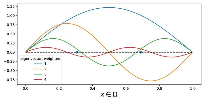
Figure 3. D-optimal measurement locations ($m=5$ measurements) and weighted eigenvectors for inversion of the initial condition of the 1D heat equation. Measurement locations and weighted eigenvectors are plotted over the computational domain $\Omega=[0,1]$ (x-axis). Measurement clusterization occurs approximately at $0.31$ and $0.69$. These two locations are a compromise between zeros of eigenvectors a D-optimal design aims to ignore (third and up) and staying far from a zero of the first and second eigenvectors. Allocating $m=5$ measurements into two locations results in clusterization, according to the pigeonhole principle.

According to Theorem 1, D-optimal designs aim to capture a small subset of eigenvectors of the prior covariance, specifically the $k$ eigenvectors with the highest prior variance. Our model naturally achieves this objective by not measuring eigenvectors $k+1$ and above, as proven in Theorem 1. Translating this understanding to spatial problems, we anticipate that a D-optimal design would favor measurement locations where eigenvectors $k+1$ and above are either close to zero in value or possess small eigenvalues in the prior spectrum, for some $k>0$. To illustrate this preference, Figure 3 depicts the scenario using the 1D heat equation with homogeneous Dirichlet boundary conditions (details in the supplementary material). The plot showcases four eigenvectors, scaled according to their prior standard deviations. Since eigenvectors beyond the fourth have insignificant prior eigenvalues, we exclude them from consideration. Notably, we observe that measurements are clustered near the zeros of the third and fourth eigenvectors, so we conclude that $k=2$. Clusterization arises because there are only two locations where the third and fourth eigenvectors approach zero, while the first and second eigenvectors exhibit significantly non-zero values. Consequently, when we allocate four measurements to these two locations, they naturally cluster together, aligning with the pigeonhole principle.

7. Acknowledgements

This study is a result of research I started during my PhD studies under the instruction of Prof. Georg Stadler at the Courant Institute of Mathematical Sciences. I would like to thank him for his great mentorship, attention to details and kindness. I would also like to thank Christian Remling, who helped me find a proof for Lemma 3 in Mathoverflow.

This research was supported in part by an appointment with the National Science Foundation (NSF) Mathematical Sciences Graduate Internship (MSGI) Program sponsored by the NSF Division of Mathematical Sciences. This program is administered by the Oak Ridge Institute for Science and Education (ORISE) through an interagency agreement between the U.S. Department of Energy (DOE) and NSF. ORISE is managed for DOE by ORAU. All opinions expressed in this paper are the author’s and do not necessarily reflect the policies and views of NSF, ORAU/ORISE, or DOE. This work was also supported by The Raymond and Beverly Sackler Post-Doctoral Scholarship.

References

[1]
Alen Alexanderian, Philip J. Gloor, and Omar Ghattas, On Bayesian A-
and D-optimal experimental designs in infinite dimensions, Bayesian
Analysis 11 (2016), no. 3, 671 – 695, Publisher: International
Society for Bayesian Analysis.
[2]
Alen Alexanderian, Noemi Petra, Georg Stadler, and Omar Ghattas,
A-optimal design of experiments for infinite-dimensional bayesian
linear inverse problems with regularized l0-Sparsification, SIAM Journal
on Scientific Computing 36 (2014), no. 5, A2122–A2148.
[3]
by same author, A fast and scalable method for A-optimal design of experiments
for infinite-dimensional bayesian nonlinear inverse problems, SIAM Journal
on Scientific Computing 38 (2016), no. 1, A243–A272.
[4]
Alen Alexanderian, Noemi Petra, Georg Stadler, and Isaac Sunseri, Optimal
design of large-scale Bayesian linear inverse problems under reducible
model uncertainty: Good to know what you don’t know, SIAM/ASA Journal on
Uncertainty Quantification 9 (2021), no. 1, 163–184, Publisher:
SIAM.
[5]
Alen Alexanderian and Arvind K Saibaba, Efficient D-optimal design of
experiments for infinite-dimensional Bayesian linear inverse problems,
SIAM Journal on Scientific Computing 40 (2018), no. 5, A2956–A2985,
Publisher: SIAM.
[6]
Ahmed Attia and Emil Constantinescu, Optimal Experimental Design for
Inverse Problems in the Presence of Observation Correlations, SIAM
Journal on Scientific Computing 44 (2022), no. 4, A2808–A2842,
Publisher: Society for Industrial and Applied Mathematics.
[7]
Ahmed Attia, Sven Leyffer, and Todd S Munson, Stochastic learning
approach for binary optimization: Application to Bayesian optimal design
of experiments, SIAM Journal on Scientific Computing 44 (2022),
no. 2, B395–B427, Publisher: SIAM.
[8]
Michael Brin and Garrett Stuck, Introduction to dynamical systems,
Cambridge university press, 2002.
[9]
Kathryn Chaloner and Isabella Verdinelli, Bayesian experimental design:
A review, Statistical Science 10 (1995), no. 3, 273–304,
Publisher: JSTOR.
[10]
Barry A. Cipra, An Introduction to the Ising Model, The American
Mathematical Monthly 94 (1987), no. 10, 937–959, Publisher: Taylor
& Francis.
[11]
Thomas M Cover and Joy A Thomas, Elements of information theory, John
Wiley & Sons, 1999.
[12]
Nada Cvetković, Han Cheng Lie, Harshit Bansal, and Karen Veroy-Grepl,
Choosing observation operators to mitigate model error in Bayesian
inverse problems, arXiv preprint arXiv:2301.04863 (2023).
[13]
Valerii V. Fedorov, Design of spatial experiments: Model fitting and
prediction, Tech. Report TM-13152, Oak Ridge National Lab, Oak Ridge,
Tennessee, March 1996.
[14]
Valerii V. Fedorov and Peter Hackl, Model-Oriented Design of
Experiments, Lecture Notes in Statistics, vol. 125, Springer, New
York, NY, 1997.
[15]
E Haber, L Horesh, and L Tenorio, Numerical methods for experimental
design of large-scale linear ill-posed inverse problems, Inverse Problems
24 (2008), no. 5, 055012.
[16]
Lior Horesh, Eldad Haber, and Luis Tenorio, Optimal experimental design
for the large-scale nonlinear ill-posed problem of impedance imaging,
Large-Scale inverse problems and quantification of uncertainty, John
Wiley & Sons, Ltd, 2010, pp. 273–290.
[17]
Jari P. Kaipio and Erkki Somersalo, Statistical and Computational
Inverse Problems, Applied Mathematical Sciences, vol. 160, Springer,
New York, NY, 2005 (en).
[18]
Mehran Kardar, Statistical physics of particles, Cambridge University
Press, Cambridge, 2007.
[19]
Karina Koval, Alen Alexanderian, and Georg Stadler, Optimal experimental
design under irreducible uncertainty for linear inverse problems governed by
PDEs, Inverse Problems (2020), Publisher: IOP Publishing.
[20]
Peter D Lax, Linear algebra and its applications, vol. 78, John Wiley &
Sons, 2007.
[21]
John David Logan, A first course in differential equations, Springer,
2006.
[22]
Ben Marson, Raya Horesh, Lior Horesh, and DS Holder, A new protocol for
the rapid generation of accurate anatomically realistic finite element meshes
of the head from T1 MRI scans, Proc. of IX int. Conf. on electrical
impedance tomography (hanover, NH, USA), 2008, pp. 44–7.
[23]
Ira Neitzel, Konstantin Pieper, Boris Vexler, and Daniel Walter, A sparse
control approach to optimal sensor placement in PDE-constrained parameter
estimation problems, Numerische Mathematik 143 (2019), no. 4,
943–984, Publisher: Springer.
[24]
Joakim Nyberg, Richard Höglund, Martin Bergstrand, Mats O. Karlsson, and
Andrew C. Hooker, Serial correlation in optimal design for nonlinear
mixed effects models, Journal of Pharmacokinetics and Pharmacodynamics
39 (2012), no. 3, 239–249.
[25]
Andrew M Stuart, Inverse problems: a bayesian perspective, Acta numerica
19 (2010), 451–559, Publisher: Cambridge University Press.
[26]
Albert Tarantola, Inverse Problem Theory and Methods for Model
Parameter Estimation, Other Titles in Applied Mathematics, Society
for Industrial and Applied Mathematics, January 2005.
[27]
Dariusz Ucinski, Optimal measurement methods for distributed parameter
system identification, CRC Press, Boca Raton, 2005.
[28]
Curtis R. Vogel, Computational methods for inverse problems, Society for
Industrial and Applied Mathematics, 2002.