Deep Dynamic Factor Models

Abstract

A novel deep neural network framework – that we refer to as Deep Dynamic Factor Model (D²FM) –, is able to encode the information available, from hundreds of macroeconomic and financial time-series into a handful of unobserved latent states. While similar in spirit to traditional dynamic factor models (DFMs), differently from those, this new class of models allows for nonlinearities between factors and observables due to the autoencoder neural network structure. However, by design, the latent states of the model can still be interpreted as in a standard factor model. Both in a fully real-time out-of-sample nowcasting and forecasting exercise with US data and in a Monte Carlo experiment, the D²FM improves over the performances of a state-of-the-art DFM.

Keywords: Machine Learning, Deep Learning, Autoencoders, Real-Time data, Time-Series, Forecasting, Nowcasting, Latent Component Models, Factor Models.

JEL classification: C22, C52, C53, C55.

1 Introduction

An overarching idea in macroeconomics, already shaping the work of Burns and Mitchell (1946), is that a few common forces can explain the joint dynamics of many macroeconomics variables. This stylised view of the economic data generating process has long informed the effort of economic modelling – for example, in the Real Business Cycle (RBC) and Dynamic Stochastic General Equilibrium (DSGE) literature – and is one of the very few robust facts in empirical macroeconomics, motivating the use of factor models (see for example Stock and Watson, 2016).

In macroeconometrics, factor models were firstly introduced by Geweke (1977) and Sargent and Sims (1977) and are a very early instance of ‘big data’ in macroeconomics. Dynamic Factor Models (DFMs) deal with a large cross-section of data (‘large N problem’) by applying a linear dynamic latent state framework to the analysis of economic time-series. The underlying assumption of these models is that there is a small number of pervasive unobserved common factors that stir the economy and inform the comovements of hundreds of economic variables. Economic times series are also possibly affected by variable-specific (idiosyncratic) disturbances. These idiosyncratic disturbances can be due to either measurement error or variable-specific disturbances. Dynamic factor models are workhorse models in macroeconometrics and a large body of empirical evidence has found that, in many applications, a small number of factors – as many as two – can capture a dominant share of the variance of all the key macroeconomic and financial variables.

Factor models are robust and flexible models, also able to accommodate for missing observations, jagged patterns of data and mixed frequencies. However, two of their important limitations are (i) the almost always assumed linear structure, and (ii) the limited scalability of these models due to the computational challenges that are encountered when estimating factors models with more than a few dozens of variables.

This paper introduces a generalisation of factor models in a deep learning framework – which we label Deep Dynamic Factor Models (D²FMs) – that deals effectively with these challenges, while maintaining the same degree of flexibility and of interpretability of a standard DFM. Indeed, our deep learning model can ‘encode’ the information about the state of the economy, as available in real-time, from hundreds of macroeconomic and financial variables at mixed frequency and with ‘jagged edges’, into a handful of unobserved latent states. While similar in spirit to traditional dynamic factor models, differently from those, our model allows for non-linearities both in the encoding – from variables to factors – and in the decoding map – back to the variables from the factors. We also discuss how to generalise it further to nonlinear factor dynamics.

The backbone of our modelling approach is provided by a dynamic autoencoder structure capturing the common information across variables, and whose parameters are estimated via gradient-based backpropagation. An autoencoder is a type of unsupervised learner that maps a number of variables (‘input layer’) into themselves (‘output layer’) by first ‘encoding’ the variables’ common information into a lower dimensional ‘code’ (viz. non-linear factors), and then ‘decoding’ it. Autoencoders are formed by a series of internal (hidden) layers each formed by a number of nodes (neurons). The encoding happens in the first half of the model, and it is the results of a series of non-linear transformations of linear combinations of inputs coming from the previous layer to the current one. Each neuron in each layer operates one of these transformations. The sequence of layers provides ‘depth’ to the neural net, while the number of neurons per layer provides ‘width’. Autoencoders can be thought of as a nonlinear generalisation of principal component analysis (see Hinton and Salakhutdinov, 2006), which are able to transform very high-dimensional data into low-dimensional factors without having to assume a linear factor structure.

The central methodological contribution of our paper is to show how to embed autoencoders in a dynamic nonlinear factor model structure with idiosyncratic components to tackle macroeconomic problems, thus providing generalisation to linear factor models. The equivalence between maximum likelihood estimation and minimisation of mean squared error together with the Universal Approximation Theorem (Cybenko, 1989, Hornik et al., 1989, 1990) allow to reinterpret the D²FMs and the procedure adopted in estimating them as an efficient computational method to approximate the maximum likelihood estimates of a general nonlinear factor models. A second contribution of this paper is to show how to incorporate in this framework general patterns of missing data, jagged edges and mixed frequencies, by extending gradient-based backpropagation methods for autoencoders.

Our methodology is computationally efficient and provides large gains in terms of computational speed when compared to maximum likelihood methods for DFMs. At the best of our knowledge, this paper is the first to adopt an autoencoder structure in a dynamic model with both factor dynamics and dynamic idiosyncratic components, in a state-space framework for real-time high dimensional mixed frequencies time-series data with arbitrary patterns of missing observations.

The proposed D²FM framework is very general and can be, in principle, applied to many different problems both in forecasting and in structural analysis, as done with DFMs. Indeed, the model is designed to be in spirit as close as possible to DFMs.

We test the performances of the D²FM both in a controlled environment through Monte Carlo experiments, and empirically on US data in a forecasting/nowcasting exercise in the spirit of Giannone et al. (2008). The Monte Carlo experiments show that the D²FM largely outperforms the state-of-the-art DFM when the true data generating process is nonlinear, and offers similar performances in the linear case.

In the empirical application, we employ the D²FM to encode a full real-time version of the McCracken and Ng (2016)’s FRED-MD ‘big data’ dataset for the US. The specification of the model and its hyperparameters are not fixed ex-ante but are instead selected in an intensive cross-validation exercise. The model is then evaluated in real-time by comparing its forecasting, nowcasting and backcasting performances against two benchmarks: (i) a univariate AR(1) model; and (ii) a state-of-the-art DFM estimated using a quasi maximum likelihood and an Expectation-Maximisation algorithm (see Giannone et al., 2008 and Banbura and Modugno, 2014). The D²FM outperforms the two benchmarks, in forecasting and in nowcasting, with gains of up to around a 14% improvement when measured in terms of the root mean square forecast errors (RMSFE).

The paper is organised as follows. The remainder of this section discusses the related literature. Section 2 provides some background and the core intuition guiding our methodology: the idea that autoencoders can be seen as static generalisations of PCA, and hence that dynamic versions of these models should be seen as nonlinear generalisations of linear dynamic factor models. Section 3 presents the methodology proposed and discuss its estimation. Section 4 illustrates the Monte Carlo experiments. In section 5 we discuss how to deal with the specificities of economic data. Section 6 describes the empirical application which has the aim to track in real-time the US GDP, using real-time data. Section 7 summarises the main results of the paper and sketches some possible future path of research. Additional technical details and a data description are provided in the Appendix.

Related Literature This work connects three distinct areas of research: the econometric literature focused on dynamic factor model estimation, research on non-linearity in empirical macro models, and deep learning research on autoencoders and latent factor models for analysing time series data.

The key problem in the factor model literature is that, due to the latency of the factors, maximum likelihood estimators cannot be derived explicitly. Geweke (1977) and Sargent and Sims (1977) proposed optimised algorithms for small models in the frequency domain, while Engle and Watson (1981) and Stock and Watson (1989) offered solutions in the time domain. The common drawback of all these proposed methods is that, in general, the maximum likelihood approach is unfeasible for datasets where the cross-section size is large. To solve this problem in Forni and Reichlin (1998), Stock and Watson (2002a) and Giannone et al. (2008) have proposed non-parametric methods based on the principal component analysis to estimate the latent components with large cross-section data. The intuition driving this literature and its applications to macroeconomic problems inform our approach, which can be viewed as providing both a generalisation of standard dynamic factor models, and an efficient numerical approach for handling big data.

Our work also connects to the econometric literature that has explored the extent of nonlinearities in macroeconomic data and proposed univariate and multivariate nonlinear time-series models (see Kock et al., 2011, for a comprehensive literature review). An important part of this literature has estimated dynamic latent models with nonlinearities, which are explicitly modelled through structural breaks, Markov switching regression or threshold regression (see Barnett et al., 2016, Camacho et al., 2012, Marcellino and Schumacher, 2010, Korobilis, 2006 and Nakajima and West, 2013). In this literature, the approach of Bai and Ng (2008) is the closest in spirit to ours and an important early effort at including nonlinearities in factor models. In that paper, either principal components of nonlinear transformation of the data are estimated or nonlinear transformation of the factors are added to a linear factor model. Our methodology is more general. In fact, differently from the procedure of Bai and Ng (2008) our D²FMs needn’t to assume a specific form of nonlinearity either in the encoding or in the decoding map.

Finally, we connect with the strand of the deep learning literature that has explored different approaches to introduce dynamics in autoencoders. The early work of Gregor et al. (2014) proposed the Deep AutoRegressive networks (DARN) in which hidden layers are equipped with autoregressive connections, allowing for dynamics in an autoencoder setting. Successively, Temporal Difference Variation Autoencoders (TD-VAEs) were introduced by Gregor et al. (2019) to model dynamics in autoencoders via long short-term memory networks (LSTM) connections between belief distributions at two distant time steps. A different line of research in this literature has used Deep Learning for State Space models. For example, Krishnan et al. (2017) adopt MLPs to estimate the mean and covariance matrix of a state space with Gaussian transition dynamics. In Fraccaro et al. (2017) a Kalman Variational Autoencoder (K-VAE) is introduced to estimate (locally) linear Gaussian state space models (LGSSM) by disentangling the observations and the latent dynamics. Closer to our approach are the Deep State Space Models (DSSM) of Rangapuram et al. (2018) that directly estimate all the state space parameters using a Recurrent Neural Network (RNN) structure that, given the input features, provides both the latent states and all the time-varying parameters of the state space model. This modelling approach can handle both the presence of noise and missing data. While using deep learning techniques to capture salient features of the data generating process, we tackle those two issues differently. For the former, we apply a denoising approach. For the latter, selection matrices are used to mask missing data when computing the objective to be optimised, while the generative spirit of our model allows to do sampling conditional on the data to fill missing inputs. Importantly, in all the aforementioned approaches, variable specific idiosyncratic components and mixed frequencies are not taken into consideration. We propose a framework able to deal with those two additional data issues. Specifically, we include restriction matrices to aggregate the high frequency latent states to the low frequency as in Mariano and Murasawa (2003) to deal with mixed-frequency, and we design a sequential and iterative (alternated) optimisation scheme between common factors and idiosyncratic components based on a Markov Chain Monte Carlo algorithm.

More generally, deep learning methods have seen early applications in Finance and Economics. In Finance, they have been employed to predict asset prices, stock returns or commodity prices (see Sezer et al., 2019, for an extensive literature review). Closer to our approach, a few recent works have applied neural net to macroeconomic questions. Cook and Hall (2017) employed a number of neural network architectures, including also autoencoder, to forecast the US unemployment rate. Loermann and Maas (2019) proposed a neural net model to predict the US GDP. Holopainen and Sarlin (2017) proposed an horse race among different machine learning methods and showed that such models are able to outperform conventional statistical approaches in predicting crisis periods. Finally, Heaton et al. (2016), Gu et al. (2018, 2019) employ rich datasets incorporating both stock data and macroeconomic aggregates to predict stock returns.

2 Autoencoders and Factor Models

Dynamic factor models for econometric times series are multivariate probabilistic models in which a vector of stochastic disturbances are transmitted via linear dynamic equations to the observed variables. They assume that a small number of stochastic unobserved common factors informs the comovements of hundreds of economic variables. In doing so, they combine two core ideas of macroeconomics: the Frisch-Slutsky paradigm that assumes the economic variables to be generated by the stochastic components (the economic shocks) via usually linear dynamic difference equations; and the idea that has guided macro since Burns and Mitchell (1946) that a few common disturbances explain most of the dynamics of all the macroeconomics variables, with a residual share due to idiosyncratic components. DFMs are similar in intuition to principal component analysis (PCA) but assume stochastic and dynamic structure that allows their application to econometric time series.

Autoencoders (AE) are neural networks trained to map a set of variables into themselves, by first coding the input into a lower dimensional (or undercomplete) representation) and then decoding it back into itself. The lower dimensional representation forces the autoencoder to capture the most salient features of the data. In constructing a nonlinear reflexive map that links the inputs back to itself via a lower dimensional space, autoencoders can be thought of as a nonlinear generalisation of PCA.

In this section, we explore the deep connection between factor models and autoencoders to show that a dynamic formulation of autoencoders can be thought of as a nonlinear generalisations of dynamic factor models, in the same way in which standard autoencoders can be seen as generalisations of principal component analysis.

2.1 Latent Factor Models

Let us first introduce a general formulation of latent factor models with idiosyncratic components. We define $\boldsymbol{y}_{t}=(y_{t,1},...,y_{t,n})$ as the vector collecting the $n$ variables of interest at time $t$, usually assumed to be the realisation of a vector stochastic process. A very general latent factor model can be written as

$$\boldsymbol{y}_{t}=F(\boldsymbol{f}_{t})+\boldsymbol{\varepsilon}_{t}=\widetilde{\boldsymbol{y}}_{t}+\boldsymbol{\varepsilon}_{t}\ ,$$ (1)

where $\boldsymbol{f}_{t}$ is an $r\times 1$ (for $r=dim(\boldsymbol{f})<<n=dim(\boldsymbol{y})$) vector of latent common stochastic components – i.e. the factors –, $\boldsymbol{\varepsilon}_{t}$ are idiosyncratic and unobserved stochastic error terms, and $F(\cdot)$ is a generic function mapping the unobserved factors into the observed variable. Usual assumptions are that $\boldsymbol{f}_{t}$ and $\boldsymbol{\varepsilon}_{t}$ are independent, with zero mean and finite variance (the variance of $\boldsymbol{f}_{t}$ is often assumed to be a diagonal matrix). For later reference, we indicate as $\widetilde{\boldsymbol{y}}_{t}$ the component of $\boldsymbol{y}_{t}$ that relates to the common factors. By assuming also a linear function $F(\cdot)$, the model reduces to the standard linear factor model

$$\boldsymbol{y}_{t}=\boldsymbol{\Lambda}\boldsymbol{f}_{t}+\boldsymbol{\varepsilon}_{t}$$ (2)

However, in general, $F(\cdot)$ needn’t be linear and we can express the factor component of the model as

$$\widetilde{\boldsymbol{y}}_{t}=F(G(\boldsymbol{y}_{t}))=(F\circ G)(\boldsymbol{y}_{t})=(F\circ G)(\widetilde{\boldsymbol{y}}_{t}+\boldsymbol{\varepsilon}_{t}),$$ (3)

where $G(\cdot)$ is the function mapping the observables into the ‘code’ $\boldsymbol{f}_{t}$ (encoding function), and $F(\cdot)$ is the function mapping the factors back into $\boldsymbol{y}_{t}$ (decoding function). In this form, the connection between factor models and autoencoders is more evident. In fact, the map in Equation (3) can be seen as a very general autoencoder. Linear factor models can be seen as a special case of factor models assuming both a linear encoding and a linear decoding function. It is worth observing that the model in Equations (1) and (3), without specifying dynamic equations for the stochastic components, can be seen as purely static model.

2.2 Autoencoders

Autoencoders belong to the deep neural net family of models and have been introduced for applications involving dimensionality reduction (LeCun, 1987, Bourlard and Kamp, 1988, Hinton and Zemel, 1994, Hinton and Salakhutdinov, 2006). Autoencoders solve the parametric problem of finding a mapping (or ‘learning a representation’ in the DNN jargon) of the form $\widetilde{\boldsymbol{y}}_{t}=F(G(\boldsymbol{y}_{t}))$ under the constraint of minimising a loss function of choice

$$\mathcal{L}(\boldsymbol{y}_{t},\widetilde{\boldsymbol{y}}_{t};\boldsymbol{\theta})=\mathcal{L}(\boldsymbol{y}_{t},F(G(\boldsymbol{y}_{t})))\ ,$$ (4)

where $\mathcal{L}(\cdot)$ is the loss function and $\boldsymbol{\theta}$ is the vector collecting all the parameters in $G(\cdot)$ and $F(\cdot)$.

The Principal Components Analysis (PCA) can be seen as the autoencoder minimising the square loss function

$$\mathcal{L}(\boldsymbol{y}_{t},\widetilde{\boldsymbol{y}}_{t};\boldsymbol{\theta})=||\boldsymbol{y}_{t}-\widetilde{\boldsymbol{y}}_{t}||^{2},$$ (5)

and assuming both a linear coding and a linear decoding function, i.e. $\boldsymbol{f}_{t}=G(\boldsymbol{y}_{t})=W^{\prime}\boldsymbol{y}_{t}$ and $\widetilde{\boldsymbol{y}}_{t}=F(\boldsymbol{f}_{t})=\boldsymbol{\Lambda}\boldsymbol{f}_{t}$. Figure 1 provides a neural net representation of PCA.

Figure 1: Principal component analysis (PCA) as an autoencoder.

In principle, $G(\cdot)$ and $F(\cdot)$ can be any nonlinear function and hence finding the correct functional form capturing a data generating process of interest can be a daunting problem. Autoencoders provide a practical implementation of this problem by expressing the composition of two functions as a chain of two multilayer perceptrons (MLPs): the first chain operates the coding, while the second produces the decoded output (see a graphical representation of a symmetric autoencoder in Figure 2). A multilayer perceptron is a type of feedforward artificial neural network composed of a number of ‘hidden’ layers each formed by a number of ‘nodes’ (or ‘neurons’). Each neuron in each layer receives some inputs from the neurons in the previous layer and outputs to the next layer an activation output, $h_{m_{l}}^{l}$. The activation function (or ‘link function’) of each neuron is a nonlinear function parametrised as

$$h_{m_{l}}^{l}=g_{m_{l}}^{l}(\boldsymbol{W}_{m_{l}}^{l}\boldsymbol{h}^{l-1}+b_{m_{l}}^{l})\ ,$$ (6)

where $l$ is the layer (for $l=1,\dots,L$), $m_{l}$ is the node, and $\boldsymbol{\theta}_{m_{l}}^{l}\equiv\{\boldsymbol{W}_{m_{l}}^{l},b_{m_{l}}^{l}\}$ are the parameters of the activation function to be determined, in the form of, respectively, a set of weights and a constant (also called bias). If $l=1$ then, $\boldsymbol{h}_{l-1}=\boldsymbol{h}_{0}=\boldsymbol{y}_{t}$ that is the input data vector. Common choices for the activation function $g_{m_{l}}^{l}(\cdot)$ are the sigmoid, the hyperbolic tangent (tanh), softplus, and the rectified linear unit (ReLu) functions. Hence, in other words, the neuron in each upper layer is the product of an element wise (usually monotone) transformation applied on an affine mapping of the neurons in the lower layer.

Figure 2: A symmetric autoencoder with six observables and three neurons in the code layer (biases are not included in the graph). The first two hidden layers operate the encoding, while the last two hidden layers decode into the output.

We can define as $\boldsymbol{g_{l}}(\cdot)$ the vector containing all the activation functions of a layer $\{g_{1}^{l}(\cdot)\dots g_{M}^{l}(\cdot)\}^{\prime}$ for all the nodes $1,\dots M$. Hence the first MLP will be given by the composition of the activation functions of each node in each layer of the encoding feedforward network, i.e.

$$\boldsymbol{f}_{t}=G(\boldsymbol{y}_{t})={\boldsymbol{g_{L}}}(\boldsymbol{g_{L-1}}(\dots({\boldsymbol{g_{1}}}(\boldsymbol{y}_{t}))))\ .$$ (7)

In a similar way it is usually also defined the MLP operating as decoding network, i.e. as a sequence of layer each containing neurons operating as activation functions over a weighted sum of the inputs plus a constant, i.e.

$$\widetilde{\boldsymbol{y}}_{t}=F(\boldsymbol{y}_{t})=\boldsymbol{\tilde{g}_{L^{\prime}}}(\boldsymbol{\tilde{g}_{L^{\prime}-1}}(\dots({\boldsymbol{\tilde{g}_{1}}}(\boldsymbol{f}_{t}))))\ ,$$ (8)

where $\tilde{g}_{L^{\prime}}$ is the vector of link functions, and $L^{\prime}$ is the number of hidden layers in the decoding network.

While the functional form adopted for the activation functions may seem arbitrary, yet a network with such a structure can approximate any nonlinear continuous function. In fact, the Universal Approximation Theorem, a key result in the neural net literature, states that a feed-forward network even with a single hidden layer, containing a finite number of neurons, can approximate continuous functions on compact subsets of $\mathbb{R}^{n}$, under mild assumptions on the activation function. However, it does not guarantee that the algorithm adopted to estimate the network can learn the correct parameters (see Cybenko, 1989, Hornik et al., 1989, 1990 and Lu et al., 2017).

The autoencoder is said to be symmetric when the number of hidden layers in the encoding and in the decoding networks are the same (i.e. $L^{\prime}=L$), otherwise asymmetric. Asymmetric autoencoders usually have several layers of encoding but only a single layer of decoding (i.e. $L^{\prime}=1$), hence the decoding network is not a MLP but an SLP (single layer perceptron).

For a given choice of the link functions, the parameter vector of the autoencoder $\boldsymbol{\theta}$ contains the full set of weights and constants (biases) that define the affine transformations operated by each neuron before the link function is applied. These parameters are determined by minimising the loss function $\mathcal{L}(\boldsymbol{y}_{t},\widetilde{\boldsymbol{y}}_{t};\boldsymbol{\theta})=\mathcal{L}(\boldsymbol{y}_{t},F(G(\boldsymbol{y}_{t}));\boldsymbol{\theta})$, via back-propagation (Rumelhart et al., 1986 and LeCun, 1987). One way to estimate autoencoders is by corrupting the inputs with noise injection (see Vincent et al., 2008) during the training process. Those are referred as Denoising Autoencoders. The intuition for this procedure is that, as discussed in Vincent et al. (2008) and Bengio et al. (2013), it forces the model to learn the data distribution and not only the distribution specific of the sample used, thanks to data augmentation. Also, noise injection can be seen as a procedure to improve the robustness of neural networks.

2.3 Dynamics in Factor Models

So far we have discussed the general structure of factor models by abstracting from the dynamics and focusing on the ‘static’ map into lower dimensional factors. Dynamics is usually introduced in DFMs by assuming that both $\boldsymbol{f}_{t}$ and $\boldsymbol{\varepsilon}_{t}$ are generated by linear stochastic vector difference equations. For example, Banbura et al. (2010) and Banbura and Modugno (2014) consider a system specified as

$$\boldsymbol{y}_{t} =\boldsymbol{\Lambda}\boldsymbol{f}_{t}+\boldsymbol{\varepsilon}_{t}\ ,$$ (9)

$$\boldsymbol{f}_{t} =\boldsymbol{B}_{1}\boldsymbol{f}_{t-1}+\dots+\boldsymbol{B}_{p}\boldsymbol{f}_{t-p}+\boldsymbol{u}_{t},\quad\quad\boldsymbol{u}_{t}\overset{iid}{\sim}\mathcal{N}(0,\boldsymbol{U}),$$ (10)

$$\boldsymbol{\varepsilon}_{t} =\boldsymbol{\Phi}_{1}\boldsymbol{\varepsilon}_{t-1}+\dots+\boldsymbol{\Phi}_{d}\boldsymbol{\varepsilon}_{t-d}+\boldsymbol{\epsilon}_{t},\quad\quad\boldsymbol{\epsilon}_{t}\overset{iid}{\sim}\mathcal{N}(0,\boldsymbol{Q}),$$ (11)

where $\boldsymbol{B}_{1},\dots,\boldsymbol{B}_{p}$ are the $r\times r$ matrices of autoregressive coefficients for the factor and $\boldsymbol{\Phi}_{1},\dots,\boldsymbol{\Phi}_{d}$ are the $n\times n$ diagonal matrices of autoregressive coefficients for the idiosyncratic component (i.e. $\boldsymbol{\Phi}_{1}=diag(\phi_{1},\dots,\phi_{n})$). Specifically, Banbura et al. (2010) and Banbura and Modugno (2014) assume a VAR process of order two ($p=2$) for factors, and of order one ($d=1$) for the idiosyncratic component.

Such a structure can be seen, in our framework, as obtained by assuming that:

• Encoding function $G_{\theta_{G}}(\cdot):\boldsymbol{y}\rightarrow\boldsymbol{f}$ is a linear operator;

• Decoding function $F_{\theta_{F}}(\cdot):\boldsymbol{f}\rightarrow\widetilde{\boldsymbol{y}}$ is a linear operator;

• Factor dynamics $\boldsymbol{f}_{t}$ follows a linear stochastic vector difference equation;

• Idiosyncratic component dynamics $\boldsymbol{\varepsilon}_{t}$ follows a linear stochastic vector difference equation with diagonal matrices of autoregressive coefficients;

• Distributions Error terms from the transition (and emission) equations are assumed to be $i.i.d.$ Gaussian.

Autoencoders provide a practical solution to estimate factor models with a more general structure, potentially relaxing one or all of these assumptions to obtain both nonlinear maps from reduced dimension factors to variables and vice-versa, but also to introduce nonlinear dynamic equations. This approach to the generalisation of dynamic factor models, is what we call Deep Dynamic Factor Models (D²FMs). In the next section, we show how to construct and estimate an autoencoder that relaxes assumptions A.1 and A.2, while maintaining the others.

2.4 Estimation and Conditional Likelihood

In principle the parameters of a parametric factor model of the form $\boldsymbol{y}_{t}=F(\boldsymbol{f}_{t})+\boldsymbol{\varepsilon}_{t}$ would be estimated via maximum likelihood,

$$\boldsymbol{\widehat{\theta}}=\operatorname*{argmax}_{\boldsymbol{\theta}}p_{model}(\boldsymbol{Y};\boldsymbol{\theta})\ ,$$ (12)

where by $\boldsymbol{Y}$ is the full sample of observation, and $p_{model}(\cdot;\cdot)$ is the conditional probability density function of the model.

However, a direct maximum likelihood is rarely feasible, even for linear models, and iterative methods to find maximum likelihood or maximum a posteriori (MAP) estimates of the parameters of the model are preferred. In fact, maximum likelihood estimators of the parameters $\boldsymbol{\theta}=(\boldsymbol{\Lambda},\boldsymbol{B}(L),\boldsymbol{U},\boldsymbol{\Phi}(L),\boldsymbol{Q})$ are in general not available in closed form and a direct numerical maximisation can be too demanding when $n$ is large. Indeed, a proposed solution in the linear factor model literature is to adopt the Expectation Maximisation (EM) algorithm, a maximum a posteriori method, and to initialise the common factors $\boldsymbol{f}_{t}$ with PCA on the observables. The updates of the latent components are performed using the Kalman filter and smoother.

A similar approach can be adopted from a ‘deep’ point of view on factor models by employing the methodologies developed in the deep learning literature, without losing the dynamic model interpretation. As we discuss in the next section, the model parameters of a D²FM can be estimated via Monte Carlo gradient methods, instead of using the EM algorithm. This has computational advantages – the methods are fast and reliable – even when the dataset is big. At the same time, estimation results can be thought of as approximating a maximum a posteriori method.

It is well know, in the linear case, that if the innovation $\boldsymbol{\varepsilon}_{t}$ are assumed to be independent (or uncorrelated) of $\boldsymbol{f}_{t}$ and normally distributed, than the maximisation of the likelihood with respect to the parameters of the model yields the same estimate for the parameters as does minimising the mean squared error.

Importantly, this equivalence between maximum likelihood estimation and minimisation of mean squared error holds regardless of the function used to predict the mean of the Gaussian distributed variable $\boldsymbol{y}_{t}$ (see Goodfellow et al., 2016). This result allows for an interpretation of estimation results from autoencoders with mean squared error from a Bayesian perspective, using standard likelihood methods, or from a frequentist one as the (approximated) mean estimator of a Gaussian distributed process.

Furthermore, the equivalence between maximum likelihood estimation and minimisation of mean squared error together with the Universal Approximation Theorem allow to reinterpret the autoencoders and the procedure adopted in estimating them as an efficient computational method to approximate the maximum likelihood estimates of nonlinear factor models. These are dynamic models that are defined by a conditionally Gaussian distribution centred around a mean provided by a nonlinear but continuous function of the inputs. In the next section, we provide an algorithm that implements Deep Dynamic Factor Models.

3 D²FM Estimation

In its general form, the D²FM can be written as

$$\boldsymbol{f}_{t} =G(\boldsymbol{y}_{t})\ ,$$ (13)

$$\boldsymbol{y}_{t} =F(\boldsymbol{f}_{t})+\boldsymbol{\varepsilon}_{t}\ ,$$ (14)

$$\boldsymbol{f}_{t} =\boldsymbol{B}_{1}\boldsymbol{f}_{t-1}+\dots+\boldsymbol{B}_{p}\boldsymbol{f}_{t-p}+\boldsymbol{u}_{t},\quad\quad\boldsymbol{u}_{t}\overset{iid}{\sim}\mathcal{N}(0,\boldsymbol{U}),$$ (15)

$$\boldsymbol{\varepsilon}_{t} =\boldsymbol{\Phi}_{1}\boldsymbol{\varepsilon}_{t-1}+\dots+\boldsymbol{\Phi}_{d}\boldsymbol{\varepsilon}_{t-d}+\boldsymbol{\epsilon}_{t},\quad\quad\boldsymbol{\epsilon}_{t}\overset{iid}{\sim}\mathcal{N}(0,\boldsymbol{Q}),$$ (16)

where the assumptions on the linearity of the dynamic equations are maintained, Equations (15) and (16), while the model allows for a nonlinear map between variables and factors. The estimation of linear factor dynamics separately creates what Stock and Watson (2011) call a ‘state space with static (common) factors’ as opposed to a ‘state space with dynamic (common) factors’.

The D²FM can be implemented using a symmetric autoencoder architecture with a MLP capturing the encoding function, Equation (13), and another MLP providing the nonlinear decoding, Equation (14). The assumption of i.i.d. and Gaussian innovations allows for an interpretation of the estimated network as MAP of the likelihood of the model (see Goodfellow et al., 2016).

Importantly, such a model specification encompasses several simplified models, most notably the standard linear DFMs, and hence the estimation algorithm can be specialised to the scope.

3.1 Network Design

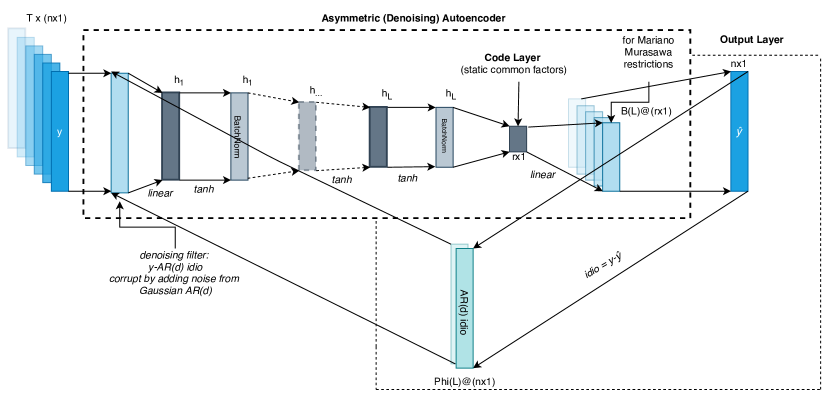
Figure 3: A graph representation of the training process for a the D²FM with an asymmetric structure: nonlinear multilayer encoder and linear single layer decoder.

The core of the model is provided by an autoencoder with a nonlinear multilayer encoder and either a symmetric structure in the decoding, for nonlinear decoding, or an asymmetric structure with a linear single layer decoder. Linear stochastic autoregressive equations are adopted to model the dynamics of factors and idiosyncratic components. Figure 3 shows a diagrammatic representation of the model with a single layer decoder.

The number of hidden layers in the encoding network as well as the number of neurons need not be pre-specified but can be selected via cross-validation. This enables the model to capture different degrees of complexity in the data, which is not know a-priori. With respect to the activation functions, we equip each neuron in the coding layers with a link function in the form of the hyperbolic tangent (tanh) for the real-time macroeconomic dataset, and of the rectified linear unit (ReLU) for the Monte Carlo exercises. In the encoding multilayer perceptron we also include two batch normalisation layers to induce some regularisation, and control over potential covariate shift (see Ioffe and Szegedy, 2015).

In the decoding network, an additional linear layer can be included to introduce constraints needed to account for the mixed frequencies of macroeconomic data. This additional layer does not have any additional parameter, and it only includes aggregation weights to map the high frequency latent states to the low frequency observables.

3.2 Estimation and Online Learning of the D²FM

In our estimation of the D²FM, we propose a two-step procedure to differentiate between on-line (out-of-sample) and off-line (in-sample) learning.

• Step 1 estimate off-line all the parameters of the model;

• Step 2 cast the decoding part in a state-space framework to allow for on-line updates of the latent states given the observables.

Algorithm 1 implements the off-line estimation step (Step 1) of our D²FM, assuming an AR(d) for $p_{idio}(\cdot)$, but possibly a general encoding $G_{\theta_{G}}(\cdot)$ and decoding $F_{\theta_{F}}(\cdot)$ function. The proposed algorithm for estimating D²FM builds on and extends what has been proposed by Bengio et al. (2013) to estimate Generalised Denoising Autoencoders.

Algorithm 1 MCMC for D²FM with stationary AR(d) idiosyncratic components – requires a training set, an encoding structure $G_{\boldsymbol{\theta}_{G}}(\cdot)$ and a decoding one $F_{\boldsymbol{\theta}_{F}}(\cdot)$

1:init: $\boldsymbol{\theta}_{G},\boldsymbol{\theta}_{F},\boldsymbol{\Phi},\Sigma_{\varepsilon},\boldsymbol{\varepsilon}_{t}$

2:repeat

3:$\quad\widetilde{\boldsymbol{y}}_{t}|(\boldsymbol{y}_{t},\hat{\boldsymbol{\varepsilon}}_{t})=\boldsymbol{y}_{t}-\boldsymbol{\Phi}(L)\boldsymbol{\varepsilon}_{t}$

4:    Loop epochs, batches Do

5:      draw $\boldsymbol{\varepsilon}^{(mc)}_{t}\overset{iid}{\sim}\mathcal{N}(0,\Sigma_{\varepsilon})$

6:$\quad\quad\boldsymbol{y}^{(mc)}_{t}=\widetilde{\boldsymbol{y}}_{t}|(\boldsymbol{y}_{t},\hat{\boldsymbol{\varepsilon}}_{t})+\boldsymbol{\varepsilon}^{(mc)}_{t}$

7:$\quad\quad\theta_{G},\theta_{F}$ update by a gradient based step on $\mathcal{\hat{L}}(\boldsymbol{y}_{t},F_{\boldsymbol{\theta}_{F}}(G_{\boldsymbol{\theta}_{G}}(\boldsymbol{y}^{(mc)}_{t})))$

8:    End Loop

9:$\quad\boldsymbol{f}_{t}|\boldsymbol{y}^{(mc)}_{t}=\mathbb{E}_{\boldsymbol{y}^{(mc)}_{t}\sim\boldsymbol{y}_{t},\hat{\boldsymbol{\varepsilon}}_{t}}G_{\boldsymbol{\theta}_{G}}(\boldsymbol{y}^{(mc)}_{t})$

10:$\quad\boldsymbol{\varepsilon}_{t}|\boldsymbol{y}_{t},\boldsymbol{f}_{t}=\boldsymbol{y}_{t}-F_{\boldsymbol{\theta}_{F}}(\boldsymbol{f}_{t}|\boldsymbol{y}^{(mc)}_{t})$

11:$\quad\boldsymbol{\Phi}\leftarrow stationary\;AR(d)\;$ on $\;\boldsymbol{\varepsilon}_{t}$

12:$\quad\Sigma_{\varepsilon}\leftarrow from\;\boldsymbol{\varepsilon}_{t}$

13:until convergence on $\mathcal{\hat{L}}(\boldsymbol{y}_{t},F_{\boldsymbol{\theta}_{F}}(\boldsymbol{f}_{t}|\boldsymbol{y}^{(mc)}_{t}))$ in $L_{1}$ norm

14:return $\Sigma_{\varepsilon},\boldsymbol{\Phi},\boldsymbol{f}_{t},F_{\boldsymbol{\theta}_{F}}$

Let us present the estimation algorithm. Parameters are first initialised. Line 1 performs a filtering of the input data ${\boldsymbol{y}}_{t}$ by using the conditional mean of the AR(d) of the idiosyncratic components. From lines 2 to 6, the Monte Carlo step and the gradient updates over each epoch and batch are carried out, employing the filtered data $\widetilde{\boldsymbol{y}}_{t}$ and injecting Gaussian noise from $\boldsymbol{\varepsilon}_{t}$ in a denoising fashion to obtain the noisy observations $\boldsymbol{y}^{(mc)}_{t}$. In line 7, the latent states $\boldsymbol{f}_{t}$ are extracted from the encoding network via Monte Carlo integration, while from line 8 to 10 the algorithm updates the parameters of the idiosyncratic process $\boldsymbol{\varepsilon}_{t}$, conditional on the factors and the observables. The adoption of an $L_{2}$ (MSE) loss function $\mathcal{\hat{L}}(\boldsymbol{y}_{t},F_{\boldsymbol{\theta}_{F}}(\boldsymbol{f}_{t}|\boldsymbol{y}^{(mc)}_{t}))$ allows for interpretability of the results, as discussed. We specify an estimated loss, as missing data prevents us from deriving the exact loss. Finally, convergence is checked as the $L_{1}$ norm of the distance between the loss function at two iterations. It is worth noting that the loss, $\mathcal{\hat{L}}(\cdot)$ includes only the common components, since under our assumptions at convergence we have the following decomposition of the log-likehood:

$$\begin{split}&\log p_{model}(\boldsymbol{y}_{t}|\boldsymbol{f}_{t}=G_{\theta_{G}}(\boldsymbol{y}^{(mc)}_{t}),\boldsymbol{\varepsilon}_{t}=\hat{\boldsymbol{\varepsilon}}_{t})=\\ &\log p_{decoder}(\boldsymbol{y}_{t}|\boldsymbol{f}_{t}=G_{\theta_{G}}(\boldsymbol{y}^{(mc)}_{t}))+\log p_{idio}(\boldsymbol{y}_{t}|\boldsymbol{\varepsilon}_{t}=\hat{\boldsymbol{\varepsilon}}_{t})\ ,\end{split}$$ (17)

where $\hat{\boldsymbol{\varepsilon}}_{t}$ is the estimated idiosyncratic autoregressive component. In running over epochs and batches (lines 2 to 6), the algorithm injects uncorrelated noise into the data (it is a Denoising Autoencoder). Hence it searches for a maximum a posteriori of the parameters for the modified model with log-likelihood

$$\mathbb{E}_{\boldsymbol{y}_{t}\sim\ p_{data}(\boldsymbol{y}_{t})}\mathbb{E}_{\boldsymbol{y}^{(mc)}_{t}\sim p_{noisy}(\boldsymbol{y}^{(mc)}_{t}|\boldsymbol{y}_{t},\hat{\boldsymbol{\varepsilon}}_{t})}\log\>p_{model}(\boldsymbol{y}_{t}|\boldsymbol{f}_{t}=G_{\theta_{G}}(\boldsymbol{y}^{(mc)}_{t}),\boldsymbol{\varepsilon}_{t}=\hat{\boldsymbol{\varepsilon}}_{t})\ ,$$ (18)

where $p_{noisy}(\boldsymbol{y}^{(mc)}_{t}|\boldsymbol{y}_{t},\hat{\boldsymbol{\varepsilon}}_{t})$ is the corruption distribution, using a Gaussian autoregressive process. The idea behind this procedure is to filter out the foreseeable idiosyncratic part from the input variables, so that only the common component(s) remain(s). Injecting noise from the unconditional idiosyncratic distribution will generate new samples which are not unreasonably far from the old ones. In doing so, we define an appealing and convenient linkage between the corruption process of the denoising approach and the idiosyncratic component distribution ($p_{idio}$).

In Step 2, the output of the algorithm is cast in the state-space of equations (14)-(16). Dynamics of the common factors are estimated via OLS or Maximum Likelihood. State updates can then be carried out via either nonlinear filtering procedures for a nonlinear decoder, or via Kalman filtering in the presence of a linear decoder. This allows for online (i.e., out-of-sample) learning with the flow of data.

3.3 Cross-Validating Hyperparameters

The D²FM described in this section is subject to the selection of a number of critical parameters determining its structure, beyond the coefficients $\boldsymbol{\theta}$. These parameters are commonly known as hyperparameters, being them set before the training starts and usually selected over a grid with respect to some validation loss, which is estimated via a process called cross-validation.

The D²FM has hyperparameters typical of both deep learning and time-series models. In particular, the deep learning hyperparameters can be divided into two categories. The first relates to the neural network structure and includes: the type of layers, the number of hidden layers, the number of neurons per each hidden layer, penalisation coefficients, dropout layers and relative dropout rates (if included), batch normalisation layers and the link function used. The second category relates to the optimisation algorithm used and comprehends: size of the mini-batches, number of epochs, the learning rate and the momentum coefficients of the gradient optimisation method, if present. Standard time-series factor models have few additional hyperparameters which include: the number of latent common states, the number of lags of the input variables, the number of lags of the latent common states and of the idiosyncratic states. These hyperparameters, in the time series literature, are either fixed a-priori or estimated using information criteria instead of grid-search algorithms.

It is important to observe that in time-series we cannot apply the common ‘K-fold’ cross-validation method because usually its technical conditions are not met (see Bergmeir et al., 2018, for details). Therefore, we use a standard out-of-sample approach which consists in splitting the set of observations available up to a certain point in time, $T$, between a training set $[0,T-k*h-1]$, and validation set $[T-k*h,T-(k-1)*h]$, where $h$ determines the length of the set, while $k=K,\dots,1$ with $K\ll\frac{T-1}{h}$. By averaging over the losses computed on the $K$ ‘validation sets’, we get an estimate of the ‘validation loss’. This means that we need to estimate a given model with fixed hyperparameter $K$ times, and this for each possible hyperparameters combination. Therefore, with deterministic search method the computational cost is exponential in the dimensionality of the hyperparameters.

4 Monte Carlo Experiment

In this section, we compare the performances of DFMs and of D²FM in a controlled environment, by simulating artificial time series data with Monte Carlo experiments. In doing so, we first consider the linear data generating processes studied in Doz et al. (2012) and Banbura and Modugno (2014), and then, adopt its nonlinear generalisation proposed by Gu et al. (2019). In particular, we consider data generated the following process:

$$\boldsymbol{y}_{t} =F(\boldsymbol{f}_{t})+\boldsymbol{\varepsilon}_{t}+\boldsymbol{v}_{t}\ ,$$ (19)

$$\boldsymbol{f}_{t} =\boldsymbol{B}_{1}\boldsymbol{f}_{t-1}+\boldsymbol{u}_{t},\quad\quad\boldsymbol{u}_{t}\overset{iid}{\sim}\mathcal{N}(0,\boldsymbol{I}_{r}),$$ (20)

$$\boldsymbol{\varepsilon}_{t} =\boldsymbol{\Phi}_{1}\boldsymbol{\varepsilon}_{t-1}+\boldsymbol{\epsilon}_{t},\quad\quad\boldsymbol{\epsilon}_{t}\overset{iid}{\sim}\mathcal{N}(0,\boldsymbol{Q}),$$ (21)

for $t=1,\dots,T$. As in Gu et al. (2019), we simulate both a linear, and nonlinear factor model, and allow $F(\cdot)$ to take two forms:

$$F(\boldsymbol{f}_{t})=\begin{cases}\boldsymbol{\Lambda}\boldsymbol{f}_{t}&\text{if linear}\\ \boldsymbol{\Lambda}[\boldsymbol{f}_{t},poly(\boldsymbol{f}_{t},2),sgn(\boldsymbol{f}_{t})]^{\prime}&\text{if nonlinear}\end{cases},$$ (22)

where $sgn(\cdot)$ is the sign function ($1$ if positive, $-1$ if negative) and $poly(\cdot,2)$ is a generator of polynomial functions of order $2$. The parameters of the model are set as follows:

$$\boldsymbol{\Lambda}_{ij}\overset{iid}{\sim}\mathcal{N}(0,1),\qquad\ i=1,\dots,n,\qquad\, j=1,\dots,\tilde{r},$$ (23)

$$\tilde{r}=\begin{cases}r&\text{linear}\\ \frac{4r+r(r+1)}{2}&\text{nonlinear}\end{cases},$$ (24)

$$\boldsymbol{B}_{ij,1}=\begin{cases}\rho&\text{if }i=j\\ 0&\text{otherwise}\end{cases}, \qquad\boldsymbol{\Phi}_{ij,1}=\begin{cases}\alpha&\text{if }i=j\\ 0&\text{otherwise}\end{cases},$$ (25)

$$\boldsymbol{Q}_{ij}=\tau^{|i-j|}(1-\alpha^{2})\sqrt{\gamma_{i}\gamma_{j}}, \quad\gamma_{i}=\frac{\beta_{i}}{1-\beta_{i}}\frac{1}{1-\rho^{2}}\sum_{j=1}^{\tilde{r}}\boldsymbol{\Lambda}^{2}_{ij},$$ (26)

$$\beta_{i}\sim U([u,1-u]).$$ (27)

We consider a range of possible specifications of the parameters by setting the number of factors $r=\{1,3\}$, the number of variables $n=\{10,100\}$, autoregressive coefficient of the factors $\rho=\{0.5,0.9\}$, autoregressive coefficient of the idiosyncratic component $\alpha=\{0,0.5\}$, the number of observations $T=\{50,200\}$, and the fraction of missings is in $\{0,0.3\}$.

For each setting, we run 100 Monte Carlo simulations and estimate a DFM, and a four layers D²FM, with a ReLU activation function augmented with three BatchNorm layers. The number of factors is set for both models to the true number of factors (i.e. $r$ when the DGP is linear in the factors and $\tilde{r}$ when it is nonlinear). Starting from the factor layer, hidden neurons increase by a factor of two in each layer up to the input layer.

As in Stock and Watson (2002a), Doz et al. (2012) and Banbura and Modugno (2014), we compare the models based on the trace $R^{2}$ of the regression of the estimated factors on the true ones

$$\frac{Trace(F^{\prime}\hat{F}(\hat{F}^{\prime}\hat{F})^{-1}\hat{F}^{\prime}F)}{Trace(F^{\prime}F)}\ ,$$ (28)

where $\hat{F}=\mathbb{E}_{\boldsymbol{\hat{\theta}}}[F|H_{T}]$ and $H_{T}$ is the history of the data.

In the linear case, differences in performances between the D²FM and the DFM (Table 1) are very small, and indicate a marginal gain for one model or the other, depending on the specific case. This points to the fact that the two framework are generally equivalent when the DGP is linear. In other words, the D²FM can be seen as a computational efficient way to estimate linear factor models, conditional on a linear DGP.

In the nonlinear simulations (Table 2), the D²FM is instead clearly superior. Strikingly, all the differences are statistically significant and the D²FM can explain between $15\%$ and $34\%$ more of the total variance of the simulated common factors. These results validate the ability of the D²FM to better handle several forms of nonlinearities in the DGP, as compared to a standard DFM.

Factors				1
Sample				50			200
$\alpha$	$\rho$	N vars	Missings	D2FM	DFM	Diff.	D2FM	DFM	Diff.
0	0.5	10	0	0.91	0.89	0.025***	0.94	0.94	-0.008***
0	0.5	10	0.3	0.88	0.83	0.045***	0.91	0.91	-0.006***
0	0.5	100	0	0.96	0.95	0.011***	0.99	0.99	-0.001***
0	0.5	100	0.3	0.95	0.93	0.02***	0.99	0.99	0.001
0	0.9	10	0	0.74	0.75	-0.011	0.94	0.95	-0.01***
0	0.9	10	0.3	0.71	0.70	0.001*	0.93	0.94	-0.013***
0	0.9	100	0	0.77	0.74	0.024	0.96	0.96	0.001***
0	0.9	100	0.3	0.76	0.75	0.017***	0.96	0.96	0.002
0.5	0.5	10	0	0.90	0.85	0.043***	0.92	0.92	0.001
0.5	0.5	10	0.3	0.85	0.77	0.086***	0.88	0.89	-0.008
0.5	0.5	100	0	0.96	0.94	0.013***	0.99	0.99	-0.001***
0.5	0.5	100	0.3	0.95	0.94	0.015***	0.98	0.99	-0.001***
0.5	0.9	10	0	0.72	0.72	0.004***	0.93	0.93	0
0.5	0.9	10	0.3	0.71	0.70	0.007***	0.92	0.93	-0.004***
0.5	0.9	100	0	0.77	0.73	0.035**	0.96	0.96	0.001***
0.5	0.9	100	0.3	0.76	0.75	0.018***	0.96	0.96	0.002***
Factors				3
Sample				50			200
$\alpha$	$\rho$	N vars	Missings	D2FM	DFM	Diff.	D2FM	DFM	Diff.
0	0.5	10	0	0.71	0.71	-0.001**	0.76	0.80	-0.039***
0	0.5	10	0.3	0.60	0.58	0.021	0.66	0.71	-0.051***
0	0.5	100	0	0.94	0.91	0.021***	0.97	0.97	-0.002***
0	0.5	100	0.3	0.92	0.91	0.014***	0.96	0.96	0.002
0	0.9	10	0	0.63	0.66	-0.029***	0.82	0.88	-0.06***
0	0.9	10	0.3	0.58	0.64	-0.066***	0.75	0.85	-0.101***
0	0.9	100	0	0.74	0.74	0.003***	0.92	0.92	-0.001***
0	0.9	100	0.3	0.73	0.73	-0.002	0.92	0.92	-0.003***
0.5	0.5	10	0	0.67	0.63	0.044***	0.70	0.69	0.01
0.5	0.5	10	0.3	0.56	0.52	0.035***	0.60	0.61	-0.013***
0.5	0.5	100	0	0.93	0.91	0.021***	0.97	0.97	0
0.5	0.5	100	0.3	0.92	0.88	0.033***	0.96	0.95	0.002
0.5	0.9	10	0	0.60	0.63	-0.031***	0.77	0.85	-0.083***
0.5	0.9	10	0.3	0.55	0.61	-0.063***	0.70	0.82	-0.12***
0.5	0.9	100	0	0.74	0.74	0.001***	0.92	0.92	0
0.5	0.9	100	0.3	0.73	0.72	0.01**	0.92	0.92	-0.002***

Table 1: Linear DGP. Median over 100 Monte Carlo simulations of the Trace of the $R^{2}$ between estimated and true factors. The difference is computed as: $R^{2}_{D^{2}FM}-R^{2}_{DFM}$. Significance level are based on a two sided Wilcoxon signed-rank test: * for $10\%$, ** for $5\%$ and *** for $1\%$.

Factors				1
Sample				50			200
$\alpha$	$\rho$	N vars	Missings	D2FM	DFM	Diff.	D2FM	DFM	Diff.
0	0.5	10	0	0.849	0.63	0.223***	0.88	0.66	0.217***
0	0.5	10	0.3	0.791	0.55	0.245***	0.827	0.61	0.22***
0	0.5	100	0	0.908	0.72	0.187***	0.911	0.76	0.154***
0	0.5	100	0.3	0.906	0.7	0.208***	0.912	0.74	0.17***
0	0.9	10	0	0.93	0.6	0.335***	0.945	0.64	0.302***
0	0.9	10	0.3	0.914	0.59	0.323***	0.94	0.64	0.299***
0	0.9	100	0	0.941	0.61	0.334***	0.96	0.65	0.308***
0	0.9	100	0.3	0.947	0.61	0.336***	0.962	0.66	0.305***
0.5	0.5	10	0	0.862	0.59	0.274***	0.87	0.63	0.241***
0.5	0.5	10	0.3	0.787	0.51	0.276***	0.802	0.58	0.222***
0.5	0.5	100	0	0.913	0.71	0.199***	0.912	0.75	0.161***
0.5	0.5	100	0.3	0.908	0.69	0.216***	0.911	0.74	0.17***
0.5	0.9	10	0	0.932	0.59	0.342***	0.948	0.64	0.308***
0.5	0.9	10	0.3	0.909	0.6	0.314***	0.934	0.64	0.295***
0.5	0.9	100	0	0.929	0.61	0.322***	0.962	0.65	0.31***
0.5	0.9	100	0.3	0.941	0.61	0.332***	0.961	0.66	0.303***
Factors				3
Sample				50			200
$\alpha$	$\rho$	N vars	Missings	D2FM	DFM	Diff.	D2FM	DFM	Diff.
0	0.5	10	0	0.741	0.51	0.228***	0.662	0.44	0.224***
0	0.5	10	0.3	0.653	0.43	0.223***	0.547	0.34	0.203***
0	0.5	100	0	0.927	0.74	0.191***	0.948	0.76	0.184***
0	0.5	100	0.3	0.871	0.68	0.188***	0.924	0.73	0.193***
0	0.9	10	0	0.94	0.61	0.332***	0.926	0.65	0.274***
0	0.9	10	0.3	0.884	0.61	0.279***	0.863	0.64	0.226***
0	0.9	100	0	0.978	0.67	0.309***	0.987	0.73	0.253***
0	0.9	100	0.3	0.974	0.68	0.296***	0.984	0.75	0.232***
0.5	0.5	10	0	0.735	0.51	0.227***	0.638	0.42	0.222***
0.5	0.5	10	0.3	0.646	0.43	0.213***	0.526	0.34	0.189***
0.5	0.5	100	0	0.907	0.72	0.189***	0.936	0.75	0.188***
0.5	0.5	100	0.3	0.85	0.66	0.191***	0.91	0.71	0.197***
0.5	0.9	10	0	0.942	0.61	0.332***	0.922	0.64	0.278***
0.5	0.9	10	0.3	0.884	0.62	0.267***	0.857	0.64	0.222***
0.5	0.9	100	0	0.978	0.67	0.31***	0.985	0.73	0.253***
0.5	0.9	100	0.3	0.974	0.68	0.298***	0.982	0.74	0.238***

Table 2: Nonlinear DGP. Median over 100 Monte Carlo simulations of the Trace of the $R^{2}$ between estimated and true factors. The difference is computed as: $R^{2}_{D^{2}FM}-R^{2}_{DFM}$. Significance level are based on a two sided Wilcoxon signed-rank test: * for $10\%$, ** for $5\%$ and *** for $1\%$.

An additional key advantage of the D²FM are the superior performances from the point of view of its computational time. In Table 3 we compare the computational time required to estimate a DFM versus a D²FM. The table shows clear computational advantages in favour of the gradient based Monte Carlo approach of the D²FM as compared to the OLS EM approach of the DFM, when the dataset features many variables (starting with $150$ observable variables, in the case of our experiments).

	Number of observations
Number of Variables	150	300
50	0.48	0.22
150	1.29	1.15
300	2.90	2.07

Table 3: Second order polynomial DGP with 3 factors. The table shows ratio of the DFM to the D²FM elapsed times taken to build and fit the model. Each elapsed time is computed as an average over 20 runs. Both models are estimated using an Intel Core i7-8750H CPU @ 2.20GHz. We use tensorflow to estimate the D²FM in eager mode as opposed to graph mode to make the performance comparable.

5 A Deep Dynamic Factor Model for Macro Data

To apply our model to macroeconomic data in a nowcasting and forecasting exercise, we need to introduce a version of the D²FM able to track and forecast developments in economic variables in real-time. We modify the model to efficiently encode mixed-frequency data with ragged edges. In fact, economic data in real time are generally not available at the same frequency – be it weekly, monthly or quarterly –, and missing data are a feature of real-time macroeconomic datasets, due to the non-synchronous and staggered data releases of new datapoints from statistical offices.

As in the previous section, we specify a linear mapping between the factors and the variables (see Figure 3), i.e.

$$\boldsymbol{y}_{t} =\boldsymbol{\Lambda}\boldsymbol{f}_{t}+\boldsymbol{\varepsilon}_{t}\ .$$ (14^′)

In this form, the model can be seen as a very flexible generalisation of the approach of Bai and Ng (2008) that propose to extract factors from variables as well as their squared values and their crossproducts.

There are a few advantages to considering this simpler D²FM. First, the model maintains the same level of interpretability of a standard DFM, hence making it easy to compare the two models. Indeed, this simple architecture is motivated by the recent work of Rudin (2019) that has encouraged the design of models that are inherently interpretable, as opposed to a purely ‘black box’ approach. Second, while interpretable, the autoencoder structure allows us to introduce deep learning methods in this framework to test its potential, towards the construction of more general models. Third, the linear decoding network and the linear state-space framework allow to update in real-time the latent states in an interpretable and statistically grounded framework, by employ a standard Kalman filter. Finally, the adoption of linear filtering techniques, in turn, allows for an easy interpretation of the model forecast revisions coming from the flow of data onto the performances of the model, as in Banbura et al. (2010).

5.1 Missing & Mixed-Frequency Data

We deal with missing data in two or three steps depending on the dataset. If in the pre-training when dropping missing values we are left with a few number of observations, then we first initialise missing values with a spline method. Otherwise, this step is omitted and the pre-training is carried out only on non missing data points. Second, we iterate the parameters maximisation by replacing the missing data in the full sample with fitted values obtained by conditioning on the estimated model (both parameters and latent states). Maximisation is carried out only on non-missing points, therefore the number of observations over which the gradients are computed can differ across dimensions. Finally, in the real-time online update phase (i.e. the out-of-sample procedure), we employ the Kalman filter to update the missing data, therefore accommodating for ragged edges (Banbura et al., 2010; Banbura and Modugno, 2014; Camacho et al., 2012).

In dealing with mixed-frequency data there are several options (see Marcellino and Schumacher, 2010; Foroni and Marcellino, 2013; Blasques et al., 2016, for example). The most popular one, when the dataset includes monthly and quarterly variables, is the Mariano and Murasawa (2003) approximation, in which the observed quarterly variable is modelled as a partially observed monthly series. By assuming that the (log-)levels of the quarterly variable, $Y_{t}^{q}$, at the end of the quarter are the sum of an unobservable monthly counterpart $Y_{t}^{m},Y_{t-1}^{m},Y_{t-2}^{m}$ , and defining with the growth variable $y_{t}^{q}$ the quarter over quarter change, we have

$$y_{t}^{q} =Y_{t}^{q}-Y_{t-3}^{q}=(Y_{t}^{m}+Y_{t-1}^{m}+Y_{t-2}^{m})-(Y_{t-3}^{m}+Y_{t-4}^{m}+Y_{t-5}^{m})$$

$$=\Delta_{3}Y_{t}^{m}+\Delta_{3}Y_{t-1}^{m}+\Delta_{3}Y_{t-2}^{m}$$

$$=y_{t}^{m}+2y_{t-1}^{m}+3y_{t-2}^{m}+2y_{t-3}^{m}+y_{t-4}^{m},$$

where $y_{t}^{m}=\Delta Y_{t}^{m}$ denotes the unobserved month-on-month growth rate of a quarterly variable that admits the same factor representation proposed in equation 14. In our model, this approximation is implemented by including an additional final layer to the decoding network allowing the monthly factors to be mapped into the quarterly variables. This layer has fixed weights not subject to the optimisation.

5.2 Model Specification and Training Details

The core of the model is provided by an asymmetric autoencoder with a nonlinear multilayer encoder and a linear single layer decoding structure. Table 4 provides a summary of the network design choices, and reports the choices operated for each hyperparameter of our model, a number of which are selected via cross-validation.

Model Components		Hyperparameter	Choice taken
Autoencoder	Model Structure	number of hidden layers	3
		number of neurons for each layer	selected via cross-validation
		penalisation	none
		dropout layers and rates	none
		batch norm layers	2 included in the encoding network
		link function	used tanh
	Optimization	size of mini batches	100 monthly observations
		number of epochs	100 for each MC iteration
		optimisation algorithm	ADAM with default parameters
Dynamic Equations	Model Structure	number of latent states	selected via cross-validation
		number of lags input variables	selected via cross-validation
		number of lags for latent common states	2 as in Banbura and Modugno (2014)
		number of lags for idiosyncratic states	1 as in Banbura and Modugno (2014)

Table 4: Summary of model features and choices.

Optimisation is carried out by using ADAM (see Kingma and Ba, 2014) with default hyperparameters and 100 epochs, both during pre-training and training. Before starting the training, ADAM is reinitialised and then is run on batches (i.e. subsamples) with size of at least 100 monthly observations (approximately 8 years, the average duration of a business cycle). In the training phase we set again the number of epochs (runs on the full sample) to 100 for each iteration of the MCMC. These iterations are used also to update the idiosyncratic distribution.

In our empirical model, parameters are initialised in a two stage approach. First, by using a Xavier initialisation – weights in the link functions are sampled from a Gaussian distribution with zero mean and a variance of $2/(n_{in}+n_{out}$), where $n_{in}$ is the number of input units and $n_{out}$ is the number of output units (see Glorot and Bengio, 2010), and then by performing a pre-training exercise using a standard autoencoder on a full dataset where the rows that contains missing data are discarded. This pre-training procedure is needed to ‘warm up’ the chain.

6 Encoding the US Economy in Real Time

We now test the performances of the model presented in the previous section in forecasting, nowcasting and backcasting using a fully real-time ‘big’ US macro dataset, and against three benchmark models: (i) a univariate AR(1) statistical benchmark; and (ii) a state-of-the-art DFM with two and three latent factors, estimated via quasi maximum likelihood as proposed by Giannone et al. (2008) and generalised in Banbura and Modugno (2014) (we refer to this model as DFM-EM). The model is multitarget, i.e. it is optimised against all of the variables in the dataset and not only one of them, but our discussion of the results mainly focus on US GDP. This exercise can be seen as a validation test to check whether the model is able to correctly capture the relevant features of the data generating process, and to benchmark it against other state-of-the-art models.

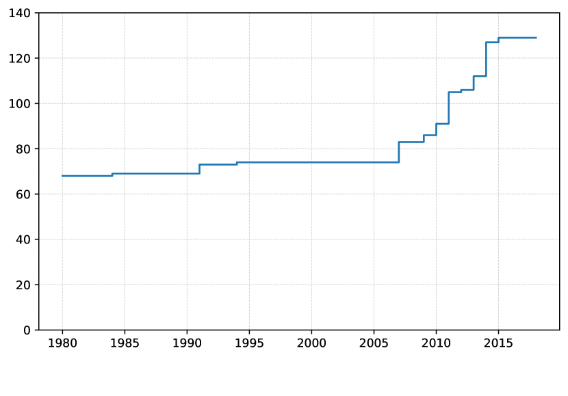
(a) Number of variables.

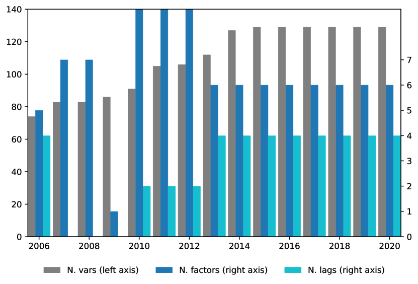
(b) Number of variables, factors and lags.

Figure 4: Panel (a) reports the number of variables along the entire time span taken into consideration. Panel (b) reports the number of variables, factors and lags selected via cross-validation over time. The blue line is the number of variables available for each year (left axis), red line is the optimal number of latent common states (right axis), black line is the optimal number of lags of input variables (right axis). The x-axis shows the year during which the model is used for the out-of-sample evaluation.

6.1 A Real-Time ‘Big’ Macro Dataset

To test its capability, we estimate the model by encoding a real-time version of the full McCracken and Ng (2016)’s FRED-MD dataset, a large macroeconomic database for the US economy, specifically designed for the empirical analysis of ‘big data’. The cross-section of data is mixed frequency because it includes 128 monthly indicators and Real GDP, that is a quarterly variable. All the data are stationarised and standardised following the specifications in McCracken and Ng (2016). In Tables 7-10, we report also the respective publication delay (in days) of each series. There are substantial differences in the timeliness of different variables. Some of them are more timely (e.g. ‘soft’ indicators or surveys), while others are released with one-two months of delay (usually ‘hard’ data on real activity).

The vintages in the datasets span the period from January 1980 to May 2020. Figure 4(a) reports the number of variables available across time periods. We first estimate the model using the data up to December 2005, and then we perform an expanding window forecasting exercise starting form the 1${}^{\text{st}}$ of January 2006. Hence our test sample goes from 1${}^{\text{st}}$ of January 2006 to 31${}^{\text{st}}$ of May 2020, including the Great Recession in 2007-2009. A data vintage is created every time a new time-series data point is released, and it contains all the data available up to that point in time, including also data revisions. The real-time infrastructure adapts automatically to the expanding number of variables used as input for the model. For each iteration, as new data arrive, the model is re-evaluated and outputs a sequence of backcasts-nowcasts-forecasts for GDP and all the other variables. These forecasts are conditional only to the real-time information set, i.e. only data available up to that specific point in time without taking into consideration further revisions.

Many of the hyperparameters of the model are not fixed ex-ante but are instead selected using an intensive cross-validation exercise, as reported in Table 4. The real-time cross-validation exercise also provides information on the ability of the model to update its optimal hyperparameter specification over time, as new data comes in (the validation length is set to one year). Figure 4(b) shows the evolution of the number of factors and lags that are selected via cross-validation over the sample.

6.2 Model Evaluation

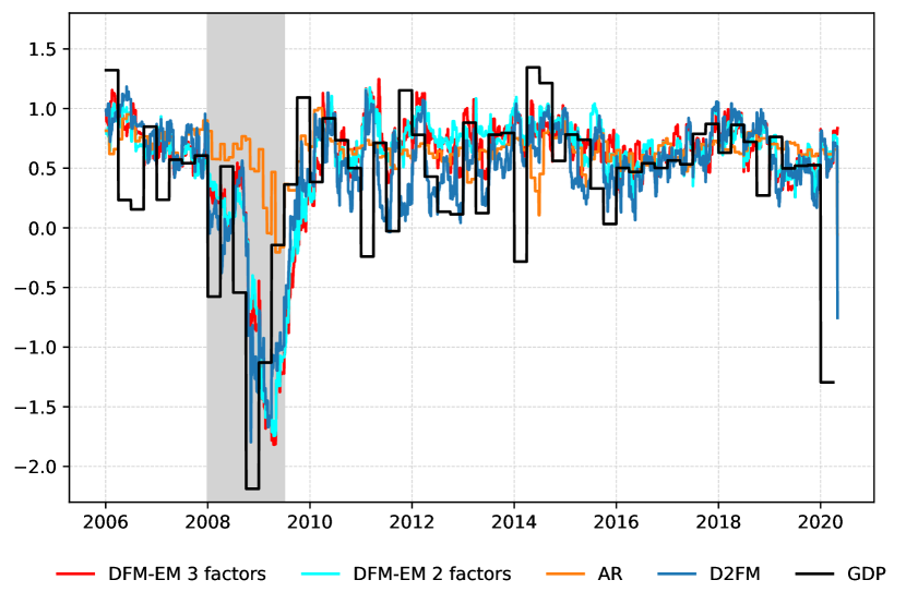
Figure 5: This Figure shows the nowcast reconstruction in real-time of the D²FM, DFM-EM with 2 and 3 factors and the AR(1) versus the growth rate of the US GDP. Shaded area is the NBER recession period.

Figure 5 shows the nowcast reconstruction in real-time for the D²FM, the DFM-EM with 2 and 3 factors, and the AR(1) model against the realised quarterly US GDP. Overall, the D²FM and the DFM-EM models provide a similar assessment of the state of the economy, in the nowcasting horizon, though the D²FM is more accurate.

Table 5: Comparison of RMSEs relative to the AR(1) benchmark

	Forecasting		Nowcasting			Backcasting
Model	30 weeks	26 weeks	20 weeks	14 weeks	8 weeks	2 weeks
D2FM	0.895	0.906	0.895	0.798	0.839	0.832
DFM-EM 3 factors	1.032	1.034	0.973	0.87	0.869	0.826
DFM-EM 2 factors	1.015	1.027	0.962	0.894	0.886	0.858

• Notes: This table reports the RMSE of the D²FM, the DFM-EM model with 2 and 3 factors relative to the RMSE of the AR(1): $RMSE(model,horizon)/RMSE(AR(1),horizon)$. Relative RMSEs are reported for different dates relative to the release date of US GDP. For example, the RMSEs at 30 weeks refers to the RMSEs 30 weeks prior to the release date.

We formally assess the performances of the model – and of the AR(1), the DFM-EM with 2 and 3 factors – by computing root mean square forecast error (RMSFE). This metric is updated every time the data vintage gets updated, due to a new data release. We report both an overall RMSFE (Table 5) that gives us a synthetic value about the performance of each model on the entire out-of-sample set, and a dynamic RMSFE (Figure 6) that illustrates how the RMSFE evolves from the forecast period to the backcast period, until the day before the release. Results indicate that the D²FM is able to outperform all the competitors during the entire forecast period and for most of the nowcast period. The gain in terms of performance achieved by the D²FM in these two periods is quite considerable and reflects the ability of this model to better compress the relevant information in the data, thus reducing the level of uncertainty.

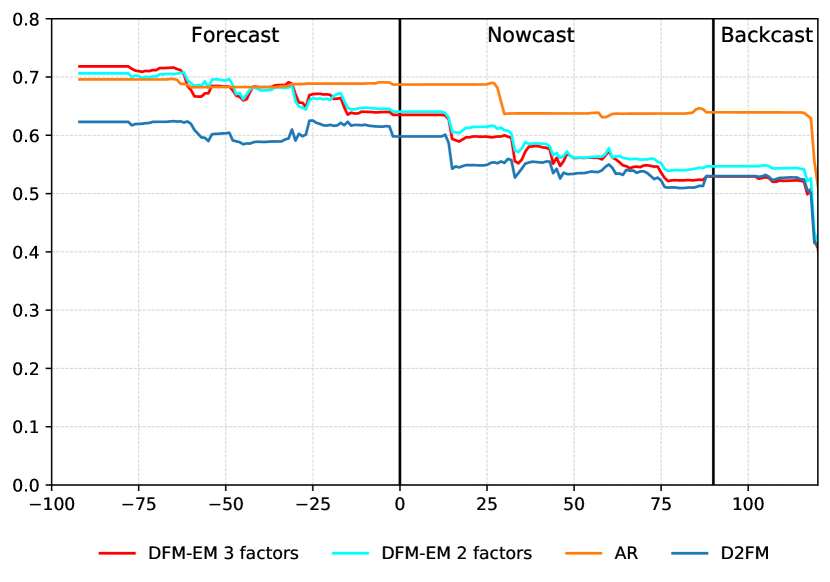
Figure 6: This Figure reports the RMSFE evolution along the quarter of the D²FM model versus its competitors.

The model also delivers forecasts for all the variables in the model. Table 6 reports the average of the RMSFEs of the D²FM over all of the monthly variables, in ratio to the AR(1) RMSFEs. The D²FM beats the AR(1) over all the horizons – the backcast improves by $10\%$, the nowcast improves by $20\%$ and the forecast improves by $18\%$.

Table 6: Comparison of RMSEs relative to the AR(1) benchmark for monthly variables.

	Forecasting			Nowcasting			Backcasting
		6 weeks			4 weeks			2 weeks
D2FM		0.85			0.83			0.91

• Notes: This table reports the average RMSFE of the D²FM model relative to the RMSFE of the AR(1) across all monthly variables included in the model. Relative RMSEs are reported for different dates relative to the release date of the monthly variables. For example, the RMSEs at 6 weeks refers to the RMSEs 6 weeks prior to the release date of the variable under consideration.

6.3 A Real-Time Synthetic Indicator of the Business Cycle

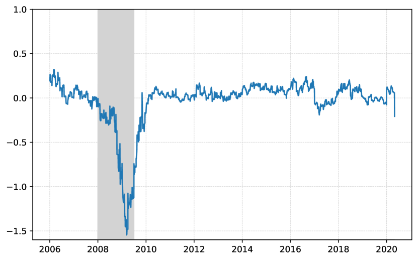
Figure 7: This Figure reports the Composite Indicator computed in real time using the D²FM of section 6.2.

As a final exercise, we show how to build a composite indicator of the state of economy in real-time using the decoding map (or loadings). We do this by aggregating the latent states trough a weighting scheme. Specifically, we define the composite indicator as

$$CI=\sum_{k=1}^{r}\sum_{i=1}^{N}f_{k}\frac{F_{k,i}^{2}}{||F||_{F}^{2}}\ ,$$ (29)

where $f_{k}$ for $k=1,...,r$ are the common factors (the code) and $F_{k,i}$ is the matrix of the coefficient for the factor $k$ at variable $i$, as in the Equation 14^′, while $||F||_{F}^{2}=\sum_{k=1}^{r}\sum_{i=1}^{n}F_{k,i}^{2}$ is the squared Frobenius norm of the coefficients. The sign of the indicator is fixed to have a positive correlation with GDP. Figure 7 reports the composite indicator using the real time out of sample exercise, that is shown to track well the developments in the US economy.

7 Conclusion

The central contribution of our paper is to introduce Deep Dynamic Factor Models (D²FMs) by showing how to embed autoencoders in a dynamic nonlinear factor model structure with idiosyncratic components. The equivalence between maximum likelihood estimation and minimisation of mean squared error, together with the Universal Approximation Theorem allow to conceptualise the D²FMs as computationally efficient approximations of the maximum likelihood estimates of generic nonlinear factor models.

The application of a simple version of our D²FM with linear dynamic equations and a linear decoder, both in a Monte Carlo experiment, and in a big data real-time forecasting exercise shows the potential of the methodology.

The model capability can be further generalised and employed in multiple directions. For example, one could consider empirical applications that consider a nonlinear decoding structure, or nonlinear dynamic equations for the factors. Also, the loss function could be changed to allow for quantile estimates (see Koenker and Bassett, 1978; Chen et al., 2018, for example). Finally, it is worth observing that the modularity and flexibility of the D²FM allow to easily integrate alternative data (e.g. text data, satellite images, micro-data, etc) into the model. We leave these promising avenues of research to the future.

Appendix A Data Appendix

Tables 7-10 reports the list of variables in the dataset. The transformation codes (Tcode) in the Tables refers to how the variables are transformed to archive stationarity stationary. Being $X_{t}$ a raw series, the transformations adopted are:

$$Z_{t}=\begin{cases}X_{t}&\mbox{if Tcode}=1\\ (1-L)X_{t}&\mbox{if Tcode}=2\\ (1-L)(1-L^{12})X_{t}&\mbox{if Tcode}=3\\ \mbox{log}X_{t}&\mbox{if Tcode}=4\\ (1-L)\mbox{log}X_{t}&\mbox{if Tcode}=5\\ (1-L)(1-L^{12})\mbox{log}X_{t}&\mbox{if Tcode}=6\\ \end{cases}$$

Table 7: Dataset (I)

N	Code	Descriptions	Source	Tcode	Freq	McCracken gr	Publication delay
1	RPI	Real Personal Income	FRED	5	M	1	30
2	W875RX1	RPI ex. Transfers	FRED	5	M	1	30
3	INDPRO	IP Index	FRED	5	M	1	14
4	IPFPNSS	IP: Final Products and Supplies	FRED	5	M	1	14
5	IPFINAL	IP: Final Products	FRED	5	M	1	14
6	IPCONGD	IP: Consumer Goods	FRED	5	M	1	14
7	IPDCONGD	IP: Durable Consumer Goods	FRED	5	M	1	14
8	IPNCONGD	IP: Nondurable Consumer Goods	FRED	5	M	1	14
9	IPBUSEQ	IP: Business Equipment	FRED	5	M	1	14
10	IPMAT	IP: Materials	FRED	5	M	1	14
11	IPDMAT	IP: Durable Materials	FRED	5	M	1	14
12	IPNMAT	IP: Nondurable Materials	FRED	5	M	1	14
13	IPMANSICS	IP: Manufacturing	FRED	5	M	1	14
14	IPB51222S	IP: Residential Utilities	FRED	5	M	1	14
15	IPFUELS	IP: Fuels	FRED	5	M	1	14
16	CLF16OV	Civilian Labor Force	FRED	5	M	2	7
17	CE16OV	Civilian Employment	FRED	5	M	2	7
18	UNRATE	Civilian Unemployment Rate	FRED	2	M	2	7
19	UEMPMEAN	Average Duration of Unemployment	FRED	2	M	2	7
20	UEMPLT5	Civilians Unemployed ¡5 Weeks	FRED	5	M	2	7
21	UEMP5TO14	Civilians Unemployed 5-14 Weeks	FRED	5	M	2	7
22	UEMP15OV	Civilians Unemployed ¿15 Weeks	FRED	5	M	2	7
23	UEMP15T26	Civilians Unemployed 15-26 Weeks	FRED	5	M	2	7
24	UEMP27OV	Civilians Unemployed ¿27 Weeks	FRED	5	M	2	7
25	PAYEMS	All Employees: Total nonfarm	FRED	5	M	2	7
26	USGOOD	All Employees: Goods-Producing	FRED	5	M	2	7
27	CES1021000001	All Employees: Mining and Logging	FRED	5	M	2	7
28	USCONS	All Employees: Construction	FRED	5	M	2	7
29	MANEMP	All Employees: Manufacturing	FRED	5	M	2	7
30	DMANEMP	All Employees: Durable goods	FRED	5	M	2	7
31	NDMANEMP	All Employees: Nondurable goods	FRED	5	M	2	7
32	SRVPRD	All Employees: Service Industries	FRED	5	M	2	7
33	USTPU	All Employees: TT&U	FRED	5	M	2	7

Table 8: Dataset (II)

N	Code	Descriptions	Source	Tcode	Freq	McCracken gr	Publication delay
34	USWTRADE	All Employees: Wholesale Trade	FRED	5	M	2	7
35	USTRADE	All Employees: Retail Trade	FRED	5	M	2	7
36	USFIRE	All Employees: Financial Activities	FRED	5	M	2	7
37	USGOVT	All Employees: Government	FRED	5	M	2	7
38	CES0600000007	Hours: Goods-Producing	FRED	1	M	2	7
39	AWOTMAN	Overtime Hours: Manufacturing	FRED	2	M	2	7
40	AWHMAN	Hours: Manufacturing	FRED	1	M	2	7
41	CES0600000008	Ave. Hourly Earnings: Goods	FRED	6	M	2	7
42	CES2000000008	Ave. Hourly Earnings: Construction	FRED	6	M	2	7
43	CES3000000008	Ave. Hourly Earnings: Manufacturing	FRED	6	M	2	7
44	HOUST	Starts: Total	FRED	4	M	3	20
45	HOUSTNE	Starts: Northeast	FRED	4	M	3	20
46	HOUSTMW	Starts: Midwest	FRED	4	M	3	20
47	HOUSTS	Starts: South	FRED	4	M	3	20
48	HOUSTW	Starts: West	FRED	4	M	3	20
49	PERMIT	Permits	FRED	4	M	3	20
50	PERMITNE	Permits: Northeast	FRED	4	M	3	20
51	PERMITMW	Permits: Midwest	FRED	4	M	3	20
52	PERMITS	Permits: South	FRED	4	M	3	20
53	PERMITW	Permits: West	FRED	4	M	3	20
54	DPCERA3M086SBEA	Real PCE	FRED	5	M	4	30
55	CMRMTSPL	Real M&T Sales	FRED	5	M	4	35
56	RETAIL	Retail and Food Services Sales	FRED	5	M	4	30
57	ACOGNO	Orders: Consumer Goods	FRED	5	M	4	35
58	ANDENO	Orders: Nondefense Capital Goods	FRED	5	M	4	35
59	AMDMUO	Unfilled Orders: Durable Goods	FRED	5	M	4	35
60	BUSINV	Total Business Inventories	FRED	5	M	4	35
61	ISRATIO	Inventories to Sales Ratio	FRED	2	M	4	35
62	UMCSENT	Consumer Sentiment Index	FRED	2	M	4	-3
63	M1SL	M1 Money Stock	FRED	6	M	5	14
64	M2SL	M2 Money Stock	FRED	6	M	5	14
65	M3SL	MABMM301USM189S in FRED, M3 for the United States	FRED	6	M	5	14
66	M2REAL	Real M2 Money Stock	FRED	5	M	5	14

Table 9: Dataset (III)

N	Code	Descriptions	Source	Tcode	Freq	McCracken gr	Publication delay
67	AMBSL	St. Louis Adjusted Monetary Base	FRED	6	M	5	14
68	TOTRESNS	Total Reserves	FRED	6	M	5	36
69	NONBORRES	Nonborrowed Reserves	FRED	0	M	5	36
70	BUSLOANS	Commercial and Industrial Loans	FRED	6	M	5	20
71	REALLN	Real Estate Loans	FRED	1	M	5	20
72	NONREVSL	Total Nonrevolving Credit	FRED	6	M	5	14
73	MZMSL	MZM Money Stock	FRED	6	M	5	14
74	DTCOLNVHFNM	Consumer Motor Vehicle Loans	FRED	6	M	5	14
75	DTCTHFNM	Total Consumer Loans and Leases	FRED	6	M	5	14
76	INVEST	Securities in Bank Credit	FRED	6	M	5	14
77	FEDFUNDS	Effective Federal Funds Rate	FRED	2	M	6	-1
78	CP3M	3-Month AA Comm. Paper Rate	FRED	2	M	6	0
79	TB3MS	3-Month T-bill	FRED	2	M	6	0
80	TB6MS	6-Month T-bill	FRED	2	M	6	0
81	GS1	1-Year T-bond	FRED	2	M	6	0
82	GS5	5-Year T-bond	FRED	2	M	6	0
83	GS10	10-Year T-bond	FRED	2	M	6	0
84	AAA	Aaa Corporate Bond Yield	FRED	2	M	6	2
85	BAA	Baa Corporate Bond Yield	FRED	2	M	6	2
86	TB3SMFFM	3 Mo. - FFR spread	FRED	1	M	6	2
87	TB6SMFFM	6 Mo. - FFR spread	FRED	1	M	6	2
88	T1YFFM	1 yr. - FFR spread	FRED	1	M	6	2
89	T5YFFM	5 yr. - FFR spread	FRED	1	M	6	2
90	T10YFFM	10 yr. - FFR spread	FRED	1	M	6	0
91	AAAFFM	Aaa - FFR spread	FRED	1	M	6	0
92	BAAFFM	Baa - FFR spread	FRED	1	M	6	0
93	TWEXMMTH	Trade Weighted U.S. FX Rate	FRED	5	M	6	2
94	EXSZUS	Switzerland / U.S. FX Rate	FRED	5	M	6	2
95	EXJPUS	Japan / U.S. FX Rate	FRED	5	M	6	2
96	EXUSUK	U.S. / U.K. FX Rate	FRED	5	M	6	2
97	EXCAUS	Canada / U.S. FX Rate	FRED	5	M	6	2
98	PPIFGS	PPI: Finished Goods	FRED	6	M	7	16
99	PPIFCG	PPI: Finished Consumer Goods	FRED	6	M	7	16

Table 10: Dataset (IV)

N	Code	Descriptions	Source	Tcode	Freq	McCracken gr	Publication delay
100	PPIITM	PPI: Intermediate Materials	FRED	6	M	7	16
101	PPICRM	PPI: Crude Materials	FRED	6	M	7	16
102	oilprice	Crude Oil Prices: WTI	HAVER	6	M	7	0
103	PPICMM	PPI: Commodities	FRED	6	M	7	16
104	CPIAUCSL	CPI: All Items	FRED	6	M	7	16
105	CPIAPPSL	CPI: Apparel	FRED	6	M	7	16
106	CPITRNSL	CPI: Transportation	FRED	6	M	7	16
107	CPIMEDSL	CPI: Medical Care	FRED	6	M	7	16
108	CUSR0000SAC	CPI: Commodities	FRED	6	M	7	16
109	CUUR0000SAD	CPI: Durables	FRED	6	M	7	16
110	CUSR0000SAS	CPI: Services	FRED	6	M	7	16
111	CPIULFSL	CPI: All Items Less Food	FRED	6	M	7	16
112	CUUR0000SA0L2	CPI: All items less shelter	FRED	6	M	7	16
113	CUSR0000SA0L5	CPI: All items less medical care	FRED	6	M	7	16
114	PCEPI	PCE: Chain-type Price Index	FRED	6	M	7	30
115	DDURRG3M086SBEA	PCE: Durable goods	FRED	6	M	7	30
116	DNDGRG3M086SBEA	PCE: Nondurable goods	FRED	6	M	7	30
117	DSERRG3M086SBEA	PCE: Services	FRED	6	M	7	30
118	IPMAN	Industrial Production: Manufacturing	FRED	1	M	1	14
119	MCUMFN	Capacity Utilization: Manufacturing	FRED	2	M	1	14
120	TCU	Capacity Utilization: Total Industry	FRED	2	M	1	14
121	M0684AUSM343SNBR	Manufacturers’ Index of New Orders of Durable Goods	FRED	1	M	4	34
122	M0504AUSM343SNBR	Manufacturers’ Inventories, Total for United States	FRED	1	M	4	34
123	DGORDER	Manufacturers’ New Orders: Durable Goods	FRED	5	M	4	34
124	CPFFM	3-Month Commercial Paper Minus Federal Funds Rate	FRED	1	M	6	0
125	PCUOMFGOMFG	Producer Price Index by Industry: Total Manufacturing	FRED	1	M	7	15
126	ISMC	ISM Composite Index	HAVER	1	M	1	3
127	NAPMVDI	ISM Manufacturing: Supply Index	HAVER	1	M	1	3
128	SP500E	Standard & poor 500: Price Index	HAVER	5	M	8	0
129	SDY5COMM	Standard & poor 500: Dividend Yield	HAVER	2	M	8	0
130	SPE5COOM	Standard & poor 500: Price/Earnings Ratio	HAVER	5	M	8	0
131	GDPC1	Gross Domestic Product	FRED	5	Q	1	30

References

- (1)
- Alessi et al. (2010) Alessi, Lucia, Matteo Barigozzi, and Marco Capasso, “Improved penalization for determining the number of factors in approximate factor models,” Statistics & Probability Letters, 2010, 80 (23-24), 1806–1813.
- Altissimo et al. (2010) Altissimo, Filippo, Riccardo Cristadoro, Mario Forni, Marco Lippi, and Giovanni Veronese, “New Eurocoin: Tracking economic growth in real time,” The review of economics and statistics, 2010, 92 (4), 1024–1034.
- Amisano and Tristani (2011) Amisano, Gianni and Oreste Tristani, “Exact likelihood computation for nonlinear DSGE models with heteroskedastic innovations,” Journal of Economic Dynamics and Control, 2011, 35 (12), 2167–2185.
- Bai and Ng (2002) Bai, Jushan and Serena Ng, “Determining the number of factors in approximate factor models,” Econometrica, 2002, 70 (1), 191–221.
- Bai and Ng (2008) and , “Forecasting economic time series using targeted predictors,” Journal of Econometrics, 2008, 146 (2), 304 – 317. Honoring the research contributions of Charles R. Nelson.
- Baldi and Hornik (1989) Baldi, Pierre and Kurt Hornik, “Neural networks and principal component analysis: Learning from examples without local minima,” Neural networks, 1989, 2 (1), 53–58.
- Banbura and Modugno (2014) Banbura, Marta and Michele Modugno, “Maximum likelihood estimation of factor models on datasets with arbitrary pattern of missing data,” Journal of Applied Econometrics, 2014, 29 (1), 133–160.
- Banbura et al. (2010) , Domenico Giannone, and Lucrezia Reichlin, “Nowcasting,” ECB working paper, 2010.
- Barigozzi and Luciani (2019) Barigozzi, Matteo and Matteo Luciani, “Quasi Maximum Likelihood Estimation and Inference of Large Approximate Dynamic Factor Models via the EM algorithm,” arXiv preprint arXiv:1910.03821, 2019.
- Barnett et al. (2016) Barnett, William A., Marcelle Chauvet, and Danilo Leiva-Leon, “Real-time nowcasting of nominal GDP with structural breaks,” Journal of Econometrics, 2016, 191 (2), 312–324.
- Bengio et al. (2013) Bengio, Yoshua, Li Yao, Guillaume Alain, and Pascal Vincent, “Generalized denoising auto-encoders as generative models,” in “Advances in neural information processing systems” 2013, pp. 899–907.
- Bergmeir et al. (2018) Bergmeir, Christoph, Rob J. Hyndman, and Bonsoo Koo, “A note on the validity of cross-validation for evaluating autoregressive time series prediction,” Computational Statistics & Data Analysis, 2018, 120, 70–83.
- Bergstra et al. (2011) Bergstra, James S., Rémi Bardenet, Yoshua Bengio, and Balázs Kégl, “Algorithms for Hyper-Parameter Optimization,” 2011, pp. 2546–2554.
- Blasques et al. (2016) Blasques, Francisco, Siem Jan Koopman, Max Mallee, and Zhaoyong Zhang, “Weighted maximum likelihood for dynamic factor analysis and forecasting with mixed frequency data,” Journal of Econometrics, 2016, 193 (2), 405–417.
- Bourlard and Kamp (1988) Bourlard, Hervé and Yves Kamp, “Auto-association by multilayer perceptrons and singular value decomposition,” Biological cybernetics, 1988, 59 (4-5), 291–294.
- Burns and Mitchell (1946) Burns, Arthur F. and Wesley C. Mitchell, Measuring Business Cycles number burn46-1. In ‘NBER Books.’, National Bureau of Economic Research, Inc, July 1946.
- Camacho et al. (2012) Camacho, Maximo, Gabriel Perez-Quiros, and Pilar Poncela, “Markov-switching dynamic factor models in real time,” 2012.
- Cauchy (1847) Cauchy, Augustin, “Méthode générale pour la résolution des systemes d’équations simultanées,” Comp. Rend. Sci. Paris, 1847, 25 (1847), 536–538.
- Chen et al. (2018) Chen, Liang, Juan Dolado, and Jesus Gonzalo, “Quantile factor models,” 2018.
- Cook and Hall (2017) Cook, Thomas and Aaron Smalter Hall, “Macroeconomic indicator forecasting with deep neural networks,” Federal Reserve Bank of Kansas City, Research Working Paper, 2017, (17-11).
- Cybenko (1989) Cybenko, George, “Approximation by superpositions of a sigmoidal function,” Mathematics of control, signals and systems, 1989, 2 (4), 303–314.
- Dempster et al. (1977) Dempster, Arthur P., Nan M. Laird, and Donald B. Rubin, “Maximum likelihood from incomplete data via the EM algorithm,” Journal of the Royal Statistical Society: Series B (Methodological), 1977, 39 (1), 1–22.
- Doz et al. (2012) Doz, Catherine, Domenico Giannone, and Lucrezia Reichlin, “A quasi–maximum likelihood approach for large, approximate dynamic factor models,” Review of economics and statistics, 2012, 94 (4), 1014–1024.
- Duchi et al. (2011) Duchi, John, Elad Hazan, and Yoram Singer, “Adaptive subgradient methods for online learning and stochastic optimization,” Journal of machine learning research, 2011, 12 (Jul), 2121–2159.
- Engle and Watson (1981) Engle, Robert and Mark W. Watson, “A one-factor multivariate time series model of metropolitan wage rates,” Journal of the American Statistical Association, 1981, 76 (376), 774–781.
- Forni et al. (2018) Forni, Mario, Alessandro Giovannelli, Marco Lippi, and Stefano Soccorsi, “Dynamic factor model with infinite-dimensional factor space: Forecasting,” Journal of Applied Econometrics, 2018, 33 (5), 625–642.
- Forni and Reichlin (1998) and Lucrezia Reichlin, “Let’s get real: a factor analytical approach to disaggregated business cycle dynamics,” The Review of Economic Studies, 1998, 65 (3), 453–473.
- Forni and Lippi (2001) and Marco Lippi, “The generalized dynamic factor model: representation theory,” Econometric theory, 2001, 17 (6), 1113–1141.
- Forni et al. (2000) , Marc Hallin, Marco Lippi, and Lucrezia Reichlin, “The generalized dynamic-factor model: Identification and estimation,” Review of Economics and statistics, 2000, 82 (4), 540–554.
- Forni et al. (2005) , , , and , “The generalized dynamic factor model: one-sided estimation and forecasting,” Journal of the American Statistical Association, 2005, 100 (471), 830–840.
- Forni et al. (2015) , , , and Paolo Zaffaroni, “Dynamic factor models with infinite-dimensional factor spaces: One-sided representations,” Journal of econometrics, 2015, 185 (2), 359–371.
- Foroni and Marcellino (2013) Foroni, Claudia and Massimiliano Giuseppe Marcellino, “A survey of econometric methods for mixed-frequency data,” Available at SSRN 2268912, 2013.
- Fraccaro et al. (2017) Fraccaro, Marco, Simon Kamronn, Ulrich Paquet, and Ole Winther, “A disentangled recognition and nonlinear dynamics model for unsupervised learning,” in “Advances in Neural Information Processing Systems” 2017, pp. 3601–3610.
- Geweke (1977) Geweke, John, “The dynamic factor analysis of economic time series,” Latent Variables in Socio-Economic Models, 1977.
- Giannone et al. (2008) Giannone, Domenico, Lucrezia Reichlin, and David Small, “Nowcasting: The real-time informational content of macroeconomic data,” Journal of Monetary Economics, 2008, 55 (4), 665–676.
- Glorot and Bengio (2010) Glorot, Xavier and Yoshua Bengio, “Understanding the difficulty of training deep feedforward neural networks,” in “Proceedings of the thirteenth international conference on artificial intelligence and statistics” 2010, pp. 249–256.
- Goodfellow et al. (2016) Goodfellow, Ian, Yoshua Bengio, and Aaron Courville, “Deep Learning,” MIT Press, 2016, p. 800.
- Gregor et al. (2019) Gregor, Karol, George Papamakarios, Frederic Besse, Lars Buesing, and Theophane Weber, “Temporal Difference Variational Auto-Encoder,” in “International Conference on Learning Representations” 2019.
- Gregor et al. (2014) , Ivo Danihelka, Andriy Mnih, Charles Blundell, and Daan Wierstra, “Deep AutoRegressive Networks,” in “Proceedings of the 31st International Conference on Machine Learning,” Vol. 32 of Proceedings of Machine Learning Research PMLR 2014, pp. 1242–1250.
- Gu et al. (2018) Gu, Shihao, Bryan Kelly, and Dacheng Xiu, “Empirical asset pricing via machine learning,” National Bureau of Economic Research, 2018.
- Gu et al. (2019) , Bryan T. Kelly, and Dacheng Xiu, “Autoencoder asset pricing models,” Available at SSRN, 2019.
- Heaton et al. (2016) Heaton, JB, Nicholas G. Polson, and Jan Hendrik Witte, “Deep learning in finance,” arXiv preprint arXiv:1602.06561, 2016.
- Hinton and Zemel (1994) Hinton, Geoffrey E. and Richard S. Zemel, “Autoencoders, minimum description length and Helmholtz free energy,” in “Advances in neural information processing systems” 1994, pp. 3–10.
- Hinton and Salakhutdinov (2006) and Ruslan R. Salakhutdinov, “Reducing the dimensionality of data with neural networks,” science, 2006, 313 (5786), 504–507.
- Holopainen and Sarlin (2017) Holopainen, Markus and Peter Sarlin, “Toward robust early-warning models: A horse race, ensembles and model uncertainty,” Quantitative Finance, 2017, 17 (12), 1933–1963.
- Hornik et al. (1989) Hornik, Kurt, Maxwell Stinchcombe, and Halbert White, “Multilayer feedforward networks are universal approximators,” Neural Networks, 1989, 2 (5), 359 – 366.
- Hornik et al. (1990) , , and , “Universal approximation of an unknown mapping and its derivatives using multilayer feedforward networks,” Neural Networks, 1990, 3 (5), 551 – 560.
- Ioffe and Szegedy (2015) Ioffe, Sergey and Christian Szegedy, “Batch Normalization: Accelerating Deep Network Training by Reducing Internal Covariate Shift,” in Francis Bach and David Blei, eds., Proceedings of the 32nd International Conference on Machine Learning, Vol. 37 of Proceedings of Machine Learning Research PMLR Lille, France 07–09 Jul 2015, pp. 448–456.
- Japkowicz et al. (2000) Japkowicz, Nathalie, Stephen Jose Hanson, and Mark A Gluck, “Nonlinear autoassociation is not equivalent to PCA,” Neural computation, 2000, 12 (3), 531–545.
- Johnson et al. (2016) Johnson, Matthew J, David K Duvenaud, Alex Wiltschko, Ryan P Adams, and Sandeep R Datta, “Composing graphical models with neural networks for structured representations and fast inference,” in D. D. Lee, M. Sugiyama, U. V. Luxburg, I. Guyon, and R. Garnett, eds., Advances in Neural Information Processing Systems 29, Curran Associates, Inc., 2016, pp. 2946–2954.
- Kiefer and Wolfowitz (1952) Kiefer, Jack and Jacob Wolfowitz, “Stochastic estimation of the maximum of a regression function,” The Annals of Mathematical Statistics, 1952, 23 (3), 462–466.
- Kingma and Ba (2014) Kingma, Diederik and Jimmy Ba, “Adam: A Method for Stochastic Optimization,” International Conference on Learning Representations, 2014.
- Kock et al. (2011) Kock, Anders Bredahl, Timo Teräsvirta et al., “Forecasting with nonlinear time series models,” Oxford handbook of economic forecasting, 2011, pp. 61–87.
- Koenker and Bassett (1978) Koenker, Roger and Gilbert Jr Bassett, “Regression quantiles,” Econometrica: journal of the Econometric Society, 1978, pp. 33–50.
- Korobilis (2006) Korobilis, Dimitris, “Forecast comparison of nonlinear time series models of US GDP: A Bayesian approach,” Available at SSRN 1508486, 2006.
- Krishnan et al. (2017) Krishnan, Rahul G., Uri Shalit, and David Sontag, “Structured Inference Networks for Nonlinear State Space Models,” in “Proceedings of the Thirty-First AAAI Conference on Artificial Intelligence” AAAI’17 AAAI Press 2017, p. 2101–2109.
- LeCun (1987) LeCun, Yann, “PhD thesis: Modeles connexionnistes de l’apprentissage (connectionist learning models),” 1987.
- Loermann and Maas (2019) Loermann, Julius and Benedikt Maas, “Nowcasting US GDP with artificial neural networks,” Munich Personal RePEc Archive, 2019.
- Lu et al. (2017) Lu, Zhou, Hongming Pu, Feicheng Wang, Zhiqiang Hu, and Liwei Wang, “The expressive power of neural networks: A view from the width,” in “Advances in neural information processing systems” 2017, pp. 6231–6239.
- Majumdar and Tripathi (2017) Majumdar, Angshul and Aditay Tripathi, “Asymmetric stacked autoencoder,” in “in” IEEE 2017 International Joint Conference on Neural Networks (IJCNN) 2017, pp. 911–918.
- Marcellino and Schumacher (2010) Marcellino, Massimiliano and Christian Schumacher, “Factor MIDAS for nowcasting and forecasting with ragged-edge data: A model comparison for German GDP,” Oxford Bulletin of Economics and Statistics, 2010, 72 (4), 518–550.
- Mariano and Murasawa (2003) Mariano, Roberto S. and Yasutomo Murasawa, “A new coincident index of business cycles based on monthly and quarterly series,” Journal of applied Econometrics, 2003, 18 (4), 427–443.
- McCracken and Ng (2016) McCracken, Michael W. and Serena Ng, “FRED-MD: A monthly database for macroeconomic research,” Journal of Business & Economic Statistics, 2016, 34 (4), 574–589.
- Nakajima and West (2013) Nakajima, Jouchi and Mike West, “Bayesian analysis of latent threshold dynamic models,” Journal of Business & Economic Statistics, 2013, 31 (2), 151–164.
- Rangapuram et al. (2018) Rangapuram, Syama Sundar, Matthias W Seeger, Jan Gasthaus, Lorenzo Stella, Yuyang Wang, and Tim Januschowski, “Deep state space models for time series forecasting,” in “Advances in neural information processing systems” 2018, pp. 7785–7794.
- Rudin (2019) Rudin, Cynthia, “Stop explaining black box machine learning models for high stakes decisions and use interpretable models instead,” Nature Machine Intelligence, 2019, 1 (5), 206–215.
- Rumelhart et al. (1986) Rumelhart, David E., Geoffrey E. Hinton, and Ronald J. Williams, “Learning representations by back-propagating errors,” nature, 1986, 323 (6088), 533–536.
- Sargent and Sims (1977) Sargent, Thomas and C.A. Sims, “Business Cycle Modeling Without Pretending to Have Too Much a Priori Economic Theory,” 10 1977, pp. 45–109.
- Sezer et al. (2019) Sezer, Omer Berat, Mehmet Ugur Gudelek, and Ahmet Murat Ozbayoglu, “Financial Time Series Forecasting with Deep Learning: A Systematic Literature Review: 2005-2019,” arXiv preprint arXiv:1911.13288, 2019.
- Shumway and Stoffer (1982) Shumway, Robert H. and David S. Stoffer, “An approach to time series smoothing and forecasting using the EM algorithm,” Journal of time series analysis, 1982, 3 (4), 253–264.
- Stevens and Antiga (2019) Stevens, Eli and Luca Antiga, Deep Learning with PyTorch, Manning Publications, 2019.
- Stock and Watson (1989) Stock, James H. and Mark W. Watson, “New indexes of coincident and leading economic indicators,” NBER macroeconomics annual, 1989, 4, 351–394.
- Stock and Watson (2002a) and , “Forecasting using principal components from a large number of predictors,” Journal of American Statistical Association, 2002, 97, 1167–1179.
- Stock and Watson (2002b) and , “Macroeconomic forecasting using diffusion indexes,” Journal of Business Economics and Statistics, 2002, 20, 147–162.
- Stock and Watson (2011) and , “Dynamic factor models,” Oxford Handbooks Online, 2011.
- Stock and Watson (2016) and , “Chapter 8 - Dynamic Factor Models, Factor-Augmented Vector Autoregressions, and Structural Vector Autoregressions in Macroeconomics,” in John B. Taylor and Harald Uhlig, eds., John B. Taylor and Harald Uhlig, eds., Vol. 2 of Handbook of Macroeconomics, Elsevier, 2016, pp. 415 – 525.
- Tieleman and Hinton (2012) Tieleman, Tijmen and Geoffrey Hinton, “RMSProp,” COURSERA: Lecture, 2012, 7017.
- Vincent et al. (2008) Vincent, Pascal, Hugo Larochelle, Yoshua Bengio, and Pierre-Antoine Manzagol, “Extracting and composing robust features with denoising autoencoders,” in “in” Proceedings of the 25th international conference on Machine learning 2008, pp. 1096–1103.
- Watson and Engle (1983) Watson, Mark W. and Robert F. Engle, “Alternative algorithms for the estimation of dynamic factor, mimic and varying coefficient regression models,” Journal of Econometrics, 1983, 23 (3), 385–400.