institutetext: International School of Advanced Studies (SISSA), via Bonomea 265, 34136 Trieste, Italyinstitutetext: Institute for Geometry and Physics (IGAP), via Beirut 2/1, 34151 Trieste, Italyinstitutetext: INFN, Sezione di Trieste

BPS quivers of five-dimensional SCFTs, Topological Strings and q-Painlevé equations

Giulio Bonelli    Fabrizio Del Monte    and Alessandro Tanzini
Abstract

We study the discrete flows generated by the symmetry group of the BPS quivers for Calabi-Yau geometries describing five dimensional superconformal quantum field theories on a circle. These flows naturally describe the BPS particle spectrum of such theories and at the same time generate bilinear equations of q-difference type which, in the rank one case, are q-Painlevé equations. The solutions of these equations are shown to be given by grand canonical topological string partition functions which we identify with τ𝜏\tau-functions of the cluster algebra associated to the quiver. We exemplify our construction in the case corresponding to five dimensional SU(2)𝑆𝑈2SU(2) pure Super Yang-Mills and Nf=2subscript𝑁𝑓2N_{f}=2 on a circle.

1 Introduction

A crucial problem in quantum field theory (QFT) is understanding its non perturbative aspects in the concrete terms of exact computations. QFTs can be embedded in string theory/M-theory via geometric engineering hori2003mirror . Specifically, it can be obtained as the low energy limit of a compactified string theory in a large volume limit, which is needed to decouple its gravitational sector. When QFT is obtained in this way, the nature of exact dualities gets unveiled through the geometric properties of the string theory background behind it: the string theory on the non-compact Calabi-Yau (CY) background geometry encodes the spectral geometry of integrable systems whose solutions allow to obtain exact results. This is possible because the non-perturbative sector of string theory, described by D-branes, gets transferred through this procedure to the geometrically engineered QFT. The set-up engineered by M-theory compactification on CY3×S1𝐶subscript𝑌3superscript𝑆1CY_{3}\times S^{1}, in the limit of large CY3𝐶subscript𝑌3CY_{3} volume and finite S1superscript𝑆1S^{1} radius, is that of a five dimensional supersymmetric QFT on a circle, whose particles arise from membranes wrapped on the 2-cycles of a suitable non compact CY manifold. As such, the counting of the BPS protected sectors of the theory can be obtained by considering a dual picture given in terms of a topological string on CY3𝐶subscript𝑌3CY_{3}. The precise dictionary between the two descriptions is obtained by identifying the topological string partition function on the CY3𝐶subscript𝑌3CY_{3} with the supersymmetric index of the gauge theory, which is conjectured to capture the exact BPS content of its 5d SCFT completion Iqbal:2012xm . More generally, the supersymmetric index of the gauge theory with surface defects is matched with the corresponding D-brane open topological string wave function Aganagic:2003db ; Dijkgraaf:2007sw . The coupling constants and the moduli of the QFT arise from the geometric engineering as CY moduli parameters (Kähler and complex in the A and B-model picture respectively). Therefore, the QFT generated in this way is naturally in a generic phase in which all the coupling constants can be finite. To identify the weakly coupled regimes, one has to consider particular corners in the CY moduli space. In such corners, the topological string theory amplitudes allow a power expansion in at least one small parameter which is identified with the gauge coupling, while the others are fugacities of global symmetries of the QFT (masses and Coulomb parameters).

The problem we would like to face, in the general set-up described so far, is that of understanding how to predict the properties of such a supersymmetric index, given the non-compact CY manifold which realizes the five dimensional theory via geometric engineering. We will show that this index satisfies suitable q-difference equations which in the rank one case, namely for Calabi-Yaus whose mirror is a local genus one curve, are well-known in the mathematical physics literature as q-Painlevé equations 2001CMaPh.220..165S . These are classified in terms of their symmetry groups as in Fig. 1. Remarkably, this classification coincides with the one obtained from string theory considerations in Seiberg:1996bd . This allows to describe the grand canonical partition function of topological strings as τ𝜏\tau-functions of a discrete dynamical system, whose solutions encode the BPS spectrum of the theory. From this viewpoint the grand canonical partition function is actually vector-valued in the symmetry lattice of the discrete dynamical system at hand. The exact spectrum of the relevant integrable system can be computed from the zeros of the grand partition function.

The solutions of the discrete dynamical system are naturally parametrised in different ways according to the different BPS chambers of the theory. We will show that the Nekrasov-Okounkov Nekrasov:2003rj presentation of the supersymmetric index can be recovered in the large volume regions of the Calabi-Yau moduli space which allow the geometric engineering of five-dimensional gauge theories. The expansion parameter is schematically eVsuperscript𝑒𝑉e^{-V}, V𝑉V being the volume of the relevant cycle corresponding to the instanton counting parameter. Around the conifold point the solution is instead naturally parameterized in terms of a matrix model providing the non-perturbative completion of topological string via topological string/spectral theory correspondence Grassi:2014zfa . The case of local 𝔽0subscript𝔽0\mathbb{F}_{0} geometry, which engineers pure SU(2)𝑆𝑈2SU(2) Yang-Mills in five dimensions at zero Chern-Simons level, was discussed in detail in Bonelli:2017gdk . In this case the matrix model is a q-deformation of the O(2)𝑂2O(2) matrix model describing 2d Ising correlators Zamolodchikov:1994uw ; Tracy:1995ax . The quantum integrable system arising from the quantum Calabi-Yau geometry is two-particle relativistic Toda chain.

In this paper we show that the discrete dynamics is determined from the analysis of the extended automorphism group of the BPS quiver associated to the Calabi-Yau geometry. In this respect let us recall the results Cecotti:2011rv ; Alim:2011ae ; Cecotti:2014zga ; Cirafici:2017iju where the BPS state spectrum of a class of four-dimensional supersymmetric theories is generated through quiver mutations. The quiver describes the BPS vacua of the supersymmetric theory and encodes the Dirac pairing among the stable BPS particles. The consistency of the Kontsevich-Soibelman formula Kontsevich:2008fj for the wall crossing among the different stability chambers is encoded in Y- and Q- systems of Zamolodchikov type. While this program have been mostly studied for four-dimensional theories, recently a proposal for BPS quivers for the five-dimensional theory on a circle has been advanced in Closset:2019juk . The five-dimensional BPS quivers are conjectured to describe the BPS spectrum of the five-dimensional theory on 4×S1superscript4superscript𝑆1\mathbb{R}^{4}\times S^{1}, and have two extra nodes with respect to the corresponding four-dimensional ones, representing, in properly chosen regimes, the KK tower of states and the five-dimensional instanton monopole which characterise the theory on a circle.

The proposal we make in this paper is that these very same quivers also encode the q-difference equations satisfied by the SUSY index. These are generated by studying the application of extended quiver symmetries on the relevant cluster algebra variables τ𝜏\tau, the latter being identified with a vector-valued topological string grand partition function. The action of the symmetry generators on the cluster algebra coefficients y𝑦y keeps track of the discrete flows for the τ𝜏\tau-functions. As such, once the gauge theory is considered on a self-dual ΩΩ\Omega-background, we obtain that its supersymmetric index satisfies a proper set of q-Painlevé equations generated by the extended automorphisms of the quiver. More precisely, we identify different dynamics corresponding to different generators of the extended automorphism group. In a given patch, in which the topological string theory engineers a weakly coupled five dimensional theory, the generator shifting the chosen gauge coupling induces the q-Painlevé dynamics, while the other independent ones act as Bäcklund transformations of the former.

In this paper, we make a first step towards realizing the above proposal by showing that the discrete flows induced by the extended automorphism group on the BPS quiver generate in a simple way the full BPS spectrum of the 5d SCFT for some examples in the rank one case. At the same time we show that the Nekrasov-Okounkov dual partition function of the 5d gauge theory obtained by relevant deformation of those theories solves the q-Painlevé equations associated to the same discrete flows. This will be accompanied also by the study of the degeneration of the five-dimensional cluster algebra into the four-dimensional one by appropriate decoupling limits. More specifically, we explore the above connection by considering in detail the case of pure SU(2)𝑆𝑈2SU(2) gauge theory, engineered by local 𝔽0subscript𝔽0\mathbb{F}_{0} and local 𝔽1subscript𝔽1\mathbb{F}_{1} depending on the value of the Chern-Simons level, as well as the SU(2)𝑆𝑈2SU(2) gauge theory with two fundamental flavors, or equivalently the one engineered by the local Calabi-Yau threefold over dP3𝑑subscript𝑃3dP_{3}. This case gives a much richer lattice of bilinear equations than the case of pure gauge, with four independent discrete time evolutions.

E8(1)superscriptsubscript𝐸81E_{8}^{(1)}E7(1)superscriptsubscript𝐸71E_{7}^{(1)}E6(1)superscriptsubscript𝐸61E_{6}^{(1)}E5(1)superscriptsubscript𝐸51E_{5}^{(1)}E4(1)superscriptsubscript𝐸41E_{4}^{(1)}E3(1)superscriptsubscript𝐸31E_{3}^{(1)}E2(1)superscriptsubscript𝐸21E_{2}^{(1)}A1(1)superscriptsubscript𝐴11A_{1}^{(1)}A0(1)superscriptsubscript𝐴01A_{0}^{(1)}A1(1)|α|2=8matrixsuperscriptsubscript𝐴11superscript𝛼28\begin{matrix}A_{1}^{(1)}\\ |\alpha|^{2}=8\end{matrix}D4(1)superscriptsubscript𝐷41D_{4}^{(1)}D3(1)superscriptsubscript𝐷31D_{3}^{(1)}D2(1)superscriptsubscript𝐷21D_{2}^{(1)}A1(1)|α|2=4matrixsuperscriptsubscript𝐴11superscript𝛼24\begin{matrix}A_{1}^{(1)}\\ |\alpha|^{2}=4\end{matrix}A0(1)superscriptsubscript𝐴01A_{0}^{(1)}A2(1)superscriptsubscript𝐴21A_{2}^{(1)}A1(1)superscriptsubscript𝐴11A_{1}^{(1)}A0(1)superscriptsubscript𝐴01A_{0}^{(1)}
Figure 1: Sakai’s Classification of discrete Painlevé equations by symmetry type

It was noticed in Bershtein:2017swf ; Bershtein:2018srt ; Marshakov:2019vnz that cluster algebras provide a natural framework to describe q-deformed Painlevé equations, together with their higher rank generalizations and quantization (crucial to describe the refined topological string set up). Further, following the results of Bonelli:2017gdk ; Bershtein:2016aef evidence was provided for the identification of the q-Painlevé tau function with Topological String partition function on toric Calabi-Yau threefolds, or q-deformed conformal blocks. However, while the connection with q-Painlevé equations was derived in many cases, only in the case of pure SU(N)𝑆𝑈𝑁SU(N) gauge theory (corresponding in the SU(2)𝑆𝑈2SU(2) case to q-Painlevé III3subscriptIII3\text{III}_{3}) bilinear equations were derived from the cluster algebra. In this paper we derive from the cluster algebra bilinear equations for the SU(2)𝑆𝑈2SU(2) theory with two flavors, as well as a bilinear form the the q-Painlevé IV equation from the cluster algebra of the local dP3𝑑subscript𝑃3dP_{3} geometry which to our knowledge did not appear in the literature, and we discuss its physical interpretation in terms of the (A1,D4)subscript𝐴1subscript𝐷4(A_{1},D_{4}) Argyres-Douglas theory.

Notice that, given the geometrical datum of the toric Calabi-Yau, it is possible to obtain its associated quiver from the corresponding dimer model Goncharov:2011hp ; Yamazaki:2008bt , and the A-cluster variables defined from this quiver lead to bilinear equations. In many cases these have been shown to be satisfied by dual partition functions of Topological String theory on this same Calabi-Yau Bershtein:2018zcz , or by q-deformed Virasoro conformal blocks Bershtein:2016aef ; jimbo2017cft ; Matsuhira:2018qtx ; Nagoya:2020maa . These can also be rephrased in terms of K-theoretic blowup equations Nakajima:2005fg ; Bershtein:2018zcz ; Shchechkin:2020ryb .

Here is the plan of the paper. In Section 2 we discuss BPS quiver spectroscopy, by first checking our perspective with the known case of local 𝔽0subscript𝔽0\mathbb{F}_{0} which correctly reproduces the results of Closset:2019juk , before turning to discuss the new cases of local 𝔽1subscript𝔽1\mathbb{F}_{1} and dP3𝑑subscript𝑃3dP_{3} five dimensional gauge theories. In Section 3 we study the discrete BPS quiver dynamics for the above examples, the related cluster algebras and obtain the explicit q-Painlevé equations in bilinear form. In section 4 we show that indeed the τ𝜏\tau-functions of the specific q-Painlevé flows can be matched with shifted Nekrasov-Okounkov partition function of the corresponding gauge theory. In Section 5 we make more precise the observation that the four-dimensional quiver can be obtained by removing two nodes from the five-dimensional one, and show, for all the examples previously considered, that appropriate scaling limits of the cluster variables correctly reproduce the cluster algebra of the four-dimensional subquiver, which is known to describe the 4d BPS spectrum. In Appendix A we collect all the necessary formulas for five-dimensional Nekrasov functions, while in Appendix B we show how the bilinear equations of 2006LMaPh..75…39T can be also recovered from the cluster algebra approach. These are seemingly different from the ones of Matsuhira:2018qtx , but we show that they correspond to a different choice of initial coefficients for the cluster algebra. Appendix C collects few technical points related to improved saddle point expansion of NO partition functions used in the paper.

2 BPS spectrum of 5d SCFT on S1superscript𝑆1S^{1} and quiver mutations

The construction that generates the BPS spectrum of a supersymmetric theory through mutations of its BPS quiver is known as mutation algorithm, and was widely employed in the case of four-dimensional 𝒩=2𝒩2\mathcal{N}=2 theories Alim:2011kw ; Alim:2011ae ; Cecotti:2014zga . We recall that, given a quiver with adjacency matrix Bijsubscript𝐵𝑖𝑗B_{ij}, the mutation at its k𝑘kth node111This is an example of a cluster algebra structure, that we will introduce more thoroughly in Section 3. is defined by

μk(Bij)={Bij,i=k or j=k,Bij+Bik|Bkj|+Bkj|Bik|2,subscript𝜇𝑘subscript𝐵𝑖𝑗casessubscript𝐵𝑖𝑗𝑖𝑘 or 𝑗𝑘subscript𝐵𝑖𝑗subscript𝐵𝑖𝑘subscript𝐵𝑘𝑗subscript𝐵𝑘𝑗subscript𝐵𝑖𝑘2otherwise\mu_{k}(B_{ij})=\begin{cases}-B_{ij},&i=k\text{ or }j=k,\\ B_{ij}+\frac{B_{ik}|B_{kj}|+B_{kj}|B_{ik}|}{2},\end{cases} (1)

The mutations of the BPS charges γisubscript𝛾𝑖\gamma_{i} are given by

μk(γj)={γj,j=k,γj+[Bkj]+γk,otherwise.subscript𝜇𝑘subscript𝛾𝑗casessubscript𝛾𝑗𝑗𝑘subscript𝛾𝑗subscriptdelimited-[]subscript𝐵𝑘𝑗subscript𝛾𝑘otherwise\mu_{k}(\gamma_{j})=\begin{cases}-\gamma_{j},&j=k,\\ \gamma_{j}+[B_{kj}]_{+}\,\gamma_{k},&\text{otherwise}.\end{cases} (2)

where we defined [x]+=max(x,0)subscriptdelimited-[]𝑥𝑥0[x]_{+}=\max(x,0). In this context, each node of the quiver represents a BPS charge in the upper-half plane, and a mutation μksubscript𝜇𝑘\mu_{k} encodes the rotation of a BPS ray vector out of the upper half central charge Z-plane (see Alim:2011ae ; Alim:2011kw for a detailed description) in counterclockwise sense. If the charge is rotated out of the upper-half plane clockwise instead, one has to use a slightly different mutation rule

μk~(γj)={γj,j=k,γk+[Bkj]+γk,otherwise.~subscript𝜇𝑘subscript𝛾𝑗casessubscript𝛾𝑗𝑗𝑘subscript𝛾𝑘subscriptdelimited-[]subscript𝐵𝑘𝑗subscript𝛾𝑘otherwise\widetilde{\mu_{k}}(\gamma_{j})=\begin{cases}-\gamma_{j},&j=k,\\ \gamma_{k}+[-B_{kj}]_{+}\,\gamma_{k},&\text{otherwise}.\end{cases} (3)

This construction is most effective when the BPS states lie in a "finite chamber", i.e. when the BPS spectrum consists entirely of hypermultiplets. This is not the case for the 5d theories we are considering: due to the intrinsically stringy origin of the UV completion of these theories, in general the BPS spectrum is organised in Regge trajectories of particles with arbitrary higher spin Galakhov:2013oja ; Cordova:2015vma ; such chambers of the moduli space are known as "wild chambers". In Closset:2019juk an argument was put forward for the existence of a "tame chamber" of the moduli space. Such a region is characterised by the fact that the higher-spin particles are unstable and decay, and one is left with hypermultiplet and vector multiplets only, giving a situation much similar to the four-dimensional weakly coupled chambers.

2.1 Super Yang-Mills, k=0𝑘0k=0

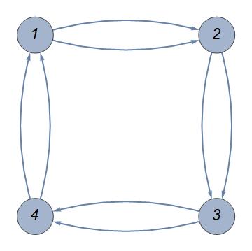
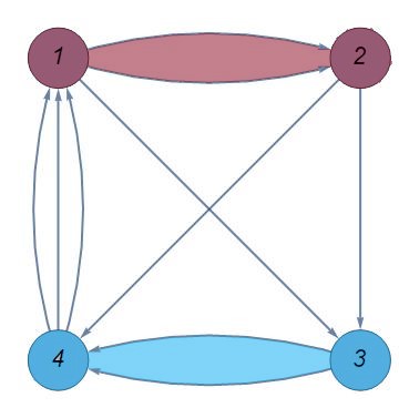
As an example, Closset and Del Zotto argued that the spectrum for local 𝔽0subscript𝔽0\mathbb{F}_{0}, engineering pure SU(2)𝑆𝑈2SU(2) SYM𝑆𝑌𝑀SYM on 4×S1superscript4superscript𝑆1\mathbb{R}^{4}\times S^{1} with Chern-Simons level k=0𝑘0k=0, in such a tame chamber is organised as two copies of the weakly coupled chamber of the four-dimensional pure SU(2)𝑆𝑈2SU(2) gauge theory. The relevant quiver is depicted in Fig.2, and its a adjacency matrix is

B=(0202202002022020).𝐵0202202002022020B=\left(\begin{array}[]{cccc}0&2&0&-2\\ -2&0&2&0\\ 0&-2&0&2\\ 2&0&-2&0\end{array}\right). (4)
Refer to caption
Figure 2: Quiver associated to local 𝔽0subscript𝔽0\mathbb{F}_{0}

The spectrum of this theory was originally derived by using the mutation algorithm in Closset:2019juk . This has been done by using the sequence of mutations

m=μ2μ4μ3μ1,msubscript𝜇2subscript𝜇4subscript𝜇3subscript𝜇1\textbf{m}=\mu_{2}\mu_{4}\mu_{3}\mu_{1}, (5)

which represents the wall-crossing arising from clockwise rotations in the upper half-plane of central charges. The n-th iteration of this operator has the following effect on the charges γisubscript𝛾𝑖\gamma_{i}, i=1,,4𝑖14i=1,\dots,4 of the BPS states:

mn(γ1)=γ1+2nδu,superscriptm𝑛subscript𝛾1subscript𝛾12𝑛subscript𝛿𝑢\displaystyle\textbf{m}^{n}(\gamma_{1})=\gamma_{1}+2n\delta_{u}, mn(γ2)=γ22nδu,superscriptm𝑛subscript𝛾2subscript𝛾22𝑛subscript𝛿𝑢\displaystyle\textbf{m}^{n}(\gamma_{2})=\gamma_{2}-2n\delta_{u}, (6)
mn(γ3)=γ3+2nδd,superscriptm𝑛subscript𝛾3subscript𝛾32𝑛subscript𝛿𝑑\displaystyle\textbf{m}^{n}(\gamma_{3})=\gamma_{3}+2n\delta_{d}, mn(γ4)=γ42nδd,superscriptm𝑛subscript𝛾4subscript𝛾42𝑛subscript𝛿𝑑\displaystyle\textbf{m}^{n}(\gamma_{4})=\gamma_{4}-2n\delta_{d}, (7)

with

δu=γ1+γ2,subscript𝛿𝑢subscript𝛾1subscript𝛾2\displaystyle\delta_{u}=\gamma_{1}+\gamma_{2}, δd=γ3+γ4.subscript𝛿𝑑subscript𝛾3subscript𝛾4\displaystyle\delta_{d}=\gamma_{3}+\gamma_{4}. (8)

The action of m corresponds to rotating out of the upper-half plane the BPS charges in the order 134213421342. The towers of states obtained in this way accumulate on the vector multiplets from one side only. Because of this, the operator m is not sufficient: in order to construct the full spectrum in this chamber, it is necessary to use also the second operator

m^=μ^1μ^3μ^2μ^4,^msubscript^𝜇1subscript^𝜇3subscript^𝜇2subscript^𝜇4\hat{\textbf{m}}=\hat{\mu}_{1}\hat{\mu}_{3}\hat{\mu}_{2}\hat{\mu}_{4}, (9)

constructed from right mutations (3). The shifts obtained from this operator are

m^n(γ1)=γ12nδu,superscript^m𝑛subscript𝛾1subscript𝛾12𝑛subscript𝛿𝑢\displaystyle\hat{\textbf{m}}^{n}(\gamma_{1})=\gamma_{1}-2n\delta_{u}, m^n(γ2)=γ2+2nδu,superscript^m𝑛subscript𝛾2subscript𝛾22𝑛subscript𝛿𝑢\displaystyle\hat{\textbf{m}}^{n}(\gamma_{2})=\gamma_{2}+2n\delta_{u}, (10)
m^n(γ3)=γ32nδd,superscript^m𝑛subscript𝛾3subscript𝛾32𝑛subscript𝛿𝑑\displaystyle\hat{\textbf{m}}^{n}(\gamma_{3})=\gamma_{3}-2n\delta_{d}, m^n(γ4)=γ4+2nδd.superscript^m𝑛subscript𝛾4subscript𝛾42𝑛subscript𝛿𝑑\displaystyle\hat{\textbf{m}}^{n}(\gamma_{4})=\gamma_{4}+2n\delta_{d}. (11)

The resulting BPS spectrum consists of two vector multiplets δu,δdsubscript𝛿𝑢subscript𝛿𝑑\delta_{u},\delta_{d}, and two towers of hypermultiplets

γ1+nδu,subscript𝛾1𝑛subscript𝛿𝑢\displaystyle\gamma_{1}+n\delta_{u}, γ2+nδu,subscript𝛾2𝑛subscript𝛿𝑢\displaystyle\gamma_{2}+n\delta_{u}, γ3+nδd,subscript𝛾3𝑛subscript𝛿𝑑\displaystyle\gamma_{3}+n\delta_{d}, γ4+nδd.subscript𝛾4𝑛subscript𝛿𝑑\displaystyle\gamma_{4}+n\delta_{d}. (12)

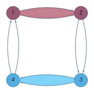
These are two copies of the weakly coupled spectrum of four-dimensional 𝒩=2𝒩2\mathcal{N}=2 SU(2)𝑆𝑈2SU(2) pure SYM, which can be thought as being associated to the decomposition of the quiver 2 into two four-dimensional Krönecker subquivers, as depicted in Figure 3(a).

Let us show an alternative derivation of the above result, making use of the group 𝒢Qsubscript𝒢𝑄\mathcal{G}_{Q} of quiver automorphisms. This contains the semidirect product Dih4W(A1(1))left-normal-factor-semidirect-product𝐷𝑖subscript4𝑊superscriptsubscript𝐴11Dih_{4}\ltimes W(A_{1}^{(1)}), where Dih4𝐷𝑖subscript4Dih_{4} is the dihedral group of the square, which consists only of permutations. The automorphisms group is generated by

π1=(1,3)ι,subscript𝜋113𝜄\displaystyle\pi_{1}=(1,3)\iota, π2=(4,3,2,1),subscript𝜋24321\displaystyle\pi_{2}=(4,3,2,1), T𝔽0=(1,2)(3,4)μ1μ3.subscript𝑇subscript𝔽01234subscript𝜇1subscript𝜇3\displaystyle T_{\mathbb{F}_{0}}=(1,2)(3,4)\mu_{1}\mu_{3}. (13)

The operator T𝔽0subscript𝑇subscript𝔽0T_{\mathbb{F}_{0}} is a Weyl translation on the A1(1)superscriptsubscript𝐴11A_{1}^{(1)} lattice.

Refer to caption
(a) Subquiver decomposition for T𝔽0subscript𝑇subscript𝔽0T_{\mathbb{F}_{0}}
Refer to caption
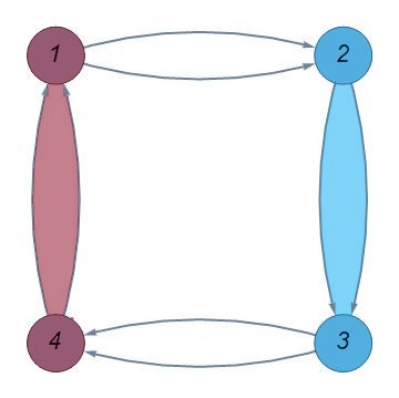
(b) Subquiver decomposition for T𝔽0subscriptsuperscript𝑇subscript𝔽0T^{\prime}_{\mathbb{F}_{0}}
Figure 3:

This operator directly generates the whole BPS spectrum of the theory by acting on the charges. Indeed, by applying the mutation rules (2) we obtain

T𝔽0n(γ1)=γ1+nδu,subscriptsuperscript𝑇𝑛subscript𝔽0subscript𝛾1subscript𝛾1𝑛subscript𝛿𝑢\displaystyle T^{n}_{\mathbb{F}_{0}}(\gamma_{1})=\gamma_{1}+n\delta_{u}, T𝔽0n(γ2)=γ2nδu,subscriptsuperscript𝑇𝑛subscript𝔽0subscript𝛾2subscript𝛾2𝑛subscript𝛿𝑢\displaystyle T^{n}_{\mathbb{F}_{0}}(\gamma_{2})=\gamma_{2}-n\delta_{u}, (14)
T𝔽0n(γ3)=γ3+nδdsubscriptsuperscript𝑇𝑛subscript𝔽0subscript𝛾3subscript𝛾3𝑛subscript𝛿𝑑\displaystyle T^{n}_{\mathbb{F}_{0}}(\gamma_{3})=\gamma_{3}+n\delta_{d} T𝔽0n(γ4)=γ4nδd.subscriptsuperscript𝑇𝑛subscript𝔽0subscript𝛾4subscript𝛾4𝑛subscript𝛿𝑑\displaystyle T^{n}_{\mathbb{F}_{0}}(\gamma_{4})=\gamma_{4}-n\delta_{d}. (15)

By computing the Dirac pairing of these states, which is given by the adjacency matrix of the quiver, in particular

δu,δd=δuTBδd=0,subscript𝛿𝑢subscript𝛿𝑑superscriptsubscript𝛿𝑢𝑇𝐵subscript𝛿𝑑0\langle\delta_{u},\delta_{d}\rangle=\delta_{u}^{T}\cdot B\cdot\delta_{d}=0, (16)

we see that T𝔽0subscript𝑇subscript𝔽0T_{\mathbb{F}_{0}} generates mutually local towers of states

γ1+nδu,subscript𝛾1𝑛subscript𝛿𝑢\displaystyle\gamma_{1}+n\delta_{u}, γ4+nδd,subscript𝛾4𝑛subscript𝛿𝑑\displaystyle\gamma_{4}+n\delta_{d}, (17)

and

γ2+nδu,subscript𝛾2𝑛subscript𝛿𝑢\displaystyle\gamma_{2}+n\delta_{u}, γ3+nδd.subscript𝛾3𝑛subscript𝛿𝑑\displaystyle\gamma_{3}+n\delta_{d}. (18)

As n𝑛n\rightarrow\infty, the towers of states accumulate to the vectors δu,δdsubscript𝛿𝑢subscript𝛿𝑑\delta_{u},\delta_{d}, which are vector multiplets for the four-dimensional quivers that decompose the five-dimensional quiver as in Figure 3(a). The mutation operators m,m^m^m\textbf{m},\hat{\textbf{m}} are related in a simple way to the the time evolution operator:

m=T𝔽02,msuperscriptsubscript𝑇subscript𝔽02\displaystyle\textbf{m}=T_{\mathbb{F}_{0}}^{2}, m^=T𝔽02ι,^msuperscriptsubscript𝑇subscript𝔽02𝜄\displaystyle\hat{\textbf{m}}=T_{\mathbb{F}_{0}}^{-2}\iota, (19)

where ι𝜄\iota is the inversion. From the perspective of the full automorphism group

W~(A1(1))Dih4,left-normal-factor-semidirect-product~𝑊superscriptsubscript𝐴11𝐷𝑖subscript4\widetilde{W}(A_{1}^{(1)})\ltimes Dih_{4}, (20)

it is natural to consider also another translation operator

T𝔽0=(2,3)(1,4)μ2μ4,subscriptsuperscript𝑇subscript𝔽02314subscript𝜇2subscript𝜇4T^{\prime}_{\mathbb{F}_{0}}=(2,3)(1,4)\mu_{2}\mu_{4}, (21)

whose action on the charges is

(T𝔽0)n(γ1)=γ1n(γ1+γ4),superscriptsubscriptsuperscript𝑇subscript𝔽0𝑛subscript𝛾1subscript𝛾1𝑛subscript𝛾1subscript𝛾4\displaystyle\left(T^{\prime}_{\mathbb{F}_{0}}\right)^{n}(\gamma_{1})=\gamma_{1}-n(\gamma_{1}+\gamma_{4}), (T𝔽0)n(γ2)=γ2+n(γ2+γ3),superscriptsubscriptsuperscript𝑇subscript𝔽0𝑛subscript𝛾2subscript𝛾2𝑛subscript𝛾2subscript𝛾3\displaystyle\left(T^{\prime}_{\mathbb{F}_{0}}\right)^{n}(\gamma_{2})=\gamma_{2}+n(\gamma_{2}+\gamma_{3}), (22)
(T𝔽0)n(γ3)=γ3n(γ2+γ3),superscriptsubscriptsuperscript𝑇subscript𝔽0𝑛subscript𝛾3subscript𝛾3𝑛subscript𝛾2subscript𝛾3\displaystyle\left(T^{\prime}_{\mathbb{F}_{0}}\right)^{n}(\gamma_{3})=\gamma_{3}-n(\gamma_{2}+\gamma_{3}), (T𝔽0)n(γ4)=γ4+n(γ1+γ4).superscriptsubscriptsuperscript𝑇subscript𝔽0𝑛subscript𝛾4subscript𝛾4𝑛subscript𝛾1subscript𝛾4\displaystyle\left(T^{\prime}_{\mathbb{F}_{0}}\right)^{n}(\gamma_{4})=\gamma_{4}+n(\gamma_{1}+\gamma_{4}). (23)

This generates different towers of hypermultiplets, which are still organized as two copies of the weakly coupled chamber of four-dimensional super Yang-Mills, with vector multiplets

δl=γ1+γ4,subscript𝛿𝑙subscript𝛾1subscript𝛾4\displaystyle\delta_{l}=\gamma_{1}+\gamma_{4}, δr=γ2+γ3.subscript𝛿𝑟subscript𝛾2subscript𝛾3\displaystyle\delta_{r}=\gamma_{2}+\gamma_{3}. (24)

In this way, we find a different infinite chamber, corresponding to the decomposition of the 5d BPS quiver as in Figure 3(b).

We see that considering the natural translation operators associated to the quiver automorphisms builds the correct spectrum for the tame chambers in a simpler way, without the need to consider both left and right mutations. This simplification occurs because we are allowing not just mutations, but also permutations, which are relabelings of the BPS charges. This operation of course has no effect on the resulting spectrum, which is the same as the one emerging from using just the mutation algorithm. However, by using quiver automorphisms, it is possible to construct more elementary dualities of the theory, and the spectrum can be constructed more simply. This plays a crucial rôle in more complicated cases. To illustrate this point we discuss in the following the cases of local 𝔽1subscript𝔽1\mathbb{F}_{1} and dP3subscriptdP3\text{dP}_{3}.

2.2 Super Yang-Mills, k=1𝑘1k=1

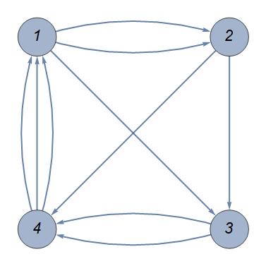
The local 𝔽1subscript𝔽1\mathbb{F}_{1} quiver is displayed in Figure 4(a). This engineers pure SU(2)𝑆𝑈2SU(2) SYM with 5d Chern-Simons level k=1𝑘1k=1. The adjacency matrix is

B=(0213201111023120).𝐵0213201111023120B=\left(\begin{array}[]{cccc}0&2&1&-3\\ -2&0&1&1\\ -1&-1&0&2\\ 3&-1&-2&0\end{array}\right). (25)

The traslation operator is given by

T𝔽1=(1324)μ3.subscript𝑇subscript𝔽11324subscript𝜇3T_{\mathbb{F}_{1}}=(1324)\mu_{3}. (26)
Refer to caption
(a) Quiver associated to local 𝔽1subscript𝔽1\mathbb{F}_{1}
Refer to caption
(b) 4d subquivers for local 𝔽1subscript𝔽1\mathbb{F}_{1}
Figure 4:

As far as the spectrum is concerned, this is the same as the local 𝔽0subscript𝔽0\mathbb{F}_{0} one. The operators m,m~m~m\textbf{m},\tilde{\textbf{m}} are easy to build

mT𝔽14=((1324)μ3)4,msuperscriptsubscript𝑇subscript𝔽14superscript1324subscript𝜇34\displaystyle\textbf{m}\equiv T_{\mathbb{F}_{1}}^{4}=\left((1324)\mu_{3}\right)^{4}, m^T𝔽14ι.^msuperscriptsubscript𝑇subscript𝔽14𝜄\displaystyle\hat{\textbf{m}}\equiv T_{\mathbb{F}_{1}}^{-4}\iota. (27)

and the associated evolution on the vector of charges 𝜸𝜸\boldsymbol{\gamma} is

T𝔽12n(𝜸)=T𝔽0n(𝜸)=(γ1+nδuγ2nδuγ3+nδdγ4nδd),superscriptsubscript𝑇subscript𝔽12𝑛𝜸superscriptsubscript𝑇subscript𝔽0𝑛𝜸subscript𝛾1𝑛subscript𝛿𝑢subscript𝛾2𝑛subscript𝛿𝑢subscript𝛾3𝑛subscript𝛿𝑑subscript𝛾4𝑛subscript𝛿𝑑T_{\mathbb{F}_{1}}^{2n}(\boldsymbol{\gamma})=T_{\mathbb{F}_{0}}^{n}(\boldsymbol{\gamma})=\left(\begin{array}[]{cccc}\gamma_{1}+n\delta_{u}&\gamma_{2}-n\delta_{u}&\gamma_{3}+n\delta_{d}&\gamma_{4}-n\delta_{d}\end{array}\right), (28)
T𝔽12n1(𝜸)=(γ3+nδd,γ4nδd,γ2nδu,γ1+nδu,).superscriptsubscript𝑇subscript𝔽12𝑛1𝜸subscript𝛾3𝑛subscript𝛿𝑑subscript𝛾4𝑛subscript𝛿𝑑subscript𝛾2𝑛subscript𝛿𝑢subscript𝛾1𝑛subscript𝛿𝑢T_{\mathbb{F}_{1}}^{2n-1}(\boldsymbol{\gamma})=\left(\begin{array}[]{cccc}\gamma_{3}+n\delta_{d},&\gamma_{4}-n\delta_{d},&\gamma_{2}-n\delta_{u},&\gamma_{1}+n\delta_{u},\end{array}\right). (29)

We see that even though the introduction of a Chern-Simons level will affect some physical aspects, it does not modify the type of states in the spectrum: again δu,δdsubscript𝛿𝑢subscript𝛿𝑑\delta_{u},\delta_{d} correspond to the vector multiplets of the 4d subquivers depicted in Figure 4(b). What changes however is the number of tame chambers: because the symmetry group now does not include the Dih4𝐷𝑖subscript4Dih_{4} factor – as it is clear by inspection of the quiver – there is not the related chamber.

2.3 Nf=2subscript𝑁𝑓2N_{f}=2, k=0𝑘0k=0

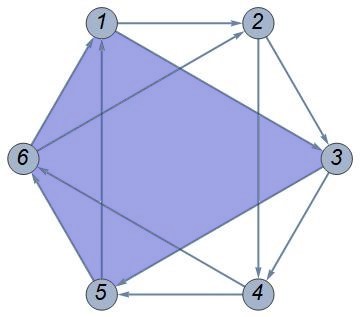
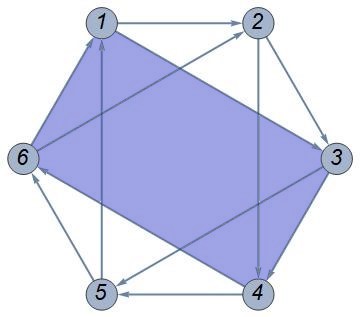
Refer to caption
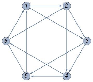
Figure 5: Quiver for dP3subscriptdP3\text{dP}_{3}

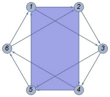
When we include matter the situation is much richer, because we encounter the new feature of multiple commuting flows, each characterizing the spectrum in a different chamber of the moduli space. The relevant quiver is the one of dP3𝑑subscript𝑃3dP_{3}, engineering the SU(2)𝑆𝑈2SU(2) theory with two flavors, depicted in Figure 10. It has adjacency matrix

B=(011011101101110110011011101101110110).𝐵011011101101110110011011101101110110B=\left(\begin{array}[]{cccccc}0&1&1&0&-1&-1\\ -1&0&1&1&0&-1\\ -1&-1&0&1&1&0\\ 0&-1&-1&0&1&1\\ 1&0&-1&-1&0&1\\ 1&1&0&-1&-1&0\end{array}\right). (30)

The extended Weyl group is W~((A2+A1)(1))~𝑊superscriptsubscript𝐴2subscript𝐴11\tilde{W}((A_{2}+A_{1})^{(1)}), which is generated by

s0=(3,6)μ6μ3subscript𝑠036subscript𝜇6subscript𝜇3\displaystyle s_{0}=(3,6)\mu_{6}\mu_{3} s1=(1,4)μ4μ1,subscript𝑠114subscript𝜇4subscript𝜇1\displaystyle s_{1}=(1,4)\mu_{4}\mu_{1}, s2=(2,5)μ5μ2,subscript𝑠225subscript𝜇5subscript𝜇2\displaystyle s_{2}=(2,5)\mu_{5}\mu_{2}, (31)
r0=(4,6)μ2μ4μ6μ2,subscript𝑟046subscript𝜇2subscript𝜇4subscript𝜇6subscript𝜇2\displaystyle r_{0}=(4,6)\mu_{2}\mu_{4}\mu_{6}\mu_{2}, r1=(3,5)μ1μ3μ5μ1,subscript𝑟135subscript𝜇1subscript𝜇3subscript𝜇5subscript𝜇1\displaystyle r_{1}=(3,5)\mu_{1}\mu_{3}\mu_{5}\mu_{1}, (32)
π=(1,2,3,4,5,6),𝜋123456\displaystyle\pi=(1,2,3,4,5,6), σ=(1,4)(2,3)(5,6)ι.𝜎142356𝜄\displaystyle\sigma=(1,4)(2,3)(5,6)\iota. (33)

In this case there are four commuting evolution operators, given by Weyl translations of W~((A2+A1)(1))~𝑊superscriptsubscript𝐴2subscript𝐴11\tilde{W}((A_{2}+A_{1})^{(1)}), acting on the affine root lattice Q((A2+A1)(1))𝑄superscriptsubscript𝐴2subscript𝐴11Q\left((A_{2}+A_{1})^{(1)}\right) 2006LMaPh..75…39T ; doi:10.1063/1.4931481 222For the action on the roots, see Section 3.3.. One has the three operators

T1=s0s2π,subscript𝑇1subscript𝑠0subscript𝑠2𝜋\displaystyle T_{1}=s_{0}s_{2}\pi, T2=s1s0π,subscript𝑇2subscript𝑠1subscript𝑠0𝜋\displaystyle T_{2}=s_{1}s_{0}\pi, T3=s2s1πsubscript𝑇3subscript𝑠2subscript𝑠1𝜋\displaystyle T_{3}=s_{2}s_{1}\pi (34)

satisfying T1T2T3=1subscript𝑇1subscript𝑇2subscript𝑇31T_{1}T_{2}T_{3}=1, and finally

T4=r0π3.subscript𝑇4subscript𝑟0superscript𝜋3T_{4}=r_{0}\pi^{3}\,. (35)
Refer to caption
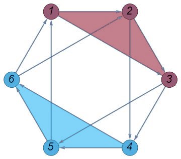
Figure 6: 4d subquivers for local dP3𝑑subscript𝑃3dP_{3}, under T1subscript𝑇1T_{1}

Let us consider the flow T1subscript𝑇1T_{1} first, given by

T1=s0s2π=(3,6)μ6μ3(2,5)μ5μ2(1,2,3,4,5,6).subscript𝑇1subscript𝑠0subscript𝑠2𝜋36subscript𝜇6subscript𝜇325subscript𝜇5subscript𝜇2123456T_{1}=s_{0}s_{2}\pi=(3,6)\mu_{6}\mu_{3}(2,5)\mu_{5}\mu_{2}(1,2,3,4,5,6). (36)

Its action on the BPS charges is the following:

T1n:(γ1γ2γ3γ4γ5γ6)((n+1)γ1+n(γ2+γ3),γ2,(n+1)(γ1+γ2)nγ3,γ4+n(γ4+γ5+γ6),γ5,(n+1)(γ4+γ5)nγ6):superscriptsubscript𝑇1𝑛subscript𝛾1subscript𝛾2subscript𝛾3subscript𝛾4subscript𝛾5subscript𝛾6𝑛1subscript𝛾1𝑛subscript𝛾2subscript𝛾3subscript𝛾2𝑛1subscript𝛾1subscript𝛾2𝑛subscript𝛾3subscript𝛾4𝑛subscript𝛾4subscript𝛾5subscript𝛾6subscript𝛾5𝑛1subscript𝛾4subscript𝛾5𝑛subscript𝛾6T_{1}^{n}:\left(\begin{array}[]{c}\gamma_{1}\\ \gamma_{2}\\ \gamma_{3}\\ \gamma_{4}\\ \gamma_{5}\\ \gamma_{6}\end{array}\right)\longrightarrow\left(\begin{array}[]{c}(n+1)\gamma_{1}+n(\gamma_{2}+\gamma_{3}),\\ \gamma_{2},\\ -(n+1)(\gamma_{1}+\gamma_{2})-n\gamma_{3},\\ \gamma_{4}+n(\gamma_{4}+\gamma_{5}+\gamma_{6}),\\ \gamma_{5},\\ -(n+1)(\gamma_{4}+\gamma_{5})-n\gamma_{6}\end{array}\right) (37)

We see that T1subscript𝑇1T_{1} generates infinite towers of hypermultiplets given by

γ1+n(γ1+γ2+γ3),subscript𝛾1𝑛subscript𝛾1subscript𝛾2subscript𝛾3\displaystyle\gamma_{1}+n(\gamma_{1}+\gamma_{2}+\gamma_{3}), (n+1)(γ1+γ2)nγ3,𝑛1subscript𝛾1subscript𝛾2𝑛subscript𝛾3\displaystyle-(n+1)(\gamma_{1}+\gamma_{2})-n\gamma_{3}, (38)
γ4+n(γ4+γ5+γ6),subscript𝛾4𝑛subscript𝛾4subscript𝛾5subscript𝛾6\displaystyle\gamma_{4}+n(\gamma_{4}+\gamma_{5}+\gamma_{6}), (n+1)(γ4+γ5)nγ6.𝑛1subscript𝛾4subscript𝛾5𝑛subscript𝛾6\displaystyle-(n+1)(\gamma_{4}+\gamma_{5})-n\gamma_{6}. (39)

These are the BPS states corresponding to two copies of the weakly-coupled spectrum for the Nf=1subscript𝑁𝑓1N_{f}=1 theory in four dimensions, and correspond to the decomposition of the 5d quiver into two 4d subquivers for Nf=1subscript𝑁𝑓1N_{f}=1, as in Figure 6. One can easily check that the towers of states are mutually local, and as n𝑛n\rightarrow\infty they accumulate on the rays

δu(1)=γ1+γ2+γ3,superscriptsubscript𝛿𝑢1subscript𝛾1subscript𝛾2subscript𝛾3\displaystyle\delta_{u}^{(1)}=\gamma_{1}+\gamma_{2}+\gamma_{3}, δd(1)=γ4+γ5+γ6,superscriptsubscript𝛿𝑑1subscript𝛾4subscript𝛾5subscript𝛾6\displaystyle\delta_{d}^{(1)}=\gamma_{4}+\gamma_{5}+\gamma_{6}, (40)

which are indeed the vector multiplets for the 4d Nf=1subscript𝑁𝑓1N_{f}=1 subquivers. More precisely, the towers of hypermultiplets above are only half of the towers from Nf=1subscript𝑁𝑓1N_{f}=1 theory. To complete the picture here we have to consider, like in the pure gauge case, the states constructed from right mutations: these are generated as before by powers of the inverse of the evolution operator, composed with an inversion ι𝜄\iota:

T1nι:(γ1γ2γ3γ4γ5γ6)(nγ1(n+1)(γ2+γ3)γ2nγ3+(n+1)(γ1+γ2)nγ4(n+1)(γ5+γ6)γ5(n+1)γ6+n(γ5+γ4).):superscriptsubscript𝑇1𝑛𝜄subscript𝛾1subscript𝛾2subscript𝛾3subscript𝛾4subscript𝛾5subscript𝛾6𝑛subscript𝛾1𝑛1subscript𝛾2subscript𝛾3subscript𝛾2𝑛subscript𝛾3𝑛1subscript𝛾1subscript𝛾2𝑛subscript𝛾4𝑛1subscript𝛾5subscript𝛾6subscript𝛾5𝑛1subscript𝛾6𝑛subscript𝛾5subscript𝛾4T_{1}^{-n}\iota:\left(\begin{array}[]{c}\gamma_{1}\\ \gamma_{2}\\ \gamma_{3}\\ \gamma_{4}\\ \gamma_{5}\\ \gamma_{6}\end{array}\right)\longrightarrow\left(\begin{array}[]{c}-n\gamma_{1}-(n+1)(\gamma_{2}+\gamma_{3})\\ \gamma_{2}\\ n\gamma_{3}+(n+1)(\gamma_{1}+\gamma_{2})\\ -n\gamma_{4}-(n+1)(\gamma_{5}+\gamma_{6})\\ \gamma_{5}\\ (n+1)\gamma_{6}+n(\gamma_{5}+\gamma_{4}).\end{array}\right) (41)

The spectrum of the Nf=1subscript𝑁𝑓1N_{f}=1 theory in four dimensions also includes two quarks, that for the subquivers in Figure 6 are given by γ5,γ4+γ6,γ2,γ1+γ3subscript𝛾5subscript𝛾4subscript𝛾6subscript𝛾2subscript𝛾1subscript𝛾3\gamma_{5},\gamma_{4}+\gamma_{6},\gamma_{2},\gamma_{1}+\gamma_{3}. We see that we recover the quarks γ5,γ2subscript𝛾5subscript𝛾2\gamma_{5},\gamma_{2} as the states that are left invariant by T1subscript𝑇1T_{1}, while the other quarks would be their complementary in the subquiver. We will see below how the remaining quarks can be recovered as the states that are fixed by a different flow.
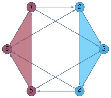
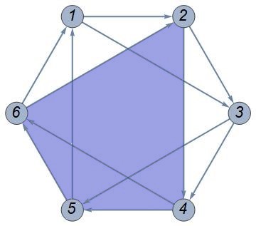
Refer to caption
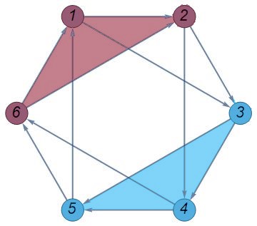
Figure 7: 4d subquivers for local dP3𝑑subscript𝑃3dP_{3}, under T2subscript𝑇2T_{2}

T2subscript𝑇2T_{2} is given by

T2=s1s0π=(1,4)μ4μ1(3,6)μ6μ3(1,2,3,4,5,6),subscript𝑇2subscript𝑠1subscript𝑠0𝜋14subscript𝜇4subscript𝜇136subscript𝜇6subscript𝜇3123456T_{2}=s_{1}s_{0}\pi=(1,4)\mu_{4}\mu_{1}(3,6)\mu_{6}\mu_{3}(1,2,3,4,5,6), (42)

and acts on the BPS charges as

T2n:(γ1γ2γ3γ4γ5γ6)(nγ1(n+1)(γ5+γ6)(n+1)γ2+n(γ3+γ4)γ3n(γ2+γ3)nγ4(n+1)γ5+n(γ1+γ6)γ6.):superscriptsubscript𝑇2𝑛subscript𝛾1subscript𝛾2subscript𝛾3subscript𝛾4subscript𝛾5subscript𝛾6𝑛subscript𝛾1𝑛1subscript𝛾5subscript𝛾6𝑛1subscript𝛾2𝑛subscript𝛾3subscript𝛾4subscript𝛾3𝑛subscript𝛾2subscript𝛾3𝑛subscript𝛾4𝑛1subscript𝛾5𝑛subscript𝛾1subscript𝛾6subscript𝛾6T_{2}^{n}:\left(\begin{array}[]{c}\gamma_{1}\\ \gamma_{2}\\ \gamma_{3}\\ \gamma_{4}\\ \gamma_{5}\\ \gamma_{6}\end{array}\right)\longrightarrow\left(\begin{array}[]{c}-n\gamma_{1}-(n+1)(\gamma_{5}+\gamma_{6})\\ (n+1)\gamma_{2}+n(\gamma_{3}+\gamma_{4})\\ \gamma_{3}\\ -n(\gamma_{2}+\gamma_{3})-n\gamma_{4}\\ (n+1)\gamma_{5}+n(\gamma_{1}+\gamma_{6})\\ \gamma_{6}.\end{array}\right) (43)

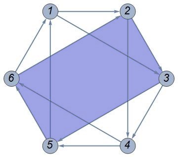
Reasoning as before, we find that the spectrum in this chamber is organized in two copies of the 4d Nf=1subscript𝑁𝑓1N_{f}=1 weakly coupled chamber, corresponding to the subquiver decomposition in Figure 7, with vector multiplets

δ2(u)=γ1+γ5+γ6,superscriptsubscript𝛿2𝑢subscript𝛾1subscript𝛾5subscript𝛾6\displaystyle\delta_{2}^{(u)}=\gamma_{1}+\gamma_{5}+\gamma_{6}, δ2(d)=γ2+γ3+γ4.superscriptsubscript𝛿2𝑑subscript𝛾2subscript𝛾3subscript𝛾4\displaystyle\delta_{2}^{(d)}=\gamma_{2}+\gamma_{3}+\gamma_{4}. (44)

Finally, we have

T3=s2s1π=(2,5)μ5μ2(1,4)μ4μ1(1,2,3,4,5,6),subscript𝑇3subscript𝑠2subscript𝑠1𝜋25subscript𝜇5subscript𝜇214subscript𝜇4subscript𝜇1123456T_{3}=s_{2}s_{1}\pi=(2,5)\mu_{5}\mu_{2}(1,4)\mu_{4}\mu_{1}(1,2,3,4,5,6), (45)

with action

T3n:(γ1γ2γ3γ4γ5γ6)(γ1nγ2(n+1)(γ1+γ6)(n+1)γ3+n(γ4+γ5)γ4nγ5(n+1)(γ3+γ4)(n+1)γ6+n(γ1+γ2)),:superscriptsubscript𝑇3𝑛subscript𝛾1subscript𝛾2subscript𝛾3subscript𝛾4subscript𝛾5subscript𝛾6subscript𝛾1𝑛subscript𝛾2𝑛1subscript𝛾1subscript𝛾6𝑛1subscript𝛾3𝑛subscript𝛾4subscript𝛾5subscript𝛾4𝑛subscript𝛾5𝑛1subscript𝛾3subscript𝛾4𝑛1subscript𝛾6𝑛subscript𝛾1subscript𝛾2T_{3}^{n}:\left(\begin{array}[]{c}\gamma_{1}\\ \gamma_{2}\\ \gamma_{3}\\ \gamma_{4}\\ \gamma_{5}\\ \gamma_{6}\end{array}\right)\longrightarrow\left(\begin{array}[]{c}\gamma_{1}\\ -n\gamma_{2}-(n+1)(\gamma_{1}+\gamma_{6})\\ (n+1)\gamma_{3}+n(\gamma_{4}+\gamma_{5})\\ \gamma_{4}\\ -n\gamma_{5}-(n+1)(\gamma_{3}+\gamma_{4})\\ (n+1)\gamma_{6}+n(\gamma_{1}+\gamma_{2})\end{array}\right), (46)

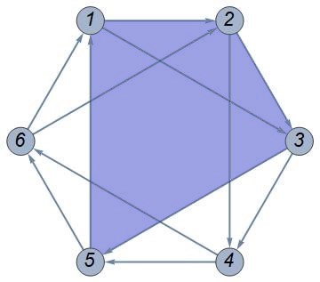
which gives another chamber organized as two copies of four-dimensional weakly coupled Nf=1subscript𝑁𝑓1N_{f}=1 depicted in Figure 8, with vector multiplets

δ3(u)=γ1+γ2+γ6,superscriptsubscript𝛿3𝑢subscript𝛾1subscript𝛾2subscript𝛾6\displaystyle\delta_{3}^{(u)}=\gamma_{1}+\gamma_{2}+\gamma_{6}, δ3(d)=γ3+γ4+γ5.superscriptsubscript𝛿3𝑑subscript𝛾3subscript𝛾4subscript𝛾5\displaystyle\delta_{3}^{(d)}=\gamma_{3}+\gamma_{4}+\gamma_{5}. (47)

Before considering the evolution T4subscript𝑇4T_{4}, let us make a remark. The picture above suggests that there exists a relation between the different flows in terms of permutations of the nodes of the quiver. Indeed, it is possible to check that we have the relations

T1=(3,4,5,6,1,2)T2(5,6,1,2,3,4)=(6,1,2,3,4,5)T3(2,3,4,5,6,1).subscript𝑇1345612subscript𝑇2561234612345subscript𝑇3234561T_{1}=(3,4,5,6,1,2)T_{2}(5,6,1,2,3,4)=(6,1,2,3,4,5)T_{3}(2,3,4,5,6,1)\,. (48)
Refer to caption
Figure 8: 4d subquivers for local dP3𝑑subscript𝑃3dP_{3}, under T3subscript𝑇3T_{3}

From the point of view of the BPS spectrum, it is now clear that these three flows will generate the same spectrum up to relabeling of states, i.e. they will differ in what we call electric or magnetic in the field theory. Another interesting quiver automorphism is given by

R2=π2s1=(3,5,1)(4,2,6)(1,4)μ4μ1,subscript𝑅2superscript𝜋2subscript𝑠135142614subscript𝜇4subscript𝜇1R_{2}=\pi^{2}s_{1}=(3,5,1)(4,2,6)(1,4)\mu_{4}\mu_{1}, (49)

which is known as half-translation, because it satisfies R22=T2superscriptsubscript𝑅22subscript𝑇2R_{2}^{2}=T_{2} (half-translations for T1,T3subscript𝑇1subscript𝑇3T_{1},T_{3} can be obtained by using equation (48)). Under this quiver automorphism, the BPS charges transform as

R22n+1:(γ1γ2γ3γ4γ5γ6)((n+1)γ2n(γ3+γ4)nγ1+(n+1)(γ5+γ6)γ1+γ5(n+1)γ5n(γ1+γ6)nγ4+(n+1)(γ2+γ3)γ2+γ4),:superscriptsubscript𝑅22𝑛1subscript𝛾1subscript𝛾2subscript𝛾3subscript𝛾4subscript𝛾5subscript𝛾6𝑛1subscript𝛾2𝑛subscript𝛾3subscript𝛾4𝑛subscript𝛾1𝑛1subscript𝛾5subscript𝛾6subscript𝛾1subscript𝛾5𝑛1subscript𝛾5𝑛subscript𝛾1subscript𝛾6𝑛subscript𝛾4𝑛1subscript𝛾2subscript𝛾3subscript𝛾2subscript𝛾4R_{2}^{2n+1}:\left(\begin{array}[]{c}\gamma_{1}\\ \gamma_{2}\\ \gamma_{3}\\ \gamma_{4}\\ \gamma_{5}\\ \gamma_{6}\end{array}\right)\longrightarrow\left(\begin{array}[]{c}-(n+1)\gamma_{2}-n(\gamma_{3}+\gamma_{4})\\ n\gamma_{1}+(n+1)(\gamma_{5}+\gamma_{6})\\ \gamma_{1}+\gamma_{5}\\ -(n+1)\gamma_{5}-n(\gamma_{1}+\gamma_{6})\\ n\gamma_{4}+(n+1)(\gamma_{2}+\gamma_{3})\\ \gamma_{2}+\gamma_{4}\end{array}\right), (50)

while of course R22n=T2nsuperscriptsubscript𝑅22𝑛superscriptsubscript𝑇2𝑛R_{2}^{2n}=T_{2}^{n}. Note that this generates the CPT conjugates of the towers of states as T2subscript𝑇2T_{2}, while the states that are left fixed by the action of R2subscript𝑅2R_{2} are exactly the missing quarks from our analysis of T2subscript𝑇2T_{2}, so that R2subscript𝑅2R_{2} generates the full spectrum of the two copies of Nf=1subscript𝑁𝑓1N_{f}=1 in the subquivers of Figure 7.

Finally, the time evolution T4subscript𝑇4T_{4} is given by

T4=r0π3=(4,6)μ2μ4μ6μ2(4,5,6,1,2,3),subscript𝑇4subscript𝑟0superscript𝜋346subscript𝜇2subscript𝜇4subscript𝜇6subscript𝜇2456123T_{4}=r_{0}\pi^{3}=(4,6)\mu_{2}\mu_{4}\mu_{6}\mu_{2}(4,5,6,1,2,3), (51)

and acts on the BPS charges as follows:

T43n2:(γ1γ2γ3γ4γ5γ6)(γ1+(γ3+γ4)+nδγ2(γ1+γ2)nδγ3+(γ5+γ6)+nδγ4(γ3+γ4)nδγ5+(γ1+γ2)+nδγ6(γ5+γ6)nδ),:superscriptsubscript𝑇43𝑛2subscript𝛾1subscript𝛾2subscript𝛾3subscript𝛾4subscript𝛾5subscript𝛾6subscript𝛾1subscript𝛾3subscript𝛾4𝑛𝛿subscript𝛾2subscript𝛾1subscript𝛾2𝑛𝛿subscript𝛾3subscript𝛾5subscript𝛾6𝑛𝛿subscript𝛾4subscript𝛾3subscript𝛾4𝑛𝛿subscript𝛾5subscript𝛾1subscript𝛾2𝑛𝛿subscript𝛾6subscript𝛾5subscript𝛾6𝑛𝛿T_{4}^{3n-2}:\left(\begin{array}[]{c}\gamma_{1}\\ \gamma_{2}\\ \gamma_{3}\\ \gamma_{4}\\ \gamma_{5}\\ \gamma_{6}\end{array}\right)\longrightarrow\left(\begin{array}[]{c}\gamma_{1}+(\gamma_{3}+\gamma_{4})+n\delta\\ \gamma_{2}-(\gamma_{1}+\gamma_{2})-n\delta\\ \gamma_{3}+(\gamma_{5}+\gamma_{6})+n\delta\\ \gamma_{4}-(\gamma_{3}+\gamma_{4})-n\delta\\ \gamma_{5}+(\gamma_{1}+\gamma_{2})+n\delta\\ \gamma_{6}-(\gamma_{5}+\gamma_{6})-n\delta\end{array}\right), (52)
T43n1:(γ1γ2γ3γ4γ5γ6)(γ1+(γ3+γ4+γ5+γ6)+nδγ2(γ1+γ2+γ3+γ4)nδγ3+(γ1+γ2+γ5+γ6)+nδγ4(γ3+γ4+γ5+γ6)nδγ5+(γ1+γ2+γ3+γ4)+nδγ6(γ1+γ2+γ5+γ6)nδ),:superscriptsubscript𝑇43𝑛1subscript𝛾1subscript𝛾2subscript𝛾3subscript𝛾4subscript𝛾5subscript𝛾6subscript𝛾1subscript𝛾3subscript𝛾4subscript𝛾5subscript𝛾6𝑛𝛿subscript𝛾2subscript𝛾1subscript𝛾2subscript𝛾3subscript𝛾4𝑛𝛿subscript𝛾3subscript𝛾1subscript𝛾2subscript𝛾5subscript𝛾6𝑛𝛿subscript𝛾4subscript𝛾3subscript𝛾4subscript𝛾5subscript𝛾6𝑛𝛿subscript𝛾5subscript𝛾1subscript𝛾2subscript𝛾3subscript𝛾4𝑛𝛿subscript𝛾6subscript𝛾1subscript𝛾2subscript𝛾5subscript𝛾6𝑛𝛿T_{4}^{3n-1}:\left(\begin{array}[]{c}\gamma_{1}\\ \gamma_{2}\\ \gamma_{3}\\ \gamma_{4}\\ \gamma_{5}\\ \gamma_{6}\end{array}\right)\longrightarrow\left(\begin{array}[]{c}\gamma_{1}+(\gamma_{3}+\gamma_{4}+\gamma_{5}+\gamma_{6})+n\delta\\ \gamma_{2}-(\gamma_{1}+\gamma_{2}+\gamma_{3}+\gamma_{4})-n\delta\\ \gamma_{3}+(\gamma_{1}+\gamma_{2}+\gamma_{5}+\gamma_{6})+n\delta\\ \gamma_{4}-(\gamma_{3}+\gamma_{4}+\gamma_{5}+\gamma_{6})-n\delta\\ \gamma_{5}+(\gamma_{1}+\gamma_{2}+\gamma_{3}+\gamma_{4})+n\delta\\ \gamma_{6}-(\gamma_{1}+\gamma_{2}+\gamma_{5}+\gamma_{6})-n\delta\end{array}\right), (53)
T43n:(γ1γ2γ3γ4γ5γ6)(γ1+nδγ2nδγ3+nδγ4nδγ5+nδγ6nδ).:superscriptsubscript𝑇43𝑛subscript𝛾1subscript𝛾2subscript𝛾3subscript𝛾4subscript𝛾5subscript𝛾6subscript𝛾1𝑛𝛿subscript𝛾2𝑛𝛿subscript𝛾3𝑛𝛿subscript𝛾4𝑛𝛿subscript𝛾5𝑛𝛿subscript𝛾6𝑛𝛿T_{4}^{3n}:\left(\begin{array}[]{c}\gamma_{1}\\ \gamma_{2}\\ \gamma_{3}\\ \gamma_{4}\\ \gamma_{5}\\ \gamma_{6}\end{array}\right)\longrightarrow\left(\begin{array}[]{c}\gamma_{1}+n\delta\\ \gamma_{2}-n\delta\\ \gamma_{3}+n\delta\\ \gamma_{4}-n\delta\\ \gamma_{5}+n\delta\\ \gamma_{6}-n\delta\end{array}\right). (54)

We can recognise in this chamber towers of states that accumulate to the same BPS ray δ=γ1++γ6𝛿subscript𝛾1subscript𝛾6\delta=\gamma_{1}+\dots+\gamma_{6}, representing a multiplet with higher spin s1𝑠1s\geq 1. In this case the four-dimensional interpretation is subtler and more interesting, and we postpone it to Section 5.3.

3 Discrete BPS quiver dynamics, cluster algebras and q-Painlevé equations

The translation operators acting on the BPS quivers we described so far can be regarded as time evolution operators for discrete dynamical systems arising from deautonomization of cluster integrable systems, naturally associated to the geometric engineering of the corresponding five-dimensional gauge theories. This allows to bridge between the BPS quiver description and classical results in the theory of q-Painlevé equations, and actually inspired the reformulation of the BPS quiver analysis that we presented in the previous section. Indeed, the quivers studied in studied in Bershtein:2017swf are exactly the 5d BPS quivers studied in section 3. In this respect, the q-Painlevé flows describe wall-crossing of BPS states for the 4d Kaluza-Klein theory obtained by reducing the 5d gauge theory on S1superscript𝑆1S^{1}. We now turn to the study of all the examples we considered up to now from this perspective.

3.1 Cluster algebras and quiver mutations

Let us first recall the notion of cluster algebra fomin2002cluster ; 2006math……2259F , as well as the two types of cluster variables that will be used throughout the paper. The ambient field for a cluster algebra 𝒜𝒜\mathcal{A} is a field \mathcal{F} isomorphic to the field of rational functions in n=rk 𝒜𝑛rk 𝒜n=\text{rk }\mathcal{A} independent variables, with coefficients in \mathbb{Q}\mathbb{P}, where \mathbb{P} is the tropical semifield. The tropical semifield is defined as follows: starting with the free abelian group (,)(\mathbb{P},\cdot) with usual multiplication, the operation direct-sum\oplus is defined in terms of a basis333We allow for the free abelian group to have dimension less than n𝑛n, as it will typically the case for us. u of \mathbb{P}

jujajjujbj=jujmin(aj,bj).direct-sumsubscriptproduct𝑗superscriptsubscript𝑢𝑗subscript𝑎𝑗subscriptproduct𝑗superscriptsubscript𝑢𝑗subscript𝑏𝑗subscriptproduct𝑗superscriptsubscript𝑢𝑗subscript𝑎𝑗subscript𝑏𝑗\prod_{j}u_{j}^{a_{j}}\oplus\prod_{j}u_{j}^{b_{j}}=\prod_{j}u_{j}^{\min(a_{j},b_{j})}. (55)

The cluster algebra 𝒜𝒜\mathcal{A} is determined by the choice of an initial seed. This is a triple (Q,𝝉,y)𝑄𝝉y(Q,\boldsymbol{\tau},\textbf{y}), where

  • Q𝑄Q is a quiver without loops and 2-cycles, with n𝑛n vertices;

  • y=(y1,,yn)ysubscript𝑦1subscript𝑦𝑛\textbf{y}=(y_{1},\dots,y_{n}) is an n𝑛n-tuple of generators of the tropical semifield (,,)direct-sum(\mathbb{P},\oplus,\cdot) (which in general will not be independent generators, because dimndimension𝑛\dim\mathbb{P}\leq n);

  • 𝝉(τ1,,τn)𝝉subscript𝜏1subscript𝜏𝑛\boldsymbol{\tau}\equiv(\tau_{1},\dots,\tau_{n}) is an n-tuple of elements of \mathcal{F} forming a free generating set: they are algebraically independent over \mathbb{Q}\mathbb{P}, and =(τ1,,τn)subscript𝜏1subscript𝜏𝑛\mathcal{F}=\mathbb{Q}\mathbb{P}(\tau_{1},\dots,\tau_{n}).

The variables (𝝉,y)𝝉y(\boldsymbol{\tau},\textbf{y}) are called A-cluster variables. We can alternatively define the seed as (B,𝝉,y)𝐵𝝉y(B,\boldsymbol{\tau},\textbf{y}) in terms of the antisymmetric adjacency matrix B𝐵B of the quiver.

Given these objects, the cluster algebra is the \mathbb{ZP}-subalgebra of \mathcal{F} generated recursively by applying mutations to the initial seed. A mutation μksubscript𝜇𝑘\mu_{k} is an operation defined by its action on a seed:

μk(τj)={τj,jk,yki=1nτi[Bik]++i=1|Q|τi[Bik]+τk(1yk),j=k,subscript𝜇𝑘subscript𝜏𝑗casessubscript𝜏𝑗𝑗𝑘subscript𝑦𝑘superscriptsubscriptproduct𝑖1𝑛superscriptsubscript𝜏𝑖subscriptdelimited-[]subscript𝐵𝑖𝑘superscriptsubscriptproduct𝑖1𝑄superscriptsubscript𝜏𝑖subscriptdelimited-[]subscript𝐵𝑖𝑘subscript𝜏𝑘direct-sum1subscript𝑦𝑘𝑗𝑘\mu_{k}(\tau_{j})=\begin{cases}\tau_{j},&j\neq k,\\ \frac{y_{k}\prod_{i=1}^{n}\tau_{i}^{[B_{ik}]_{+}}+\prod_{i=1}^{|Q|}\tau_{i}^{-[B_{ik}]_{+}}}{\tau_{k}(1\oplus y_{k})},&j=k,\end{cases} (56)
μk(yj)={yj1,j=k,yj(1yksgn Bjk)Bjk,jk,subscript𝜇𝑘subscript𝑦𝑗casessuperscriptsubscript𝑦𝑗1𝑗𝑘subscript𝑦𝑗superscriptdirect-sum1superscriptsubscript𝑦𝑘sgn subscript𝐵𝑗𝑘subscript𝐵𝑗𝑘𝑗𝑘\mu_{k}(y_{j})=\begin{cases}y_{j}^{-1},&j=k,\\ y_{j}(1\oplus y_{k}^{\text{sgn\,}B_{jk}})^{B_{jk}},&j\neq k,\end{cases} (57)
μk(Bij)={Bij,i=k or j=k,Bij+Bik|Bkj|+Bkj|Bik|2,subscript𝜇𝑘subscript𝐵𝑖𝑗casessubscript𝐵𝑖𝑗𝑖𝑘 or 𝑗𝑘subscript𝐵𝑖𝑗subscript𝐵𝑖𝑘subscript𝐵𝑘𝑗subscript𝐵𝑘𝑗subscript𝐵𝑖𝑘2otherwise\mu_{k}(B_{ij})=\begin{cases}-B_{ij},&i=k\text{ or }j=k,\\ B_{ij}+\frac{B_{ik}|B_{kj}|+B_{kj}|B_{ik}|}{2},\end{cases} (58)

where we defined [x]+=max(x,0)subscriptdelimited-[]𝑥𝑥0[x]_{+}=\max(x,0). It is clear from the above expression that the coefficients yisubscript𝑦𝑖y_{i} represent an exponentiated version of the BPS charges γisubscript𝛾𝑖\gamma_{i}.

An alternative set of variables are the so-called X-cluster variables x=(x1,,xn)xsubscript𝑥1subscript𝑥𝑛\textbf{x}=(x_{1},\dots,x_{n}), taking values in \mathcal{F}. They are defined in terms of the A-variables as

xi=yij=1nτjBji,subscript𝑥𝑖subscript𝑦𝑖superscriptsubscriptproduct𝑗1𝑛superscriptsubscript𝜏𝑗subscript𝐵𝑗𝑖x_{i}=y_{i}\prod_{j=1}^{n}\tau_{j}^{B_{ji}}, (59)

and their mutation rules are the same as for coefficients, but with ordinary sum instead of semifield sum:

μk(xj)={xj1,j=k,xj(1+xksgn Bjk)Bjk,jk.subscript𝜇𝑘subscript𝑥𝑗casessuperscriptsubscript𝑥𝑗1𝑗𝑘subscript𝑥𝑗superscript1superscriptsubscript𝑥𝑘sgn subscript𝐵𝑗𝑘subscript𝐵𝑗𝑘𝑗𝑘\mu_{k}(x_{j})=\begin{cases}x_{j}^{-1},&j=k,\\ x_{j}(1+x_{k}^{\text{sgn\,}B_{jk}})^{B_{jk}},&j\neq k.\end{cases} (60)

The X-cluster variables can be considered as coordinates in the so-called X-cluster variety, which is endowed with a degenerate Poisson bracket, with respect to which the X-cluster variables are log-canonically conjugated:

{xi,xj}=Bijxixj.subscript𝑥𝑖subscript𝑥𝑗subscript𝐵𝑖𝑗subscript𝑥𝑖subscript𝑥𝑗\{x_{i},x_{j}\}=B_{ij}x_{i}x_{j}. (61)

Given a convex Newton polygon ΔΔ\Delta with area S𝑆S, it is possible to construct a quiver with 2S2𝑆2S nodes describing a discrete integrable system in the variables xisubscript𝑥𝑖x_{i} Goncharov:2011hp ; Fock:2014ifa . Due to (61), in general the Poisson bracket is degenerate, as there is a space of Casimirs equal to ker(B)kernel𝐵\ker(B). For quivers arising in this way, the quantity

qixi𝑞subscriptproduct𝑖subscript𝑥𝑖q\equiv\prod_{i}x_{i} (62)

is always a Casimir. The system is integrable on the level surface

q=1.𝑞1q=1. (63)

The number of independent Hamiltonians is the number of internal points of the Newton polygon. The set of discrete time flows of the integrable system is the group 𝒢Qsubscript𝒢𝑄\mathcal{G}_{Q} of quiver automorphisms444To be more precise, the discrete time flows are given by a subgroup 𝒢Δ𝒢Qsubscript𝒢Δsubscript𝒢𝑄\mathcal{G}_{\Delta}\subset\mathcal{G}_{Q}, of automorphisms preserving the Hamiltonians. These are given by spider moves of the associated dimer model, that we are not introducing here. They are very specific mutation sequences, that in this work we will rather view as Weyl translations acting on an affine root lattice. For the cases that we will be concerned with in this paper the two groups coincide and we can forget about the distinction.. We will in fact work with the extended group 𝒢~Qsubscript~𝒢𝑄\tilde{\mathcal{G}}_{Q}, that extends 𝒢Qsubscript𝒢𝑄\mathcal{G}_{Q} by the inclusion of the inversion operator ι𝜄\iota. This operation reverses all the arrows in the quiver, and acts on the cluster variables as

ι(xi)=xi1,𝜄subscript𝑥𝑖superscriptsubscript𝑥𝑖1\displaystyle\iota(x_{i})=x_{i}^{-1}, ι(yi)=yi1,𝜄subscript𝑦𝑖superscriptsubscript𝑦𝑖1\displaystyle\iota(y_{i})=y_{i}^{-1}, (64)

while the variables 𝝉𝝉\boldsymbol{\tau} are invariant, consistently with the relation (59).

In Bershtein:2017swf it was shown that it is possible to obtain q-Painlevé equations by lifting the constraint q=1𝑞1q=1, which amounts to the deautonomization of the system. This is no longer integrable in the Liouville sense, since the discrete Hamiltonians are no longer preserved under the discrete flows. The related equations of motion are well-known q-difference integrable equations of mathematical physics, namely q-Painlevé equations: the time evolution describes in this case a foliation, whose slices are different level surfaces of the original integrable system, see e.g. joshi2019discrete for such a description of q-Painlevé equations. These equations can be obtained geometrically by studying configurations of blowups of eight points on 1×1superscript1superscript1\mathbb{P}^{1}\times\mathbb{P}^{1}, or equivalently by configurations of nine blowups on 2superscript2\mathbb{P}^{2}. As in the case of differential Painlevé equations Okamoto1979SurLF , this leads to a classification in terms of the space of their initial conditions, called in this context surface type of the equation, or equivalently by their symmetry groups due to Sakai 2001CMaPh.220..165S , see Figure 1. The former are given by an affine algebra, while the latter turns out to be given by the extended Weyl group of another affine algebra, which is the orthogonal complement of the first one in the group of divisors Pic(X)𝑃𝑖𝑐𝑋Pic(X), X𝑋X being the surface obtained by blowing up points on 1×1superscript1superscript1\mathbb{P}^{1}\times\mathbb{P}^{1}.

It was further argued in Bershtein:2017swf that the time evolution given by the deautonomization of the cluster integrable system, when written in terms of the cluster A-variables (𝝉,y)𝝉y(\boldsymbol{\tau},\textbf{y}) takes the form of bilinear equations, so that we can identify the variables 𝝉𝝉\boldsymbol{\tau} with tau functions for q-Painlevé equations. However, while the q-Painlevé equations in terms of the X-cluster variables were derived for all the Newton polygons with one internal point in Bershtein:2017swf , their bilinear form was not obtained, except for the Newton polygon of local 𝔽0subscript𝔽0\mathbb{F}_{0}, corresponding to the q-Painlevé equation of surface type A7(1)superscriptsubscript𝐴7superscript1A_{7}^{(1)^{\prime}}, and local 𝔽1subscript𝔽1\mathbb{F}_{1} in Bershtein:2018srt , corresponding to A7(1)superscriptsubscript𝐴71A_{7}^{(1)} in Sakai’s classification.

In the next section we review these two cases, before turning to the case of dP3𝑑subscript𝑃3dP_{3}, which corresponds instead to the surface type A5(1)superscriptsubscript𝐴51A_{5}^{(1)}. In fact, this case is much richer, as it admits four commuting discrete flows: we will show that one of these reproduces the bilinear equations considered in jimbo2017cft ; Matsuhira:2018qtx for q-Painlevé III1subscriptIII1\text{III}_{1}.

3.2 Pure gauge theory and q-Painlevé III3

Let us briefly review how q-Painlevé equations are obtained from the quivers associated to local 𝔽0subscript𝔽0\mathbb{F}_{0} and local 𝔽1subscript𝔽1\mathbb{F}_{1}, whose Newton polygons are depicted in Figure (9(a)) and (9(b)). These correspond to the pure SU(2)𝑆𝑈2SU(2) gauge theory with Chern-Simons level respectively k=0,1𝑘01k=0,1.

(1,0)(0,1)(0,0)(-1,0)(0,-1)
(a) Newton polygon for local 𝔽0subscript𝔽0\mathbb{F}_{0}
(1,0)(0,1)(0,0)(-1,0)(-1,-1)
(b) Newton polygon for local 𝔽1subscript𝔽1\mathbb{F}_{1}
Figure 9:

Local 𝔽0subscript𝔽0\mathbb{F}_{0}:

Let us consider first the cluster algebra associated to the quiver in Figure 2. This corresponds to local 𝔽0subscript𝔽0\mathbb{F}_{0}. The group 𝒢Qsubscript𝒢𝑄\mathcal{G}_{Q} of quiver automorphisms contains the symmetry group of the q-Painlevé equation qPIII3subscriptIII3\text{III}_{3} of surface type A7(1)superscriptsubscript𝐴7superscript1A_{7}^{(1)^{\prime}}, which is the semidirect product Dih4W(A1(1))left-normal-factor-semidirect-product𝐷𝑖subscript4𝑊superscriptsubscript𝐴11Dih_{4}\ltimes W(A_{1}^{(1)}). It is generated by

π1=(1,3)ι,subscript𝜋113𝜄\displaystyle\pi_{1}=(1,3)\iota, π2=(4,3,2,1),subscript𝜋24321\displaystyle\pi_{2}=(4,3,2,1), T𝔽0=(1,2)(3,4)μ1μ3.subscript𝑇subscript𝔽01234subscript𝜇1subscript𝜇3\displaystyle T_{\mathbb{F}_{0}}=(1,2)(3,4)\mu_{1}\mu_{3}. (65)

The operator T𝔽0subscript𝑇subscript𝔽0T_{\mathbb{F}_{0}} generates the time evolution of the corresponding q-Painlevé equation, and is a Weyl translation on the underlying A1(1)superscriptsubscript𝐴11A_{1}^{(1)} lattice. From the adjacency matrix of the quiver

B=(0202202002022020),𝐵0202202002022020B=\left(\begin{array}[]{cccc}0&2&0&-2\\ -2&0&2&0\\ 0&-2&0&2\\ 2&0&-2&0\end{array}\right), (66)

we see that the space of Casimirs of the Poisson bracket (61) is two-dimensional. We take the two Casimirs to be

q=ixi=yi,𝑞subscriptproduct𝑖subscript𝑥𝑖productsubscript𝑦𝑖\displaystyle q=\prod_{i}x_{i}=\prod y_{i}, t=x21x41=y21y41.𝑡superscriptsubscript𝑥21superscriptsubscript𝑥41superscriptsubscript𝑦21superscriptsubscript𝑦41\displaystyle t=x_{2}^{-1}x_{4}^{-1}=y_{2}^{-1}y_{4}^{-1}. (67)

Therefore, the tropical semifield has two generators, that we take to be the two Casimirs q,t𝑞𝑡q,t. By fixing the initial conditions for the coefficients, consistently with equation (67), to be

y=((qt)1/2,t1/2,(qt)1/2,t1/2),ysuperscript𝑞𝑡12superscript𝑡12superscript𝑞𝑡12superscript𝑡12\textbf{y}=((qt)^{1/2},t^{-1/2},(qt)^{1/2},t^{-1/2}), (68)

one finds that the action of T𝔽0subscript𝑇subscript𝔽0T_{\mathbb{F}_{0}} on the coefficients yields

q¯=q,¯𝑞𝑞\displaystyle\overline{q}=q, t¯=qt,¯𝑡𝑞𝑡\displaystyle\overline{t}=qt, (69)

while the tau variables evolve as

{T𝔽0(τ1)=τ2,T𝔽0(τ2)=τ22+(qt)1/2τ42τ1,T𝔽0(τ3)=τ4,T𝔽0(τ4)=τ42+(qt)1/2τ22τ3,casessubscript𝑇subscript𝔽0subscript𝜏1subscript𝜏2otherwisesubscript𝑇subscript𝔽0subscript𝜏2superscriptsubscript𝜏22superscript𝑞𝑡12superscriptsubscript𝜏42subscript𝜏1otherwisesubscript𝑇subscript𝔽0subscript𝜏3subscript𝜏4otherwisesubscript𝑇subscript𝔽0subscript𝜏4superscriptsubscript𝜏42superscript𝑞𝑡12superscriptsubscript𝜏22subscript𝜏3otherwise\displaystyle\begin{cases}T_{\mathbb{F}_{0}}(\tau_{1})=\tau_{2},\\ T_{\mathbb{F}_{0}}(\tau_{2})=\frac{\tau_{2}^{2}+(qt)^{1/2}\tau_{4}^{2}}{\tau_{1}},\\ T_{\mathbb{F}_{0}}(\tau_{3})=\tau_{4},\\ T_{\mathbb{F}_{0}}(\tau_{4})=\frac{\tau_{4}^{2}+(qt)^{1/2}\tau_{2}^{2}}{\tau_{3}}\end{cases}, {T𝔽01(τ1)=τ12+t1/2τ32τ2,T𝔽01(τ2)=τ1,T𝔽01(τ3)=τ32+t1/2τ12τ4,T𝔽01(τ4)=τ3,casessuperscriptsubscript𝑇subscript𝔽01subscript𝜏1superscriptsubscript𝜏12superscript𝑡12superscriptsubscript𝜏32subscript𝜏2otherwisesuperscriptsubscript𝑇subscript𝔽01subscript𝜏2subscript𝜏1otherwisesuperscriptsubscript𝑇subscript𝔽01subscript𝜏3superscriptsubscript𝜏32superscript𝑡12superscriptsubscript𝜏12subscript𝜏4otherwisesuperscriptsubscript𝑇subscript𝔽01subscript𝜏4subscript𝜏3otherwise\displaystyle\begin{cases}T_{\mathbb{F}_{0}}^{-1}(\tau_{1})=\frac{\tau_{1}^{2}+t^{1/2}\tau_{3}^{2}}{\tau_{2}},\\ T_{\mathbb{F}_{0}}^{-1}(\tau_{2})=\tau_{1},\\ T_{\mathbb{F}_{0}}^{-1}(\tau_{3})=\frac{\tau_{3}^{2}+t^{1/2}\tau_{1}^{2}}{\tau_{4}},\\ T_{\mathbb{F}_{0}}^{-1}(\tau_{4})=\tau_{3},\end{cases} (70)

leading to the bilinear equations555We follow the usual convention that one overline denotes a step forward in discrete time, while one underline denotes a step backwards.

τ1¯τ1¯=τ12+t1/2τ32,¯subscript𝜏1¯subscript𝜏1superscriptsubscript𝜏12superscript𝑡12superscriptsubscript𝜏32\displaystyle\overline{\tau_{1}}\underline{\tau_{1}}=\tau_{1}^{2}+t^{1/2}\tau_{3}^{2}, τ3¯τ3¯=τ32+t1/2τ12.¯subscript𝜏3¯subscript𝜏3superscriptsubscript𝜏32superscript𝑡12superscriptsubscript𝜏12\displaystyle\overline{\tau_{3}}\underline{\tau_{3}}=\tau_{3}^{2}+t^{1/2}\tau_{1}^{2}. (71)

The actual q-Painlevé equation is the equation involving the variables x. It takes the form of a system of two first order q-difference equations, or of a single second-order q-difference equation, in terms of log-canonically conjugated variables

Fx1,𝐹subscript𝑥1\displaystyle F\equiv x_{1}, G=x21,𝐺superscriptsubscript𝑥21\displaystyle G=x_{2}^{-1}, (72)

that satisfy

{F,G}=2FG.𝐹𝐺2𝐹𝐺\{F,G\}=2FG. (73)

Their time evolution can be studied in a completely analogous way by using the mutation rules (60) for X-cluster variables, and leads to the q-Painlevé III3subscriptIII3\text{III}_{3} equation

G¯G¯=(G+tG+1)2.¯𝐺¯𝐺superscript𝐺𝑡𝐺12\overline{G}\underline{G}=\left(\frac{G+t}{G+1}\right)^{2}. (74)

Local 𝔽1subscript𝔽1\mathbb{F}_{1}:

We now consider the A-variables associated to the local 𝔽1subscript𝔽1\mathbb{F}_{1} quiver of Figure 4(a), engineering pure SU(2)𝑆𝑈2SU(2) SYM with 5d Chern-Simons level k=1𝑘1k=1. The adjacency matrix is

B=(0213201111023120).𝐵0213201111023120B=\left(\begin{array}[]{cccc}0&2&1&-3\\ -2&0&1&1\\ -1&-1&0&2\\ 3&-1&-2&0\end{array}\right). (75)

The corresponding equation is the q-Painlevé equation of surface type A7(1)superscriptsubscript𝐴71A_{7}^{(1)}, which is a different q-discretization of the differential Painlevé III3subscriptIII3\text{III}_{3}. The time evolution is given by

T𝔽1=(1324)μ3.subscript𝑇subscript𝔽11324subscript𝜇3T_{\mathbb{F}_{1}}=(1324)\mu_{3}. (76)

The Casimirs are now

q=iyi,𝑞subscriptproduct𝑖subscript𝑦𝑖\displaystyle q=\prod_{i}y_{i}, t=y1y21y32.𝑡subscript𝑦1superscriptsubscript𝑦21superscriptsubscript𝑦32\displaystyle t=y_{1}y_{2}^{-1}y_{3}^{2}. (77)

Consistently with this relation, we choose the following initial conditions for the coefficients:

y=(t1/2,t1/2,t1/2,qt3/2).ysuperscript𝑡12superscript𝑡12superscript𝑡12𝑞superscript𝑡32\textbf{y}=(t^{1/2},t^{1/2},t^{1/2},qt^{-3/2}). (78)

This yields the time evolution of the Casimirs

q¯=q,¯𝑞𝑞\displaystyle\overline{q}=q, t¯=q1/2t,¯𝑡superscript𝑞12𝑡\displaystyle\overline{t}=q^{1/2}t, (79)

and of the τ𝜏\tau-variables

{T𝔽1(τ1)=τ4T𝔽1(τ2)=τ42+t1/2τ1τ2τ3,T𝔽1(τ3)=τ1,T𝔽1(τ4)=τ2.casessubscript𝑇subscript𝔽1subscript𝜏1subscript𝜏4otherwisesubscript𝑇subscript𝔽1subscript𝜏2superscriptsubscript𝜏42superscript𝑡12subscript𝜏1subscript𝜏2subscript𝜏3otherwisesubscript𝑇subscript𝔽1subscript𝜏3subscript𝜏1otherwisesubscript𝑇subscript𝔽1subscript𝜏4subscript𝜏2otherwise\displaystyle\begin{cases}T_{\mathbb{F}_{1}}(\tau_{1})=\tau_{4}\\ T_{\mathbb{F}_{1}}(\tau_{2})=\frac{\tau_{4}^{2}+t^{1/2}\tau_{1}\tau_{2}}{\tau_{3}},\\ T_{\mathbb{F}_{1}}(\tau_{3})=\tau_{1},\\ T_{\mathbb{F}_{1}}(\tau_{4})=\tau_{2}.\end{cases} {T𝔽11(τ1)=τ3,T𝔽11(τ2)=τ4,T𝔽11(τ3)=t1/2τ12+τ3τ4τ2,T𝔽11(τ4)=τ1.casessuperscriptsubscript𝑇subscript𝔽11subscript𝜏1subscript𝜏3otherwisesuperscriptsubscript𝑇subscript𝔽11subscript𝜏2subscript𝜏4otherwisesuperscriptsubscript𝑇subscript𝔽11subscript𝜏3superscript𝑡12superscriptsubscript𝜏12subscript𝜏3subscript𝜏4subscript𝜏2otherwisesuperscriptsubscript𝑇subscript𝔽11subscript𝜏4subscript𝜏1otherwise\displaystyle\begin{cases}T_{\mathbb{F}_{1}}^{-1}(\tau_{1})=\tau_{3},\\ T_{\mathbb{F}_{1}}^{-1}(\tau_{2})=\tau_{4},\\ T_{\mathbb{F}_{1}}^{-1}(\tau_{3})=\frac{t^{1/2}\tau_{1}^{2}+\tau_{3}\tau_{4}}{\tau_{2}},\\ T_{\mathbb{F}_{1}}^{-1}(\tau_{4})=\tau_{1}.\end{cases} (80)

The bilinear equations obtained in this way are

τ¯4τ3¯=t1/2τ12+τ3τ4,subscript¯𝜏4¯subscript𝜏3superscript𝑡12superscriptsubscript𝜏12subscript𝜏3subscript𝜏4\displaystyle\overline{\tau}_{4}\underline{\tau_{3}}=t^{1/2}\tau_{1}^{2}+\tau_{3}\tau_{4}, τ¯2τ1¯=τ42+t1/2τ1τ2,subscript¯𝜏2¯subscript𝜏1superscriptsubscript𝜏42superscript𝑡12subscript𝜏1subscript𝜏2\displaystyle\overline{\tau}_{2}\underline{\tau_{1}}=\tau_{4}^{2}+t^{1/2}\tau_{1}\tau_{2}, (81)

which are the same as the equations appearing in Bershtein:2018srt

τ(qt)τ(q1t)=τ2+t1/2τ(q1/2t)τ(q1/2t)𝜏𝑞𝑡𝜏superscript𝑞1𝑡superscript𝜏2superscript𝑡12𝜏superscript𝑞12𝑡𝜏superscript𝑞12𝑡\tau(qt)\tau(q^{-1}t)=\tau^{2}+t^{1/2}\tau(q^{1/2}t)\tau(q^{-1/2}t) (82)

for the single tau function τ4τsubscript𝜏4𝜏\tau_{4}\equiv\tau. The identification is achieved by noting that

{τ1=τ4¯,τ2=τ1¯,τ3=τ1¯¯,casessubscript𝜏1¯subscript𝜏4otherwisesubscript𝜏2¯subscript𝜏1otherwisesubscript𝜏3¯¯subscript𝜏1otherwise\begin{cases}\tau_{1}=\underline{\tau_{4}},\\ \tau_{2}=\overline{\tau_{1}},\\ \tau_{3}=\underline{\underline{\tau_{1}}},\end{cases} (83)

so that the first of our bilinear equations becomes

τ¯¯τ¯¯=τ2+t1/2τ¯τ¯,¯¯𝜏¯¯𝜏superscript𝜏2superscript𝑡12¯𝜏¯𝜏\overline{\overline{\tau}}\underline{\underline{\tau}}=\tau^{2}+t^{1/2}\overline{\tau}\underline{\tau}, (84)

which coincides with (82) after using (79).

3.3 Super Yang-Mills with two flavors and qPIII1

We now turn to consider the quiver associated to dP3𝑑subscript𝑃3dP_{3}, engineering the SU(2)𝑆𝑈2SU(2) theory with two flavors, depicted in Figure 10. It has adjacency matrix

B=(011011101101110110011011101101110110),𝐵011011101101110110011011101101110110B=\left(\begin{array}[]{cccccc}0&1&1&0&-1&-1\\ -1&0&1&1&0&-1\\ -1&-1&0&1&1&0\\ 0&-1&-1&0&1&1\\ 1&0&-1&-1&0&1\\ 1&1&0&-1&-1&0\end{array}\right), (85)

and Casimirs

a0=(y3y6)1/2,subscript𝑎0superscriptsubscript𝑦3subscript𝑦612\displaystyle a_{0}=(y_{3}y_{6})^{-1/2}, a1=(y1y4)1/2,subscript𝑎1superscriptsubscript𝑦1subscript𝑦412\displaystyle a_{1}=(y_{1}y_{4})^{-1/2}, a2=(y2y5)1/2,subscript𝑎2superscriptsubscript𝑦2subscript𝑦512\displaystyle a_{2}=(y_{2}y_{5})^{-1/2}, (86)
b0=(y2y4y6)1/2,subscript𝑏0superscriptsubscript𝑦2subscript𝑦4subscript𝑦612\displaystyle b_{0}=(y_{2}y_{4}y_{6})^{-1/2}, b1=(y1y3y5)1/2,subscript𝑏1superscriptsubscript𝑦1subscript𝑦3subscript𝑦512\displaystyle b_{1}=(y_{1}y_{3}y_{5})^{-1/2}, (87)

that satisfy

a0a1a2=b0b1=q1/2,subscript𝑎0subscript𝑎1subscript𝑎2subscript𝑏0subscript𝑏1superscript𝑞12\displaystyle a_{0}a_{1}a_{2}=b_{0}b_{1}=q^{-1/2}, q=y1y2y3y4y5y6.𝑞subscript𝑦1subscript𝑦2subscript𝑦3subscript𝑦4subscript𝑦5subscript𝑦6\displaystyle q=y_{1}y_{2}y_{3}y_{4}y_{5}y_{6}. (88)

As already discussed in section 2.3 one has in this case four commuting time evolution operators, given by Weyl translations of W~((A2+A1)(1))~𝑊superscriptsubscript𝐴2subscript𝐴11\tilde{W}((A_{2}+A_{1})^{(1)}), which act on the affine root lattice Q((A2+A1)(1))𝑄superscriptsubscript𝐴2subscript𝐴11Q\left((A_{2}+A_{1})^{(1)}\right) 2006LMaPh..75…39T ; doi:10.1063/1.4931481 . These time evolutions are not all associated to the same q-Painlevé equation: the three operators

T1=s0s2π,subscript𝑇1subscript𝑠0subscript𝑠2𝜋\displaystyle T_{1}=s_{0}s_{2}\pi, T2=s1s0π,subscript𝑇2subscript𝑠1subscript𝑠0𝜋\displaystyle T_{2}=s_{1}s_{0}\pi, T3=s2s1πsubscript𝑇3subscript𝑠2subscript𝑠1𝜋\displaystyle T_{3}=s_{2}s_{1}\pi (89)

give rise to the q-Painlevé equation qPIII1subscriptIII1\text{III}_{1} in the x-variables, and satisfy T1T2T3=1subscript𝑇1subscript𝑇2subscript𝑇31T_{1}T_{2}T_{3}=1. On the other hand, the evolution

T4=r0π3subscript𝑇4subscript𝑟0superscript𝜋3T_{4}=r_{0}\pi^{3} (90)

yields q-Painlevé IV.

(1,0)(0,1)(0,0)(-1,0)(0,-1)(1,1)(-1,-1)
Refer to caption
Figure 10: Newton polygon and quiver for dP3subscriptdP3\text{dP}_{3}

The time evolution of the Casimirs can be obtained easily from the X-cluster variables: it is

T1(a0,a1,a2,b0,b1,q)=(q1/2a0,q1/2a1,a2,b0,b1,q),subscript𝑇1subscript𝑎0subscript𝑎1subscript𝑎2subscript𝑏0subscript𝑏1𝑞superscript𝑞12subscript𝑎0superscript𝑞12subscript𝑎1subscript𝑎2subscript𝑏0subscript𝑏1𝑞\displaystyle T_{1}(a_{0},a_{1},a_{2},b_{0},b_{1},q)=(q^{1/2}a_{0},q^{-1/2}a_{1},a_{2},b_{0},b_{1},q), (91)
T2(a0,a1,a2,b0,b1,q)=(a0,q1/2a1,q1/2a2,b0,b1,q)subscript𝑇2subscript𝑎0subscript𝑎1subscript𝑎2subscript𝑏0subscript𝑏1𝑞subscript𝑎0superscript𝑞12subscript𝑎1superscript𝑞12subscript𝑎2subscript𝑏0subscript𝑏1𝑞T_{2}(a_{0},a_{1},a_{2},b_{0},b_{1},q)=(a_{0},q^{1/2}a_{1},q^{-1/2}a_{2},b_{0},b_{1},q) (92)
T3(a0,a1,a2,b0,b1,q)=(q1/2a0,a1,q1/2a2,b0,b1,q),subscript𝑇3subscript𝑎0subscript𝑎1subscript𝑎2subscript𝑏0subscript𝑏1𝑞superscript𝑞12subscript𝑎0subscript𝑎1superscript𝑞12subscript𝑎2subscript𝑏0subscript𝑏1𝑞\displaystyle T_{3}(a_{0},a_{1},a_{2},b_{0},b_{1},q)=(q^{-1/2}a_{0},a_{1},q^{1/2}a_{2},b_{0},b_{1},q), (93)
T4(a0,a1,a2,b0,b1,q)=(a0,a1,a2,q1/2b0,q1/2b1,q).subscript𝑇4subscript𝑎0subscript𝑎1subscript𝑎2subscript𝑏0subscript𝑏1𝑞subscript𝑎0subscript𝑎1subscript𝑎2superscript𝑞12subscript𝑏0superscript𝑞12subscript𝑏1𝑞T_{4}(a_{0},a_{1},a_{2},b_{0},b_{1},q)=(a_{0},a_{1},a_{2},q^{-1/2}b_{0},q^{1/2}b_{1},q). (94)

This is the counterpart of the fact that Tisubscript𝑇𝑖T_{i} are Weyl translations acting on the root lattice Q((A2+A1)(1))𝑄superscriptsubscript𝐴2subscript𝐴11Q((A_{2}+A_{1})^{(1)}). If α0,α1,α2subscript𝛼0subscript𝛼1subscript𝛼2\alpha_{0},\alpha_{1},\alpha_{2} are simple roots of A2(1)superscriptsubscript𝐴21A_{2}^{(1)}, and β0,β1subscript𝛽0subscript𝛽1\beta_{0},\beta_{1} are simple roots of A1(1)superscriptsubscript𝐴11A_{1}^{(1)}, the action of Tisubscript𝑇𝑖T_{i} as elements of the affine Weyl group is

T1(𝜶,𝜷)=(𝜶,𝜷)+(1,1,0,0,0)δ,subscript𝑇1𝜶𝜷𝜶𝜷11000𝛿\displaystyle T_{1}(\boldsymbol{\alpha},\boldsymbol{\beta})=(\boldsymbol{\alpha},\boldsymbol{\beta})+(-1,1,0,0,0)\delta, T2(𝜶,𝜷)=(𝜶,𝜷)+(0,1,1,0,0)δ,subscript𝑇2𝜶𝜷𝜶𝜷01100𝛿\displaystyle T_{2}(\boldsymbol{\alpha},\boldsymbol{\beta})=(\boldsymbol{\alpha},\boldsymbol{\beta})+(0,-1,1,0,0)\delta, (95)
T3(𝜶,𝜷)=(𝜶,𝜷)+(1,0,1,0,0)δ,subscript𝑇3𝜶𝜷𝜶𝜷10100𝛿\displaystyle T_{3}(\boldsymbol{\alpha},\boldsymbol{\beta})=(\boldsymbol{\alpha},\boldsymbol{\beta})+(1,0,-1,0,0)\delta, T4(𝜶,𝜷)=(𝜶,𝜷)+(0,0,0,1,1)δ,subscript𝑇4𝜶𝜷𝜶𝜷00011𝛿\displaystyle T_{4}(\boldsymbol{\alpha},\boldsymbol{\beta})=(\boldsymbol{\alpha},\boldsymbol{\beta})+(0,0,0,1,-1)\delta, (96)

where δ=α0+α1+α2=β0+β1𝛿subscript𝛼0subscript𝛼1subscript𝛼2subscript𝛽0subscript𝛽1\delta=\alpha_{0}+\alpha_{1}+\alpha_{2}=\beta_{0}+\beta_{1} is the null root of (A2+A1)(1)superscriptsubscript𝐴2subscript𝐴11(A_{2}+A_{1})^{(1)}. From each one of these discrete flows we can obtain bilinear equations for the cluster A-variables 𝝉𝝉\boldsymbol{\tau}. Once we choose one of the flows as time, the other flows can be regarded as Bäcklund transformations describing symmetries of the time evolution.

Let us define the four tropical semifield generators to be q,t,Q1,Q2𝑞𝑡subscript𝑄1subscript𝑄2q,t,Q_{1},Q_{2}, and the initial condition on the parameters to be

y=(1Q2t1/2,q1/4t1/2,Q1q1/4,1Q1t1/2,q1/4t1/2,Q2q1/4)y1subscript𝑄2superscript𝑡12superscript𝑞14superscript𝑡12subscript𝑄1superscript𝑞141subscript𝑄1superscript𝑡12superscript𝑞14superscript𝑡12subscript𝑄2superscript𝑞14\textbf{y}=\left(-\frac{1}{Q_{2}t^{1/2}},q^{1/4}t^{1/2},Q_{1}q^{1/4},-\frac{1}{Q_{1}t^{1/2}},q^{1/4}t^{1/2},Q_{2}q^{1/4}\right) (97)

which means, in terms of the original parametrization of the Casimirs,

a02=1Q1Q2q1/2,superscriptsubscript𝑎021subscript𝑄1subscript𝑄2superscript𝑞12\displaystyle a_{0}^{2}=\frac{1}{Q_{1}Q_{2}q^{1/2}}, a12=Q1Q2t,superscriptsubscript𝑎12subscript𝑄1subscript𝑄2𝑡\displaystyle a_{1}^{2}=Q_{1}Q_{2}t, a22=1q1/2t,superscriptsubscript𝑎221superscript𝑞12𝑡\displaystyle a_{2}^{2}=\frac{1}{q^{1/2}t}, (98)
b02=q1/2Q1Q2,superscriptsubscript𝑏02superscript𝑞12subscript𝑄1subscript𝑄2\displaystyle b_{0}^{2}=-q^{-1/2}\frac{Q_{1}}{Q_{2}}, b12=q1/2Q2Q1.superscriptsubscript𝑏12superscript𝑞12subscript𝑄2subscript𝑄1\displaystyle b_{1}^{2}=-q^{-1/2}\frac{Q_{2}}{Q_{1}}. (99)

We now derive bilinear equations for the discrete flows of this geometry: the time evolution for T1subscript𝑇1T_{1} is

{T1(τ1)=τ3,T1(τ2)=τ5τ6Q2t1/2τ2τ3τ1,T1(τ4)=τ6,T1(τ5)=τ2τ3Q1t1/2τ5τ6τ4,casessubscript𝑇1subscript𝜏1subscript𝜏3otherwisesubscript𝑇1subscript𝜏2subscript𝜏5subscript𝜏6subscript𝑄2superscript𝑡12subscript𝜏2subscript𝜏3subscript𝜏1otherwisesubscript𝑇1subscript𝜏4subscript𝜏6otherwisesubscript𝑇1subscript𝜏5subscript𝜏2subscript𝜏3subscript𝑄1superscript𝑡12subscript𝜏5subscript𝜏6subscript𝜏4otherwise\displaystyle\begin{cases}T_{1}(\tau_{1})=\tau_{3},\\ T_{1}(\tau_{2})=\frac{\tau_{5}\tau_{6}-Q_{2}t^{1/2}\tau_{2}\tau_{3}}{\tau_{1}},\\ T_{1}(\tau_{4})=\tau_{6},\\ T_{1}(\tau_{5})=\frac{\tau_{2}\tau_{3}-Q_{1}t^{1/2}\tau_{5}\tau_{6}}{\tau_{4}},\end{cases} {T11(τ2)=τ4τ5+Q1q1/4τ1τ2τ3,T11(τ3)=τ1,T11(τ5)=τ1τ2+Q2q1/4τ4τ5τ6,T11(τ6)=τ4.casessuperscriptsubscript𝑇11subscript𝜏2subscript𝜏4subscript𝜏5subscript𝑄1superscript𝑞14subscript𝜏1subscript𝜏2subscript𝜏3otherwisesuperscriptsubscript𝑇11subscript𝜏3subscript𝜏1otherwisesuperscriptsubscript𝑇11subscript𝜏5subscript𝜏1subscript𝜏2subscript𝑄2superscript𝑞14subscript𝜏4subscript𝜏5subscript𝜏6otherwisesuperscriptsubscript𝑇11subscript𝜏6subscript𝜏4otherwise\displaystyle\begin{cases}T_{1}^{-1}(\tau_{2})=\frac{\tau_{4}\tau_{5}+Q_{1}q^{1/4}\tau_{1}\tau_{2}}{\tau_{3}},\\ T_{1}^{-1}(\tau_{3})=\tau_{1},\\ T_{1}^{-1}(\tau_{5})=\frac{\tau_{1}\tau_{2}+Q_{2}q^{1/4}\tau_{4}\tau_{5}}{\tau_{6}},\\ T_{1}^{-1}(\tau_{6})=\tau_{4}.\end{cases} (100)

The action on the Casimirs is given by (91), that means

T1(Q1)=q1/2Q1,subscript𝑇1subscript𝑄1superscript𝑞12subscript𝑄1\displaystyle T_{1}(Q_{1})=q^{-1/2}Q_{1}, T1(Q2)=q1/2Q2,subscript𝑇1subscript𝑄2superscript𝑞12subscript𝑄2\displaystyle T_{1}(Q_{2})=q^{-1/2}Q_{2}, (101)

We then have

{τ2¯τ3¯=τ5τ6Q2t1/2τ2τ3,τ5¯τ6¯=τ2τ3Q1t1/2τ5τ6,τ2¯τ3=τ5τ6¯Q1q1/2τ2τ3¯,τ5¯τ6=τ2τ3¯Q21/2q1/2τ5τ6¯,cases¯subscript𝜏2¯subscript𝜏3subscript𝜏5subscript𝜏6subscript𝑄2superscript𝑡12subscript𝜏2subscript𝜏3otherwise¯subscript𝜏5¯subscript𝜏6subscript𝜏2subscript𝜏3subscript𝑄1superscript𝑡12subscript𝜏5subscript𝜏6otherwise¯subscript𝜏2subscript𝜏3subscript𝜏5¯subscript𝜏6subscript𝑄1superscript𝑞12subscript𝜏2¯subscript𝜏3otherwise¯subscript𝜏5subscript𝜏6subscript𝜏2¯subscript𝜏3superscriptsubscript𝑄212superscript𝑞12subscript𝜏5¯subscript𝜏6otherwise\displaystyle\begin{cases}\overline{\tau_{2}}\underline{\tau_{3}}=\tau_{5}\tau_{6}-Q_{2}t^{1/2}\tau_{2}\tau_{3},\\ \overline{\tau_{5}}\underline{\tau_{6}}=\tau_{2}\tau_{3}-Q_{1}t^{1/2}\tau_{5}\tau_{6},\\ \underline{\tau_{2}}\tau_{3}=\tau_{5}\underline{\tau_{6}}-Q_{1}q^{1/2}\tau_{2}\underline{\tau_{3}},\\ \underline{\tau_{5}}\tau_{6}=\tau_{2}\underline{\tau_{3}}-Q_{2}^{1/2}q^{1/2}\tau_{5}\underline{\tau_{6}},\end{cases} τi¯=τi(q1/2Q1,q1/2Q2).¯subscript𝜏𝑖subscript𝜏𝑖superscript𝑞12subscript𝑄1superscript𝑞12subscript𝑄2\displaystyle\overline{\tau_{i}}=\tau_{i}(q^{-1/2}Q_{1},q^{1/2}Q_{2}). (102)

The time flow under T2subscript𝑇2T_{2} for the A-cluster variables is

{T2(τ2)=τ4,T2(τ3)=τ3τ4+q1/4t1/2τ1τ6τ2,T2(τ5)=τ1,T2(τ6)=τ1τ6+q1/4t1/2τ3τ4τ5,,casessubscript𝑇2subscript𝜏2subscript𝜏4otherwisesubscript𝑇2subscript𝜏3subscript𝜏3subscript𝜏4superscript𝑞14superscript𝑡12subscript𝜏1subscript𝜏6subscript𝜏2otherwisesubscript𝑇2subscript𝜏5subscript𝜏1otherwisesubscript𝑇2subscript𝜏6subscript𝜏1subscript𝜏6superscript𝑞14superscript𝑡12subscript𝜏3subscript𝜏4subscript𝜏5otherwise\displaystyle\begin{cases}T_{2}(\tau_{2})=\tau_{4},\\ T_{2}(\tau_{3})=\frac{\tau_{3}\tau_{4}+q^{1/4}t^{1/2}\tau_{1}\tau_{6}}{\tau_{2}},\\ T_{2}(\tau_{5})=\tau_{1},\\ T_{2}(\tau_{6})=\frac{\tau_{1}\tau_{6}+q^{1/4}t^{1/2}\tau_{3}\tau_{4}}{\tau_{5}},\end{cases}, {T21(τ1)=τ5,T21(τ3)=Q1t1/2τ5τ6+τ2τ3τ4,T21(τ4)=τ2,T21(τ6)=Q2t1/2τ2τ3+τ5τ6τ1,casessuperscriptsubscript𝑇21subscript𝜏1subscript𝜏5otherwisesuperscriptsubscript𝑇21subscript𝜏3subscript𝑄1superscript𝑡12subscript𝜏5subscript𝜏6subscript𝜏2subscript𝜏3subscript𝜏4otherwisesuperscriptsubscript𝑇21subscript𝜏4subscript𝜏2otherwisesuperscriptsubscript𝑇21subscript𝜏6subscript𝑄2superscript𝑡12subscript𝜏2subscript𝜏3subscript𝜏5subscript𝜏6subscript𝜏1otherwise\displaystyle\begin{cases}T_{2}^{-1}(\tau_{1})=\tau_{5},\\ T_{2}^{-1}(\tau_{3})=\frac{-Q_{1}t^{1/2}\tau_{5}\tau_{6}+\tau_{2}\tau_{3}}{\tau_{4}},\\ T_{2}^{-1}(\tau_{4})=\tau_{2},\\ T_{2}^{-1}(\tau_{6})=\frac{-Q_{2}t^{1/2}\tau_{2}\tau_{3}+\tau_{5}\tau_{6}}{\tau_{1}},\end{cases} (103)

where the time evolution is given by

T2(t)=qt,subscript𝑇2𝑡𝑞𝑡T_{2}(t)=qt, (104)

leading to the bilinear equations

τ3¯τ2=q1/4t1/2τ5¯τ6+τ3τ2¯,¯subscript𝜏3subscript𝜏2superscript𝑞14superscript𝑡12¯subscript𝜏5subscript𝜏6subscript𝜏3¯subscript𝜏2\displaystyle\overline{\tau_{3}}\tau_{2}=q^{1/4}t^{1/2}\overline{\tau_{5}}\tau_{6}+\tau_{3}\overline{\tau_{2}}, τ6¯τ5=τ5¯τ6+q1/4t1/2τ3τ2¯,¯subscript𝜏6subscript𝜏5¯subscript𝜏5subscript𝜏6superscript𝑞14superscript𝑡12subscript𝜏3¯subscript𝜏2\displaystyle\overline{\tau_{6}}\tau_{5}=\overline{\tau_{5}}\tau_{6}+q^{1/4}t^{1/2}\tau_{3}\overline{\tau_{2}}, (105)
τ2¯τ3¯=Q1t1/2τ5τ6+τ2τ3,¯subscript𝜏2¯subscript𝜏3subscript𝑄1superscript𝑡12subscript𝜏5subscript𝜏6subscript𝜏2subscript𝜏3\displaystyle\overline{\tau_{2}}\underline{\tau_{3}}=-Q_{1}t^{1/2}\tau_{5}\tau_{6}+\tau_{2}\tau_{3}, τ5¯τ6¯=Q2t1/2τ2τ3+τ5τ6.¯subscript𝜏5¯subscript𝜏6subscript𝑄2superscript𝑡12subscript𝜏2subscript𝜏3subscript𝜏5subscript𝜏6\displaystyle\overline{\tau_{5}}\underline{\tau_{6}}=-Q_{2}t^{1/2}\tau_{2}\tau_{3}+\tau_{5}\tau_{6}. (106)

In particular, from the flow T2subscript𝑇2T_{2} it is possible to reproduce the bilinear equations of Matsuhira:2018qtx , thus obtaining an explicit parametrization of the geometric quantities ai,bisubscript𝑎𝑖subscript𝑏𝑖a_{i},b_{i} coming from the blowup configuration of 1×1superscript1superscript1\mathbb{P}^{1}\times\mathbb{P}^{1} in terms of the Kähler parameters of dP3subscriptdP3\text{dP}_{3}.

The discrete flow T3subscript𝑇3T_{3} is not independent, being simply given by T3=T11T21subscript𝑇3superscriptsubscript𝑇11superscriptsubscript𝑇21T_{3}=T_{1}^{-1}T_{2}^{-1}, but we write it down for completeness:

{T3(τ1)=τ1τ2+Q2q1/4τ4τ5τ6,T3(τ3)=τ5,T3(τ4)=τ4τ5+Q1q1/4τ1τ2τ3,T3(τ6)=τ2,casessubscript𝑇3subscript𝜏1subscript𝜏1subscript𝜏2subscript𝑄2superscript𝑞14subscript𝜏4subscript𝜏5subscript𝜏6otherwisesubscript𝑇3subscript𝜏3subscript𝜏5otherwisesubscript𝑇3subscript𝜏4subscript𝜏4subscript𝜏5subscript𝑄1superscript𝑞14subscript𝜏1subscript𝜏2subscript𝜏3otherwisesubscript𝑇3subscript𝜏6subscript𝜏2otherwise\displaystyle\begin{cases}T_{3}(\tau_{1})=\frac{\tau_{1}\tau_{2}+Q_{2}q^{1/4}\tau_{4}\tau_{5}}{\tau_{6}},\\ T_{3}(\tau_{3})=\tau_{5},\\ T_{3}(\tau_{4})=\frac{\tau_{4}\tau_{5}+Q_{1}q^{1/4}\tau_{1}\tau_{2}}{\tau_{3}},\\ T_{3}(\tau_{6})=\tau_{2},\end{cases} {T31(τ1)=τ3τ4+q1/4t1/2τ1τ6,T31(τ2)=τ6,T31(τ4)=τ1τ6+q1/4t1/2τ3τ4τ5,T31(τ5)=τ3,casessuperscriptsubscript𝑇31subscript𝜏1subscript𝜏3subscript𝜏4superscript𝑞14superscript𝑡12subscript𝜏1subscript𝜏6,otherwisesuperscriptsubscript𝑇31subscript𝜏2subscript𝜏6otherwisesuperscriptsubscript𝑇31subscript𝜏4subscript𝜏1subscript𝜏6superscript𝑞14superscript𝑡12subscript𝜏3subscript𝜏4subscript𝜏5otherwisesuperscriptsubscript𝑇31subscript𝜏5subscript𝜏3otherwise\displaystyle\begin{cases}T_{3}^{-1}(\tau_{1})=\frac{\tau_{3}\tau_{4}+q^{1/4}t^{1/2}\tau_{1}\tau_{6}}{,}\\ T_{3}^{-1}(\tau_{2})=\tau_{6},\\ T_{3}^{-1}(\tau_{4})=\frac{\tau_{1}\tau_{6}+q^{1/4}t^{1/2}\tau_{3}\tau_{4}}{\tau_{5}},\\ T_{3}^{-1}(\tau_{5})=\tau_{3},\end{cases} (107)

leading to the bilinear relations

{τ1¯τ2¯=τ1τ2+Q2q1/4τ4τ5,τ4¯τ5¯=τ4τ5+Q1q1/4τ1τ2,τ1¯τ2=q1/4t1/2τ1τ2¯+τ4τ5¯,τ4¯τ5=q1/4t1/2τ4τ5¯+τ1τ2¯.,cases¯subscript𝜏1¯subscript𝜏2subscript𝜏1subscript𝜏2subscript𝑄2superscript𝑞14subscript𝜏4subscript𝜏5otherwise¯subscript𝜏4¯subscript𝜏5subscript𝜏4subscript𝜏5subscript𝑄1superscript𝑞14subscript𝜏1subscript𝜏2otherwise¯subscript𝜏1subscript𝜏2superscript𝑞14superscript𝑡12subscript𝜏1¯subscript𝜏2subscript𝜏4¯subscript𝜏5otherwise¯subscript𝜏4subscript𝜏5superscript𝑞14superscript𝑡12subscript𝜏4¯subscript𝜏5subscript𝜏1¯subscript𝜏2otherwise\displaystyle\begin{cases}\overline{\tau_{1}}\underline{\tau_{2}}=\tau_{1}\tau_{2}+Q_{2}q^{1/4}\tau_{4}\tau_{5},\\ \overline{\tau_{4}}\underline{\tau_{5}}=\tau_{4}\tau_{5}+Q_{1}q^{1/4}\tau_{1}\tau_{2},\\ \underline{\tau_{1}}\tau_{2}=q^{1/4}t^{1/2}\tau_{1}\underline{\tau_{2}}+\tau_{4}\underline{\tau_{5}},\\ \underline{\tau_{4}}\tau_{5}=q^{1/4}t^{1/2}\tau_{4}\underline{\tau_{5}}+\tau_{1}\underline{\tau_{2}}.\end{cases}, τi¯=τi(q1/2Q1,q1/2Q2,q1t).¯subscript𝜏𝑖subscript𝜏𝑖superscript𝑞12subscript𝑄1superscript𝑞12subscript𝑄2superscript𝑞1𝑡\displaystyle\overline{\tau_{i}}=\tau_{i}(q^{1/2}Q_{1},q^{1/2}Q_{2},q^{-1}t). (108)

3.4 Super Yang-Mills with two flavours, q-Painlevé IV and q-Painlevé II

On top of the previous time evolutions giving rise to qPIII1 equations, there is another the time evolution T4subscript𝑇4T_{4} from a further automorphism of the dP3𝑑subscript𝑃3dP_{3} quiver. This gives rise to the qPIV dynamics and has the following action on the Casimirs, dictated by (94):

T4(Q1)=q1/2Q1,subscript𝑇4subscript𝑄1superscript𝑞12subscript𝑄1\displaystyle T_{4}(Q_{1})=q^{1/2}Q_{1}, T4(Q2)=q1/2Q2.subscript𝑇4subscript𝑄2superscript𝑞12subscript𝑄2\displaystyle T_{4}(Q_{2})=q^{-1/2}Q_{2}. (109)

On the tau variables, this amounts to

{T4(τ1)=τ4,T4(τ2)=τ1τ2τ6+τ4τ5τ6Q2t1/2τ2τ3τ4τ1τ3,T4(τ3)=τ6,T4(τ4)=τ1τ2τ6+τ4τ5τ6+q1/4t1/2τ2τ3τ4τ3τ5,T4(τ5)=τ2,T4(τ6)=Q2t1/2τ1τ2τ6+q1/4t1/2τ4τ5τ6Q2q1/4tτ2τ3τ4τ1τ5,casessubscript𝑇4subscript𝜏1subscript𝜏4otherwisesubscript𝑇4subscript𝜏2subscript𝜏1subscript𝜏2subscript𝜏6subscript𝜏4subscript𝜏5subscript𝜏6subscript𝑄2superscript𝑡12subscript𝜏2subscript𝜏3subscript𝜏4subscript𝜏1subscript𝜏3otherwisesubscript𝑇4subscript𝜏3subscript𝜏6otherwisesubscript𝑇4subscript𝜏4subscript𝜏1subscript𝜏2subscript𝜏6subscript𝜏4subscript𝜏5subscript𝜏6superscript𝑞14superscript𝑡12subscript𝜏2subscript𝜏3subscript𝜏4subscript𝜏3subscript𝜏5otherwisesubscript𝑇4subscript𝜏5subscript𝜏2otherwisesubscript𝑇4subscript𝜏6subscript𝑄2superscript𝑡12subscript𝜏1subscript𝜏2subscript𝜏6superscript𝑞14superscript𝑡12subscript𝜏4subscript𝜏5subscript𝜏6subscript𝑄2superscript𝑞14𝑡subscript𝜏2subscript𝜏3subscript𝜏4subscript𝜏1subscript𝜏5otherwise\displaystyle\begin{cases}T_{4}(\tau_{1})=\tau_{4},\\ T_{4}(\tau_{2})=\frac{\tau_{1}\tau_{2}\tau_{6}+\tau_{4}\tau_{5}\tau_{6}-Q_{2}t^{1/2}\tau_{2}\tau_{3}\tau_{4}}{\tau_{1}\tau_{3}},\\ T_{4}(\tau_{3})=\tau_{6},\\ T_{4}(\tau_{4})=\frac{\tau_{1}\tau_{2}\tau_{6}+\tau_{4}\tau_{5}\tau_{6}+q^{1/4}t^{1/2}\tau_{2}\tau_{3}\tau_{4}}{\tau_{3}\tau_{5}},\\ T_{4}(\tau_{5})=\tau_{2},\\ T_{4}(\tau_{6})=\frac{-Q_{2}t^{1/2}\tau_{1}\tau_{2}\tau_{6}+q^{1/4}t^{1/2}\tau_{4}\tau_{5}\tau_{6}-Q_{2}q^{1/4}t\tau_{2}\tau_{3}\tau_{4}}{\tau_{1}\tau_{5}},\end{cases} (110)
{T41(τ1)=τ1τ2τ3+Q2q1/4τ3τ4τ5+Q2q1/2t1/2τ1τ5τ6τ2τ6,T41(τ2)=τ5,T41(τ3)=q1/4t1/2τ1τ2τ3Q1t1/2τ3τ4τ5Q1q1/4tτ1τ5τ6τ2τ4,T41(τ4)=τ1,T41(τ5)=τ1τ2τ3+Q2q1/4τ3τ4τ5Q1t1/2τ1τ5τ6τ4τ6,T41(τ6)=τ3.casessuperscriptsubscript𝑇41subscript𝜏1subscript𝜏1subscript𝜏2subscript𝜏3subscript𝑄2superscript𝑞14subscript𝜏3subscript𝜏4subscript𝜏5subscript𝑄2superscript𝑞12superscript𝑡12subscript𝜏1subscript𝜏5subscript𝜏6subscript𝜏2subscript𝜏6otherwisesuperscriptsubscript𝑇41subscript𝜏2subscript𝜏5otherwisesuperscriptsubscript𝑇41subscript𝜏3superscript𝑞14superscript𝑡12subscript𝜏1subscript𝜏2subscript𝜏3subscript𝑄1superscript𝑡12subscript𝜏3subscript𝜏4subscript𝜏5subscript𝑄1superscript𝑞14𝑡subscript𝜏1subscript𝜏5subscript𝜏6subscript𝜏2subscript𝜏4otherwisesuperscriptsubscript𝑇41subscript𝜏4subscript𝜏1otherwisesuperscriptsubscript𝑇41subscript𝜏5subscript𝜏1subscript𝜏2subscript𝜏3subscript𝑄2superscript𝑞14subscript𝜏3subscript𝜏4subscript𝜏5subscript𝑄1superscript𝑡12subscript𝜏1subscript𝜏5subscript𝜏6subscript𝜏4subscript𝜏6otherwisesuperscriptsubscript𝑇41subscript𝜏6subscript𝜏3otherwise\begin{cases}T_{4}^{-1}(\tau_{1})=\frac{\tau_{1}\tau_{2}\tau_{3}+Q_{2}q^{1/4}\tau_{3}\tau_{4}\tau_{5}+Q_{2}q^{1/2}t^{1/2}\tau_{1}\tau_{5}\tau_{6}}{\tau_{2}\tau_{6}},\\ T_{4}^{-1}(\tau_{2})=\tau_{5},\\ T_{4}^{-1}(\tau_{3})=\frac{q^{1/4}t^{1/2}\tau_{1}\tau_{2}\tau_{3}-Q_{1}t^{1/2}\tau_{3}\tau_{4}\tau_{5}-Q_{1}q^{1/4}t\tau_{1}\tau_{5}\tau_{6}}{\tau_{2}\tau_{4}},\\ T_{4}^{-1}(\tau_{4})=\tau_{1},\\ T_{4}^{-1}(\tau_{5})=\frac{\tau_{1}\tau_{2}\tau_{3}+Q_{2}q^{1/4}\tau_{3}\tau_{4}\tau_{5}-Q_{1}t^{1/2}\tau_{1}\tau_{5}\tau_{6}}{\tau_{4}\tau_{6}},\\ T_{4}^{-1}(\tau_{6})=\tau_{3}.\end{cases} (111)

At first sight this seems to lead to cubic equations. However, by following the procedure explained in Appendix B.2, one obtains an equivalent set of bilinear equations

{τ6¯τ2¯q1/4t1/2τ2¯τ6¯=t1/2(Q2+q1/2Q1)τ2τ6,Q+1/2q1/4τ6¯τ4¯+Q2t1/2τ4¯τ6¯=t1/2(Q2+q1/2Q1)τ4τ6,τ4¯τ2¯τ2¯τ4¯=t1/2(Q2+q1/2Q1)τ2τ4.,cases¯subscript𝜏6¯subscript𝜏2superscript𝑞14superscript𝑡12¯subscript𝜏2¯subscript𝜏6superscript𝑡12subscript𝑄2superscript𝑞12subscript𝑄1subscript𝜏2subscript𝜏6otherwisesuperscriptsubscript𝑄12superscript𝑞14¯subscript𝜏6¯subscript𝜏4subscript𝑄2superscript𝑡12¯subscript𝜏4¯subscript𝜏6superscript𝑡12subscript𝑄2superscript𝑞12subscript𝑄1subscript𝜏4subscript𝜏6otherwise¯subscript𝜏4¯subscript𝜏2¯subscript𝜏2¯subscript𝜏4superscript𝑡12subscript𝑄2superscript𝑞12subscript𝑄1subscript𝜏2subscript𝜏4otherwise\displaystyle\begin{cases}\overline{\tau_{6}}\underline{\tau_{2}}-q^{1/4}t^{1/2}\overline{\tau_{2}}\underline{\tau_{6}}=-t^{1/2}\left(Q_{2}+q^{1/2}Q_{1}\right)\tau_{2}\tau_{6},\\ Q_{+}^{1/2}q^{1/4}\overline{\tau_{6}}\underline{\tau_{4}}+Q_{2}t^{1/2}\overline{\tau_{4}}\underline{\tau_{6}}=t^{1/2}\left(Q_{2}+q^{1/2}Q_{1}\right)\tau_{4}\tau_{6},\\ \overline{\tau_{4}}\underline{\tau_{2}}-\overline{\tau_{2}}\underline{\tau_{4}}=t^{1/2}\left(Q_{2}+q^{1/2}Q_{1}\right)\tau_{2}\tau_{4}.\end{cases}, τi¯=τi(q1/2Q1,q1/2Q2).¯subscript𝜏𝑖subscript𝜏𝑖superscript𝑞12subscript𝑄1superscript𝑞12subscript𝑄2\displaystyle\overline{\tau_{i}}=\tau_{i}(q^{1/2}Q_{1},q^{-1/2}Q_{2}). (112)

These provide a bilinear form for the qPIV equation, which to our knowledge did not appear in the literature so far.

q-Painlevé II bilinear relations from "half" traslations:

Given the root lattice (A2+A1)(1)superscriptsubscript𝐴2subscript𝐴11(A_{2}+A_{1})^{(1)}, there exists another time flow that preserves a (A1+A1)(1)superscriptsubscript𝐴1superscriptsubscript𝐴11(A_{1}+A_{1}^{\prime})^{(1)} sublattice only 2003 ; 2009arXiv0910.4439K . It corresponds to the q-Painlevé II equation, and it is given by

R2=π2s1,subscript𝑅2superscript𝜋2subscript𝑠1R_{2}=\pi^{2}s_{1}, (113)

which is still an automorphism of the quiver in Figure 10. Because R22=T2superscriptsubscript𝑅22subscript𝑇2R_{2}^{2}=T_{2}, this flow is also known as half-translation666Other half-traslations can be analogously defined from T1subscript𝑇1T_{1} and T3subscript𝑇3T_{3}.. Its action on the Casimirs is a translational motion (i.e. a good time evolution) only on the locus a0=q1/4subscript𝑎0superscript𝑞14a_{0}=q^{-1/4}, i.e. Q+=1subscript𝑄1Q_{+}=1, on which it acts as

R2(a1)=q1/4a1,subscript𝑅2subscript𝑎1superscript𝑞14subscript𝑎1\displaystyle R_{2}(a_{1})=q^{1/4}a_{1}, R2(a2)=q1/4a2,subscript𝑅2subscript𝑎2superscript𝑞14subscript𝑎2\displaystyle R_{2}(a_{2})=q^{-1/4}a_{2}, (114)

corresponding to

R2(t)=q1/2t.subscript𝑅2𝑡superscript𝑞12𝑡R_{2}(t)=q^{1/2}t. (115)

Its action on the tau-variables reads

{R2(τ1)=τ3τ4+q1/4t1/2τ1τ6τ2,R2(τ2)=τ6,R2(τ3)=τ1,R2(τ4)=τ1τ6+q1/4t1/2τ3τ4τ5,R2(τ5)=τ3,R2(τ6)=τ4,casessubscript𝑅2subscript𝜏1subscript𝜏3subscript𝜏4superscript𝑞14superscript𝑡12subscript𝜏1subscript𝜏6subscript𝜏2otherwisesubscript𝑅2subscript𝜏2subscript𝜏6otherwisesubscript𝑅2subscript𝜏3subscript𝜏1otherwisesubscript𝑅2subscript𝜏4subscript𝜏1subscript𝜏6superscript𝑞14superscript𝑡12subscript𝜏3subscript𝜏4subscript𝜏5otherwisesubscript𝑅2subscript𝜏5subscript𝜏3otherwisesubscript𝑅2subscript𝜏6subscript𝜏4otherwise\displaystyle\begin{cases}R_{2}(\tau_{1})=\frac{\tau_{3}\tau_{4}+q^{1/4}t^{1/2}\tau_{1}\tau_{6}}{\tau_{2}},\\ R_{2}(\tau_{2})=\tau_{6},\\ R_{2}(\tau_{3})=\tau_{1},\\ R_{2}(\tau_{4})=\frac{\tau_{1}\tau_{6}+q^{1/4}t^{1/2}\tau_{3}\tau_{4}}{\tau_{5}},\\ R_{2}(\tau_{5})=\tau_{3},\\ R_{2}(\tau_{6})=\tau_{4},\end{cases} {R21(τ1)=τ3,R21(τ2)=τ5τ6Q2t1/2τ2τ3τ1,R21(τ3)=τ5,R21(τ4)=τ6,R21(τ5)=τ2τ3Q1t1/2τ5τ6τ4,R21(τ6)=τ2.casessuperscriptsubscript𝑅21subscript𝜏1subscript𝜏3otherwisesuperscriptsubscript𝑅21subscript𝜏2subscript𝜏5subscript𝜏6subscript𝑄2superscript𝑡12subscript𝜏2subscript𝜏3subscript𝜏1otherwisesuperscriptsubscript𝑅21subscript𝜏3subscript𝜏5otherwisesuperscriptsubscript𝑅21subscript𝜏4subscript𝜏6otherwisesuperscriptsubscript𝑅21subscript𝜏5subscript𝜏2subscript𝜏3subscript𝑄1superscript𝑡12subscript𝜏5subscript𝜏6subscript𝜏4otherwisesuperscriptsubscript𝑅21subscript𝜏6subscript𝜏2otherwise\displaystyle\begin{cases}R_{2}^{-1}(\tau_{1})=\tau_{3},\\ R_{2}^{-1}(\tau_{2})=\frac{\tau_{5}\tau_{6}-Q_{2}t^{1/2}\tau_{2}\tau_{3}}{\tau_{1}},\\ R_{2}^{-1}(\tau_{3})=\tau_{5},\\ R_{2}^{-1}(\tau_{4})=\tau_{6},\\ R_{2}^{-1}(\tau_{5})=\frac{\tau_{2}\tau_{3}-Q_{1}t^{1/2}\tau_{5}\tau_{6}}{\tau_{4}},\\ R_{2}^{-1}(\tau_{6})=\tau_{2}\,.\end{cases} (116)

By setting Q1=Q21Qsubscript𝑄1superscriptsubscript𝑄21𝑄Q_{1}=Q_{2}^{-1}\equiv Q, we obtain the bilinear equations

{τ3¯¯τ6¯=τ3τ6¯+q1/4t1/2τ3¯τ6,τ3¯τ6¯¯=τ3¯τ6+q1/4t1/2τ3τ6¯,τ3¯τ6¯¯=τ3¯τ6Q1t1/2τ3τ6¯,τ3¯¯τ6¯=τ3τ6¯Qt1/2τ3¯τ6,cases¯¯subscript𝜏3¯subscript𝜏6subscript𝜏3¯subscript𝜏6superscript𝑞14superscript𝑡12¯subscript𝜏3subscript𝜏6otherwise¯subscript𝜏3¯¯subscript𝜏6¯subscript𝜏3subscript𝜏6superscript𝑞14superscript𝑡12subscript𝜏3¯subscript𝜏6otherwise¯subscript𝜏3¯¯subscript𝜏6¯subscript𝜏3subscript𝜏6superscript𝑄1superscript𝑡12subscript𝜏3¯subscript𝜏6otherwise¯¯subscript𝜏3¯subscript𝜏6subscript𝜏3¯subscript𝜏6𝑄superscript𝑡12¯subscript𝜏3subscript𝜏6otherwise\displaystyle\begin{cases}\overline{\overline{\tau_{3}}}\underline{\tau_{6}}=\tau_{3}\overline{\tau_{6}}+q^{1/4}t^{1/2}\overline{\tau_{3}}\tau_{6},\\ \underline{\tau_{3}}\overline{\overline{\tau_{6}}}=\overline{\tau_{3}}\tau_{6}+q^{1/4}t^{1/2}\tau_{3}\overline{\tau_{6}},\\ \overline{\tau_{3}}\underline{\underline{\tau_{6}}}=\underline{\tau_{3}}\tau_{6}-Q^{-1}t^{1/2}\tau_{3}\underline{\tau_{6}},\\ \underline{\underline{\tau_{3}}}\overline{\tau_{6}}=\tau_{3}\underline{\tau_{6}}-Qt^{1/2}\underline{\tau_{3}}\tau_{6},\end{cases} τi¯=τi(q1/2t).¯subscript𝜏𝑖subscript𝜏𝑖superscript𝑞12𝑡\displaystyle\overline{\tau_{i}}=\tau_{i}(q^{1/2}t). (117)

We see that in fact these equations are consistent under the further requirement Q=1𝑄1Q=-1. This is because the third and fourth equations are obtained by simply applying T21superscriptsubscript𝑇21T_{2}^{-1} to the first and second one.

According to Sakai’s classification (see Figure 1) and the analysis in Bonelli:2016qwg this flow correctly points to the Argyres-Douglas theory of Nf=2subscript𝑁𝑓2N_{f}=2 which is, in the four dimensional limit, governed by the differential PII equation. It would be interesting to see if the relevant τ𝜏\tau-function can be constructed from a 5d lift of the matrix model considered in Grassi:2018spf .

3.5 Summary of dP3 bilinear equations

To conclude this Section, let us collect here all the flows we found for dP3𝑑subscript𝑃3dP_{3} geometry together with the respective bilinear equations:

T1, qPIII1,Q+¯=q1Q+,subscript𝑇1subscript qPIII1¯subscript𝑄superscript𝑞1subscript𝑄\displaystyle\begin{array}[]{c}T_{1},\text{ qPIII}_{1},\\ \overline{Q_{+}}=q^{-1}Q_{+}\end{array}, {τ2¯τ3¯=τ5τ6Q2t1/2τ2τ3,τ5¯τ6¯=τ2τ3Q1t1/2τ5τ6,τ2¯τ3=τ5τ6¯Q+1/2q1/2τ2τ3¯,τ5¯τ6=τ2τ3¯Q+1/2q1/2τ5τ6¯,cases¯subscript𝜏2¯subscript𝜏3subscript𝜏5subscript𝜏6subscript𝑄2superscript𝑡12subscript𝜏2subscript𝜏3otherwise¯subscript𝜏5¯subscript𝜏6subscript𝜏2subscript𝜏3subscript𝑄1superscript𝑡12subscript𝜏5subscript𝜏6otherwise¯subscript𝜏2subscript𝜏3subscript𝜏5¯subscript𝜏6superscriptsubscript𝑄12superscript𝑞12subscript𝜏2¯subscript𝜏3otherwise¯subscript𝜏5subscript𝜏6subscript𝜏2¯subscript𝜏3superscriptsubscript𝑄12superscript𝑞12subscript𝜏5¯subscript𝜏6otherwise\displaystyle\begin{cases}\overline{\tau_{2}}\underline{\tau_{3}}=\tau_{5}\tau_{6}-Q_{2}t^{1/2}\tau_{2}\tau_{3},\\ \overline{\tau_{5}}\underline{\tau_{6}}=\tau_{2}\tau_{3}-Q_{1}t^{1/2}\tau_{5}\tau_{6},\\ \underline{\tau_{2}}\tau_{3}=\tau_{5}\underline{\tau_{6}}-Q_{+}^{1/2}q^{1/2}\tau_{2}\underline{\tau_{3}},\\ \underline{\tau_{5}}\tau_{6}=\tau_{2}\underline{\tau_{3}}-Q_{+}^{1/2}q^{1/2}\tau_{5}\underline{\tau_{6}},\\ \end{cases} (120)
T2, qPIII1,t¯=qt,subscript𝑇2subscript qPIII1¯𝑡𝑞𝑡\displaystyle\begin{array}[]{c}T_{2},\text{ qPIII}_{1},\\ \overline{t}=qt,\end{array} {τ2¯τ3¯=τ2τ3Q1t1/2τ5τ6,τ5¯τ6¯=τ5τ6Q2t1/2τ2τ3,τ2τ3¯=τ2¯τ3+q1/4t1/2τ5¯τ6,τ5¯τ6=τ5τ6¯+q1/4t1/2τ2¯τ3,cases¯subscript𝜏2¯subscript𝜏3subscript𝜏2subscript𝜏3subscript𝑄1superscript𝑡12subscript𝜏5subscript𝜏6otherwise¯subscript𝜏5¯subscript𝜏6subscript𝜏5subscript𝜏6subscript𝑄2superscript𝑡12subscript𝜏2subscript𝜏3otherwisesubscript𝜏2¯subscript𝜏3¯subscript𝜏2subscript𝜏3superscript𝑞14superscript𝑡12¯subscript𝜏5subscript𝜏6otherwise¯subscript𝜏5subscript𝜏6subscript𝜏5¯subscript𝜏6superscript𝑞14superscript𝑡12¯subscript𝜏2subscript𝜏3otherwise\displaystyle\begin{cases}\overline{\tau_{2}}\underline{\tau_{3}}=\tau_{2}\tau_{3}-Q_{1}t^{1/2}\tau_{5}\tau_{6},\\ \overline{\tau_{5}}\underline{\tau_{6}}=\tau_{5}\tau_{6}-Q_{2}t^{1/2}\tau_{2}\tau_{3},\\ \tau_{2}\overline{\tau_{3}}=\overline{\tau_{2}}\tau_{3}+q^{1/4}t^{1/2}\overline{\tau_{5}}\tau_{6},\\ \overline{\tau_{5}}\tau_{6}=\tau_{5}\overline{\tau_{6}}+q^{1/4}t^{1/2}\overline{\tau_{2}}\tau_{3},\end{cases} (123)
T3, qPIII1,t¯=t/q, Q+¯=qQ+subscript𝑇3subscript qPIII1formulae-sequence¯𝑡𝑡𝑞 ¯subscript𝑄𝑞subscript𝑄\displaystyle\begin{array}[]{c}T_{3},\text{ qPIII}_{1},\\ \overline{t}=t/q,\text{ }\overline{Q_{+}}=qQ_{+}\end{array} {τ1¯τ2¯=τ1τ2+Q+1/2q1/4τ4τ5,τ4¯τ5¯=τ4τ5+Q+1/2q1/4τ1τ2,τ1¯τ2=q1/4t1/2τ1τ2¯+τ4τ5¯,τ4¯τ5=q1/4t1/2τ4τ5¯+τ1τ2¯,cases¯subscript𝜏1¯subscript𝜏2subscript𝜏1subscript𝜏2superscriptsubscript𝑄12superscript𝑞14subscript𝜏4subscript𝜏5otherwise¯subscript𝜏4¯subscript𝜏5subscript𝜏4subscript𝜏5superscriptsubscript𝑄12superscript𝑞14subscript𝜏1subscript𝜏2otherwise¯subscript𝜏1subscript𝜏2superscript𝑞14superscript𝑡12subscript𝜏1¯subscript𝜏2subscript𝜏4¯subscript𝜏5otherwise¯subscript𝜏4subscript𝜏5superscript𝑞14superscript𝑡12subscript𝜏4¯subscript𝜏5subscript𝜏1¯subscript𝜏2otherwise\displaystyle\begin{cases}\overline{\tau_{1}}\underline{\tau_{2}}=\tau_{1}\tau_{2}+Q_{+}^{1/2}q^{1/4}\tau_{4}\tau_{5},\\ \overline{\tau_{4}}\underline{\tau_{5}}=\tau_{4}\tau_{5}+Q_{+}^{1/2}q^{1/4}\tau_{1}\tau_{2},\\ \underline{\tau_{1}}\tau_{2}=q^{1/4}t^{1/2}\tau_{1}\underline{\tau_{2}}+\tau_{4}\underline{\tau_{5}},\\ \underline{\tau_{4}}\tau_{5}=q^{1/4}t^{1/2}\tau_{4}\underline{\tau_{5}}+\tau_{1}\underline{\tau_{2}},\\ \end{cases} (126)
T4,qPIV, Q¯=qQsubscript𝑇4qPIV, ¯subscript𝑄𝑞subscript𝑄\displaystyle\begin{array}[]{c}T_{4},\text{qPIV, }\\ \overline{Q_{-}}=qQ_{-}\end{array} {τ6¯τ2¯q1/4t1/2τ2¯τ6¯+(tqQ+)1/2(1+Q1/2q1/2)τ2τ6=0,Q+1/2q1/4τ6¯τ4¯+q1/4t1/2τ4¯τ6¯(tqQ+)1/2(1+Q1/2q1/2)τ4τ6=0,τ4¯τ2¯τ2¯τ4¯(tqQ+)1/2[1+Q1/2q1/2]τ2τ4=0,cases¯subscript𝜏6¯subscript𝜏2superscript𝑞14superscript𝑡12¯subscript𝜏2¯subscript𝜏6superscript𝑡𝑞subscript𝑄121superscriptsubscript𝑄12superscript𝑞12subscript𝜏2subscript𝜏60otherwisesuperscriptsubscript𝑄12superscript𝑞14¯subscript𝜏6¯subscript𝜏4superscript𝑞14superscript𝑡12¯subscript𝜏4¯subscript𝜏6superscript𝑡𝑞subscript𝑄121superscriptsubscript𝑄12superscript𝑞12subscript𝜏4subscript𝜏60otherwise¯subscript𝜏4¯subscript𝜏2¯subscript𝜏2¯subscript𝜏4superscript𝑡𝑞subscript𝑄12delimited-[]1superscriptsubscript𝑄12superscript𝑞12subscript𝜏2subscript𝜏40otherwise\displaystyle\begin{cases}\overline{\tau_{6}}\underline{\tau_{2}}-q^{1/4}t^{1/2}\overline{\tau_{2}}\underline{\tau_{6}}+(tqQ_{+})^{1/2}\left(1+Q_{-}^{1/2}q^{-1/2}\right)\tau_{2}\tau_{6}=0,\\ Q_{+}^{1/2}q^{1/4}\overline{\tau_{6}}\underline{\tau_{4}}+q^{1/4}t^{1/2}\overline{\tau_{4}}\underline{\tau_{6}}-(tqQ_{+})^{1/2}\left(1+Q_{-}^{1/2}q^{-1/2}\right)\tau_{4}\tau_{6}=0,\\ \overline{\tau_{4}}\underline{\tau_{2}}-\overline{\tau_{2}}\underline{\tau_{4}}-(tqQ_{+})^{1/2}\left[1+Q_{-}^{1/2}q^{-1/2}\right]\tau_{2}\tau_{4}=0,\end{cases} (129)
R2, qPII,(Q1=Q21=1)t¯=q1/2t,subscript𝑅2 qPIIsubscript𝑄1superscriptsubscript𝑄211¯𝑡superscript𝑞12𝑡\displaystyle\begin{array}[]{c}R_{2},\text{ qPII},(Q_{1}=Q_{2}^{-1}=-1)\\ \overline{t}=q^{1/2}t,\end{array} {τ3¯¯τ6¯=τ3τ6¯+q1/4t1/2τ3¯τ6,τ3¯τ6¯¯=τ3¯τ6+q1/4t1/2τ3τ6¯,cases¯¯subscript𝜏3¯subscript𝜏6subscript𝜏3¯subscript𝜏6superscript𝑞14superscript𝑡12¯subscript𝜏3subscript𝜏6otherwise¯subscript𝜏3¯¯subscript𝜏6¯subscript𝜏3subscript𝜏6superscript𝑞14superscript𝑡12subscript𝜏3¯subscript𝜏6otherwise\displaystyle\begin{cases}\overline{\overline{\tau_{3}}}\underline{\tau_{6}}=\tau_{3}\overline{\tau_{6}}+q^{1/4}t^{1/2}\overline{\tau_{3}}\tau_{6},\\ \underline{\tau_{3}}\overline{\overline{\tau_{6}}}=\overline{\tau_{3}}\tau_{6}+q^{1/4}t^{1/2}\tau_{3}\overline{\tau_{6}},\end{cases} (132)

4 Solutions

In this Section we discuss how the solutions of the discrete flow of BPS quivers are naturally encoded in topological string partition functions having as a target space the toric Calabi-Yau varietes associated to the relevant Newton polygons. The corresponding geometries are given by rank two vector bundles over punctured Riemann surfaces. Let us recall that the BPS states of the theory are associated to curves on this geometry that locally minimise the string tension. More specifically, hypermultiplets are associated to open curves ending on the branch points of the covering describing the Riemann surface, while BPS vector multiplets are associated to closed curves777Let us notice that in the 5d theories on a circle, one finds in general also ”wild chambers” with multiplets of higher spin which can be reached via wall crossing from the ”tame” ones. It would be interesting to realise these higher spin multiplets as curves on the spectral geometry.. The BPS states are then described in this setting by open topological string amplitudes with boundaries on those curves. The very structure of the discrete flow suggests to expand the τ𝜏\tau functions as grand canonical partition functions for the relevant brane amplitudes. Specifically, we propose that

τ{mi}(si,Qi)=nisiniZtop(qminiQi)subscript𝜏subscript𝑚𝑖subscript𝑠𝑖subscript𝑄𝑖subscriptsubscript𝑛𝑖superscriptsubscript𝑠𝑖subscript𝑛𝑖subscript𝑍𝑡𝑜𝑝superscript𝑞subscript𝑚𝑖subscript𝑛𝑖subscript𝑄𝑖\tau_{\{m_{i}\}}(s_{i},Q_{i})=\sum_{n_{i}}s_{i}^{n_{i}}Z_{top}(q^{m_{i}n_{i}}Q_{i}) (133)

where q=e𝑞superscript𝑒Planck-constant-over-2-piq=e^{\hbar}, =gsPlanck-constant-over-2-pisubscript𝑔𝑠\hbar=g_{s} being the topological string coupling, Qisubscript𝑄𝑖Q_{i} the Calabi-Yau moduli and sisubscript𝑠𝑖s_{i} the fugacities for the branes amplitudes associated to BPS states with intersection numbers misubscript𝑚𝑖m_{i} with the cycles associated to the Qisubscript𝑄𝑖Q_{i} moduli. These cycles represent a basis associated to the BPS state content of theory in the relevant chamber, the intersection numbers representing the Dirac pairing among them. It is clear from this that the expansion (133) for the tau function crucially depends on the BPS chamber. Moreover, distinct flows of the BPS quivers described in the previous sections correspond to bilinear equations in distinct moduli of the Calabi-Yau.

These bilinear equations are in the so called Hirota form and turn out to be equivalent to convenient combinations of blowup equations Nakajima:2005fg ; Huang:2017mis , which consist of many more equations, and suffice to determine recursively the nonperturbative part of the partition function, given the perturbative contribution Kim:2019uqw .

In the following we will mainly focus on the expansion of τ𝜏\tau functions in the electric weakly coupled frame which is suitable to geometrically engineer five-dimensional gauge theories. In this case the τ𝜏\tau function coincides with the Nekrasov-Okounkov partition function.

4.1 Local 𝔽0subscript𝔽0\mathbb{F}_{0} and qPIII3

We first discuss the pure gauge theory case to gain some perspective. We’ll then pass to the richer, and so far less understood, Nf=2subscript𝑁𝑓2N_{f}=2 case. Let up point out here that the solution of PIII3 in the strong coupling expansion was worked out in Bonelli:2017gdk in terms of the relevant Fredholm determinant (or the matrix model in the cumulants expansion). In Bonelli:2017gdk also the relevant connection problem was solved. Since we are interested in showing the classical expansion of the cluster variables, here we discuss the different asymptotic expansion in the weak coupling gs0similar-tosubscript𝑔𝑠0g_{s}\sim 0.

In our favourite example, the local 𝔽0subscript𝔽0\mathbb{F}_{0}, the cluster variable x2=G1subscript𝑥2superscript𝐺1x_{2}=G^{-1}, where G𝐺G satisfies (see (74))

G(qt)G(q1t)=(G(t)+tG(t)+1)2𝐺𝑞𝑡𝐺superscript𝑞1𝑡superscript𝐺𝑡𝑡𝐺𝑡12G(qt)G(q^{-1}t)=\left(\frac{G(t)+t}{G(t)+1}\right)^{2} (134)

This can be written in terms of Nekrasov-Okounkov partition functions as

G=it1/4τ3τ1,𝐺𝑖superscript𝑡14subscript𝜏3subscript𝜏1G=it^{1/4}\frac{\tau_{3}}{\tau_{1}}, (135)

with

τ1=nsnZ(uqn,t),subscript𝜏1subscript𝑛superscript𝑠𝑛𝑍𝑢superscript𝑞𝑛𝑡\displaystyle\tau_{1}=\sum_{n\in\mathbb{Z}}s^{n}Z(uq^{n},t), τ3=nsn+12Z(uqn+12,t),subscript𝜏3subscript𝑛superscript𝑠𝑛12𝑍𝑢superscript𝑞𝑛12𝑡\displaystyle\tau_{3}=\sum_{n\in\mathbb{Z}}s^{n+\frac{1}{2}}Z\left(uq^{n+\frac{1}{2}},t\right), (136)

where Z𝑍Z is the full Nekrasov partition function for which we give explicit formulae in Appendix A. This case corresponds to the SU(2)𝑆𝑈2SU(2) pure gauge theory with Chern-Simons level k=0𝑘0k=0, and we set u1=u21=usubscript𝑢1superscriptsubscript𝑢21𝑢u_{1}=u_{2}^{-1}=u, q1=q21=qsubscript𝑞1superscriptsubscript𝑞21𝑞q_{1}=q_{2}^{-1}=q. The bilinear equations

τ1¯τ1¯=τ12+t1/2τ32¯subscript𝜏1¯subscript𝜏1superscriptsubscript𝜏12superscript𝑡12superscriptsubscript𝜏32\overline{\tau_{1}}\underline{\tau_{1}}=\tau_{1}^{2}+t^{1/2}\tau_{3}^{2} (137)

turn into an infinite set of equations for Z𝑍Z:

n,msn+m[Z(uqn,qt)Z(uqm,q1t)Z(uqn,t)Z(uqm,t)t1/2Z(uqn+1/2,t)Z(uqm1/2,t)]=0,subscript𝑛𝑚superscript𝑠𝑛𝑚delimited-[]𝑍𝑢superscript𝑞𝑛𝑞𝑡𝑍𝑢superscript𝑞𝑚superscript𝑞1𝑡𝑍𝑢superscript𝑞𝑛𝑡𝑍𝑢superscript𝑞𝑚𝑡superscript𝑡12𝑍𝑢superscript𝑞𝑛12𝑡𝑍𝑢superscript𝑞𝑚12𝑡0\sum_{n,m}s^{n+m}\left[Z(uq^{n},qt)Z(uq^{m},q^{-1}t)-Z(uq^{n},t)Z(uq^{m},t)-t^{1/2}Z(uq^{n+1/2},t)Z(uq^{m-1/2},t)\right]=0, (138)

where the coefficient for each power of s𝑠s must vanish separately. Of course, most of these equations are redundant, but everything is determined by fixing the asymptotics, i.e. the classical contribution for the partition function. Selecting the term n+m=1𝑛𝑚1n+m=1, for example, we can obtain the following equation for the t0superscript𝑡0t^{0} coefficient of Z𝑍Z (i.e. the pertirbative contribution):

Z1-loop(uq1/2)Z1-loop(uq1/2)Z1-loop2=1u211u21,subscript𝑍1-loop𝑢superscript𝑞12subscript𝑍1-loop𝑢superscript𝑞12superscriptsubscript𝑍1-loop21superscript𝑢211superscript𝑢21\frac{Z_{\text{1-loop}}(uq^{-1/2})Z_{\text{1-loop}}(uq^{1/2})}{Z_{\text{1-loop}}^{2}}=\frac{1}{u^{2}-1}\frac{1}{u^{-2}-1}, (139)

which is the q-difference equation satisfied by Z1-loopsubscript𝑍1-loopZ_{\text{1-loop}}. The term n+m=0𝑛𝑚0n+m=0 allows us to determine the instanton contribution from the perturbative one in the following way:

nZ(uqn;qt)Z(uqn;t/q)=nZ(uqn;t)Z(uqn;t)t1/2nZ(uqn+1/2;t)Z(uqn1/2).subscript𝑛𝑍𝑢superscript𝑞𝑛𝑞𝑡𝑍𝑢superscript𝑞𝑛𝑡𝑞subscript𝑛𝑍𝑢superscript𝑞𝑛𝑡𝑍𝑢superscript𝑞𝑛𝑡superscript𝑡12subscript𝑛𝑍𝑢superscript𝑞𝑛12𝑡𝑍𝑢superscript𝑞𝑛12\sum_{n}Z(uq^{n};qt)Z(uq^{-n};t/q)=\sum_{n}Z(uq^{n};t)Z(uq^{-n};t)-t^{1/2}\sum_{n}Z(uq^{n+1/2};t)Z(uq^{-n-1/2}). (140)

We can express the above equation in terms of Zinstsubscript𝑍𝑖𝑛𝑠𝑡Z_{inst} as

0=nt2n2u4nε=±1(u2εq2nε;q,q1)Zinst(uqn;qt)Zinst(uqn;t/q)0subscript𝑛superscript𝑡2superscript𝑛2superscript𝑢4𝑛subscriptproduct𝜀plus-or-minus1subscriptsuperscript𝑢2𝜀superscript𝑞2𝑛𝜀𝑞superscript𝑞1subscript𝑍𝑖𝑛𝑠𝑡𝑢superscript𝑞𝑛𝑞𝑡subscript𝑍𝑖𝑛𝑠𝑡𝑢superscript𝑞𝑛𝑡𝑞\displaystyle 0=\sum_{n}t^{2n^{2}}u^{4n}\prod_{\varepsilon=\pm 1}\left(u^{2\varepsilon}q^{2n\varepsilon};q,q^{-1}\right)_{\infty}Z_{inst}(uq^{n};qt)Z_{inst}(uq^{-n};t/q)
nt2n2ε=±1(u2εq2nε;q,q1)Zinst(uqn;t)Zinst(uqn;t)subscript𝑛superscript𝑡2superscript𝑛2subscriptproduct𝜀plus-or-minus1subscriptsuperscript𝑢2𝜀superscript𝑞2𝑛𝜀𝑞superscript𝑞1subscript𝑍𝑖𝑛𝑠𝑡𝑢superscript𝑞𝑛𝑡subscript𝑍𝑖𝑛𝑠𝑡𝑢superscript𝑞𝑛𝑡\displaystyle-\sum_{n}t^{2n^{2}}\prod_{\varepsilon=\pm 1}\left(u^{2\varepsilon}q^{2n\varepsilon};q,q^{-1}\right)_{\infty}Z_{inst}(uq^{n};t)Z_{inst}(uq^{-n};t) (141)
+nt2(n+1/2)2+1/2ε=±1(u2εq2(n+1/2)ε;q,q1)Zinst(uqn+1/2;t)Zinst(uq(n+1/2);t).subscript𝑛superscript𝑡2superscript𝑛12212subscriptproduct𝜀plus-or-minus1subscriptsuperscript𝑢2𝜀superscript𝑞2𝑛12𝜀𝑞superscript𝑞1subscript𝑍𝑖𝑛𝑠𝑡𝑢superscript𝑞𝑛12𝑡subscript𝑍𝑖𝑛𝑠𝑡𝑢superscript𝑞𝑛12𝑡\displaystyle+\sum_{n}t^{2(n+1/2)^{2}+1/2}\prod_{\varepsilon=\pm 1}\left(u^{2\varepsilon}q^{2(n+1/2)\varepsilon};q,q^{-1}\right)_{\infty}Z_{inst}(uq^{n+1/2};t)Z_{inst}(uq^{-(n+1/2)};t).

which gives a recursion relation for the coefficients of the instanton expansion

Zinst=ntnZn.subscript𝑍𝑖𝑛𝑠𝑡subscript𝑛superscript𝑡𝑛subscript𝑍𝑛Z_{inst}=\sum_{n}t^{n}Z_{n}\,. (142)

For example, the one-instanton term is fully determined just by the perturbative contribution:

Z1=2q(q1)2(u2q;q,q1)(u2/q;q,q1)(1/u2q;q,q1)(q/u2;q,q1)(u2;q,q1)2(1/u2;q,q1)2=2u2q(q1)2(u21)2.subscript𝑍12𝑞superscript𝑞12subscriptsuperscript𝑢2𝑞𝑞superscript𝑞1subscriptsuperscript𝑢2𝑞𝑞superscript𝑞1subscript1superscript𝑢2𝑞𝑞superscript𝑞1subscript𝑞superscript𝑢2𝑞superscript𝑞1superscriptsubscriptsuperscript𝑢2𝑞superscript𝑞12superscriptsubscript1superscript𝑢2𝑞superscript𝑞122superscript𝑢2𝑞superscript𝑞12superscriptsuperscript𝑢212\begin{split}Z_{1}&=\frac{2q}{(q-1)^{2}}\frac{\left(u^{2}q;q,q^{-1}\right)_{\infty}\left(u^{2}/q;q,q^{-1}\right)_{\infty}\left(1/u^{2}q;q,q^{-1}\right)_{\infty}\left(q/u^{2};q,q^{-1}\right)_{\infty}}{\left(u^{2};q,q^{-1}\right)_{\infty}^{2}\left(1/u^{2};q,q^{-1}\right)_{\infty}^{2}}\\ &=\frac{2u^{2}q}{(q-1)^{2}(u^{2}-1)^{2}}\,.\end{split} (143)

which of course correctly reproduces the one-instanton Nekrasov partition function.

It is possible to study the autonomous limit of the X-cluster variables by setting

s=eη/,𝑠superscript𝑒𝜂Planck-constant-over-2-pi\displaystyle s=e^{\eta/\hbar}, q=e,𝑞superscript𝑒Planck-constant-over-2-pi\displaystyle q=e^{\hbar}, u=ea,𝑢superscript𝑒𝑎\displaystyle u=e^{a}, (144)

and sending 0Planck-constant-over-2-pi0\hbar\rightarrow 0. In this limit one can expand the Nekrasov partition function in the ΩΩ\Omega-background parameter as

Z(a,,t)=exp{12n=02nFn(a,t)}.𝑍𝑎Planck-constant-over-2-pi𝑡1superscriptPlanck-constant-over-2-pi2superscriptsubscript𝑛0superscriptPlanck-constant-over-2-pi2𝑛subscript𝐹𝑛𝑎𝑡Z(a,\hbar,t)=\exp\left\{\frac{1}{\hbar^{2}}\sum_{n=0}^{\infty}\hbar^{2n}F_{n}(a,t)\right\}. (145)

The behavior of the Fourier series in this limit is determined by a discrete version of the saddle point approximation Bonnet:2000dz . Let us call nsubscript𝑛n_{*} the saddle point for n𝑛n: for given a,η𝑎𝜂a,\eta the saddle point condition

ηF0(a+n)+𝒪(2)similar-to-or-equals𝜂superscriptsubscript𝐹0𝑎Planck-constant-over-2-pisubscript𝑛𝒪superscriptPlanck-constant-over-2-pi2\eta\simeq-F_{0}^{\prime}(a+\hbar n_{*})+\mathcal{O}(\hbar^{2}) (146)

can be satisfied only approximately. More precisely: denote by asubscript𝑎a_{*} the "true" saddle value, given by the condition

η=F0(a)+𝒪(2).𝜂superscriptsubscript𝐹0subscript𝑎𝒪superscriptPlanck-constant-over-2-pi2\eta=-F_{0}^{\prime}(a_{*})+\mathcal{O}(\hbar^{2}). (147)

In general a+n𝑎Planck-constant-over-2-pisubscript𝑛a+\hbar n_{*} will be able to approximate this value only up to Planck-constant-over-2-pi\hbar corrections. We write this as

a+n=a+x,𝑎Planck-constant-over-2-pisubscript𝑛subscript𝑎Planck-constant-over-2-pi𝑥a+\hbar n_{*}=a_{*}+\hbar x, (148)

where the variable xO(1)similar-to𝑥𝑂1x\sim O(1) measures the offset between the true saddle and the approximate one. We review in Appendix C the computation of the leading and subleading order in the 0Planck-constant-over-2-pi0\hbar\rightarrow 0 limit for the dual partition functions, first performed in Bershtein:2018srt . The result is that

τ1=e12[η(aa)+F0(a,t)+F1(a,t)+iπτSWx2+𝒪()]ϑ3(τSWx|τSW),subscript𝜏1superscript𝑒1superscriptPlanck-constant-over-2-pi2delimited-[]𝜂subscript𝑎𝑎subscript𝐹0subscript𝑎𝑡subscript𝐹1subscript𝑎𝑡𝑖𝜋subscript𝜏𝑆𝑊superscript𝑥2𝒪Planck-constant-over-2-pisubscriptitalic-ϑ3conditionalsubscript𝜏𝑆𝑊𝑥subscript𝜏𝑆𝑊\tau_{1}=e^{\frac{1}{\hbar^{2}}\left[\eta(a_{*}-a)+F_{0}(a_{*},t)+F_{1}(a_{*},t)+i\pi\tau_{SW}x^{2}+\mathcal{O}(\hbar)\right]}\vartheta_{3}(\tau_{SW}x|\tau_{SW}), (149)
τ3=e12[η(aa)+F0(a,t)+F1(a,t)+iπτSWx2+𝒪()]ϑ2(τSWx|τSW).subscript𝜏3superscript𝑒1superscriptPlanck-constant-over-2-pi2delimited-[]𝜂subscript𝑎𝑎subscript𝐹0subscript𝑎𝑡subscript𝐹1subscript𝑎𝑡𝑖𝜋subscript𝜏𝑆𝑊superscript𝑥2𝒪Planck-constant-over-2-pisubscriptitalic-ϑ2conditionalsubscript𝜏𝑆𝑊𝑥subscript𝜏𝑆𝑊\tau_{3}=e^{\frac{1}{\hbar^{2}}\left[\eta(a_{*}-a)+F_{0}(a_{*},t)+F_{1}(a_{*},t)+i\pi\tau_{SW}x^{2}+\mathcal{O}(\hbar)\right]}\vartheta_{2}(\tau_{SW}x|\tau_{SW}). (150)

When we consider the q-Painlevé transcendent, given by the cluster variable x21superscriptsubscript𝑥21x_{2}^{-1}, the pre-factor simplifies, so that is is given by a ratio of theta functions:

G=x21=it1/4τ3τ1=it1/4ϑ2(τSWx|τSW)ϑ3(τSWx|τSW)e𝒪().𝐺superscriptsubscript𝑥21𝑖superscript𝑡14subscript𝜏3subscript𝜏1𝑖superscript𝑡14subscriptitalic-ϑ2conditionalsubscript𝜏𝑆𝑊𝑥subscript𝜏𝑆𝑊subscriptitalic-ϑ3conditionalsubscript𝜏𝑆𝑊𝑥subscript𝜏𝑆𝑊superscript𝑒𝒪Planck-constant-over-2-piG=x_{2}^{-1}=it^{1/4}\frac{\tau_{3}}{\tau_{1}}=it^{1/4}\frac{\vartheta_{2}(\tau_{SW}x|\tau_{SW})}{\vartheta_{3}(\tau_{SW}x|\tau_{SW})}e^{\mathcal{O}(\hbar)}. (151)

The above analysis can be easily extended to the local 𝔽1subscript𝔽1{\mathbb{F}}_{1} case by making use of the results in Bershtein:2017swf . We do not repeat it here.

4.2 q-Painlevé III1subscriptIII1\text{III}_{1} and Nekrasov functions

In the case of the gauge theory with matter, let us first focus on the bilinear equations generated by the translation T2subscript𝑇2T_{2}. As computed in the previous section, these are

τ3¯τ2=q1/4t1/2τ5¯τ6+τ3τ2¯,¯subscript𝜏3subscript𝜏2superscript𝑞14superscript𝑡12¯subscript𝜏5subscript𝜏6subscript𝜏3¯subscript𝜏2\displaystyle\overline{\tau_{3}}\tau_{2}=q^{1/4}t^{1/2}\overline{\tau_{5}}\tau_{6}+\tau_{3}\overline{\tau_{2}}, τ6¯τ5=τ5¯τ6+q1/4t1/2τ3τ2¯,¯subscript𝜏6subscript𝜏5¯subscript𝜏5subscript𝜏6superscript𝑞14superscript𝑡12subscript𝜏3¯subscript𝜏2\displaystyle\overline{\tau_{6}}\tau_{5}=\overline{\tau_{5}}\tau_{6}+q^{1/4}t^{1/2}\tau_{3}\overline{\tau_{2}}, (152)
τ2¯τ3¯=Q1t1/2τ5τ6+τ2τ3,¯subscript𝜏2¯subscript𝜏3subscript𝑄1superscript𝑡12subscript𝜏5subscript𝜏6subscript𝜏2subscript𝜏3\displaystyle\overline{\tau_{2}}\underline{\tau_{3}}=-Q_{1}t^{1/2}\tau_{5}\tau_{6}+\tau_{2}\tau_{3}, τ5¯τ6¯=Q2t1/2τ2τ3+τ5τ6.¯subscript𝜏5¯subscript𝜏6subscript𝑄2superscript𝑡12subscript𝜏2subscript𝜏3subscript𝜏5subscript𝜏6\displaystyle\overline{\tau_{5}}\underline{\tau_{6}}=-Q_{2}t^{1/2}\tau_{2}\tau_{3}+\tau_{5}\tau_{6}. (153)

Let us crucially note that these coincide with the bilinear equations studied in Matsuhira:2018qtx , eqs (4.5-4.8) after relabeling

(τ2,τ3)(τ1,τ2),subscript𝜏2subscript𝜏3subscript𝜏1subscript𝜏2\displaystyle(\tau_{2},\tau_{3})\rightarrow(\tau_{1},\tau_{2}), (τ5,τ6)(τ3,τ4),subscript𝜏5subscript𝜏6subscript𝜏3subscript𝜏4\displaystyle(\tau_{5},\tau_{6})\rightarrow(\tau_{3},\tau_{4}), (154)

and the identification

Q1=qθ1,subscript𝑄1superscript𝑞subscript𝜃1\displaystyle Q_{1}=q^{-\theta_{1}}, Q2=qθ2.subscript𝑄2superscript𝑞subscript𝜃2\displaystyle Q_{2}=q^{-\theta_{2}}. (155)

In the gauge theory, Q1,Q2subscript𝑄1subscript𝑄2Q_{1},Q_{2} parametrize the masses of the fundamental hypermultiplets through θi=miPlanck-constant-over-2-pisubscript𝜃𝑖subscript𝑚𝑖\hbar\theta_{i}=m_{i}, where Planck-constant-over-2-pi\hbar is the self-dual ΩΩ\Omega-background parameter, while t𝑡t is the instanton counting parameter. In terms of these, the time evolution is

T2(t)=qt,subscript𝑇2𝑡𝑞𝑡T_{2}(t)=qt, (156)

so that the discrete time evolution shifts the gauge coupling while the masses stay constant. We can therefore write the bilinear equations as q-difference equations

{τ2(qt)τ3(q1t)=τ2(t)τ3(t)Q1t1/2τ5(t)τ6(t),τ5(qt)τ6(q1t)=τ5(t)τ6(t)Q2t1/2τ2(t)τ3(t),τ2(t)τ3(qt)=τ2(qt)τ3(t)+q1/4t1/2τ5(qt)τ6(t),τ5(qt)τ6(t)=τ5(t)τ6(qt)+q1/4t1/2τ2(qt)τ3(t).casessubscript𝜏2𝑞𝑡subscript𝜏3superscript𝑞1𝑡subscript𝜏2𝑡subscript𝜏3𝑡subscript𝑄1superscript𝑡12subscript𝜏5𝑡subscript𝜏6𝑡otherwisesubscript𝜏5𝑞𝑡subscript𝜏6superscript𝑞1𝑡subscript𝜏5𝑡subscript𝜏6𝑡subscript𝑄2superscript𝑡12subscript𝜏2𝑡subscript𝜏3𝑡otherwisesubscript𝜏2𝑡subscript𝜏3𝑞𝑡subscript𝜏2𝑞𝑡subscript𝜏3𝑡superscript𝑞14superscript𝑡12subscript𝜏5𝑞𝑡subscript𝜏6𝑡otherwisesubscript𝜏5𝑞𝑡subscript𝜏6𝑡subscript𝜏5𝑡subscript𝜏6𝑞𝑡superscript𝑞14superscript𝑡12subscript𝜏2𝑞𝑡subscript𝜏3𝑡otherwise\begin{cases}\tau_{2}(qt)\tau_{3}(q^{-1}t)=\tau_{2}(t)\tau_{3}(t)-Q_{1}t^{1/2}\tau_{5}(t)\tau_{6}(t),\\ \tau_{5}(qt)\tau_{6}(q^{-1}t)=\tau_{5}(t)\tau_{6}(t)-Q_{2}t^{1/2}\tau_{2}(t)\tau_{3}(t),\\ \tau_{2}(t)\tau_{3}(qt)=\tau_{2}(qt)\tau_{3}(t)+q^{1/4}t^{1/2}\tau_{5}(qt)\tau_{6}(t),\\ \tau_{5}(qt)\tau_{6}(t)=\tau_{5}(t)\tau_{6}(qt)+q^{1/4}t^{1/2}\tau_{2}(qt)\tau_{3}(t).\end{cases} (157)

It was shown in Matsuhira:2018qtx that the above bilinear equations are solved in terms of the dual partition function for SU(2)𝑆𝑈2SU(2) SYM with two fundamental flavors. More precisely, in that paper it was shown that if we define

Z0DnsnZ(Q1,Q2,uqn,t),subscriptsuperscript𝑍𝐷0subscript𝑛superscript𝑠𝑛𝑍subscript𝑄1subscript𝑄2𝑢superscript𝑞𝑛𝑡\displaystyle Z^{D}_{0}\equiv\sum_{n}s^{n}Z(Q_{1},Q_{2},uq^{n},t), Z1/2D=nsnZ(Q1,Q2,uqn+1/2,t)=Z0D(uq1/2),subscriptsuperscript𝑍𝐷12subscript𝑛superscript𝑠𝑛𝑍subscript𝑄1subscript𝑄2𝑢superscript𝑞𝑛12𝑡subscriptsuperscript𝑍𝐷0𝑢superscript𝑞12\displaystyle Z^{D}_{1/2}=\sum_{n}s^{n}Z(Q_{1},Q_{2},uq^{n+1/2},t)=Z^{D}_{0}(uq^{1/2}), (158)

where Z𝑍Z is the Nekrasov partition function for the Nf=2subscript𝑁𝑓2N_{f}=2 theory, the τ𝜏\tau-functions solving (157) can be written as

τ2=Z0D(Q1q1/2,Q2,tq1/2),subscript𝜏2subscriptsuperscript𝑍𝐷0subscript𝑄1superscript𝑞12subscript𝑄2𝑡superscript𝑞12\displaystyle\tau_{2}=Z^{D}_{0}(Q_{1}q^{1/2},Q_{2},tq^{-1/2}), τ3=Z0D(Q1q1/2,Q2,tq1/2),subscript𝜏3subscriptsuperscript𝑍𝐷0subscript𝑄1superscript𝑞12subscript𝑄2𝑡superscript𝑞12\displaystyle\tau_{3}=Z^{D}_{0}(Q_{1}q^{-1/2},Q_{2},tq^{1/2}), (159)
τ5=Z1/2D(Q1,Q2q1/2,tq1/2),subscript𝜏5subscriptsuperscript𝑍𝐷12subscript𝑄1subscript𝑄2superscript𝑞12𝑡superscript𝑞12\displaystyle\tau_{5}=Z^{D}_{1/2}(Q_{1},Q_{2}q^{1/2},tq^{-1/2}), τ6=Z1/2D(Q1,Q2q1/2,tq1/2).subscript𝜏6subscriptsuperscript𝑍𝐷12subscript𝑄1subscript𝑄2superscript𝑞12𝑡superscript𝑞12\displaystyle\tau_{6}=Z^{D}_{1/2}(Q_{1},Q_{2}q^{-1/2},tq^{1/2}). (160)

By using also τ4=T2(τ2)subscript𝜏4subscript𝑇2subscript𝜏2\tau_{4}=T_{2}(\tau_{2}), τ1=T2(τ5)subscript𝜏1subscript𝑇2subscript𝜏5\tau_{1}=T_{2}(\tau_{5}), we can add to these

τ1=Z1/2D(Q1,Q2q1/2,tq1/2),subscript𝜏1subscriptsuperscript𝑍𝐷12subscript𝑄1subscript𝑄2superscript𝑞12𝑡superscript𝑞12\displaystyle\tau_{1}=Z^{D}_{1/2}(Q_{1},Q_{2}q^{1/2},tq^{1/2}), τ4=Z0D(Q1q1/2,Q2,tq1/2).subscript𝜏4subscriptsuperscript𝑍𝐷0subscript𝑄1superscript𝑞12subscript𝑄2𝑡superscript𝑞12\displaystyle\tau_{4}=Z^{D}_{0}(Q_{1}q^{1/2},Q_{2},tq^{1/2}). (161)

Working in the same way as in Subsection 4.1, one can arrive at bilinear equations for Nekrasov functions, but differently from what happened in that simpler case, now one equation does not suffice to determine the nonperturbative contribution from the perturbative one: we have to use both the first and third equations of (157). The first equation takes the form

nt2n2u2nZ1-lZinst(Q1q1/2,uqn;tq1/2)Z1-lZinst(Q1q1/2,uqn,tq1/2)=subscript𝑛superscript𝑡2superscript𝑛2superscript𝑢2𝑛subscript𝑍1-lsubscript𝑍instsubscript𝑄1superscript𝑞12𝑢superscript𝑞𝑛𝑡superscript𝑞12subscript𝑍1-lsubscript𝑍instsubscript𝑄1superscript𝑞12𝑢superscript𝑞𝑛𝑡superscript𝑞12absent\displaystyle\sum_{n}t^{2n^{2}}u^{2n}Z_{\text{1-l}}Z_{\text{inst}}(Q_{1}q^{1/2},uq^{n};tq^{1/2})Z_{\text{1-l}}Z_{\text{inst}}(Q_{1}q^{-1/2},uq^{-n},tq^{-1/2})=
=nt2n2u2nZ1-lZinst(Q1q1/2,uqn;tq1/2)Z1-lZinst(Q1q1/2,uqn,tq1/2)absentsubscript𝑛superscript𝑡2superscript𝑛2superscript𝑢2𝑛subscript𝑍1-lsubscript𝑍instsubscript𝑄1superscript𝑞12𝑢superscript𝑞𝑛𝑡superscript𝑞12subscript𝑍1-lsubscript𝑍instsubscript𝑄1superscript𝑞12𝑢superscript𝑞𝑛𝑡superscript𝑞12\displaystyle=\sum_{n}t^{2n^{2}}u^{-2n}Z_{\text{1-l}}Z_{\text{inst}}(Q_{1}q^{1/2},uq^{n};tq^{-1/2})Z_{\text{1-l}}Z_{\text{inst}}(Q_{1}q^{-1/2},uq^{-n},tq^{1/2}) (162)
t1/2Q1r+1/2t2r2u2rZ1-lZinst(Q2q1/2,uqr,tq1/2)Z1-lZinst(Q2q1/2,uqr,tq1/2).superscript𝑡12subscript𝑄1subscript𝑟12superscript𝑡2superscript𝑟2superscript𝑢2𝑟subscript𝑍1-lsubscript𝑍instsubscript𝑄2superscript𝑞12𝑢superscript𝑞𝑟𝑡superscript𝑞12subscript𝑍1-lsubscript𝑍instsubscript𝑄2superscript𝑞12𝑢superscript𝑞𝑟𝑡superscript𝑞12\displaystyle-t^{1/2}Q_{1}\sum_{r\in\mathbb{Z}+1/2}t^{2r^{2}}u^{-2r}Z_{\text{1-l}}Z_{\text{inst}}(Q_{2}q^{1/2},uq^{r},tq^{-1/2})Z_{\text{1-l}}Z_{\text{inst}}(Q_{2}q^{-1/2},uq^{-r},tq^{1/2}).

This leads to the following equation on the one-instanton contribution:

q1/2(1q)[Z1(Q1q1/2)Z1(Q1q1/2)]==uQ1Z1-l(Q2q1/2,uq1/2)Z1-l(Q2q1/2,uq1/2)Z1-l(Q1q1/2)Z1-l(Q1q1/2)+1Q1uZ1-l(Q2q1/2,uq1/2)Z1-l(Q2q1/2,uq1/2)Z1-l(Q1q1/2)Z1-l(Q1q1/2).superscript𝑞121𝑞delimited-[]subscript𝑍1subscript𝑄1superscript𝑞12subscript𝑍1subscript𝑄1superscript𝑞12𝑢subscript𝑄1subscript𝑍1-lsubscript𝑄2superscript𝑞12𝑢superscript𝑞12subscript𝑍1-lsubscript𝑄2superscript𝑞12𝑢superscript𝑞12subscript𝑍1-lsubscript𝑄1superscript𝑞12subscript𝑍1-lsubscript𝑄1superscript𝑞121subscript𝑄1𝑢subscript𝑍1-lsubscript𝑄2superscript𝑞12𝑢superscript𝑞12subscript𝑍1-lsubscript𝑄2superscript𝑞12𝑢superscript𝑞12subscript𝑍1-lsubscript𝑄1superscript𝑞12subscript𝑍1-lsubscript𝑄1superscript𝑞12\begin{split}&q^{-1/2}(1-q)[Z_{1}(Q_{1}q^{-1/2})-Z_{1}(Q_{1}q^{1/2})]=\\ &=\frac{u}{Q_{1}}\frac{Z_{\text{1-l}}(Q_{2}q^{-1/2},uq^{1/2})Z_{\text{1-l}}(Q_{2}q^{1/2},uq^{-1/2})}{Z_{\text{1-l}}(Q_{1}q^{1/2})Z_{\text{1-l}}(Q_{1}q^{-1/2})}\\ &+\frac{1}{Q_{1}u}\frac{Z_{\text{1-l}}(Q_{2}q^{-1/2},uq^{-1/2})Z_{\text{1-l}}(Q_{2}q^{1/2},uq^{1/2})}{Z_{\text{1-l}}(Q_{1}q^{1/2})Z_{\text{1-l}}(Q_{1}q^{-1/2})}.\end{split} (163)

Differently from what happened in the pure gauge case, one equation is no longer enough to determine the partition function, because we get two occurrences of the function with different shifts on the mass parameter Q1subscript𝑄1Q_{1}. We have to use the third equation of (157), that leads to and the third equation, which becomes

nt2n2u4nqn2Z1-lZinst(Q1q1/2,uqn;tq1/2)Z1-lZinst(Q1q1/2,uqn;tq3/2)subscript𝑛superscript𝑡2superscript𝑛2superscript𝑢4𝑛superscript𝑞superscript𝑛2subscript𝑍1-lsubscript𝑍instsubscript𝑄1superscript𝑞12𝑢superscript𝑞𝑛𝑡superscript𝑞12subscript𝑍1-lsubscript𝑍instsubscript𝑄1superscript𝑞12𝑢superscript𝑞𝑛𝑡superscript𝑞32\displaystyle\sum_{n}t^{2n^{2}}u^{4n}q^{n^{2}}Z_{\text{1-l}}Z_{\text{inst}}(Q_{1}q^{1/2},uq^{n};tq^{-1/2})Z_{\text{1-l}}Z_{\text{inst}}(Q_{1}q^{-1/2},uq^{-n};tq^{3/2})
=nt2n2qn2Z1-lZinst(Q1q1/2,uqn;tq1/2)Z1-lZinst(Q1q1/2,uqn;tq1/2)absentsubscript𝑛superscript𝑡2superscript𝑛2superscript𝑞superscript𝑛2subscript𝑍1-lsubscript𝑍instsubscript𝑄1superscript𝑞12𝑢superscript𝑞𝑛𝑡superscript𝑞12subscript𝑍1-lsubscript𝑍instsubscript𝑄1superscript𝑞12𝑢superscript𝑞𝑛𝑡superscript𝑞12\displaystyle=\sum_{n}t^{2n^{2}}q^{n^{2}}Z_{\text{1-l}}Z_{\text{inst}}(Q_{1}q^{1/2},uq^{n};tq^{1/2})Z_{\text{1-l}}Z_{\text{inst}}(Q_{1}q^{-1/2},uq^{-n};tq^{1/2}) (164)
+q1/4t1/2rt2r2qr2Z1-lZinst(Q2q1/2,uqr,tq1/2)Z1-lZinst(Q2q1/2,uqr;tq1/2)superscript𝑞14superscript𝑡12subscript𝑟superscript𝑡2superscript𝑟2superscript𝑞superscript𝑟2subscript𝑍1-lsubscript𝑍instsubscript𝑄2superscript𝑞12𝑢superscript𝑞𝑟𝑡superscript𝑞12subscript𝑍1-lsubscript𝑍instsubscript𝑄2superscript𝑞12𝑢superscript𝑞𝑟𝑡superscript𝑞12\displaystyle+q^{1/4}t^{1/2}\sum_{r}t^{2r^{2}}q^{r^{2}}Z_{\text{1-l}}Z_{\text{inst}}(Q_{2}q^{1/2},uq^{r},tq^{1/2})Z_{\text{1-l}}Z_{\text{inst}}(Q_{2}q^{-1/2},uq^{-r};tq^{1/2})

that gives an equation for the one-instanton contribution

(1q)[qZ1(Qq1/2)Z1(Q1q1/2)]=qZ1-l(uq1/2,Q2q1/2)Z1-l(uq1/2,Q2q1/2)Z1-l(Q1q1/2)Z1-l(Q1q1/2)+qZ1-l(uq1/2,Q2q1/2)Z1-l(uq1/2,Q2q1/2)Z1-l(Q1q1/2)Z1-l(Q1q1/2).1𝑞delimited-[]𝑞subscript𝑍1𝑄superscript𝑞12subscript𝑍1subscript𝑄1superscript𝑞12𝑞subscript𝑍1-l𝑢superscript𝑞12subscript𝑄2superscript𝑞12subscript𝑍1-l𝑢superscript𝑞12subscript𝑄2superscript𝑞12subscript𝑍1-lsubscript𝑄1superscript𝑞12subscript𝑍1-lsubscript𝑄1superscript𝑞12𝑞subscript𝑍1-l𝑢superscript𝑞12subscript𝑄2superscript𝑞12subscript𝑍1-l𝑢superscript𝑞12subscript𝑄2superscript𝑞12subscript𝑍1-lsubscript𝑄1superscript𝑞12subscript𝑍1-lsubscript𝑄1superscript𝑞12\begin{split}&(1-q)\left[qZ_{1}(Qq^{1/2})-Z_{1}(Q_{1}q^{-1/2})\right]\\ &=q\frac{Z_{\text{1-l}}(uq^{-1/2},Q_{2}q^{1/2})Z_{\text{1-l}}(uq^{1/2},Q_{2}q^{-1/2})}{Z_{\text{1-l}}(Q_{1}q^{-1/2})Z_{\text{1-l}}(Q_{1}q^{1/2})}\\ &+q\frac{Z_{\text{1-l}}(uq^{-1/2},Q_{2}q^{-1/2})Z_{\text{1-l}}(uq^{1/2},Q_{2}q^{1/2})}{Z_{\text{1-l}}(Q_{1}q^{-1/2})Z_{\text{1-l}}(Q_{1}q^{1/2})}.\end{split} (165)

Putting the two equations together, and using the identities (224) and (225), we obtain the correct one-instanton contribution

Z1=qu2(1u2)2(1q)2[(1uQ1)(1uQ2)+(11uQ1)(11uQ2)],subscript𝑍1𝑞superscript𝑢2superscript1superscript𝑢22superscript1𝑞2delimited-[]1𝑢subscript𝑄11𝑢subscript𝑄211𝑢subscript𝑄111𝑢subscript𝑄2Z_{1}=\frac{qu^{2}}{(1-u^{2})^{2}(1-q)^{2}}\left[\left(1-\frac{u}{Q_{1}}\right)\left(1-\frac{u}{Q_{2}}\right)+\left(1-\frac{1}{uQ_{1}}\right)\left(1-\frac{1}{uQ_{2}}\right)\right], (166)

matching the one computed by instanton counting. One can go on and compute the higher instanton contributions in an analogous way. These two equations are enough to determine the nonperturbative contribution order by order in t𝑡t, starting from the knowledge of the perturbative contribution, which is the t0superscript𝑡0t^{0} term.

Let us finally note that all these bilinear equations could be written as lattice equations on Q((A2+A1)(1))𝑄superscriptsubscript𝐴2subscript𝐴11Q((A_{2}+A_{1})^{(1)}) by noting that all the various tau functions can be obtained starting from a single one, let us say τ1subscript𝜏1\tau_{1}, since we have

τ2=T21(T4(τ1)),subscript𝜏2superscriptsubscript𝑇21subscript𝑇4subscript𝜏1\displaystyle\tau_{2}=T_{2}^{-1}\left(T_{4}(\tau_{1})\right), τ3=T1(τ1),subscript𝜏3subscript𝑇1subscript𝜏1\displaystyle\tau_{3}=T_{1}(\tau_{1}), τ4=T4(τ1),subscript𝜏4subscript𝑇4subscript𝜏1\displaystyle\tau_{4}=T_{4}(\tau_{1}), (167)
τ5=T21(τ1),subscript𝜏5superscriptsubscript𝑇21subscript𝜏1\displaystyle\tau_{5}=T_{2}^{-1}(\tau_{1}), τ6=T41(T1(τ1)),subscript𝜏6superscriptsubscript𝑇41subscript𝑇1subscript𝜏1\displaystyle\tau_{6}=T_{4}^{-1}\left(T_{1}(\tau_{1})\right), (168)

so that it is possible to introduce, following doi:10.1063/1.4931481 , the tau lattice

τNk,mT1kT2mT4N(τ1)=Z0D(qN+k2Q1,qNk+12Q2,qk+N2u,qmt).subscriptsuperscript𝜏𝑘𝑚𝑁superscriptsubscript𝑇1𝑘superscriptsubscript𝑇2𝑚superscriptsubscript𝑇4𝑁subscript𝜏1subscriptsuperscript𝑍𝐷0superscript𝑞𝑁𝑘2subscript𝑄1superscript𝑞𝑁𝑘12subscript𝑄2superscript𝑞𝑘𝑁2𝑢superscript𝑞𝑚𝑡\begin{split}\tau^{k,m}_{N}&\equiv T_{1}^{k}T_{2}^{m}T_{4}^{N}(\tau_{1})\\ &=Z^{D}_{0}\left(q^{-\frac{N+k}{2}}Q_{1},q^{\frac{N-k+1}{2}}Q_{2},q^{\frac{k+N}{2}}u,q^{m}t\right)\,.\end{split} (169)

In this notation the original tau-variables can be denoted by

τ1τ00,0,subscript𝜏1subscriptsuperscript𝜏000\displaystyle\tau_{1}\equiv\tau^{0,0}_{0}, τ2τ10,1,subscript𝜏2superscriptsubscript𝜏101\displaystyle\tau_{2}\equiv\tau_{1}^{0,-1}, τ3τ01,0,subscript𝜏3subscriptsuperscript𝜏100\displaystyle\tau_{3}\equiv\tau^{1,0}_{0}, (170)
τ4τ10,0,subscript𝜏4subscriptsuperscript𝜏001\displaystyle\tau_{4}\equiv\tau^{0,0}_{1}, τ5τ00,1,subscript𝜏5subscriptsuperscript𝜏010\displaystyle\tau_{5}\equiv\tau^{0,-1}_{0}, τ6τ11,0,subscript𝜏6subscriptsuperscript𝜏101\displaystyle\tau_{6}\equiv\tau^{1,0}_{-1}, (171)

and the time flows are integer shifts of the indices of the tau function (169). However, not all the flows are compatible with the instanton expansion: from (101) and (109) we see that the natural expansion parameter for the solution of the T1subscript𝑇1T_{1} and T4subscript𝑇4T_{4} flows are respectively Q1Q2subscript𝑄1subscript𝑄2Q_{1}Q_{2} and Q2/Q1subscript𝑄2subscript𝑄1Q_{2}/Q_{1}.

In fact, the usual Nekrasov expansion, as defined in Appendix A by a converging expansion in t𝑡t, can only solve the equations for T2subscript𝑇2T_{2}, which have t𝑡t as time parameter: this is because if we try to solve the other equations iteratively by starting with the perturbative contribution as defined in equation (221), there is no region in parameter space where all the multiple q-Pocchammer functions with shifted arguments entering the bilinear equations have converging expressions simultaneously. To find a solution one should find an analogue of the perturbative partition function (221) which is of order zero, not in t𝑡t, but rather in the appropriate time parameter, solving the order zero of the bilinear equations. This indeed corresponds to an expansion of the topological string partition function (133) in the corresponding patch in the moduli space in the Topological Vertex formalism Aganagic:2003db .

A preliminary analysis shows that, on top of the evolution in the mass parameters, comparing with the solution in terms of Nekrasov functions, we see that consistency requires also that

T1(u)=q1/2uandT4(u)=q1/2u.formulae-sequencesubscript𝑇1𝑢superscript𝑞12𝑢andsubscript𝑇4𝑢superscript𝑞12𝑢T_{1}(u)=q^{1/2}u\quad{\rm and}\quad T_{4}(u)=q^{1/2}u. (172)

To see why this must hold, one has to consider tau functions related by time evolutions of the flows T1,T4subscript𝑇1subscript𝑇4T_{1},T_{4}. For example the action on the flow T1subscript𝑇1T_{1} on the solutions τ1,τ3subscript𝜏1subscript𝜏3\tau_{1},\tau_{3} (the same considerations would hold by considering the other tau functions):

τ3=T1(τ1),subscript𝜏3subscript𝑇1subscript𝜏1\displaystyle\tau_{3}=T_{1}(\tau_{1}), τ1=Z0D(Q1,Q2q1/2,uq1/2,tq1/2),subscript𝜏1subscriptsuperscript𝑍𝐷0subscript𝑄1subscript𝑄2superscript𝑞12𝑢superscript𝑞12𝑡superscript𝑞12\displaystyle\tau_{1}=Z^{D}_{0}(Q_{1},Q_{2}q^{1/2},uq^{1/2},tq^{1/2}), τ3=Z0D(Q1q1/2,Q2,u,tq1/2).subscript𝜏3subscriptsuperscript𝑍𝐷0subscript𝑄1superscript𝑞12subscript𝑄2𝑢𝑡superscript𝑞12\displaystyle\tau_{3}=Z^{D}_{0}(Q_{1}q^{-1/2},Q_{2},u,tq^{1/2}). (173)

Equation (172) is consistent with the interpretation of the flows T1,T3,T4subscript𝑇1subscript𝑇3subscript𝑇4T_{1},T_{3},T_{4} as the Bäcklund transformations of T2subscript𝑇2T_{2}.

5 Degeneration of cluster algebras and four-dimensional gauge theory

In the previous sections we saw how the cluster algebra structure on the one hand yields the q-difference equations satisfied by the partition function of the theory. On the other hand, since it conjecturally encodes the wall-crossing of states for the four-dimensional KK theory, it allows, through a generalized mutation algorithm, to produce the spectrum of the theory in a weak-coupling chamber. Further, it was observed in Closset:2019juk , that the BPS quivers describing the purely four-dimensional theory (with all KK modes decoupled) are contained in the five-dimensional one as subquivers with two fewer nodes: roughly, one of the additional nodes is the five-dimensional instanton monopole, while the other corresponds to the KK tower of states. From the point of view of cluster integrable systems and q-Painlevé equations this was already realized in Bershtein:2017swf . Graphically, to go from the 5d theory to the 4d one, one "pops" two nodes of the quiver.

We now show how it is possible to explicitly implement the operation of deleting the two nodes, that brings the five-dimensional quiver to the four-dimensional one, at the level of the full cluster algebra, so that we recover the four-dimensional description of the BPS states. From the gauge theory point of view, the four-dimensional limit 4×SR14superscript4subscriptsuperscript𝑆1𝑅superscript4\mathbb{R}^{4}\times S^{1}_{R}\rightarrow\mathbb{R}^{4} is obtained by taking the radius of the five-dimensional circle R0𝑅0R\rightarrow 0. More precisely, one has to scale the Kähler parameters in such a way that the KK modes and instanton particles decouple from the BPS spectrum. This limit is usually achieved by implementing the geometric engineering limit Katz:1996fh ; Hollowood:2003cv , and takes the form

t=(RΛ2)4Nf,𝑡superscript𝑅Λ24subscript𝑁𝑓\displaystyle t=\left(\frac{R\Lambda}{2}\right)^{4-N_{f}}, q=eRgs,𝑞superscript𝑒𝑅subscript𝑔𝑠\displaystyle q=e^{-Rg_{s}}, u=e2aR,𝑢superscript𝑒2𝑎𝑅\displaystyle u=e^{-2aR}, R0.𝑅0\displaystyle R\rightarrow 0. (174)

We see that this limit amounts to sending

q1,𝑞1\displaystyle q\rightarrow 1, t0,𝑡0\displaystyle t\rightarrow 0, t(logq)4Nf finite.𝑡superscript𝑞4subscript𝑁𝑓 finite\displaystyle\frac{t}{(\log q)^{4-N_{f}}}\text{ finite}. (175)

Because this limit involves

logq=log(ixi),𝑞subscriptproduct𝑖subscript𝑥𝑖\log q=\log\left(\prod_{i}x_{i}\right), (176)

while the other Casimir is still given by a product of cluster variables, we can already see that it is unlikely for this limit to be able to reproduce cluster algebra transformations. Another way to see this is the case, consider the relation between X- and A-cluster variables for the case of local 𝔽0subscript𝔽0\mathbb{F}_{0}:

x1=(τ4τ2)2(qt)1/2,subscript𝑥1superscriptsubscript𝜏4subscript𝜏22superscript𝑞𝑡12\displaystyle x_{1}=\left(\frac{\tau_{4}}{\tau_{2}}\right)^{2}(qt)^{1/2}, x2=(τ1τ3)2t1/2,subscript𝑥2superscriptsubscript𝜏1subscript𝜏32superscript𝑡12\displaystyle x_{2}=\left(\frac{\tau_{1}}{\tau_{3}}\right)^{2}t^{-1/2}, (177)
x3=(τ2τ4)2(qt)1/2,subscript𝑥3superscriptsubscript𝜏2subscript𝜏42superscript𝑞𝑡12\displaystyle x_{3}=\left(\frac{\tau_{2}}{\tau_{4}}\right)^{2}(qt)^{1/2}, x4=(τ3τ1)2t1/2.subscript𝑥4superscriptsubscript𝜏3subscript𝜏12superscript𝑡12\displaystyle x_{4}=\left(\frac{\tau_{3}}{\tau_{1}}\right)^{2}t^{-1/2}. (178)

Because of this, if we implement the limit t0,q1formulae-sequence𝑡0𝑞1t\rightarrow 0,q\rightarrow 1 by using the geometric engineering prescription, the tau functions, which are given in terms of five-dimensional Nekrasov partition function, will simply go to their four-dimensional limit. Then no X-cluster variable has an interesting limit. In fact, this is instead the continuous limit of the corresponding Painlevé equation, in which the q-discrete equations become differential equations (see e.g. Bershtein:2016aef for the explicit implementation of the limit on the 5d Nekrasov functions).

We will now show how to instead implement the limit q1𝑞1q\rightarrow 1, t0𝑡0t\rightarrow 0 for the cases we considered in this paper: local 𝔽0subscript𝔽0\mathbb{F}_{0}, 𝔽1subscript𝔽1\mathbb{F}_{1}, and dP3subscriptdP3\text{dP}_{3} (respectively 5d pure gauge theory without and with Chern-Simons term, and the theory with Nf=2subscript𝑁𝑓2N_{f}=2 hypermultiplets), in such a way that the cluster algebra structure of the quiver is preserved: in particular we will see that:

  • The mutations of the five-dimensional quiver degenerate to those of the four-dimensional one in terms of the reduced set of variables;

  • The q-Painlevé time flows (or a sub-flow, in the case of 𝔽1subscript𝔽1\mathbb{F}_{1}), which were given by automorphisms of the five-dimensional quivers, degenerate to appropriate sequences of mutations and permutations which are automorphisms of the four-dimensional ones.

Of course, the recipe taken to implement these limit is quite general, and we have no reason to expect it not to work for the other cases. We will implement the limit on the X-cluster variables, because they carry no ambiguity related to the choice of coefficient/extended adjacency matrix. The four-dimensional cluster A-variables can then be obtained from the X-cluster variables using the adjacency matrix as usual. However, because we are implementing this limit on the X-cluster variables, we do not have an explicit expression in terms of Nekrasov functions for the limiting system.

5.1 From local 𝔽0subscript𝔽0\mathbb{F}_{0} to the Kronecker quiver

Recall the expression for the Casimirs in terms of the cluster variables:

t=x21x41=x1x3/q,𝑡superscriptsubscript𝑥21superscriptsubscript𝑥41subscript𝑥1subscript𝑥3𝑞\displaystyle t=x_{2}^{-1}x_{4}^{-1}=x_{1}x_{3}/q, q=x1x2x3x4.𝑞subscript𝑥1subscript𝑥2subscript𝑥3subscript𝑥4\displaystyle q=x_{1}x_{2}x_{3}x_{4}. (179)

Let us say that we want to decouple the nodes 3,4 on the corresponding quiver, so that we remain with the Kronecker quiver with nodes 1,2 (the red quiver in the Figure 3(a)). We need then to implement the limit

t0,𝑡0\displaystyle t\rightarrow 0, q1,𝑞1\displaystyle q\rightarrow 1, x1,x2 finite,subscript𝑥1subscript𝑥2 finite\displaystyle x_{1},x_{2}\text{ finite}, (180)

which, as we argued above, is different from the geometric engineering limit. We then have to take

x3=qt/x10,subscript𝑥3𝑞𝑡subscript𝑥10\displaystyle x_{3}=qt/x_{1}\rightarrow 0, x4=1x2t,subscript𝑥41subscript𝑥2𝑡\displaystyle x_{4}=\frac{1}{x_{2}t}\rightarrow\infty, x3x4 finite.subscript𝑥3subscript𝑥4 finite\displaystyle x_{3}x_{4}\text{ finite}. (181)

We are interested in the expressions for the mutations at the remaining nodes after decoupling, as well as for the q-Painlevé translation. For the mutations this case is very simple: the limit takes the form

μ1(x)=(x11,x2(1+x11)2,x3,(1+x1)2x4)(x11,x2(1+x11)2,0,),subscript𝜇1xsuperscriptsubscript𝑥11subscript𝑥2superscript1superscriptsubscript𝑥112subscript𝑥3superscript1subscript𝑥12subscript𝑥4superscriptsubscript𝑥11subscript𝑥2superscript1superscriptsubscript𝑥1120\displaystyle\mu_{1}(\textbf{x})=\left(\begin{array}[]{cccc}x_{1}^{-1},&\frac{x_{2}}{(1+x_{1}^{-1})^{2}},&x_{3},&(1+x_{1})^{2}x_{4}\end{array}\right)\rightarrow\left(\begin{array}[]{cccc}x_{1}^{-1},&\frac{x_{2}}{(1+x_{1}^{-1})^{2}},&0,&\infty\end{array}\right), (184)
μ2(x)=(x1(1+x2)2,x21,x3(1+x21)2,x4)(x1(1+x2)2,x21,0,).subscript𝜇2xsubscript𝑥1superscript1subscript𝑥22superscriptsubscript𝑥21subscript𝑥3superscript1superscriptsubscript𝑥212subscript𝑥4subscript𝑥1superscript1subscript𝑥22superscriptsubscript𝑥210\mu_{2}(\textbf{x})=\left(\begin{array}[]{cccc}x_{1}(1+x_{2})^{2},&x_{2}^{-1},&\frac{x_{3}}{(1+x_{2}^{-1})^{2}},&x_{4}\end{array}\right)\rightarrow\left(\begin{array}[]{cccc}x_{1}(1+x_{2})^{2},&x_{2}^{-1},&0,&\infty\end{array}\right). (185)

We see that the mutations for x1,x2subscript𝑥1subscript𝑥2x_{1},x_{2} do not involve the variables x3,x4subscript𝑥3subscript𝑥4x_{3},x_{4}, so that no limit is actually necessary, and in fact they are already in the form of mutations for the Kronecker subquiver. Further, these mutations preserve the limiting value of x3,x4subscript𝑥3subscript𝑥4x_{3},x_{4}. In fact, the choice of the subquiver is completely arbitrary: by this limiting procedure we can consider any of the Kronecker subquivers of the quiver 2. The limit is less trivial on the q-Painlevé flow:

T𝔽0(x)=(x2(1+x3)2(1+x11)2,x11,x4(1+x1)2(1+x31)2,x31)(x2(1+x1)2,x11,0,).subscript𝑇subscript𝔽0xsubscript𝑥2superscript1subscript𝑥32superscript1superscriptsubscript𝑥112superscriptsubscript𝑥11subscript𝑥4superscript1subscript𝑥12superscript1superscriptsubscript𝑥312superscriptsubscript𝑥31subscript𝑥2superscript1subscript𝑥12superscriptsubscript𝑥110missing-subexpressionT_{\mathbb{F}_{0}}(\textbf{x})=\left(\begin{array}[]{cccc}x_{2}\frac{(1+x_{3})^{2}}{(1+x_{1}^{-1})^{2}},&x_{1}^{-1},&x_{4}\frac{(1+x_{1})^{2}}{(1+x_{3}^{-1})^{2}},&x_{3}^{-1}\end{array}\right)\rightarrow\left(\begin{array}[]{cccc}\frac{x_{2}}{(1+x_{1})^{2}},&x_{1}^{-1},0,&\infty\end{array}\right). (186)

Again the limiting value of x3,x4subscript𝑥3subscript𝑥4x_{3},x_{4} is preserved, while in terms of operations of the Kronecker quiver the q-Painlevé flow becomes

TF0=(1,2)μ1,subscript𝑇subscriptF012subscript𝜇1T_{\textbf{F}_{0}}=(1,2)\mu_{1}, (187)

which is an automorphism of the Kronecker quiver.

5.2 Local 𝔽1subscript𝔽1\mathbb{F}_{1}

We can proceed and take the analogous limit for local 𝔽1subscript𝔽1\mathbb{F}_{1}, for which

t=x1x21x32,𝑡subscript𝑥1superscriptsubscript𝑥21superscriptsubscript𝑥32\displaystyle t=x_{1}x_{2}^{-1}x_{3}^{2}, q=x1x2x3x4.𝑞subscript𝑥1subscript𝑥2subscript𝑥3subscript𝑥4\displaystyle q=x_{1}x_{2}x_{3}x_{4}. (188)

We again focus on the Kronecker subquiver with nodes 1,2, and set

x3=(tx11x2)1/20,subscript𝑥3superscript𝑡superscriptsubscript𝑥11subscript𝑥2120\displaystyle x_{3}=\left(tx_{1}^{-1}x_{2}\right)^{1/2}\rightarrow 0, x4=qt1/2x11/2x23/2.subscript𝑥4𝑞superscript𝑡12superscriptsubscript𝑥112superscriptsubscript𝑥232\displaystyle x_{4}=qt^{-1/2}x_{1}^{-1/2}x_{2}^{-3/2}\rightarrow\infty. (189)

The limiting behavior of the mutations is now

μ1(x)=(x11,x2(1+x11)2,x31+x11,(1+x1)3x4)(x11,x2(1+x11)2,0,),subscript𝜇1xsuperscriptsubscript𝑥11subscript𝑥2superscript1superscriptsubscript𝑥112subscript𝑥31superscriptsubscript𝑥11superscript1subscript𝑥13subscript𝑥4superscriptsubscript𝑥11subscript𝑥2superscript1superscriptsubscript𝑥1120\displaystyle\mu_{1}(\textbf{x})=\left(\begin{array}[]{cccc}x_{1}^{-1},&\frac{x_{2}}{(1+x_{1}^{-1})^{2}},&\frac{x_{3}}{1+x_{1}^{-1}},&(1+x_{1})^{3}x_{4}\end{array}\right)\rightarrow\left(\begin{array}[]{cccc}x_{1}^{-1},&\frac{x_{2}}{(1+x_{1}^{-1})^{2}},&0,&\infty\end{array}\right), (192)
μ2(x)=(x1(1+x2)2,x21,x31+x21,x41+x21)(x1(1+x2)2,x21,0,),subscript𝜇2xsubscript𝑥1superscript1subscript𝑥22superscriptsubscript𝑥21subscript𝑥31superscriptsubscript𝑥21subscript𝑥41superscriptsubscript𝑥21subscript𝑥1superscript1subscript𝑥22superscriptsubscript𝑥210\mu_{2}(\textbf{x})=\left(\begin{array}[]{cccc}x_{1}(1+x_{2})^{2},&x_{2}^{-1},&\frac{x_{3}}{1+x_{2}^{-1}},&\frac{x_{4}}{1+x_{2}^{-1}}\end{array}\right)\rightarrow\left(\begin{array}[]{cccc}x_{1}(1+x_{2})^{2},&x_{2}^{-1},&0,&\infty\end{array}\right), (193)

which again yields the correct limiting behavior. The q-Painlevé flow does not have a good limiting behavior: however its square does, since

T𝔽12=T𝔽0(1,2)μ1superscriptsubscript𝑇subscript𝔽12subscript𝑇subscript𝔽012subscript𝜇1T_{\mathbb{F}_{1}}^{2}=T_{\mathbb{F}_{0}}\rightarrow(1,2)\mu_{1} (194)

as we saw above.

5.3 Local dP3subscriptdP3\text{dP}_{3}

This case is much more interesting, because we get different decoupling limits, and only one of them is similar to the usual four-dimensional limit, involving t0𝑡0t\rightarrow 0. These are related to the presence of different discrete flows. We consider as usual T2subscript𝑇2T_{2} first, which we have already seen to be related to the usual weakly-couplied/instanton counting picture. In analogy to what was done in the previous cases, since

T2(t)=qt,subscript𝑇2𝑡𝑞𝑡T_{2}(t)=qt, (195)

we take the limit

t0,𝑡0\displaystyle t\rightarrow 0, q1,𝑞1\displaystyle q\rightarrow 1, (196)

by taking a limit on two of the cluster variables. Looking at the quiver for this case, we recognize that the subquiver with vertices 2,3,4,6 (or equivalently 1,3,5,6) gives the BPS quiver of the four-dimensional Nf=2subscript𝑁𝑓2N_{f}=2 theory, as in figure 11. We will focus on the former case.
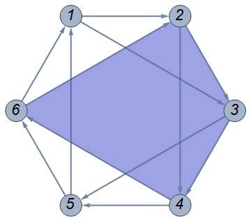
Refer to caption
Refer to caption
Figure 11: Nf=2subscript𝑁𝑓2N_{f}=2 kite-subquivers for the discrete flow T2subscript𝑇2T_{2}

Because we are "popping out" the nodes 1,5 from the quiver, we want to achieve this by implementing the limit (196) directly on the cluster variables. By studying the expressions for the Casimirs (86), (87) we find

x3x6=Q1Q2q1/2,subscript𝑥3subscript𝑥6subscript𝑄1subscript𝑄2superscript𝑞12\displaystyle x_{3}x_{6}=Q_{1}Q_{2}q^{1/2}, x1x4=(Q1Q2t)1,subscript𝑥1subscript𝑥4superscriptsubscript𝑄1subscript𝑄2𝑡1\displaystyle x_{1}x_{4}=(Q_{1}Q_{2}t)^{-1}\rightarrow\infty, x2x5=q1/2t0,subscript𝑥2subscript𝑥5superscript𝑞12𝑡0\displaystyle x_{2}x_{5}=q^{1/2}t\rightarrow 0, (197)

so that we want to study the limit

x1=(x4Q1Q2t)1,subscript𝑥1superscriptsubscript𝑥4subscript𝑄1subscript𝑄2𝑡1\displaystyle x_{1}=(x_{4}Q_{1}Q_{2}t)^{-1}\rightarrow\infty, x5=q1/2tx210.subscript𝑥5superscript𝑞12𝑡superscriptsubscript𝑥210\displaystyle x_{5}=q^{1/2}tx_{2}^{-1}\rightarrow 0. (198)

Taking the limit on the mutations we obtain

μ2(x)=(x1(1+x2),x21,x31+x21,x41+x21,x5,(1+x2)x6)(,x21,x31+x21,x41+x21,0,(1+x2)x6),subscript𝜇2xsubscript𝑥11subscript𝑥2superscriptsubscript𝑥21subscript𝑥31superscriptsubscript𝑥21subscript𝑥41superscriptsubscript𝑥21subscript𝑥51subscript𝑥2subscript𝑥6superscriptsubscript𝑥21subscript𝑥31superscriptsubscript𝑥21subscript𝑥41superscriptsubscript𝑥2101subscript𝑥2subscript𝑥6\begin{split}\mu_{2}(\textbf{x})&=\left(\begin{array}[]{cccccc}x_{1}(1+x_{2}),&x_{2}^{-1},&\frac{x_{3}}{1+x_{2}^{-1}},&\frac{x_{4}}{1+x_{2}^{-1}},&x_{5},&(1+x_{2})x_{6}\end{array}\right)\\ &\rightarrow\left(\begin{array}[]{cccccc}\infty,&x_{2}^{-1},&\frac{x_{3}}{1+x_{2}^{-1}},&\frac{x_{4}}{1+x_{2}^{-1}},&0,&(1+x_{2})x_{6}\end{array}\right),\end{split} (199)

and similarly for the other mutations μ3,μ4,μ6subscript𝜇3subscript𝜇4subscript𝜇6\mu_{3},\mu_{4},\mu_{6}, that all degenerate to the mutations of the four-dimensional quiver. The discrete flow also has a "good" limit:

{T2(x1)=1+x51(1+x2)x6,T2(x2)=x4(1+x5)(x6(1+x2)(1+x51)1)(1+x21)(1+x31(1+x21)(1+x5)),T2(x3)=1+x6(1+x2)(1+x51)1x2(1+x31(1+x21)(1+x5)1),T2(x4)=1+x21x3(1+x5),T2(x5)=x1(1+x2)(1+x3(1+x5)(1+x21)1)(1+x51)(1+x61(1+x51)(1+x2)1),T2(x6)=1+x3(1+x5)(1+x21)1x5(1+x61(1+x51)(1+x2)1)casessubscript𝑇2subscript𝑥11superscriptsubscript𝑥511subscript𝑥2subscript𝑥6otherwisesubscript𝑇2subscript𝑥2subscript𝑥41subscript𝑥5subscript𝑥61subscript𝑥2superscript1superscriptsubscript𝑥5111superscriptsubscript𝑥211superscriptsubscript𝑥311superscriptsubscript𝑥211subscript𝑥5otherwisesubscript𝑇2subscript𝑥31subscript𝑥61subscript𝑥2superscript1superscriptsubscript𝑥511subscript𝑥21superscriptsubscript𝑥311superscriptsubscript𝑥21superscript1subscript𝑥51otherwisesubscript𝑇2subscript𝑥41superscriptsubscript𝑥21subscript𝑥31subscript𝑥5otherwisesubscript𝑇2subscript𝑥5subscript𝑥11subscript𝑥21subscript𝑥31subscript𝑥5superscript1superscriptsubscript𝑥2111superscriptsubscript𝑥511superscriptsubscript𝑥611superscriptsubscript𝑥51superscript1subscript𝑥21otherwisesubscript𝑇2subscript𝑥61subscript𝑥31subscript𝑥5superscript1superscriptsubscript𝑥211subscript𝑥51superscriptsubscript𝑥611superscriptsubscript𝑥51superscript1subscript𝑥21otherwise\displaystyle\begin{cases}T_{2}(x_{1})=\frac{1+x_{5}^{-1}}{(1+x_{2})x_{6}},\\ T_{2}(x_{2})=\frac{x_{4}(1+x_{5})\left(x_{6}(1+x_{2})(1+x_{5}^{-1})^{-1}\right)}{(1+x_{2}^{-1})(1+x_{3}^{-1}(1+x_{2}^{-1})(1+x_{5}))},\\ T_{2}(x_{3})=\frac{1+x_{6}(1+x_{2})(1+x_{5}^{-1})^{-1}}{x_{2}\left(1+x_{3}^{-1}(1+x_{2}^{-1})(1+x_{5})^{-1}\right)},\\ T_{2}(x_{4})=\frac{1+x_{2}^{-1}}{x_{3}(1+x_{5})},\\ T_{2}(x_{5})=\frac{x_{1}(1+x_{2})\left(1+x_{3}(1+x_{5})(1+x_{2}^{-1})^{-1}\right)}{(1+x_{5}^{-1})\left(1+x_{6}^{-1}(1+x_{5}^{-1})(1+x_{2})^{-1}\right)},\\ T_{2}(x_{6})=\frac{1+x_{3}(1+x_{5})(1+x_{2}^{-1})^{-1}}{x_{5}\left(1+x_{6}^{-1}(1+x_{5}^{-1})(1+x_{2})^{-1}\right)}\end{cases} \displaystyle\rightarrow {,x4(1+x21)(1+x31(1+x21)),x31+x2(1+x3),1+x21x3,0,x6(1+x2(1+x3)).casesotherwisesubscript𝑥41superscriptsubscript𝑥211superscriptsubscript𝑥311superscriptsubscript𝑥21otherwisesubscript𝑥31subscript𝑥21subscript𝑥3otherwise1superscriptsubscript𝑥21subscript𝑥3otherwise0otherwisesubscript𝑥61subscript𝑥21subscript𝑥3otherwise\displaystyle\begin{cases}\infty,\\ \frac{x_{4}}{(1+x_{2}^{-1})\left(1+x_{3}^{-1}(1+x_{2}^{-1})\right)},\\ \frac{x_{3}}{1+x_{2}(1+x_{3})},\\ \frac{1+x_{2}^{-1}}{x_{3}},\\ 0,\\ x_{6}\left(1+x_{2}(1+x_{3})\right).\end{cases} (200)

If we call the variables after taking the limit

x4X1,subscript𝑥4subscript𝑋1\displaystyle x_{4}\rightarrow X_{1}, x2X2,subscript𝑥2subscript𝑋2\displaystyle x_{2}\rightarrow X_{2}, x3X3,subscript𝑥3subscript𝑋3\displaystyle x_{3}\rightarrow X_{3}, x6X4,subscript𝑥6subscript𝑋4\displaystyle x_{6}\rightarrow X_{4}, (201)

we have that the limit of the discrete flow is

T2(4d)=(3,2,1)μ3μ2,superscriptsubscript𝑇24𝑑321subscript𝜇3subscript𝜇2T_{2}^{(4d)}=(3,2,1)\mu_{3}\mu_{2}, (202)

which is an automorphism of the 4d quiver. We can follow the same logic for the other discrete flows T1,T3,T4subscript𝑇1subscript𝑇3subscript𝑇4T_{1},T_{3},T_{4}: we will from now on discuss only the limits on the discrete time flows, because those on the mutations are rather simple and given by essentially the same computations as above. In the first case the flow is

T1(Q+)=q1Q+,subscript𝑇1subscript𝑄superscript𝑞1subscript𝑄\displaystyle T_{1}(Q_{+})=q^{-1}Q_{+}, Q+=Q1Q2subscript𝑄subscript𝑄1subscript𝑄2\displaystyle Q_{+}=Q_{1}Q_{2} (203)

so that the natural guess for the right limit to consider is Q+subscript𝑄Q_{+}\rightarrow\infty, in analogy with the previous case. By looking at the Casimirs, we arrive to the conclusion that we can either decouple the nodes 1,3 or 4,6, producing the 4d Nf=2subscript𝑁𝑓2N_{f}=2 subquivers in Figure 12.

Refer to caption
Refer to caption
Figure 12: Nf=2subscript𝑁𝑓2N_{f}=2 kite-subquivers for the discrete flow T1subscript𝑇1T_{1}

The limit we want to implement is then

x4=(x1Q+t)10,subscript𝑥4superscriptsubscript𝑥1subscript𝑄𝑡10\displaystyle x_{4}=(x_{1}Q_{+}t)^{-1}\rightarrow 0, x6=Q+q1/2x31,subscript𝑥6subscript𝑄superscript𝑞12superscriptsubscript𝑥31\displaystyle x_{6}=Q_{+}q^{1/2}x_{3}^{-1}\rightarrow\infty, (204)

which gives

{T1(x1)=x3(1+x4)(1+x5(1+x1)(1+x41)1)x1(1+x21(1+x11)(1+x4)1),T1(x2)=1+x5(1+x1)(1+x41)1x1(1+x21(1+x11)(1+x4)1),T1(x3)=1+x11x2(1+x4),T1(x4)=x6(1+x1)(1+x2(1+x4)(1+x11)1)(1+x41)(1+x51(1+x41)(1+x1)1),T1(x5)=1+x2(1+x4)(1+x11)1x4(1+x51(1+x41)(1+x1)1),T1(x6)=1+x41x5(1+x1).casessubscript𝑇1subscript𝑥1subscript𝑥31subscript𝑥41subscript𝑥51subscript𝑥1superscript1superscriptsubscript𝑥411subscript𝑥11superscriptsubscript𝑥211superscriptsubscript𝑥11superscript1subscript𝑥41otherwisesubscript𝑇1subscript𝑥21subscript𝑥51subscript𝑥1superscript1superscriptsubscript𝑥411subscript𝑥11superscriptsubscript𝑥211superscriptsubscript𝑥11superscript1subscript𝑥41otherwisesubscript𝑇1subscript𝑥31superscriptsubscript𝑥11subscript𝑥21subscript𝑥4otherwisesubscript𝑇1subscript𝑥4subscript𝑥61subscript𝑥11subscript𝑥21subscript𝑥4superscript1superscriptsubscript𝑥1111superscriptsubscript𝑥411superscriptsubscript𝑥511superscriptsubscript𝑥41superscript1subscript𝑥11otherwisesubscript𝑇1subscript𝑥51subscript𝑥21subscript𝑥4superscript1superscriptsubscript𝑥111subscript𝑥41superscriptsubscript𝑥511superscriptsubscript𝑥41superscript1subscript𝑥11otherwisesubscript𝑇1subscript𝑥61superscriptsubscript𝑥41subscript𝑥51subscript𝑥1otherwise\displaystyle\begin{cases}T_{1}(x_{1})=\frac{x_{3}(1+x_{4})\left(1+x_{5}(1+x_{1})(1+x_{4}^{-1})^{-1}\right)}{x_{1}\left(1+x_{2}^{-1}(1+x_{1}^{-1})(1+x_{4})^{-1}\right)},\\ T_{1}(x_{2})=\frac{1+x_{5}(1+x_{1})(1+x_{4}^{-1})^{-1}}{x_{1}\left(1+x_{2}^{-1}(1+x_{1}^{-1})(1+x_{4})^{-1}\right)},\\ T_{1}(x_{3})=\frac{1+x_{1}^{-1}}{x_{2}(1+x_{4})},\\ T_{1}(x_{4})=\frac{x_{6}(1+x_{1})\left(1+x_{2}(1+x_{4})(1+x_{1}^{-1})^{-1}\right)}{(1+x_{4}^{-1})\left(1+x_{5}^{-1}(1+x_{4}^{-1})(1+x_{1})^{-1}\right)},\\ T_{1}(x_{5})=\frac{1+x_{2}(1+x_{4})(1+x_{1}^{-1})^{-1}}{x_{4}\left(1+x_{5}^{-1}(1+x_{4}^{-1})(1+x_{1})^{-1}\right)},\\ T_{1}(x_{6})=\frac{1+x_{4}^{-1}}{x_{5}(1+x_{1})}.\end{cases} \displaystyle\rightarrow {x3(1+x11)(1+x21(1+x11)),x21+x1(1+x2),1+x11x2,0,x5(1+x1(1+x2)),.casessubscript𝑥31superscriptsubscript𝑥111superscriptsubscript𝑥211superscriptsubscript𝑥11otherwisesubscript𝑥21subscript𝑥11subscript𝑥2otherwise1superscriptsubscript𝑥11subscript𝑥2otherwise0otherwisesubscript𝑥51subscript𝑥11subscript𝑥2otherwiseotherwise\displaystyle\begin{cases}\frac{x_{3}}{(1+x_{1}^{-1})(1+x_{2}^{-1}(1+x_{1}^{-1}))},\\ \frac{x_{2}}{1+x_{1}(1+x_{2})},\\ \frac{1+x_{1}^{-1}}{x_{2}},\\ 0,\\ x_{5}\left(1+x_{1}(1+x_{2})\right),\\ \infty.\end{cases} (205)

Which is the same 4d quiver automorphism as for T2subscript𝑇2T_{2}, up to permutations of the nodes. The time evolution T3subscript𝑇3T_{3} is characterized by

T3(Q+)=qQ+,subscript𝑇3subscript𝑄𝑞subscript𝑄\displaystyle T_{3}(Q_{+})=qQ_{+}, T3(t)=q1t,subscript𝑇3𝑡superscript𝑞1𝑡\displaystyle T_{3}(t)=q^{-1}t, (206)

so that the natural limit on the Casimirs is

x3x6=Q+q1/20,subscript𝑥3subscript𝑥6subscript𝑄superscript𝑞120\displaystyle x_{3}x_{6}=Q_{+}q^{1/2}\rightarrow 0, x2x5=q1/2t.subscript𝑥2subscript𝑥5superscript𝑞12𝑡\displaystyle x_{2}x_{5}=q^{1/2}t\rightarrow\infty. (207)

This can be achieved by decoupling the nodes 3,5 or 2,6, keeping the subquivers depicted in Figure 13.
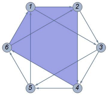
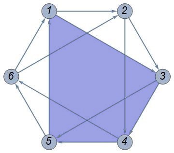
Refer to caption
Refer to caption
Figure 13: Nf=2subscript𝑁𝑓2N_{f}=2 kite-subquivers for the discrete flow T3subscript𝑇3T_{3}

Choosing the former one for concreteness, we want to compute the limit

x3=Q+q1/2x610,subscript𝑥3subscript𝑄superscript𝑞12superscriptsubscript𝑥610\displaystyle x_{3}=Q_{+}q^{1/2}x_{6}^{-1}\rightarrow 0, x5=q1/2tx21,subscript𝑥5superscript𝑞12𝑡superscriptsubscript𝑥21\displaystyle x_{5}=q^{1/2}tx_{2}^{-1}\rightarrow\infty, (208)

on the discrete evolution T3subscript𝑇3T_{3}. This is given by

{T3(x1)=1+x4(1+x6)(1+x31)1x6(1+x11(1+x61)(1+x3)),T3(x2)=1+x61x1(1+x3),T3(x3)=x5(1+x6)(1+x1(1+x3)(1+x61)1)(1+x31)(1+x4(1+x31)(1+x6)1),T3(x4)=1+x1(1+x3)(1+x61)1x3(1+x41(1+x31)(1+x6)1),T3(x5)=1+x31x4(1+x6),T3(x6)=x2(1+x3)(1+x4(1+x6)(1+x31)1)(1+x61)(1+x11(1+x61)(1+x3)1),casessubscript𝑇3subscript𝑥11subscript𝑥41subscript𝑥6superscript1superscriptsubscript𝑥311subscript𝑥61superscriptsubscript𝑥111superscriptsubscript𝑥611subscript𝑥3otherwisesubscript𝑇3subscript𝑥21superscriptsubscript𝑥61subscript𝑥11subscript𝑥3otherwisesubscript𝑇3subscript𝑥3subscript𝑥51subscript𝑥61subscript𝑥11subscript𝑥3superscript1superscriptsubscript𝑥6111superscriptsubscript𝑥311subscript𝑥41superscriptsubscript𝑥31superscript1subscript𝑥61otherwisesubscript𝑇3subscript𝑥41subscript𝑥11subscript𝑥3superscript1superscriptsubscript𝑥611subscript𝑥31superscriptsubscript𝑥411superscriptsubscript𝑥31superscript1subscript𝑥61otherwisesubscript𝑇3subscript𝑥51superscriptsubscript𝑥31subscript𝑥41subscript𝑥6otherwisesubscript𝑇3subscript𝑥6subscript𝑥21subscript𝑥31subscript𝑥41subscript𝑥6superscript1superscriptsubscript𝑥3111superscriptsubscript𝑥611superscriptsubscript𝑥111superscriptsubscript𝑥61superscript1subscript𝑥31otherwise\displaystyle\begin{cases}T_{3}(x_{1})=\frac{1+x_{4}(1+x_{6})(1+x_{3}^{-1})^{-1}}{x_{6}\left(1+x_{1}^{-1}(1+x_{6}^{-1})(1+x_{3})\right)},\\ T_{3}(x_{2})=\frac{1+x_{6}^{-1}}{x_{1}(1+x_{3})},\\ T_{3}(x_{3})=\frac{x_{5}(1+x_{6})\left(1+x_{1}(1+x_{3})(1+x_{6}^{-1})^{-1}\right)}{(1+x_{3}^{-1})\left(1+x_{4}(1+x_{3}^{-1})(1+x_{6})^{-1}\right)},\\ T_{3}(x_{4})=\frac{1+x_{1}(1+x_{3})(1+x_{6}^{-1})^{-1}}{x_{3}\left(1+x_{4}^{-1}(1+x_{3}^{-1})(1+x_{6})^{-1}\right)},\\ T_{3}(x_{5})=\frac{1+x_{3}^{-1}}{x_{4}(1+x_{6})},\\ T_{3}(x_{6})=\frac{x_{2}(1+x_{3})\left(1+x_{4}(1+x_{6})(1+x_{3}^{-1})^{-1}\right)}{(1+x_{6}^{-1})\left(1+x_{1}^{-1}(1+x_{6}^{-1})(1+x_{3})^{-1}\right)},\end{cases} \displaystyle\rightarrow {x11+x6(1+x1),1+x61x1,0,x4(1+x6(1+x1)),,x2(1+x61)(1+x11(1+x61)).casessubscript𝑥11subscript𝑥61subscript𝑥1otherwise1superscriptsubscript𝑥61subscript𝑥1otherwise0otherwisesubscript𝑥41subscript𝑥61subscript𝑥1otherwiseotherwisesubscript𝑥21superscriptsubscript𝑥611superscriptsubscript𝑥111superscriptsubscript𝑥61otherwise\displaystyle\begin{cases}\frac{x_{1}}{1+x_{6}(1+x_{1})},\\ \frac{1+x_{6}^{-1}}{x_{1}},\\ 0,\\ x_{4}(1+x_{6}(1+x_{1})),\\ \infty,\\ \frac{x_{2}}{(1+x_{6}^{-1})(1+x_{1}^{-1}(1+x_{6}^{-1}))}.\end{cases} (209)

We see that in all the cases that yielded the time evolution of q-Painlevé III1subscriptIII1\text{III}_{1}, the degeneration of the time flow produces the same automorphism of an appropriate subquiver. It remains to study the flow T4subscript𝑇4T_{4}, which yielded a q-Painlevé IV time evolution, characterized by

T4(Q)=qQ,subscript𝑇4subscript𝑄𝑞subscript𝑄\displaystyle T_{4}(Q_{-})=qQ_{-}, Q=Q2Q1.subscript𝑄subscript𝑄2subscript𝑄1\displaystyle Q_{-}=\frac{Q_{2}}{Q_{1}}. (210)

In terms of the Casimirs b0,b1subscript𝑏0subscript𝑏1b_{0},b_{1}, this leads to

x2x4x6=(qQ)1/20,subscript𝑥2subscript𝑥4subscript𝑥6superscript𝑞subscript𝑄120\displaystyle x_{2}x_{4}x_{6}=\left(qQ_{-}\right)^{1/2}\rightarrow 0, x1x3x5=q1Q1/2.subscript𝑥1subscript𝑥3subscript𝑥5superscript𝑞1superscriptsubscript𝑄12\displaystyle x_{1}x_{3}x_{5}=q^{-1}Q_{-}^{-1/2}\rightarrow\infty. (211)

To achieve this without affecting the Casimirs a0,a1,a2subscript𝑎0subscript𝑎1subscript𝑎2a_{0},a_{1},a_{2} we have to decouple either the nodes 2,5, or the nodes 3,6, or the nodes 1,4, giving the subquivers in Figure 14, and we will consider the first option, given by the limit

x2=(qQ)1/2x41x610,subscript𝑥2superscript𝑞subscript𝑄12superscriptsubscript𝑥41superscriptsubscript𝑥610\displaystyle x_{2}=(qQ_{-})^{1/2}x_{4}^{-1}x_{6}^{-1}\rightarrow 0, x5=q1Q1/2x11x31.subscript𝑥5superscript𝑞1superscriptsubscript𝑄12superscriptsubscript𝑥11superscriptsubscript𝑥31\displaystyle x_{5}=q^{-1}Q_{-}^{-1/2}x_{1}^{-1}x_{3}^{-1}\rightarrow\infty. (212)
Refer to caption
Refer to caption
Refer to caption
Figure 14: Nf=2subscript𝑁𝑓2N_{f}=2 subquivers for the discrete flow T4subscript𝑇4T_{4}

Here something similar to what happened when we studied the degeneration of the q-Painlevé III3subscriptIII3\text{III}_{3} associated to local 𝔽1subscript𝔽1\mathbb{F}_{1} happens: recall that in that case T𝔽1subscript𝑇subscript𝔽1T_{\mathbb{F}_{1}} did not have a good degeneration limit as an automorphism of the subquiver, but rather its square did. We observed that this was related to the 2subscript2\mathbb{Z}_{2}-periodicity of the action of T𝔽1subscript𝑇subscript𝔽1T_{\mathbb{F}_{1}} on the BPS charges. What happens here is that not T4subscript𝑇4T_{4}, but rather T43superscriptsubscript𝑇43T_{4}^{3} has a good action after taking the limit, in particular only for T43superscriptsubscript𝑇43T_{4}^{3} it is true that

T43(x2)0,superscriptsubscript𝑇43subscript𝑥20\displaystyle T_{4}^{3}(x_{2})\rightarrow 0, T43(x5),superscriptsubscript𝑇43subscript𝑥5\displaystyle T_{4}^{3}(x_{5})\rightarrow\infty, (213)

consistently with the limit.

The resulting sub quiver is the oriented square with arrows of valency one and no diagonals with adjacency matrix

B=(0101101001011010).𝐵0101101001011010B=\left(\begin{array}[]{cccc}0&1&0&-1\\ -1&0&1&0\\ 0&-1&0&1\\ 1&0&-1&0\end{array}\right). (214)

The corresponding four dimensional gauge theory has been already classified in Cecotti:2014zga as Q(1,1)𝑄11Q(1,1) and shown to correspond to H3subscript𝐻3H_{3}, which is the Argyres-Douglas limit of the Nf=3subscript𝑁𝑓3N_{f}=3 with SU(2)𝑆𝑈2SU(2). All this is consistent with the reductions of the Sakai’s table in Figure 1.

The symmetry type of the five dimensional SU(2)𝑆𝑈2SU(2) Nf=2subscript𝑁𝑓2N_{f}=2 gauge theory is E3(1)superscriptsubscript𝐸31E_{3}^{(1)}. The reduction of the T1subscript𝑇1T_{1}, T2subscript𝑇2T_{2} and T3subscript𝑇3T_{3} flows corresponds to the reduction E3(1)D2(1)superscriptsubscript𝐸31superscriptsubscript𝐷21E_{3}^{(1)}\to D_{2}^{(1)}, the latter being the symmetry type of the four dimensional SU(2)𝑆𝑈2SU(2) Nf=2subscript𝑁𝑓2N_{f}=2 gauge theory. The reduction of the T4subscript𝑇4T_{4} flow corresponds to the reduction E3(1)A2(1)superscriptsubscript𝐸31superscriptsubscript𝐴21E_{3}^{(1)}\to A_{2}^{(1)}, the latter being the symmetry type of the H3subscript𝐻3H_{3} theory. According to Sakai’s classification (see Figure 1) and the analysis in Bonelli:2016qwg this flow correctly points to the Argyres-Douglas theory of Nf=3subscript𝑁𝑓3N_{f}=3 which is, in the four dimensional limit, governed by the differential PIV equation.

6 Conclusions and Outlook

In this paper we studied the discrete flows induced by automorphisms of BPS quivers associated to Calabi-Yau geometries engineering five-dimensional quantum field theories. We showed that these flows provide a simple and effective way to determine the BPS spectrum of these theories, producing at the same time a set of bilinear q-difference equations satisfied by the grand canonical partition function of topological string amplitudes. In the rank one case these are known as q-Painlevé equations and admit in a suitable region of the moduli space solutions in terms of Nekrasov-Okounkov, or free fermions, partition functions.

A very attractive feature of this approach is that a simple symmetry principle – the symmetry of the BPS quiver – provides strong constraints on the BPS spectrum and contains a rich and deep set of information which goes well beyond the perturbative approaches to the same theories. Indeed, one can show that the non-perturbative completion of topological string via a spectral determinant presentation, arising in the context of the topological string/ spectral theory correspondence, arises naturally as solution of this system of discrete flow equations Bonelli:2017gdk . Moreover, some of the flows associated to the BPS quiver directly link to non-perturbative phases of the corresponding gauge theory, as we have seen for a particular flow of the local dP3𝑑subscript𝑃3dP_{3} geometry which describe a (A1,D4)subscript𝐴1subscript𝐷4(A_{1},D_{4}) Argyres-Douglas point, see subsect. 5.3. A discussion of the relation between Painlevé equations and Argyres-Douglas points of four-dimensional gauge theories can be found in Bonelli:2016qwg based on the class 𝒮𝒮{\cal S} description of these theories Bonelli:2011aa .

It is also very interesting that a fully classical construction, the cluster algebra associated to the BPS quiver, contains information about the quantum geometry of the Calabi-Yau. Indeed the zeroes of the τ𝜏\tau-functions of the cluster algebra provide the exact spectrum of the associated quantum integrable system, as it was shown in Bonelli:2017gdk for the local 𝔽0subscript𝔽0\mathbb{F}_{0} geometry corresponding to relativistic Toda chain Hatsuda:2015qzx , and in Bonelli:2016idi ; Sciarappa:2017hds for its four-dimensional/non-relativistic limit. Further evidence we provide in this paper is that the X-cluster variables of the 5d quiver flow in the 4d limit to the X-cluster variables of the corresponding four-dimensional BPS quiver, which are known to be related to the Voros symbols, i.e. exponential of the exact quantum WKB periods of the four-dimensional integrable system Iwaki_2014 . The fact the we find that standard topological string – or equivalently 5d gauge theory in the self-dual ΩΩ\Omega-background ϵ1+ϵ2=0subscriptitalic-ϵ1subscriptitalic-ϵ20\epsilon_{1}+\epsilon_{2}=0 rather than in the Nekrasov-Shatashvili Nekrasov:2009rc background ϵ1=0subscriptitalic-ϵ10\epsilon_{1}=0 – provides a quantisation of the Calabi-Yau geometry is not fully surprising from the view point of equivariant localisation. Indeed the difference between the two cases resides in a different choice of one-parameter subgroup of the full toric action, and therefore contains the same amount of information, although under possibly very non-trivial combinatorial identities. A first instance of this phenomenon was discussed from the mathematical perspective in Nakajima:2003uh . For the case at hand, the non-trivial relation between the two approaches is encoded in a suitable limit of blow-up equations Grassi:2018spf ; Grassi:2019coc ; Gavrylenko:2020gjb ; Nekrasov:2020qcq ; Jeong:2020uxz .

There are several directions to further investigate.

Let us notice that, with respect to the framework of Alim:2011ae ; Alim:2011kw , to define a BPS chamber one should set the precise order of the arguments of the central charges Z(γi)𝑍subscript𝛾𝑖Z(\gamma_{i}) for all the charges γisubscript𝛾𝑖\gamma_{i} in the spectrum. While our method efficiently computes the spectrum, at least in the tame chambers, it doesn’t point yet to a precise definition of the corresponding moduli values. This is because we still miss a link with the relevant stability conditions. Our method relies on the existence of patches in the moduli space where the topological string partition function allows finite radius converging expansions888See also the comments at the end of the subsection 4.2 on this point.. Let us notice that clarifying this point would prepare the skeleton of the demonstration that Kontsevich-Soibelman wall-crossing would be equivalent to the discrete equations (q-Painlevé and higher rank analogues) we obtain. Moreover, the chambers we do compute are "triangular" in the sense of Cecotti:2015qha . In this paper it is shown that similar chambers exist for all the class 𝒮[A1]𝒮delimited-[]subscript𝐴1{\cal S}[A_{1}] theories: while multiple affinizations are generically involved, these coincide with the ones computed with our methods, at least in the examples we work out explicitly.

We have seen that when the Calabi-Yau geometry admits several moduli there are various inequivalent flows for the same BPS quiver, but only few of them have a realisation in terms of weakly coupled Lagrangian field theories. In some cases the other flows correspond simply to Bäcklund transformations mapping solutions one into the others. This is the case for example for the fluxes T1,T2,T3subscript𝑇1subscript𝑇2subscript𝑇3T_{1},T_{2},T_{3} discussed in subsect. 3.3. We expect that the full solution to this system of equations will be given in terms of suitable expansions of the topological vertex999Similar considerations appeared in Coman:2018uwk ; Coman:2020qgf for the four dimensional case. Aganagic:2003db , while its non-pertubative completion should be given by the spectral determinant of the corresponding Nf=2subscript𝑁𝑓2N_{f}=2 spectral curve. In other cases the flows are intrinsically non-perturbative, like the flux T4subscript𝑇4T_{4} discussed in subsect.5.3. It would be interesting to characterise the solutions of these flows in terms of supersymmetric indices of four-dimensional gauge theories Cordova:2015nma ; Maruyoshi:2016tqk ; Maruyoshi:2016aim .

We expect that the full refined topological string or equivalently the gauge theory in the full ΩΩ\Omega background is captured by the quantum cluster algebra. The bilinear equations in this case are expected to have a direct relation to the K-theoretic blow-up equations Bershtein:2018zcz .

We have also shown that the X-cluster variables correctly reproduce the ones of the four dimensional BPS quivers under a suitable scaling limit. It would be very interesting to further explore the relation of our results with the ones on exact WKB methods and TBA equations Gaiotto:2009hg ; Grassi:2019coc ; FIORAVANTI2020135376 , possibly extending these methods to the q-difference/5d case. For the class S theories an important rôle should be played by the group Hitchin system Elliott:2018yqm , in the perspective of its quantisation Bonelli:2009zp ; Bonelli:2011na . An interesting open question is the nature of the quantum periods in five dimensions and their relation to the cluster variables appearing in the study of q-Painlevé equations.

In the four-dimensional case, the Painlevé/gauge theory correspondence Bonelli:2016qwg extends also to non-toric cases, corresponding to isomonodromic deformation problems on higher genus Riemann surfaces, see Bonelli:2019boe ; Bonelli:2019yjd for the genus one case. These have a 5d uplift in terms of q-Virasoro algebra Mironov:2017sqp and matrix models Nedelin:2015mio ; Lodin:2018lbz whose BPS quiver interpretation would be more than welcome. Also the higher rank extension of BPS quiver flows and the associated tau-functions is to be explored in detail. As a first example, one can consider SU(N)𝑆𝑈𝑁SU(N) Super Yang-Mills, whose spectral determinant in matrix model presentation was presented in Bonelli:2017ptp . In the one period phase, this satisfies N𝑁N-particle Toda chain equations. The corresponding cluster integrable system is discussed in Bershtein:2018srt . More in general, our method should extend beyond the rank 111 case and q-Painlevé systems, pointing to more general results about topological string partition functions and discrete dynamical systems.

Acknowledgements: We would like to thank M. Cirafici, D. Fioravanti, M. Semenyakin, A. Marshakov for interesting discussions. Many thanks also to M. Del Zotto and P. Gavrylenko for a careful reading of the manuscript and interesting comments.

The research of G.B. and F.DM. is partly supported by the INFN Iniziativa Specifica ST&FI and by the PRIN project “Non-perturbative Aspects Of Gauge Theories And Strings”. The research of A.T. is partly supported by the INFN Iniziativa Specifica GAST and by the PRIN project “Geometria delle varietà algebriche”.

Appendix A q-Special functions and Nekrasov functions

The 5d instanton partition function Nekrasov:2003af ; Bruzzo:2002xf for 𝒩=1𝒩1\mathcal{N}=1 5d SU(N)𝑆𝑈𝑁SU(N) SYM with Nfsubscript𝑁𝑓N_{f} fundamental flavors and Chern-Simons level k=0,1,,N1𝑘01𝑁1k=0,1,\dots,N-1 is given by a sum over N-tuples if partitions 𝝀(λ1,,λN)𝝀subscript𝜆1subscript𝜆𝑁\boldsymbol{\lambda}(\lambda_{1},\dots,\lambda_{N}) with counting parameter t𝑡t:

Zinst=𝝀t|𝝀|Z𝝀CSZ𝝀fundZ𝝀gauge.subscript𝑍𝑖𝑛𝑠𝑡subscript𝝀superscript𝑡𝝀subscriptsuperscript𝑍𝐶𝑆𝝀superscriptsubscript𝑍𝝀𝑓𝑢𝑛𝑑superscriptsubscript𝑍𝝀𝑔𝑎𝑢𝑔𝑒Z_{inst}=\sum_{\boldsymbol{\lambda}}t^{|\boldsymbol{\lambda}|}Z^{CS}_{\boldsymbol{\lambda}}Z_{\boldsymbol{\lambda}}^{fund}Z_{\boldsymbol{\lambda}}^{gauge}. (215)

The Chern-Simons factor given by

Z𝝀CS=i=1NTλi(ui;q1,q2)k,subscriptsuperscript𝑍𝐶𝑆𝝀superscriptsubscriptproduct𝑖1𝑁subscript𝑇subscript𝜆𝑖superscriptsubscript𝑢𝑖subscript𝑞1subscript𝑞2𝑘\displaystyle Z^{CS}_{\boldsymbol{\lambda}}=\prod_{i=1}^{N}T_{\lambda_{i}}(u_{i};q_{1},q_{2})^{k}, Tλ(u;q1,q2)=(i,j)λuq1i1q2j1,subscript𝑇𝜆𝑢subscript𝑞1subscript𝑞2subscriptproduct𝑖𝑗𝜆𝑢superscriptsubscript𝑞1𝑖1superscriptsubscript𝑞2𝑗1\displaystyle T_{\lambda}(u;q_{1},q_{2})=\prod_{(i,j)\in\lambda}uq_{1}^{i-1}q_{2}^{j-1}, (216)

while the matter and gauge contributions can all be written in terms of the single building block

Nλ,μ(u,q1,q2)=sλ(1uq2aμ(s)1q1lλ(s))sμ(1uq2aλ(s)q1lμ(s)1),subscript𝑁𝜆𝜇𝑢subscript𝑞1subscript𝑞2subscriptproduct𝑠𝜆1𝑢superscriptsubscript𝑞2subscript𝑎𝜇𝑠1superscriptsubscript𝑞1subscript𝑙𝜆𝑠subscriptproduct𝑠𝜇1𝑢superscriptsubscript𝑞2subscript𝑎𝜆𝑠superscriptsubscript𝑞1subscript𝑙𝜇𝑠1N_{\lambda,\mu}(u,q_{1},q_{2})=\prod_{s\in\lambda}\left(1-uq_{2}^{-a_{\mu}(s)-1}q_{1}^{l_{\lambda}(s)}\right)\prod_{s\in\mu}\left(1-uq_{2}^{a_{\lambda}(s)}q_{1}^{-l_{\mu}(s)-1}\right), (217)

in the following way:

Z𝝀fund=i=1Nfα=1NNλ,(Qiuα),subscriptsuperscript𝑍𝑓𝑢𝑛𝑑𝝀superscriptsubscriptproduct𝑖1subscript𝑁𝑓superscriptsubscriptproduct𝛼1𝑁subscript𝑁𝜆subscript𝑄𝑖subscript𝑢𝛼Z^{fund}_{\boldsymbol{\lambda}}=\prod_{i=1}^{N_{f}}\prod_{\alpha=1}^{N}N_{\lambda,\emptyset}(Q_{i}u_{\alpha}), (218)
Z𝝀gauge=i,j=1N1Nλi,λj(ui/uj;q1,q2).superscriptsubscript𝑍𝝀𝑔𝑎𝑢𝑔𝑒superscriptsubscriptproduct𝑖𝑗1𝑁1subscript𝑁subscript𝜆𝑖subscript𝜆𝑗subscript𝑢𝑖subscript𝑢𝑗subscript𝑞1subscript𝑞2Z_{\boldsymbol{\lambda}}^{gauge}=\prod_{i,j=1}^{N}\frac{1}{N_{\lambda_{i},\lambda_{j}}(u_{i}/u_{j};q_{1},q_{2})}. (219)

The perturbative contribution is given by the following:

Zcl=elogti=1N(logui)22logq1logq2ki=1N(logui)36logq1logq2,subscript𝑍𝑐𝑙superscript𝑒𝑡superscriptsubscript𝑖1𝑁superscriptsubscript𝑢𝑖22subscript𝑞1subscript𝑞2𝑘superscriptsubscript𝑖1𝑁superscriptsubscript𝑢𝑖36subscript𝑞1subscript𝑞2Z_{cl}=e^{-\log t\frac{\sum_{i=1}^{N}(\log u_{i})^{2}}{2\log q_{1}\log q_{2}}-k\frac{\sum_{i=1}^{N}(\log u_{i})^{3}}{6\log q_{1}\log q_{2}}}, (220)
Z1-loop=1αβN(uα/uβ;q1,q2)i=1Nfα=1N(Qiuα;q1,q2).subscript𝑍1-loopsubscriptproduct1𝛼𝛽𝑁subscriptsubscript𝑢𝛼subscript𝑢𝛽subscript𝑞1subscript𝑞2superscriptsubscriptproduct𝑖1subscript𝑁𝑓superscriptsubscriptproduct𝛼1𝑁subscriptsubscript𝑄𝑖subscript𝑢𝛼subscript𝑞1subscript𝑞2Z_{\text{1-loop}}=\frac{\prod_{1\leq\alpha\neq\beta\leq N}\left(u_{\alpha}/u_{\beta};q_{1},q_{2}\right)_{\infty}}{\prod_{i=1}^{N_{f}}\prod_{\alpha=1}^{N}\left(Q_{i}u_{\alpha};q_{1},q_{2}\right)_{\infty}}. (221)

Here (ui/uj;q1,q2)subscriptsubscript𝑢𝑖subscript𝑢𝑗subscript𝑞1subscript𝑞2\left(u_{i}/u_{j};q_{1},q_{2}\right)_{\infty} is the multiple q-Pochhammer symbol, defined by

(z;q1,,qn)i1,,iN=0(1zk=1nqkik)=exp(m=1zmmk=1N11qkm).subscript𝑧subscript𝑞1subscript𝑞𝑛superscriptsubscriptproductsubscript𝑖1subscript𝑖𝑁01𝑧superscriptsubscriptproduct𝑘1𝑛superscriptsubscript𝑞𝑘subscript𝑖𝑘superscriptsubscript𝑚1superscript𝑧𝑚𝑚superscriptsubscriptproduct𝑘1𝑁11superscriptsubscript𝑞𝑘𝑚(z;q_{1},\dots,q_{n})_{\infty}\equiv\prod_{i_{1},\dots,i_{N}=0}^{\infty}\left(1-z\prod_{k=1}^{n}q_{k}^{i_{k}}\right)=\exp\left(-\sum_{m=1}^{\infty}\frac{z^{m}}{m}\prod_{k=1}^{N}\frac{1}{1-q_{k}^{m}}\right). (222)

In all the formulae above the following notations are used, in terms of the four-dimensional gauge theory parameters:

uα=eβaα,subscript𝑢𝛼superscript𝑒𝛽subscript𝑎𝛼\displaystyle u_{\alpha}=e^{\beta a_{\alpha}}, Qi=eβmi,subscript𝑄𝑖superscript𝑒𝛽subscript𝑚𝑖\displaystyle Q_{i}=e^{-\beta m_{i}}, q1=eβϵ1,subscript𝑞1superscript𝑒𝛽subscriptitalic-ϵ1\displaystyle q_{1}=e^{\beta\epsilon_{1}}, q2=eβϵ2.subscript𝑞2superscript𝑒𝛽subscriptitalic-ϵ2\displaystyle q_{2}=e^{\beta\epsilon_{2}}. (223)

An important property of the double Pochhammer symbol, that has to be used repeatedly when solving the bilinear equations, is the following:

(zq;q,q1)(z;q,q1)=(zq;q),subscript𝑧𝑞𝑞superscript𝑞1subscript𝑧𝑞superscript𝑞1subscript𝑧𝑞𝑞\displaystyle\frac{\left(zq;q,q^{-1}\right)_{\infty}}{\left(z;q,q^{-1}\right)_{\infty}}=\left(zq;q\right)_{\infty}, (zq1;q,q1)(z;q,q1)=1(z;q),subscript𝑧superscript𝑞1𝑞superscript𝑞1subscript𝑧𝑞superscript𝑞11subscript𝑧𝑞\displaystyle\frac{\left(zq^{-1};q,q^{-1}\right)_{\infty}}{\left(z;q,q^{-1}\right)_{\infty}}=\frac{1}{\left(z;q\right)_{\infty}}, (224)
(zq;q,)(z;q)=11z.\frac{\left(zq;q,\right)_{\infty}}{\left(z;q\right)_{\infty}}=\frac{1}{1-z}. (225)

The full partition function Z(u;t)𝑍𝑢𝑡Z(u;t) is given by Z=ZclZ1loopZinst𝑍subscript𝑍𝑐𝑙subscript𝑍1loopsubscript𝑍𝑖𝑛𝑠𝑡Z=Z_{cl}Z_{\rm 1-loop}Z_{inst}.

Appendix B q-Painlevé III and IV in Tsuda’s parametrization

We provide here the choice of parameters for the cluster algebra that reproduces the q-Painlevè III1𝐼𝐼subscript𝐼1III_{1} and IV𝐼𝑉IV equations of 2006LMaPh..75…39T . It turns out for this to be useful to introduce

u1=a1(b1b0)1/3,subscript𝑢1subscript𝑎1superscriptsubscript𝑏1subscript𝑏013\displaystyle u_{1}=a_{1}\left(\frac{b_{1}}{b_{0}}\right)^{1/3}, u2=a2(b0b1)1/3,subscript𝑢2subscript𝑎2superscriptsubscript𝑏0subscript𝑏113\displaystyle u_{2}=a_{2}\left(\frac{b_{0}}{b_{1}}\right)^{1/3}, u3=a0(b1b0)1/3,subscript𝑢3subscript𝑎0superscriptsubscript𝑏1subscript𝑏013\displaystyle u_{3}=a_{0}\left(\frac{b_{1}}{b_{0}}\right)^{1/3}, (226)
u4=a1(b0b1)1/3,subscript𝑢4subscript𝑎1superscriptsubscript𝑏0subscript𝑏113\displaystyle u_{4}=a_{1}\left(\frac{b_{0}}{b_{1}}\right)^{1/3}, u5=a2(b1b0)1/3,subscript𝑢5subscript𝑎2superscriptsubscript𝑏1subscript𝑏013\displaystyle u_{5}=a_{2}\left(\frac{b_{1}}{b_{0}}\right)^{1/3}, u6=a0(b0b1)1/3,subscript𝑢6subscript𝑎0superscriptsubscript𝑏0subscript𝑏113\displaystyle u_{6}=a_{0}\left(\frac{b_{0}}{b_{1}}\right)^{1/3}, (227)

Note that in 2006LMaPh..75…39T the Casimirs have a geometric meaning in terms of points blown-up on 1×1superscript1superscript1\mathbb{P}^{1}\times\mathbb{P}^{1}.

B.1 qPIII

Let us consider first the cas of qPIII. We choose as basis for the tropical semifield four independent Casimirs, and parametrize in terms of them the yisubscript𝑦𝑖y_{i}’s in such a way that (86) and (87) are satisfied, together with the correct time evolution (91). We choose as independent Casimirs a1,a2,q,b0subscript𝑎1subscript𝑎2𝑞subscript𝑏0a_{1},a_{2},q,b_{0}. To match with 2006LMaPh..75…39T , we also have to make a different choice for the time evolution parameter q𝑞q,

q=iyi1/2.𝑞subscriptproduct𝑖superscriptsubscript𝑦𝑖12q=\prod_{i}y_{i}^{-1/2}. (228)

Set

y1=q1/3b02/3a11,subscript𝑦1superscript𝑞13superscriptsubscript𝑏023superscriptsubscript𝑎11\displaystyle y_{1}=q^{-1/3}b_{0}^{2/3}a_{1}^{-1}, y2=q1/3b02/3a21,subscript𝑦2superscript𝑞13superscriptsubscript𝑏023superscriptsubscript𝑎21\displaystyle y_{2}=q^{1/3}b_{0}^{2/3}a_{2}^{-1}, y3=q4/3b02/3a1a2,subscript𝑦3superscript𝑞43superscriptsubscript𝑏023subscript𝑎1subscript𝑎2\displaystyle y_{3}=q^{-4/3}b_{0}^{2/3}a_{1}a_{2}, (229)
y4=q1/3b02/3a11,subscript𝑦4superscript𝑞13superscriptsubscript𝑏023superscriptsubscript𝑎11\displaystyle y_{4}=q^{1/3}b_{0}^{-2/3}a_{1}^{-1}, y5=q1/3b02/3a21,subscript𝑦5superscript𝑞13superscriptsubscript𝑏023superscriptsubscript𝑎21\displaystyle y_{5}=q^{-1/3}b_{0}^{2/3}a_{2}^{-1}, y6=q2/3b02/3a1a2.subscript𝑦6superscript𝑞23superscriptsubscript𝑏023subscript𝑎1subscript𝑎2\displaystyle y_{6}=q^{-2/3}b_{0}^{-2/3}a_{1}a_{2}. (230)

The time evolution is the following (we only write the relevant τ𝜏\tau-variables):

{τ2¯=τ4,τ3¯=a2b02/3τ3τ4+q1/3τ1τ6τ2,τ5¯=τ1,τ6¯=q1/3a2τ1τ6+τ3τ4b02/3τ5,,cases¯subscript𝜏2subscript𝜏4otherwise¯subscript𝜏3subscript𝑎2superscriptsubscript𝑏023subscript𝜏3subscript𝜏4superscript𝑞13subscript𝜏1subscript𝜏6subscript𝜏2otherwise¯subscript𝜏5subscript𝜏1otherwise¯subscript𝜏6superscript𝑞13subscript𝑎2subscript𝜏1subscript𝜏6subscript𝜏3subscript𝜏4superscriptsubscript𝑏023subscript𝜏5otherwise\displaystyle\begin{cases}\overline{\tau_{2}}=\tau_{4},\\ \overline{\tau_{3}}=\frac{a_{2}b_{0}^{2/3}\tau_{3}\tau_{4}+q^{1/3}\tau_{1}\tau_{6}}{\tau_{2}},\\ \overline{\tau_{5}}=\tau_{1},\\ \overline{\tau_{6}}=\frac{q^{1/3}a_{2}\tau_{1}\tau_{6}+\tau_{3}\tau_{4}b_{0}^{2/3}}{\tau_{5}},\end{cases}, {τ1¯=τ5,τ3¯=a1b02/3τ5τ6+q1/3τ2τ3τ4,τ4¯=τ2,τ6¯=q1/3a1τ2τ3+b02/3τ5τ6,cases¯subscript𝜏1subscript𝜏5otherwise¯subscript𝜏3subscript𝑎1superscriptsubscript𝑏023subscript𝜏5subscript𝜏6superscript𝑞13subscript𝜏2subscript𝜏3subscript𝜏4otherwise¯subscript𝜏4subscript𝜏2otherwise¯subscript𝜏6superscript𝑞13subscript𝑎1subscript𝜏2subscript𝜏3superscriptsubscript𝑏023subscript𝜏5subscript𝜏6,otherwise\displaystyle\begin{cases}\underline{\tau_{1}}=\tau_{5},\\ \underline{\tau_{3}}=\frac{a_{1}b_{0}^{2/3}\tau_{5}\tau_{6}+q^{1/3}\tau_{2}\tau_{3}}{\tau_{4}},\\ \underline{\tau_{4}}=\tau_{2},\\ \underline{\tau_{6}}=\frac{q^{1/3}a_{1}\tau_{2}\tau_{3}+b_{0}^{2/3}\tau_{5}\tau_{6}}{,}\end{cases} (231)

leading to the bilinear equations

τ3¯τ2=q1/3(τ5¯τ6+u2τ3τ2¯),¯subscript𝜏3subscript𝜏2superscript𝑞13¯subscript𝜏5subscript𝜏6subscript𝑢2subscript𝜏3¯subscript𝜏2\displaystyle\overline{\tau_{3}}\tau_{2}=q^{1/3}(\overline{\tau_{5}}\tau_{6}+u_{2}\tau_{3}\overline{\tau_{2}}), τ6¯τ5=b02/3(u5τ5¯τ6+τ3τ2¯),¯subscript𝜏6subscript𝜏5superscriptsubscript𝑏023subscript𝑢5¯subscript𝜏5subscript𝜏6subscript𝜏3¯subscript𝜏2\displaystyle\overline{\tau_{6}}\tau_{5}=b_{0}^{2/3}(u_{5}\overline{\tau_{5}}\tau_{6}+\tau_{3}\overline{\tau_{2}}), (232)
τ2¯τ3¯=q1/3(u4τ5τ6+τ2τ3),¯subscript𝜏2¯subscript𝜏3superscript𝑞13subscript𝑢4subscript𝜏5subscript𝜏6subscript𝜏2subscript𝜏3\displaystyle\overline{\tau_{2}}\underline{\tau_{3}}=q^{1/3}(u_{4}\tau_{5}\tau_{6}+\tau_{2}\tau_{3}), τ5¯τ6¯=b02/3(u1τ2τ3+τ5τ6).¯subscript𝜏5¯subscript𝜏6superscriptsubscript𝑏023subscript𝑢1subscript𝜏2subscript𝜏3subscript𝜏5subscript𝜏6\displaystyle\overline{\tau_{5}}\underline{\tau_{6}}=b_{0}^{2/3}(u_{1}\tau_{2}\tau_{3}+\tau_{5}\tau_{6}). (233)

These differ from the bilinear equations of 2006LMaPh..75…39T by different overall factors of the RHS, so in principle it would seem that they are different bilinear equations. However they are still equivalent to qPIII. If we define

f=τ5τ6τ2τ3,𝑓subscript𝜏5subscript𝜏6subscript𝜏2subscript𝜏3\displaystyle f=\frac{\tau_{5}\tau_{6}}{\tau_{2}\tau_{3}}, g=τ1τ6τ3τ4,𝑔subscript𝜏1subscript𝜏6subscript𝜏3subscript𝜏4\displaystyle g=\frac{\tau_{1}\tau_{6}}{\tau_{3}\tau_{4}}, (234)

we get the system of first-order q-difference equations

f¯f=a2gg+u51g+u2,¯𝑓𝑓subscript𝑎2𝑔𝑔superscriptsubscript𝑢51𝑔subscript𝑢2\displaystyle\overline{f}f=a_{2}g\frac{g+u_{5}^{-1}}{g+u_{2}}, g¯g=fa1f+u1f+u41,¯𝑔𝑔𝑓subscript𝑎1𝑓subscript𝑢1𝑓superscriptsubscript𝑢41\displaystyle\overline{g}g=\frac{f}{a_{1}}\frac{f+u_{1}}{f+u_{4}^{-1}}, (235)

which is the qPIII equation appearing in 2006LMaPh..75…39T .

B.2 qPIV

The action of T4subscript𝑇4T_{4} on the tau function is the following:

{τ1¯=τ4,τ2¯=q4/3b02/3τ4τ5τ6+a1q5/3τ2τ3τ4+a1a2b04/3τ1τ2τ6τ1τ3,τ3¯=τ6,τ4¯=q5/3τ4τ5τ6+a1b04/3τ2τ3τ4+a1a2q1/3b02/3τ1τ2τ6τ3τ5,τ5¯=τ2,τ6¯=b04/3τ4τ5τ6+q1/3a1b02/3τ2τ3τ4+q2/3a1a2τ1τ2τ6τ1τ5,cases¯subscript𝜏1subscript𝜏4otherwise¯subscript𝜏2superscript𝑞43superscriptsubscript𝑏023subscript𝜏4subscript𝜏5subscript𝜏6subscript𝑎1superscript𝑞53subscript𝜏2subscript𝜏3subscript𝜏4subscript𝑎1subscript𝑎2superscriptsubscript𝑏043subscript𝜏1subscript𝜏2subscript𝜏6subscript𝜏1subscript𝜏3otherwise¯subscript𝜏3subscript𝜏6otherwise¯subscript𝜏4superscript𝑞53subscript𝜏4subscript𝜏5subscript𝜏6subscript𝑎1superscriptsubscript𝑏043subscript𝜏2subscript𝜏3subscript𝜏4subscript𝑎1subscript𝑎2superscript𝑞13superscriptsubscript𝑏023subscript𝜏1subscript𝜏2subscript𝜏6subscript𝜏3subscript𝜏5otherwise¯subscript𝜏5subscript𝜏2otherwise¯subscript𝜏6superscriptsubscript𝑏043subscript𝜏4subscript𝜏5subscript𝜏6superscript𝑞13subscript𝑎1superscriptsubscript𝑏023subscript𝜏2subscript𝜏3subscript𝜏4superscript𝑞23subscript𝑎1subscript𝑎2subscript𝜏1subscript𝜏2subscript𝜏6subscript𝜏1subscript𝜏5otherwise\displaystyle\begin{cases}\overline{\tau_{1}}=\tau_{4},\\ \overline{\tau_{2}}=\frac{q^{4/3}b_{0}^{2/3}\tau_{4}\tau_{5}\tau_{6}+a_{1}q^{5/3}\tau_{2}\tau_{3}\tau_{4}+a_{1}a_{2}b_{0}^{4/3}\tau_{1}\tau_{2}\tau_{6}}{\tau_{1}\tau_{3}},\\ \overline{\tau_{3}}=\tau_{6},\\ \overline{\tau_{4}}=\frac{q^{5/3}\tau_{4}\tau_{5}\tau_{6}+a_{1}b_{0}^{4/3}\tau_{2}\tau_{3}\tau_{4}+a_{1}a_{2}q^{1/3}b_{0}^{2/3}\tau_{1}\tau_{2}\tau_{6}}{\tau_{3}\tau_{5}},\\ \overline{\tau_{5}}=\tau_{2},\\ \overline{\tau_{6}}=\frac{b_{0}^{4/3}\tau_{4}\tau_{5}\tau_{6}+q^{1/3}a_{1}b_{0}^{2/3}\tau_{2}\tau_{3}\tau_{4}+q^{2/3}a_{1}a_{2}\tau_{1}\tau_{2}\tau_{6}}{\tau_{1}\tau_{5}},\end{cases} (236)
{τ1¯=q2/3b04/3τ1τ2τ3+q1/3a1τ1τ5τ6+a1a2b02/3τ3τ4τ5τ2τ6,τ2¯=τ5,τ3¯=q2/3τ1τ2τ3+q1/3a1b02/3τ1τ5τ6+a1a2b04/3τ3τ4τ5τ2τ4,τ4¯=τ1,τ5¯=q2/3b02/3τ1τ2τ3+q1/3a1b04/3τ1τ5τ6+a1a2τ3τ4τ5τ4τ6,τ6¯=τ3.cases¯subscript𝜏1superscript𝑞23superscriptsubscript𝑏043subscript𝜏1subscript𝜏2subscript𝜏3superscript𝑞13subscript𝑎1subscript𝜏1subscript𝜏5subscript𝜏6subscript𝑎1subscript𝑎2superscriptsubscript𝑏023subscript𝜏3subscript𝜏4subscript𝜏5subscript𝜏2subscript𝜏6otherwise¯subscript𝜏2subscript𝜏5otherwise¯subscript𝜏3superscript𝑞23subscript𝜏1subscript𝜏2subscript𝜏3superscript𝑞13subscript𝑎1superscriptsubscript𝑏023subscript𝜏1subscript𝜏5subscript𝜏6subscript𝑎1subscript𝑎2superscriptsubscript𝑏043subscript𝜏3subscript𝜏4subscript𝜏5subscript𝜏2subscript𝜏4otherwise¯subscript𝜏4subscript𝜏1otherwise¯subscript𝜏5superscript𝑞23superscriptsubscript𝑏023subscript𝜏1subscript𝜏2subscript𝜏3superscript𝑞13subscript𝑎1superscriptsubscript𝑏043subscript𝜏1subscript𝜏5subscript𝜏6subscript𝑎1subscript𝑎2subscript𝜏3subscript𝜏4subscript𝜏5subscript𝜏4subscript𝜏6otherwise¯subscript𝜏6subscript𝜏3otherwise\begin{cases}\underline{\tau_{1}}=\frac{q^{2/3}b_{0}^{4/3}\tau_{1}\tau_{2}\tau_{3}+q^{1/3}a_{1}\tau_{1}\tau_{5}\tau_{6}+a_{1}a_{2}b_{0}^{2/3}\tau_{3}\tau_{4}\tau_{5}}{\tau_{2}\tau_{6}},\\ \underline{\tau_{2}}=\tau_{5},\\ \underline{\tau_{3}}=\frac{q^{2/3}\tau_{1}\tau_{2}\tau_{3}+q^{1/3}a_{1}b_{0}^{2/3}\tau_{1}\tau_{5}\tau_{6}+a_{1}a_{2}b_{0}^{4/3}\tau_{3}\tau_{4}\tau_{5}}{\tau_{2}\tau_{4}},\\ \underline{\tau_{4}}=\tau_{1},\\ \underline{\tau_{5}}=\frac{q^{2/3}b_{0}^{2/3}\tau_{1}\tau_{2}\tau_{3}+q^{1/3}a_{1}b_{0}^{4/3}\tau_{1}\tau_{5}\tau_{6}+a_{1}a_{2}\tau_{3}\tau_{4}\tau_{5}}{\tau_{4}\tau_{6}},\\ \underline{\tau_{6}}=\tau_{3}.\end{cases} (237)

At a first glance these seem trilinear, rather than bilinear, equations. However, take linear combinations of (236) in such a way that the first term on the RHS cancels out:

{τ6¯τ1b04/3q5/3τ4¯τ3=τ2τ3τ4a1(q1/3b02/3q5/3b04/3)+a1a2τ1τ2τ6(q2/3b04/3q4/3)τ5,τ6¯τ5b02/3q4/3τ¯2τ3=a1a2τ1τ2τ6(q2/3b02/3q4/3b04/3)τ1,τ4¯τ5q1/3b02/3τ2¯τ1=τ2τ3τ4a1q4/3(q5/3b04/3q1/3b02/3)+a1a2τ1τ2τ6(1b02/3)τ3.cases¯subscript𝜏6subscript𝜏1superscriptsubscript𝑏043superscript𝑞53¯subscript𝜏4subscript𝜏3subscript𝜏2subscript𝜏3subscript𝜏4subscript𝑎1superscript𝑞13superscriptsubscript𝑏023superscript𝑞53superscriptsubscript𝑏043subscript𝑎1subscript𝑎2subscript𝜏1subscript𝜏2subscript𝜏6superscript𝑞23superscriptsubscript𝑏043superscript𝑞43subscript𝜏5otherwise¯subscript𝜏6subscript𝜏5superscriptsubscript𝑏023superscript𝑞43subscript¯𝜏2subscript𝜏3subscript𝑎1subscript𝑎2subscript𝜏1subscript𝜏2subscript𝜏6superscript𝑞23superscriptsubscript𝑏023superscript𝑞43superscriptsubscript𝑏043subscript𝜏1otherwise¯subscript𝜏4subscript𝜏5superscript𝑞13superscriptsubscript𝑏023¯subscript𝜏2subscript𝜏1subscript𝜏2subscript𝜏3subscript𝜏4subscript𝑎1superscript𝑞43superscript𝑞53superscriptsubscript𝑏043superscript𝑞13superscriptsubscript𝑏023subscript𝑎1subscript𝑎2subscript𝜏1subscript𝜏2subscript𝜏61superscriptsubscript𝑏023subscript𝜏3otherwise\begin{cases}\overline{\tau_{6}}\tau_{1}b_{0}^{-4/3}-q^{-5/3}\overline{\tau_{4}}\tau_{3}=\frac{\tau_{2}\tau_{3}\tau_{4}a_{1}\left(q^{1/3}b_{0}^{-2/3}-q^{-5/3}b_{0}^{4/3}\right)+a_{1}a_{2}\tau_{1}\tau_{2}\tau_{6}\left(q^{2/3}b_{0}^{-4/3}-q^{-4/3}\right)}{\tau_{5}},\\ \overline{\tau_{6}}\tau_{5}b_{0}^{-2/3}-q^{-4/3}\overline{\tau}_{2}\tau_{3}=\frac{a_{1}a_{2}\tau_{1}\tau_{2}\tau_{6}\left(q^{2/3}b_{0}^{-2/3}-q^{-4/3}b_{0}^{4/3}\right)}{\tau_{1}},\\ \overline{\tau_{4}}\tau_{5}q^{-1/3}-b_{0}^{-2/3}\overline{\tau_{2}}\tau_{1}=\frac{\tau_{2}\tau_{3}\tau_{4}a_{1}q^{4/3}\left(q^{-5/3}b_{0}^{4/3}-q^{1/3}b_{0}^{-2/3}\right)+a_{1}a_{2}\tau_{1}\tau_{2}\tau_{6}\left(1-b_{0}^{2/3}\right)}{\tau_{3}}.\end{cases} (238)

We see that the second equation is now bilinear! We can repeat this procedure to obtain three bilinear equations from (236):

τ6¯τ5b02/3τ2¯τ3q4/3=a1a2(q2/3b02/3b04/3q4/3)τ2τ6,¯subscript𝜏6subscript𝜏5superscriptsubscript𝑏023¯subscript𝜏2subscript𝜏3superscript𝑞43subscript𝑎1subscript𝑎2superscript𝑞23superscriptsubscript𝑏023superscriptsubscript𝑏043superscript𝑞43subscript𝜏2subscript𝜏6\displaystyle\overline{\tau_{6}}\tau_{5}b_{0}^{-2/3}-\overline{\tau_{2}}\tau_{3}q^{-4/3}=a_{1}a_{2}\left(q^{2/3}b_{0}^{-2/3}-b_{0}^{4/3}q^{-4/3}\right)\tau_{2}\tau_{6}, (239)
τ6¯τ1q1/3τ4¯τ3b02/3=(b04/3q1/3q5/3b02/3)τ4τ6,¯subscript𝜏6subscript𝜏1superscript𝑞13¯subscript𝜏4subscript𝜏3superscriptsubscript𝑏023superscriptsubscript𝑏043superscript𝑞13superscript𝑞53superscriptsubscript𝑏023subscript𝜏4subscript𝜏6\displaystyle\overline{\tau_{6}}\tau_{1}q^{-1/3}-\overline{\tau_{4}}\tau_{3}b_{0}^{-2/3}=\left(b_{0}^{4/3}q^{-1/3}-q^{5/3}b_{0}^{-2/3}\right)\tau_{4}\tau_{6}, (240)
τ4¯τ5q1/3τ2¯τ1b02/3=a1(b04/3q1/3q5/3b02/3)τ2τ4.¯subscript𝜏4subscript𝜏5superscript𝑞13¯subscript𝜏2subscript𝜏1superscriptsubscript𝑏023subscript𝑎1superscriptsubscript𝑏043superscript𝑞13superscript𝑞53superscriptsubscript𝑏023subscript𝜏2subscript𝜏4\displaystyle\overline{\tau_{4}}\tau_{5}q^{-1/3}-\overline{\tau_{2}}\tau_{1}b_{0}^{-2/3}=a_{1}\left(b_{0}^{4/3}q^{-1/3}-q^{5/3}b_{0}^{-2/3}\right)\tau_{2}\tau_{4}. (241)

We can make these three second-order equations in three variables by using the (237):

τ6¯τ2¯b02/3τ2¯τ6¯q4/3=a1a2(q2/3b02/3b04/3q4/3)τ2τ6,¯subscript𝜏6¯subscript𝜏2superscriptsubscript𝑏023¯subscript𝜏2¯subscript𝜏6superscript𝑞43subscript𝑎1subscript𝑎2superscript𝑞23superscriptsubscript𝑏023superscriptsubscript𝑏043superscript𝑞43subscript𝜏2subscript𝜏6\displaystyle\overline{\tau_{6}}\underline{\tau_{2}}b_{0}^{-2/3}-\overline{\tau_{2}}\underline{\tau_{6}}q^{-4/3}=a_{1}a_{2}\left(q^{2/3}b_{0}^{-2/3}-b_{0}^{4/3}q^{-4/3}\right)\tau_{2}\tau_{6}, (243)
τ6¯τ4¯q1/3τ4¯τ6¯b02/3=(b04/3q1/3q5/3b02/3)τ4τ6,¯subscript𝜏6¯subscript𝜏4superscript𝑞13¯subscript𝜏4¯subscript𝜏6superscriptsubscript𝑏023superscriptsubscript𝑏043superscript𝑞13superscript𝑞53superscriptsubscript𝑏023subscript𝜏4subscript𝜏6\displaystyle\overline{\tau_{6}}\underline{\tau_{4}}q^{-1/3}-\overline{\tau_{4}}\underline{\tau_{6}}b_{0}^{-2/3}=\left(b_{0}^{4/3}q^{-1/3}-q^{5/3}b_{0}^{-2/3}\right)\tau_{4}\tau_{6}, (244)
τ4¯τ2¯q1/3τ2¯τ4¯b02/3=a1(b04/3q1/3q5/3b02/3)τ2τ4,¯subscript𝜏4¯subscript𝜏2superscript𝑞13¯subscript𝜏2¯subscript𝜏4superscriptsubscript𝑏023subscript𝑎1superscriptsubscript𝑏043superscript𝑞13superscript𝑞53superscriptsubscript𝑏023subscript𝜏2subscript𝜏4\displaystyle\overline{\tau_{4}}\underline{\tau_{2}}q^{-1/3}-\overline{\tau_{2}}\underline{\tau_{4}}b_{0}^{-2/3}=a_{1}\left(b_{0}^{4/3}q^{-1/3}-q^{5/3}b_{0}^{-2/3}\right)\tau_{2}\tau_{4}, (245)

These are the bilinear equations for qPIV, with the parametrization of 2006LMaPh..75…39T .

Appendix C q-Painlevé transcendents and autonomous limit

Recall from Section 4.1 that the solution G(t;q,u,s)𝐺𝑡𝑞𝑢𝑠G(t;q,u,s) to the q-Painlevé III3subscriptIII3\text{III}_{3} equation

G(qt)G(q1t)=(G(t)+tG(t)+1)2𝐺𝑞𝑡𝐺superscript𝑞1𝑡superscript𝐺𝑡𝑡𝐺𝑡12G(qt)G(q^{-1}t)=\left(\frac{G(t)+t}{G(t)+1}\right)^{2} (247)

was expressed in terms of cluster X-variables as G=x21𝐺superscriptsubscript𝑥21G=x_{2}^{-1}. In terms of dual Nekrasov functions, this translates to

G=it1/4Z1/2DZ0D.𝐺𝑖superscript𝑡14subscriptsuperscript𝑍𝐷12subscriptsuperscript𝑍𝐷0G=it^{1/4}\frac{Z^{D}_{1/2}}{Z^{D}_{0}}. (248)

The dual partition functions here are defined as

Z0D=nsnZ(uqn,t),superscriptsubscript𝑍0𝐷subscript𝑛superscript𝑠𝑛𝑍𝑢superscript𝑞𝑛𝑡\displaystyle Z_{0}^{D}=\sum_{n\in\mathbb{Z}}s^{n}Z(uq^{n},t), Z1/2D=nsn+12Z(uqn+12,t),superscriptsubscript𝑍12𝐷subscript𝑛superscript𝑠𝑛12𝑍𝑢superscript𝑞𝑛12𝑡\displaystyle Z_{1/2}^{D}=\sum_{n\in\mathbb{Z}}s^{n+\frac{1}{2}}Z\left(uq^{n+\frac{1}{2}},t\right), (249)

where Z𝑍Z is the partition function of pure five-dimensional SU(2)𝑆𝑈2SU(2) super Yang-Mills. It is possible to study the autonomous limit of this object, following the discussion of Bershtein:2018srt for the tau functions. One sets

s=eη/,𝑠superscript𝑒𝜂Planck-constant-over-2-pi\displaystyle s=e^{\eta/\hbar}, q=e,𝑞superscript𝑒Planck-constant-over-2-pi\displaystyle q=e^{\hbar}, u=ea,𝑢superscript𝑒𝑎\displaystyle u=e^{a}, (250)

sending 0Planck-constant-over-2-pi0\hbar\rightarrow 0. In this limit one can write the partition function as

Z(a,,t)=exp{12n=02nFn(a,t)},𝑍𝑎Planck-constant-over-2-pi𝑡1superscriptPlanck-constant-over-2-pi2superscriptsubscript𝑛0superscriptPlanck-constant-over-2-pi2𝑛subscript𝐹𝑛𝑎𝑡Z(a,\hbar,t)=\exp\left\{\frac{1}{\hbar^{2}}\sum_{n=0}^{\infty}\hbar^{2n}F_{n}(a,t)\right\}, (251)

so that we want to take the "semi-classical" (actually autonomous) 0Planck-constant-over-2-pi0\hbar\rightarrow 0 limit of the dual partition functions, keeping the leading and first subleading term. Let us review the argument: in Nekrasov:2003rj it was shown that the saddle point of Z𝑍Z is the Seiberg-Witten A-period: let us denote this by asubscript𝑎a_{*}. It is such that

η=F0(a)+𝒪(2).𝜂superscriptsubscript𝐹0subscript𝑎𝒪superscriptPlanck-constant-over-2-pi2\eta=-F_{0}^{\prime}(a_{*})+\mathcal{O}(\hbar^{2}). (252)

The sum over n𝑛n will be dominated by terms that are close to this saddle point: let us denote by nsubscript𝑛n_{*} the value of n𝑛n such that a+n𝑎Planck-constant-over-2-pi𝑛a+\hbar n is closest to asubscript𝑎a_{*}: in other words, set

a+na+x,𝑎Planck-constant-over-2-pisubscript𝑛subscript𝑎Planck-constant-over-2-pi𝑥\displaystyle a+\hbar n_{*}\equiv a_{*}+\hbar x, x𝒪(1).similar-to𝑥𝒪1\displaystyle x\sim\mathcal{O}(1). (253)

To expand Z0Dsuperscriptsubscript𝑍0𝐷Z_{0}^{D} around such value of n𝑛n, we set n=n+k𝑛subscript𝑛𝑘n=n_{*}+k and we sum over k𝑘k. We also invert the relation for nsubscript𝑛n_{*},

n=aa+xsubscript𝑛subscript𝑎𝑎Planck-constant-over-2-pi𝑥n_{*}=\frac{a_{*}-a}{\hbar}+x (254)

in order to parametrize everything in terms of the UV Cartan parameter a𝑎a and the IR A-period asubscript𝑎a_{*}. The resulting saddle point expansion for Z0Dsuperscriptsubscript𝑍0𝐷Z_{0}^{D} is

Z0D=kexp{1(n+k)η+12F0(a+(k+x))+F1(a+(k+x))}=k{12[F0(a)+(aa)η]+1[(x+k)η+(x+k)F0(a)]}×exp{12(x+k)2F0′′(a)+F1(a)}=e12[(aa)η+F0(a)]+F1(a)+iπτSWx2ϑ3(τSWx|τSW)e𝒪(),superscriptsubscript𝑍0𝐷subscript𝑘1Planck-constant-over-2-pisubscript𝑛𝑘𝜂1superscriptPlanck-constant-over-2-pi2subscript𝐹0subscript𝑎Planck-constant-over-2-pi𝑘𝑥subscript𝐹1subscript𝑎Planck-constant-over-2-pi𝑘𝑥subscript𝑘1superscriptPlanck-constant-over-2-pi2delimited-[]subscript𝐹0subscript𝑎subscript𝑎𝑎𝜂1Planck-constant-over-2-pidelimited-[]𝑥𝑘𝜂𝑥𝑘superscriptsubscript𝐹0subscript𝑎12superscript𝑥𝑘2superscriptsubscript𝐹0′′subscript𝑎subscript𝐹1subscript𝑎superscript𝑒1superscriptPlanck-constant-over-2-pi2delimited-[]subscript𝑎𝑎𝜂subscript𝐹0subscript𝑎subscript𝐹1subscript𝑎𝑖𝜋subscript𝜏𝑆𝑊superscript𝑥2subscriptitalic-ϑ3conditionalsubscript𝜏𝑆𝑊𝑥subscript𝜏𝑆𝑊superscript𝑒𝒪Planck-constant-over-2-pi\begin{split}Z_{0}^{D}&=\sum_{k}\exp\left\{\frac{1}{\hbar}(n_{*}+k)\eta+\frac{1}{\hbar^{2}}F_{0}(a_{*}+\hbar(k+x))+F_{1}(a_{*}+\hbar(k+x))\right\}\\ &=\sum_{k}\left\{\frac{1}{\hbar^{2}}\left[F_{0}(a_{*})+(a_{*}-a)\eta\right]+\frac{1}{\hbar}\left[(x+k)\eta+(x+k)F_{0}^{\prime}(a_{*})\right]\right\}\\ &\times\exp\left\{\frac{1}{2}(x+k)^{2}F_{0}^{\prime\prime}(a_{*})+F_{1}(a_{*})\right\}\\ &=e^{\frac{1}{\hbar^{2}}\left[(a_{*}-a)\eta+F_{0}(a_{*})\right]+F_{1}(a_{*})+i\pi\tau_{SW}x^{2}}\vartheta_{3}(\tau_{SW}x|\tau_{SW})e^{\mathcal{O}(\hbar)},\end{split} (255)

where we defined the IR coupling constant

2πiτSW=F0′′(a).2𝜋𝑖subscript𝜏𝑆𝑊superscriptsubscript𝐹0′′subscript𝑎2\pi i\tau_{SW}=F_{0}^{\prime\prime}(a_{*}). (256)

An analogous computation can be done for the half-integer Fourier series:

Z1/2D=kexp{1(n+k+1/2)η+12F0(a+(k+1/2+x))+F1(a+(k+1/2+x))}=k{12[F0(a)+(aa)η]+1[(x+k+1/2)η+(x+k+1/2)F0(a)]}×exp{12(x+k+1/2)2F0′′(a)+F1(a)}=e12[(aa)η+F0(a)]+F1(a)+iπτSWx2ϑ2(τSWx|τSW)e𝒪().superscriptsubscript𝑍12𝐷subscript𝑘1Planck-constant-over-2-pisubscript𝑛𝑘12𝜂1superscriptPlanck-constant-over-2-pi2subscript𝐹0subscript𝑎Planck-constant-over-2-pi𝑘12𝑥subscript𝐹1subscript𝑎Planck-constant-over-2-pi𝑘12𝑥subscript𝑘1superscriptPlanck-constant-over-2-pi2delimited-[]subscript𝐹0subscript𝑎subscript𝑎𝑎𝜂1Planck-constant-over-2-pidelimited-[]𝑥𝑘12𝜂𝑥𝑘12superscriptsubscript𝐹0subscript𝑎12superscript𝑥𝑘122superscriptsubscript𝐹0′′subscript𝑎subscript𝐹1subscript𝑎superscript𝑒1superscriptPlanck-constant-over-2-pi2delimited-[]subscript𝑎𝑎𝜂subscript𝐹0subscript𝑎subscript𝐹1subscript𝑎𝑖𝜋subscript𝜏𝑆𝑊superscript𝑥2subscriptitalic-ϑ2conditionalsubscript𝜏𝑆𝑊𝑥subscript𝜏𝑆𝑊superscript𝑒𝒪Planck-constant-over-2-pi\begin{split}Z_{1/2}^{D}&=\sum_{k}\exp\left\{\frac{1}{\hbar}(n_{*}+k+1/2)\eta+\frac{1}{\hbar^{2}}F_{0}(a_{*}+\hbar(k+1/2+x))+F_{1}(a_{*}+\hbar(k+1/2+x))\right\}\\ &=\sum_{k}\left\{\frac{1}{\hbar^{2}}\left[F_{0}(a_{*})+(a_{*}-a)\eta\right]+\frac{1}{\hbar}\left[(x+k+1/2)\eta+(x+k+1/2)F_{0}^{\prime}(a_{*})\right]\right\}\\ &\times\exp\left\{\frac{1}{2}(x+k+1/2)^{2}F_{0}^{\prime\prime}(a_{*})+F_{1}(a_{*})\right\}\\ &=e^{\frac{1}{\hbar^{2}}\left[(a_{*}-a)\eta+F_{0}(a_{*})\right]+F_{1}(a_{*})+i\pi\tau_{SW}x^{2}}\vartheta_{2}(\tau_{SW}x|\tau_{SW})e^{\mathcal{O}(\hbar)}.\end{split} (257)

When we take the ratio of these two expressions the overall factors simplify, giving

G=x21=it1/4ϑ2(τSWx|τSW)ϑ3(τSWx|τSW)e𝒪().𝐺superscriptsubscript𝑥21𝑖superscript𝑡14subscriptitalic-ϑ2conditionalsubscript𝜏𝑆𝑊𝑥subscript𝜏𝑆𝑊subscriptitalic-ϑ3conditionalsubscript𝜏𝑆𝑊𝑥subscript𝜏𝑆𝑊superscript𝑒𝒪Planck-constant-over-2-piG=x_{2}^{-1}=it^{1/4}\frac{\vartheta_{2}(\tau_{SW}x|\tau_{SW})}{\vartheta_{3}(\tau_{SW}x|\tau_{SW})}e^{\mathcal{O}(\hbar)}. (258)

References

  • (1) K. Hori, Mirror Symmetry, Clay mathematics monographs. American Mathematical Society, 2003.
  • (2) A. Iqbal and C. Vafa, BPS Degeneracies and Superconformal Index in Diverse Dimensions, Phys. Rev. D 90 (2014) 105031 [1210.3605].
  • (3) M. Aganagic, A. Klemm, M. Marino and C. Vafa, The Topological vertex, Commun. Math. Phys. 254 (2005) 425 [hep-th/0305132].
  • (4) R. Dijkgraaf, L. Hollands, P. Sulkowski and C. Vafa, Supersymmetric gauge theories, intersecting branes and free fermions, JHEP 02 (2008) 106 [0709.4446].
  • (5) H. Sakai, Rational Surfaces Associated with Affine Root Systemsand Geometry of the Painlevé Equations, Communications in Mathematical Physics 220 (2001) 165.
  • (6) N. Seiberg, Five-dimensional SUSY field theories, nontrivial fixed points and string dynamics, Phys. Lett. B 388 (1996) 753 [hep-th/9608111].
  • (7) N. Nekrasov and A. Okounkov, Seiberg-Witten theory and random partitions, Prog. Math. 244 (2006) 525 [hep-th/0306238].
  • (8) A. Grassi, Y. Hatsuda and M. Marino, Topological Strings from Quantum Mechanics, Annales Henri Poincare 17 (2016) 3177 [1410.3382].
  • (9) G. Bonelli, A. Grassi and A. Tanzini, Quantum curves and q𝑞q-deformed Painlevé equations, Lett. Math. Phys. 109 (2019) 1961 [1710.11603].
  • (10) A. B. Zamolodchikov, Painleve III and 2-d polymers, Nucl. Phys. B 432 (1994) 427 [hep-th/9409108].
  • (11) C. A. Tracy and H. Widom, Proofs of two conjectures related to the thermodynamic Bethe ansatz, Commun. Math. Phys. 179 (1996) 667 [solv-int/9509003].
  • (12) S. Cecotti and C. Vafa, Classification of complete N=2 supersymmetric theories in 4 dimensions, Surveys in differential geometry 18 (2013) [1103.5832].
  • (13) M. Alim, S. Cecotti, C. Cordova, S. Espahbodi, A. Rastogi and C. Vafa, BPS Quivers and Spectra of Complete N=2 Quantum Field Theories, Commun. Math. Phys. 323 (2013) 1185 [1109.4941].
  • (14) S. Cecotti and M. Del Zotto, Y𝑌Y systems, Q𝑄Q systems, and 4D 𝒩=2𝒩2\mathcal{N}=2 supersymmetric QFT, J. Phys. A 47 (2014) 474001 [1403.7613].
  • (15) M. Cirafici and M. Del Zotto, Discrete Integrable Systems, Supersymmetric Quantum Mechanics, and Framed BPS States - I, 1703.04786.
  • (16) M. Kontsevich and Y. Soibelman, Stability structures, motivic Donaldson-Thomas invariants and cluster transformations, 0811.2435.
  • (17) C. Closset and M. Del Zotto, On 5d SCFTs and their BPS quivers. Part I: B-branes and brane tilings, 1912.13502.
  • (18) M. Bershtein, P. Gavrylenko and A. Marshakov, Cluster integrable systems, q𝑞q-Painlevé equations and their quantization, JHEP 02 (2018) 077 [1711.02063].
  • (19) M. Bershtein, P. Gavrylenko and A. Marshakov, Cluster Toda chains and Nekrasov functions, 1804.10145.
  • (20) A. Marshakov and M. Semenyakin, Cluster integrable systems and spin chains, JHEP 10 (2019) 100 [1905.09921].
  • (21) M. A. Bershtein and A. I. Shchechkin, q-deformed Painlevé τ𝜏\tau function and q-deformed conformal blocks, J. Phys. A50 (2017) 085202 [1608.02566].
  • (22) A. Goncharov and R. Kenyon, Dimers and cluster integrable systems, 1107.5588.
  • (23) M. Yamazaki, Brane Tilings and Their Applications, other thesis, 2008. 10.1002/prop.200810536.
  • (24) M. Bershtein and A. Shchechkin, Painleve equations from Nakajima-Yoshioka blowup relations, 1811.04050.
  • (25) M. Jimbo, H. Nagoya and H. Sakai, Cft approach to the q-painlevé vi equation, Journal of Integrable Systems 2 (2017) .
  • (26) Y. Matsuhira and H. Nagoya, Combinatorial expressions for the tau functions of q𝑞q-Painlevé V and III equations, 1811.03285.
  • (27) H. Nagoya, On q𝑞q-isomonodromic deformations and q𝑞q-Nekrasov functions, 2004.13916.
  • (28) H. Nakajima and K. Yoshioka, Instanton counting on blowup. II. K-theoretic partition function, math/0505553.
  • (29) A. Shchechkin, Blowup relations on 2/2superscript2subscript2\mathbb{C}^{2}/\mathbb{Z}_{2} from Nakajima-Yoshioka blowup relations, 2006.08582.
  • (30) T. Tsuda, Tau Functions of q-Painlevé III and IV Equations, Letters in Mathematical Physics 75 (2006) 39.
  • (31) M. Alim, S. Cecotti, C. Cordova, S. Espahbodi, A. Rastogi and C. Vafa, 𝒩=2𝒩2\mathcal{N}=2 quantum field theories and their BPS quivers, Adv. Theor. Math. Phys. 18 (2014) 27 [1112.3984].
  • (32) D. Galakhov, P. Longhi, T. Mainiero, G. W. Moore and A. Neitzke, Wild Wall Crossing and BPS Giants, JHEP 11 (2013) 046 [1305.5454].
  • (33) C. Cordova, Regge trajectories in 𝒩𝒩\mathcal{N} = 2 supersymmetric Yang-Mills theory, JHEP 09 (2016) 020 [1502.02211].
  • (34) N. Joshi, N. Nakazono and Y. Shi, Lattice equations arising from discrete painlevé systems. i. (a2+a1)(1)superscriptsubscript𝑎2subscript𝑎11(a_{2}+a_{1})^{(1)} and (a1+a1)(1)superscriptsubscript𝑎1superscriptsubscript𝑎11(a_{1}+a_{1}^{\prime})^{(1)} cases, Journal of Mathematical Physics 56 (2015) 092705 [https://doi.org/10.1063/1.4931481].
  • (35) S. Fomin and A. Zelevinsky, Cluster algebras i: foundations, Journal of the American Mathematical Society 15 (2002) 497.
  • (36) S. Fomin and A. Zelevinsky, Cluster algebras IV: Coefficients, arXiv Mathematics e-prints (2006) math/0602259 [math/0602259].
  • (37) V. Fock and A. Marshakov, Loop groups, Clusters, Dimers and Integrable systems, 1401.1606.
  • (38) N. Joshi, Discrete Painlevé Equations, CBMS Regional Conference Series in Mathematics. Conference Board of the Mathematical Sciences, 2019.
  • (39) K. Okamoto, Sur les feuilletages associés aux équation du second ordre à points critiques fixes de p. painlevé espaces des conditions initiales, 1979.
  • (40) T. Takenawa, Weyl group symmetry of type d5(1)superscriptsubscript𝑑51d_{5}^{(1)} in the q𝑞q-painlevé v equation, Funkcialaj Ekvacioj 46 (2003) 173.
  • (41) K. Kajiwara, N. Nakazono and T. Tsuda, Projective reduction of the discrete Painlevé system of type (A2+A1)(1)superscriptsubscript𝐴2subscript𝐴11(A_{2}+A_{1})^{(1)}, arXiv e-prints (2009) arXiv:0910.4439 [0910.4439].
  • (42) G. Bonelli, O. Lisovyy, K. Maruyoshi, A. Sciarappa and A. Tanzini, On Painlevé/gauge theory correspondence, Letters in Mathematical Physics 107 (2017) 2359 [1612.06235].
  • (43) A. Grassi and J. Gu, Argyres-Douglas theories, Painlevé II and quantum mechanics, 1803.02320.
  • (44) M.-x. Huang, K. Sun and X. Wang, Blowup Equations for Refined Topological Strings, JHEP 10 (2018) 196 [1711.09884].
  • (45) J. Kim, S.-S. Kim, K.-H. Lee, K. Lee and J. Song, Instantons from Blow-up, JHEP 11 (2019) 092 [1908.11276].
  • (46) G. Bonnet, F. David and B. Eynard, Breakdown of universality in multicut matrix models, J. Phys. A 33 (2000) 6739 [cond-mat/0003324].
  • (47) S. H. Katz, A. Klemm and C. Vafa, Geometric engineering of quantum field theories, Nucl. Phys. B497 (1997) 173 [hep-th/9609239].
  • (48) T. J. Hollowood, A. Iqbal and C. Vafa, Matrix models, geometric engineering and elliptic genera, JHEP 03 (2008) 069 [hep-th/0310272].
  • (49) G. Bonelli, K. Maruyoshi and A. Tanzini, Wild Quiver Gauge Theories, JHEP 02 (2012) 031 [1112.1691].
  • (50) Y. Hatsuda and M. Marino, Exact quantization conditions for the relativistic Toda lattice, JHEP 05 (2016) 133 [1511.02860].
  • (51) G. Bonelli, A. Grassi and A. Tanzini, Seiberg Witten theory as a Fermi gas, Lett. Math. Phys. 107 (2017) 1 [1603.01174].
  • (52) A. Sciarappa, Exact relativistic Toda chain eigenfunctions from Separation of Variables and gauge theory, JHEP 10 (2017) 116 [1706.05142].
  • (53) K. Iwaki and T. Nakanishi, Exact WKB analysis and cluster algebras, Journal of Physics A: Mathematical and Theoretical 47 (2014) 474009.
  • (54) N. A. Nekrasov and S. L. Shatashvili, Quantization of Integrable Systems and Four Dimensional Gauge Theories, in Proceedings, 16th International Congress on Mathematical Physics (ICMP09): Prague, Czech Republic, August 3-8, 2009, pp. 265–289, 2009, 0908.4052, DOI.
  • (55) H. Nakajima and K. Yoshioka, Lectures on instanton counting, in CRM Workshop on Algebraic Structures and Moduli Spaces Montreal, Canada, July 14-20, 2003, 2003, math/0311058.
  • (56) A. Grassi, J. Gu and M. Mariño, Non-perturbative approaches to the quantum Seiberg-Witten curve, 1908.07065.
  • (57) P. Gavrylenko, A. Marshakov and A. Stoyan, Irregular conformal blocks, Painlevé III and the blow-up equations, 2006.15652.
  • (58) N. Nekrasov, Blowups in BPS/CFT correspondence, and Painlevé VI, 2007.03646.
  • (59) S. Jeong and N. Nekrasov, Riemann-Hilbert correspondence and blown up surface defects, 2007.03660.
  • (60) S. Cecotti and M. Del Zotto, Galois covers of 𝒩=2𝒩2\mathcal{N}=2 BPS spectra and quantum monodromy, Adv. Theor. Math. Phys. 20 (2016) 1227 [1503.07485].
  • (61) I. Coman, E. Pomoni and J. Teschner, From quantum curves to topological string partition functions, 1811.01978.
  • (62) I. Coman, P. Longhi and J. Teschner, From quantum curves to topological string partition functions II, 2004.04585.
  • (63) C. Cordova and S.-H. Shao, Schur Indices, BPS Particles, and Argyres-Douglas Theories, JHEP 01 (2016) 040 [1506.00265].
  • (64) K. Maruyoshi and J. Song, Enhancement of Supersymmetry via Renormalization Group Flow and the Superconformal Index, Phys. Rev. Lett. 118 (2017) 151602 [1606.05632].
  • (65) K. Maruyoshi and J. Song, 𝒩=1𝒩1\mathcal{N}=1 deformations and RG flows of 𝒩=2𝒩2\mathcal{N}=2 SCFTs, JHEP 02 (2017) 075 [1607.04281].
  • (66) D. Gaiotto, G. W. Moore and A. Neitzke, Wall-crossing, Hitchin Systems, and the WKB Approximation, 0907.3987.
  • (67) D. Fioravanti and D. Gregori, Integrability and cycles of deformed n=2 gauge theory, Physics Letters B 804 (2020) 135376.
  • (68) C. Elliott and V. Pestun, Multiplicative Hitchin Systems and Supersymmetric Gauge Theory, 1812.05516.
  • (69) G. Bonelli and A. Tanzini, Hitchin systems, N=2 gauge theories and W-gravity, Phys. Lett. B691 (2010) 111 [0909.4031].
  • (70) G. Bonelli, K. Maruyoshi and A. Tanzini, Quantum Hitchin Systems via β𝛽{\beta} -Deformed Matrix Models, Commun. Math. Phys. 358 (2018) 1041 [1104.4016].
  • (71) G. Bonelli, F. Del Monte, P. Gavrylenko and A. Tanzini, 𝒩=2𝒩superscript2\mathcal{N}=2^{*} gauge theory, free fermions on the torus and Painlevé VI, Commun. Math. Phys. 377 (2020) 1381 [1901.10497].
  • (72) G. Bonelli, F. Del Monte, P. Gavrylenko and A. Tanzini, Circular quiver gauge theories, isomonodromic deformations and WNsubscript𝑊𝑁W_{N} fermions on the torus, 1909.07990.
  • (73) A. Mironov and A. Morozov, q-Painlevé equation from Virasoro constraints, Phys. Lett. B 785 (2018) 207 [1708.07479].
  • (74) A. Nedelin and M. Zabzine, q-Virasoro constraints in matrix models, JHEP 03 (2017) 098 [1511.03471].
  • (75) R. Lodin, A. Popolitov, S. Shakirov and M. Zabzine, Solving q-Virasoro constraints, Lett. Math. Phys. 110 (2020) 179 [1810.00761].
  • (76) G. Bonelli, A. Grassi and A. Tanzini, New results in 𝒩=2𝒩2\mathcal{N}=2 theories from non-perturbative string, Annales Henri Poincare 19 (2018) 743 [1704.01517].
  • (77) N. A. Nekrasov, Seiberg-Witten prepotential from instanton counting, in International Congress of Mathematicians (ICM 2002) Beijing, China, August 20-28, 2002, 2003, hep-th/0306211.
  • (78) U. Bruzzo, F. Fucito, J. F. Morales and A. Tanzini, Multiinstanton calculus and equivariant cohomology, JHEP 05 (2003) 054 [hep-th/0211108].