A Neural Resampler for Monte Carlo Reweighting with Preserved Uncertainties

Abstract

Monte Carlo event generators are an essential tool for data analysis in collider physics. To include subleading quantum corrections, these generators often need to produce negative weight events, which leads to statistical dilution of the datasets and downstream computational costs for detector simulation. Building on the recent proposal of a positive resampler method to rebalance weights within histogram bins, we introduce neural resampling: an unbinned approach to Monte Carlo reweighting based on neural networks that scales well to high-dimensional and variable-dimensional phase space. We pay particular attention to preserving the statistical properties of the event sample, such that neural resampling not only maintains the mean value of any observable but also its Monte Carlo uncertainty. This uncertainty preservation scheme is general and can also be applied to binned (non-neural network) resampling. To illustrate our neural resampling approach, we present a case study from the Large Hadron Collider of top quark pair production at next-to-leading order matched to a parton shower.

I Introduction

Data analysis in collider physics relies heavily on simulations to achieve precision. The state-of-the-art setup includes general purpose event generators like Pythia Sjöstrand et al. (2015), Herwig Bellm et al. (2016), and Sherpa Bothmann et al. (2019), interfaced with next-to-leading order (NLO) corrections in the strong and/or electroweak couplings. These higher-order corrections are based on methods such as MC@NLO Nason and Ridolfi (2006) and Powheg Frixione and Webber (2002) built into the general purpose generators or available as standalone packages like MG5_aMC@NLO Alwall et al. (2014) and Powheg-Box Alioli et al. (2010). Outputs from these Monte Carlo generators are then fed into sophisticated detector simulation frameworks, such as those based on Geant4 Agostinelli et al. (2003). Event generation and simulation is becoming an increasing relevant computational bottleneck for collider data analysis Albrecht et al. (2019); Amoroso et al. (2020), particularly for the upcoming High Luminosity Large Hadron Collider (HL-LHC).

Part of the computational burden of Monte Carlo event production is related to the appearance of negative weight events. Each collision event produced by the pipeline above has an associated event weight $w_{i}$. The weights represent the fact that a single simulated collision does not necessarily correspond to one real event. With the introduction of NLO corrections from quantum loops, some of these weights can even be negative, and the spread in event weights can get increasingly worse with higher-order calculations. As discussed more below, these negative weights complicate simulation-based inference and increase the computational demands.

In this paper, we present a neural resampler for Monte Carlo reweighting, which removes negative weights while preserving the statistical properties of the event sample. Our method builds upon the positive resampler approach introduced in Ref. Andersen et al. (2020), which uses histograms to determine bin-by-bin reweighting factors. The new feature of neural resampling is the use of neural networks to determine the reweighting factors, which allows us to work with the full unbinned, high-dimensional (and variable-dimensional) phase space. Another difference with Ref. Andersen et al. (2020) is that we pay particular attention to preserving the statistical uncertainties of the event sample, which we accomplish by pairing a local reweighting factor with a local resampling rate.

Let us review why weighted Monte Carlo events pose a computational burden for event generation and simulation. Here, we use “generation” to refer to particle-level event generation (e.g. Pythia) and “simulation” to refer to detector simulation (e.g. Geant4). When a particle-level phase space point has a non-trivial spectrum of weights (e.g. positive and negative), this implies that a large number of generated events will be needed to achieve statistical accuracy. The reason is that only the average weight at a given phase space point is physically relevant, so if the local phase space weights have a large variance, then many generated events will be needed to accurately estimate the mean. In some cases, it might be possible to reduce the occurrence of negative weight events directly in the generation step Frederix et al. (2020), though this depends on the specific generator implementation. Barring that, a large number of particle-level events will need to be passed to the computationally expensive detector simulation step to achieve the desired accuracy.

The idea behind positive resampling Andersen et al. (2020) is to remove negative weights using a quasi-local weight rebalancing scheme. This method does not depend on how the particle-level events are generated and it is relevant anytime there is a non-trivial spectrum of weights (i.e. even if all the weights are positive but different). Though this method requires choosing a set of observables for histogram binning, the performance is very good when using a relatively small number of physically motivated observables. Note that positive resampling does not reduce the number of particle-level events that must be generated in order to achieve the desired statistical accuracy. Still, by rebalancing the event weights, positive resampling does decrease the number of particle-level events that are subsequently fed through the detector simulation. This can significantly reduce the computational cost of the full event production pipeline.

With neural resampling, we take advantage of the fact that neural networks, when paired with a suitable training algorithm, are excellent likelihood ratio estimators. This fact has been exploited in a variety of recent studies in high-energy physics Cranmer et al. (2015); Brehmer et al. (2018a, b, 2020a); Stoye et al. (2018); Andreassen and Nachman (2020); Brehmer et al. (2020b); Andreassen et al. (2020a, b); Hollingsworth and Whiteson (2020); Badiali et al. (2020). The technique presented here is most closely related to the OmniFold unfolding algorithm Andreassen et al. (2020a), which is based on the Dctr technique for full phase space reweighting Andreassen and Nachman (2020). Essentially, one can think of Monte Carlo reweighting as computing the likelihood ratio between the desired distribution and an unweighted baseline. Neural networks are particularly well suited for this task because they can naturally process the high-dimensional phase spaces encountered in Monte Carlo event generation. To handle variable-dimensional phase spaces, we take advantage of the particle flow network (PFN) architecture for point cloud learning Komiske et al. (2019); Zaheer et al. (2017).

After positive resampling or neural resampling, all of the event weights will be non-negative (assuming non-negative cross section), though they may not be uniform. The positive resampling method has a partial unweighting hyperparameter that determines what fraction of events are given a uniform weight Andersen et al. (2020). In general, though, (partial) unweighting does not preserve the statistical properties of the event sample. Specifically, unweighting does preserve the expected mean of any observable, but it does not preserve the sample variance. As reviewed below, sample variance is the most common way to estimate Monte Carlo uncertainties. Crucially, neural resampling preserves the sample variance via a local resampling rate, without needing to choose any hyperparameters.

After neural resampling, one could optionally use standard unweighting techniques to make all of the weights uniform. While unweighting decreases the overall statistical power of the generated dataset by removing positive-weight events, it has the benefit of maximizing the per-event statistical power of the surviving subset. For this reason, there is a computational tradeoff between having weighted and unweighted events, with full unweighting being the best strategy when detector simulation is significantly more costly than event generation. The presence of negative-weight events, or any non-trivial distribution of weights at a given phase space point, is entirely deleterious and only slows statistical convergence. For this reason, neural resampling is always beneficial from the computational perspective, whether or not there is a subsequent unweighting step.

As an alternative use of neural networks, Monte Carlo unweighting could be achieved using generative models such as generative adversarial networks Goodfellow et al. (2014) and variational autoencoders Kingma and Welling (2013); Jimenez Rezende et al. (2014). Generative models have been extensively studied to accelerate or augment many aspects of high-energy physics simulations de Oliveira et al. (2017a); Paganini et al. (2018a, b); Alonso-Monsalve and Whitehead (2018); Butter et al. (2019a); Arjona Martinez et al. (2019); Bellagente et al. (2019); Vallecorsa et al. (2019); Ahdida et al. (2019); Carrazza and Dreyer (2019); Butter et al. (2019b); Lin et al. (2019); Di Sipio et al. (2019); Hashemi et al. (2019); Chekalina et al. (2018); ATL (2018); Zhou et al. (2019); Carminati et al. (2018); Vallecorsa (2018); Datta et al. (2018); Musella and Pandolfi (2018); Erdmann et al. (2018); Deja et al. (2019); Derkach et al. (2019); Erbin and Krippendorf (2018); Erdmann et al. (2019); de Oliveira et al. (2017b, 2018); Farrell et al. (2019); Hooberman et al. (2017); Belayneh et al. (2019); Buhmann et al. (2020) and lattice field theory Albergo et al. (2019); Kanwar et al. (2020); Urban and Pawlowski (2018); Nicoli et al. (2020). These approaches, however, require learning the full phase space density, instead of just the likelihood ratio, which is significantly more complicated than the neural resampling approach presented here. It is also worth mentioning that neural networks and other machine learning techniques have been studied to improve other components of event generation, including parton density modeling Ball et al. (2017); Carrazza and Cruz-Martinez (2019), phase space generation Bendavid (2017); Klimek and Perelstein (2018); Bothmann et al. (2020); Gao et al. (2020a, b), matrix element calculations Bishara and Montull (2019); Badger and Bullock (2020), and more Monk (2018); Andreassen et al. (2019a, b).

The rest of this paper is organized as follows. In Sec. II, we review the statistics of event weights and introduce a method to preserve statistical uncertainties after local phase space reweighting. Then, Sec. III introduces our neural network-based resampling technique and shows how it can remove negative weights while preserving uncertainties. We demonstrate the performance of neural resampling for two case studies in Sec. IV: a simple example of two Gaussians and a realistic collider example of matched NLO top quark pair production. The paper ends with brief conclusions and outlook in Sec. V.

II The Statistics of Event Weights

II.1 Review of Weights and Uncertainties

The output of a generic Monte Carlo event generator is a set of $N$ simulated phase space points $\{x_{i}\}$ along with their associated weights $\{w_{i}\}$, sampled from random variables $X$ and $W$, respectively. One can think of $X\in\mathbb{R}^{d}$ as representing the event features in a $d$-dimensional phase space. For simplicity, we work with normalized weights for this discussion:

$$\sum_{i=1}^{N}w_{i}=1,$$ (1)

such that $w_{i}=1/N$ for an unweighted event sample. It is straightforward to adapt the equations below to alternative weight conventions, and for the case studies in Sec. IV, we work with samples with initial weights $w_{i}=\pm 1$.

The expectation value of an observable $\mathcal{O}$ can be estimated through a weighted sum:

$$\langle\mathcal{O}\rangle\approx\widehat{\mathcal{O}}\equiv\sum_{i=1}^{N}w_{i}\,\mathcal{O}(x_{i}),$$ (2)

where $\mathcal{O}(x)$ is the value of the observable at phase space point $x$. For example, $\mathcal{O}(x_{i})=\delta{(\text{$x_{i}$ in bin})}$ for the contents of a histogram bin. In this discussion, hats always indicate estimates obtained through finite sampling.

The true value $\langle\mathcal{O}\rangle$ can only be obtained in the $N\to\infty$ limit, so the estimate in Eq. (2) is subject to uncertainties. The variance of Eq. (2) is $N$ times the variance of each independent term in the sum:

$$\text{Var}[\widehat{\mathcal{O}}]=N\,\text{Var}[W\mathcal{O}(X)]\,,$$ (3)

where $W$ is a random variable of which $w_{i}$ is one realization. In general, though, the true value of $\text{Var}[W\mathcal{O}(X)]$ is not known a priori. Therefore, we have to estimate the variance through the sample variance:

$$\text{Var}[W\mathcal{O}(X)]\approx\frac{1}{N}\sum_{i=1}^{N}\Big{(}w_{i}\,\mathcal{O}(x_{i})\Big{)}^{2}-\bigg{(}\frac{1}{N}\sum_{i=1}^{N}w_{i}\,\mathcal{O}(x_{i})\bigg{)}^{2}.$$ (4)

In many cases of interest, the second term is subdominant, such as when $\mathcal{O}(x_{i})$ is zero for most phase space points and one otherwise. Under that assumption, we obtain the standard Monte Carlo uncertainty estimate:

$$\text{Var}[\widehat{\mathcal{O}}]\approx\sum_{i=1}^{N}\Big{(}w_{i}\,\mathcal{O}(x_{i})\Big{)}^{2}.$$ (5)

II.2 Monte Carlo Reweighting

The idea behind reweighting is to select a subset of phase space points $x_{j}$ with modified weights $\widetilde{w}_{j}$ such that Eq. (2) (and later Eq. (5)) are preserved in the large $N$ limit. Consider a small patch of phase space such that $\mathcal{O}$ is nearly constant. In such a region with $N_{\text{patch}}$ events:

$$\widehat{\mathcal{O}}_{\text{patch}}\approx\mathcal{O}(x_{\rm patch})\sum_{i=1}^{N_{\text{patch}}}w_{i}.$$ (6)

The key observation is that we can replace the $N_{\text{patch}}$ original events with $N_{\text{patch}}/K$ events of equal weight $\widetilde{w}_{j}$,

$$\widetilde{w}_{j}=\frac{K}{N_{\text{patch}}}\sum_{i=1}^{N_{\text{patch}}}w_{i}\approx K\,\langle W\rangle_{\text{patch}}.$$ (7)

This replacement preserves the estimate of any observable because:

$$\sum_{j=1}^{N_{\text{patch}}/K}\widetilde{w}_{j}=\sum_{i=1}^{N_{\text{patch}}}w_{i},$$ (8)

where we are assuming $N_{\text{patch}}/K$ is an integer. Since $\widehat{\mathcal{O}}_{\text{patch}}$ is unchanged by this reweighting, the true value of Var[$\widehat{\mathcal{O}}_{\text{patch}}$] is also unchanged. Said another way, one can replace $K$ events in a small patch with a single representative event and achieve approximately the same statistical properties.

As a result, one can reduce the number of events required for expensive detector simulations by picking $K>1$. This reduction in statistics is possible for any $K$, though in general one has to be careful when accounting for the uncertainty, which we now discuss.

II.3 Preserving Uncertainties

The naive uncertainty estimate in Eq. (5) is badly biased if one blindly uses the weights in Eq. (7). While it is possible to keep track of the local variance separately from the expected value, this is cumbersome and error prone. Instead, we advocate choosing $K$ such that

$$\sum_{j=1}^{N_{\text{patch}}/K}\widetilde{w}_{j}^{2}=\sum_{i=1}^{N_{\text{patch}}}w_{i}^{2}.$$ (9)

Formally, Eqs. (8) and (9) require $N/K$ to be an integer, but below we will take the continuum limit where this distinction is unnecessary. With this choice of $K$, one can estimate the variance in the usual way using Eq. (5) without any additional overhead. This is the key observation that underpins our neural resampling method.

In general, each phase space patch will require a different value of $K$. To determine this $K_{\text{patch}}$, it is convenient to rewrite Eq. (9) as:

$$\widetilde{w}_{j}^{2}=\frac{K_{\text{patch}}}{N_{\text{patch}}}\sum_{i=1}^{N_{\text{patch}}}w_{i}^{2}\approx K_{\text{patch}}\,\langle W^{2}\rangle_{\text{patch}}.$$ (10)

Combining Eqs. (10) and (7) provides a prescription for choosing $K_{\text{patch}}$:

$$K_{\text{patch}}\approx\frac{\langle W^{2}\rangle_{\text{patch}}}{\langle W\rangle_{\text{patch}}^{2}}\,.$$ (11)

Taking the continuum limit, Eq. (11) becomes

$$K(X)=\frac{\langle W^{2}|X\rangle}{\langle W|X\rangle^{2}}\,,$$ (12)

with expectation values conditioned on the phase space points in $X$.

The above discussion can be encoded in the following practical algorithm to reweight and resample Monte Carlo events while preserving uncertainties:

1. Estimate $\widehat{W}(X)\approx\langle W|X\rangle$.

2. Estimate $\widehat{W^{2}}(X)\approx\langle W^{2}|X\rangle$.

3. Define $\widehat{K}(X)=\widehat{W^{2}}(X)/\widehat{W}(X)^{2}$.

4. For each event $i$, keep it with probability $1/\widehat{K}(x_{i})$; otherwise discard the event. Because $\widehat{K}(x_{i})\geq 1$ by construction, no event will be repeated.

5. For each kept event, set the new event weight to be $w_{i}\mapsto\widetilde{W}(x_{i})\equiv\widehat{W}(x_{i})\,\widehat{K}(x_{i})$, which is the continuum limit of $\widetilde{w}$ from Eq. (7).

The computational benefit of using $\widetilde{W}(x_{i})$ over $w_{i}$ is true even if there are no negative weights. As with any Monte Carlo method, the accept-reject procedure in step 4 can only preserve Eqs. (8) and (9) in expectation value. As long as a given phase space point has a non-trivial spectrum of weights, the above reduction will decrease the computational cost of subsequent detector simulation with the same asymptotic statistical properties as captured by the first and second moments. The procedure above works for any estimation of $\langle W|X\rangle$ and $\langle W^{2}|X\rangle$, including with histograms. The next section shows how to estimate these quantities without binning using neural networks.

III Neural Resampling

As described above, a Monte Carlo generator draws a sample $\{x_{i}\}$ from $X$. Each phase space point $x_{i}$ has an associated weight $w_{i}$, which can be positive or negative. Moreover, the weights need not be a function of $X$, meaning that the same phase space point can have different weights, as determined by the Monte Carlo sampling scheme. The goal of the positive resampler method of Ref. Andersen et al. (2020) is to rebalance the weights such that each value of $x$ has a unique weight. Our neural resampler accomplishes this same goal through binary classification with neural networks.

III.1 Learning Event Weights

To learn new event weights, we train a neural network to distinguish between two samples: the original sample $\{x_{i}\}$ with weights $\{w_{i}\}$ and a uniformly weighted sample with the same phase space points $\{x_{i}\}$ but weights set to $1$. For concreteness, we use the binary cross-entropy loss for this discussion, though other loss functions with the same asymptotic behavior would also work, such as the mean squared error.

The loss function to be minimized is:

$$\mathcal{L}[g]=-\sum_{i=1}^{N}w_{i}\log g(x_{i})-\sum_{i=1}^{N}\log\big{(}1-g(x_{i})\big{)},$$ (13)

where $g(x)$ is parametrized as a neural network with output range $[0,1]$. We emphasize that the two sums in this loss function run over the same phase space points $x_{i}$, just with different weights. This setup is identical to the second step of the OmniFold unfolding algorithm Andreassen et al. (2020a), where a generated dataset is morphed into a weighted version of itself.

Taking a functional derivative of Eq. (13) with respect to $g(x)$ and setting it equal to zero, one can show that the loss function minimum provides an estimate of $\langle W|X\rangle$:

$$\frac{g(x)}{1-g(x)}=\widehat{W}(x)\approx\langle W|X\rangle.$$ (14)

This is just a manifestation of the standard result that asymptotically (i.e. with infinite training data, maximally expressive neural network architecture, and ideal training procedure) the output of a binary classifier approaches a monotonic rescaling of the likelihood ratio; see e.g. Refs. Cranmer et al. (2015); Brehmer et al. (2018a, b, 2020a); Stoye et al. (2018); Andreassen and Nachman (2020); Brehmer et al. (2020b); Andreassen et al. (2020a, b); Hollingsworth and Whiteson (2020); Badiali et al. (2020). In our case, the original sample has asymptotic probability distribution

$$p_{\text{original}}(x)=\langle W|x\rangle\,p_{\text{uniform}}(x),$$ (15)

where $p_{\text{uniform}}(x)$ is the phase space prior. The sample with uniform weights is not a proper probability distribution, since it is not normalized, but corresponds to $N$ times $p_{\text{uniform}}(x)$. In this way, we learn local event weights that preserve the estimate of any observable via Eq. (2).

III.2 Learning Uncertainties

For the case studies in Sec. IV, we focus on situations where the initial weights are all $\pm c$, for a fixed value of $c$. In such cases, $\langle W^{2}|X\rangle=c^{2}$ by construction and no additional training is needed to perform neural reweighting.

If there is a non-trivial spectrum of weight norms, we can repeat the logic of Sec. III.1 to estimate $\langle W^{2}|X\rangle$. This can be achieved using the loss function:

$$\mathcal{L}[h]=-\sum_{i=1}^{N}w_{i}^{2}\log g(x_{i})-\sum_{i=1}^{N}\log\big{(}1-g(x_{i})\big{)},$$ (16)

whose asymptotic minimum satisfies:

$$\frac{h(x)}{1-h(x)}=\widehat{W^{2}}(x)\approx\langle W^{2}|X\rangle.$$ (17)

In this way, we learn local variances that preserve the estimate of observable uncertainties via Eq. (5).

III.3 Implementation Details

To implement neural resampling, the (learned) $\widehat{W}(x)$ and $\widehat{W^{2}}(x)$ functions from Eqs. (14) and (17) are simply inserted into the algorithm described in Sec. II.3. If desired, one could further unweight the samples to make all of the weights uniform; see further discussion in Ref. Andersen et al. (2020). We omit this optional step in our case studies, since full (or partial) unweighting does not preserve the original Monte Carlo uncertainties.

For the following results, neural networks are constructed using rectified linear unit (ReLU) activation functions for hidden layers and the sigmoid function for the last layer to be the output in $[0,1]$. All models are implemented in Keras Chollet (2017) with the TensorFlow backend Abadi et al. (2016) and trained using the cross-entropy loss with the Adam Kingma and Ba (2014) optimizer. For the one-dimensional example, the neural network is fully connected with three hidden layers, 128 nodes per layer, and trained for 10 epochs. The higher-dimensional example uses PFNs Komiske et al. (2019), based on the deep sets architecture Zaheer et al. (2017), using the default parameters from https://energyflow.network/ and trained for 100 epochs. None of the hyperparameters have been optimized for these studies.

IV Case Studies

To illustrate the potential of neural resampling, we present two case studies. First, we consider an example involving two Gaussians that highlights the potential of our method in a simple case where the optimal results can be obtained analytically. Then, we consider a realistic collider example of top quark pair production ($t\bar{t}$) at NLO matched to a parton shower, which allows us to demonstrate the robustness of our method to multi-dimensional (and variable-dimensional) phase space.

For each of the following examples, we work with initial event weights of $w_{i}=\pm 1$, since this is the typical output of unweighted Monte Carlo generators. To map onto the discussion in Secs. II and III, one would need to normalize these weights to satisfy Eq. (1). Note that $\langle W^{2}|X\rangle=1$ by construction, so we can skip the neural network training step in Eq. (16).

IV.1 Two Gaussians

Our first case study involves two Gaussian distributions, one with positive weight and one with negative weight. Let $X_{0}\sim\mathcal{N}(0,1)$ and $X_{1}\sim\mathcal{N}(0,0.5)$, where $\mathcal{N}(\mu,\sigma)$ represents a Gaussian distribution with mean $\mu$ and standard deviation $\sigma$. The weight for $X_{0}$ events is $+1$ while the weight for $X_{1}$ events is $-1$. We consider the case where the $X_{0}$ events happen $3$ times more often than the $X_{1}$ events. The following results are based on 4M samples from $X$, i.e. 3M positive weight events from $X_{0}$ and 1M negative weight events from $X_{1}$.

(a)

(b)

(d)

Figure 1: Demonstration of neural resampling in a simple one-dimensional example of two Gaussians. (a) The (rescaled) cross section for observable $x$, estimated by summing the event weights in each histogram bin. (b) The distribution of the event weights, including solid lines corresponding to the analytic expectations. (c) The (rescaled) uncertainties for observable $x$, estimated by summing the squared event weights in each histogram bin and taking the square root. (d) The number of events as a function of $x$. The curves correspond to (solid blue) the original event sample with positive and negative weights, (orange dotted) neural resampling with $K=1$ such that the cross section is preserved, and (green dashed) neural resampling with the optimal $K$ value in Eq. (12) such that the cross sections and uncertainties are preserved. Note that the ratio between the orange and green curves in Fig. 1d is $K(x)$, which is the local factor describing how many fewer events are needed after resampling.

      
      

(c)

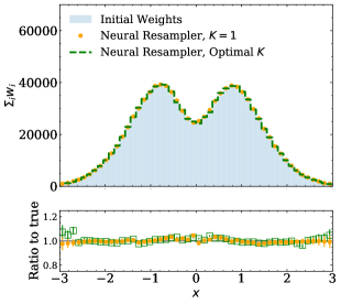
The weighted histogram of $X$ is shown by the blue solid distribution in Fig. 1a, corresponding to a Gaussian with a dip in the middle. After neural resampling with $K=1$, shown by the orange dotted curve, we obtain the same true distribution up to statistical fluctuations. As desired, subsampling with the optimal value of $K$ from Eq. (12) does not change the probability density, as shown by the green dashed curve. This subsampling does change the uncertainties, though, as discussed more below. We therefore conclude that neural resampling has successfully preserved the cross section via Eq. (2).

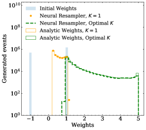
A nice feature of this example is that the correct unbinned weights are computable analytically using the asymptotic formulas in Sec. II. In Fig. 1b, we show the original weight distribution together with the positive neural resampling weights using both $K=1$ and the optimal value of $K$. While the original weights are both positive and negative, neural resampling yields strictly positive weights. We see that the finite sampling matches the expected analytic weight distributions, which is a non-trivial cross check of our neural reweighting code. Note that even though a binning and finite sampling are chosen to represent the data in Fig. 1a, all of these distributions are fundamentally unbinned.

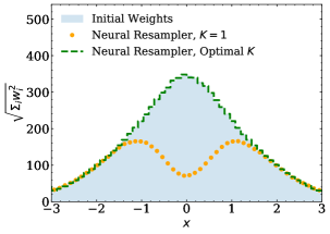
In Fig. 1c, we show the distribution of uncertainties using the standard Monte Carlo estimate based on summing the squared weights. With $K=1$, the uncertainties are substantially underestimated relative to the original distribution, especially in the vicinity of $x=0$, where there are large cancellations between negative and positive weights. Subsampling with the optimal $K$ restores the original uncertainties, as desired. We therefore conclude that neural resampling has successfully preserved the uncertainties via Eq. (5).

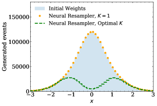
As shown in Fig. 1d, subsampling yields a significant savings in terms of the number of events required to obtain the same statistical properties as the original sample. Only one third of the events are needed to capture the same behavior of the original events, with the savings greatest near $x=0$ where there are larger relative uncertainties.

This two Gaussian example highlights the efficacy of neural resampling in a simple one-dimensional example. We now turn to a case of relevance to collider physics where the phase space is multi-dimensional.

IV.2 Top Quark Pair Production

(a)

(b)

(d)

Figure 2: Demonstration of neural resampling in a realistic collider example of top quark pair production at NLO matched to a parton shower. (a) The (rescaled) cross section for the leading ISR jet $p_{T}$. (b) The distribution of the event weights. The optimal $K$ spectrum steeply falls out to about 10, but the distribution is truncated at 4.5 to aid the comparison with the other histograms. (c) The (rescaled) uncertainties for $p_{T}$. (d) The number of events as a function of $p_{T}$. As in Fig. 1a, the curves correspond to (solid blue) the original event sample with positive and negative weights, (orange dotted) neural resampling with $K=1$, and (green dashed) neural resampling with the optimal $K$ value in Eq. (12).

      
      

(c)

(a)

(b)

(d)

Figure 3: The same as Fig. 2a, but now plotting the number of ISR jets with $p_{T}>10$ GeV. Note that the weight distribution in (b) is identical to Fig. 2b, since neural resampling acts on the full unbinned phase space.

      
      

(c)

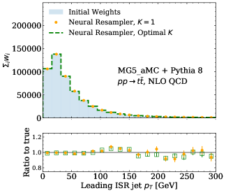
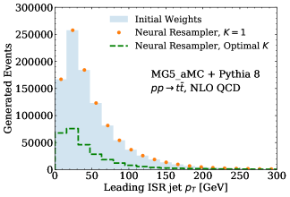
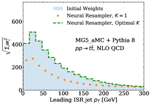
Our realistic collider case study is based on top quark pair production at NLO in quantum chromodynamics. At fixed order in an expansion in the strong coupling constant $\alpha_{s}$, it is well known that cross sections can become negative due to the breakdown of perturbation theory in the vicinity of soft/collinear singularities (see footnote 2). These unphysical phase space regions can be regulated by matching to a parton shower, rendering the differential cross section to be positive. In addition, matching improves the accuracy of the cross section prediction by including resummation effects beyond NLO.

The analysis below is based on 2M total events generated as follows. Fixed-order $t\bar{t}$ production is generated using MG5_aMC@NLO 5.2.7.2 Alwall et al. (2014) interfaced with the NNPDF 2.3 NLO parton density function set Ball et al. (2013). This fixed-order calculation uses MadLoop 2.7.2 Hirschi et al. (2011); Alwall et al. (2014), Ninja 1.2.0 Mastrolia et al. (2012); Peraro (2014), CutTools 1.9.3 Ossola et al. (2008), and OneLoop 3.6  van Hameren (2011); van Hameren et al. (2009). In these samples, the top quarks are forced to decay leptonically via $t\bar{t}\rightarrow b\bar{b}\mu^{+}\mu^{-}\nu\bar{\nu}$. Using the default FKS subtraction scheme Frixione et al. (1996); Frixione (1997), the resulting events are matched with the Pythia 8.230 Sjöstrand et al. (2015, 2006) parton shower, keeping the default shower settings. Initial state radiation (ISR) is generated both from the NLO calculation and from the subsequent parton shower matching.

The resulting events in the HepMC 2.06.09 Dobbs and Hansen (2000) format are processed with the HepMC reader module of Delphes 3.4.2 de Favereau et al. (2014). This setup is also used to cluster $R=0.4$ anti-$k_{t}$ jets Cacciari et al. (2012) with FastJet Cacciari and Salam (2006). Jets originating from a $b$-quark are identified as such using the flavor tagging module in Delphes. Jets are labeled as “ISR” if they are not $b$-jets. We suppress the overall cross section information and take the weights to be $\pm 1$. After neural resampling, it is straightforward to rescale all of the weights to have the proper dimensions of a cross section, but we elide this step for simplicity.

To implement neural resampling, we use PFNs Komiske et al. (2019), where each event is represented as a variable-length set of four-vectors that correspond to the muons, neutrinos, and clustered jets. The PdgID Tanabashi et al. (2018) of the muons and neutrinos are used as a per-particle feature in the PFN, while the $b$-jets (ISR jets) are given the per-particle feature of 1 (0). In principle, we could have applied neural resampling directly to the final-state hadrons, but since we are only going to plot jet-related quantities, it makes sense to perform jet clustering before neural resampling.

Note that the phase space that is being reweighted here is variable dimensional, with at least 20 dimensions from the 3-momenta for 6 particles and 2 jet masses. These data are constrained to an 18-dimensional manifold after considering transverse momentum conservation and are approximately constrained to a 14-dimensional manifold after accounting for mass-shell conditions. Many events have far more dimensions due to additional jets. Thus, this is a highly non-trivial test of whether neural resampling can yield sensible results across a multi-dimensional and variable-dimensional phase space.

In Fig. 2a, we plot the distribution of transverse momentum ($p_{T}$) of the leading ISR jet. As expected, neural resampling has matched the bulk of this distribution up to statistical uncertainties. In the tails, where training data are more sparse, there are larger variations, but we emphasize that these results were obtained “out of the box” with no attempt to optimize training parameters.

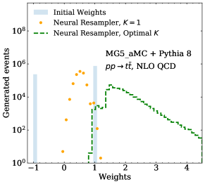
The distribution of event weights is shown in Fig. 2b. The original sample had both positive and negative weights, but neural resampling has yielded a positive weight distribution as desired. With the optimal choice of $K$, the event weights extend out to about 10, which reflects the initial inefficiency of event generation with positive and negative weights.

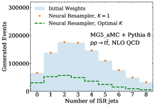
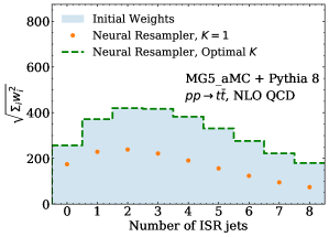
The uncertainties are shown in Fig. 2c, again using the standard Monte Carlo estimate from Eq. (5). With $K=1$, the uncertainties are underestimated throughout the phase space, but with the optimal value of $K$, they are captured correctly. Correspondingly, the optimal value of $K$ yields a substantially lower number of events, as shown in Fig. 2d, indicating a large gain in downstream computational efficiency. In particular, from the original 2M events, only about 600k remain after neural resampling, with no change to the statistical properties.

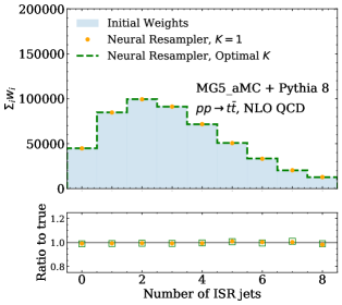
To highlight that neural resampling yields sensible results across the whole (unbinned) phase space, we plot the distribution of the number of ISR jets with $p_{T}$ $>$ 10 GeV in Fig. 3a. We emphasize that no retraining is needed here, since these plots are based on the same weights already shown in Fig. 2b. Obtaining results like this that work for any observable of interest would be challenging with a binned approach. This case study therefore suggests that neural reweighting will be a powerful tool for efficient use of Monte Carlo generators at colliders.

V Conclusions and Outlook

This paper has introduced neural resampling, a neural-network-based extension of the binned positive resampler proposed in Ref. Andersen et al. (2020). By exploiting the ability of neural networks to approximate likelihood ratios, our new approach is able to eliminate negative weights without binning and with access to potentially high-dimensional (and variable-sized) phase spaces. Furthermore, neural resampling preserves statistical uncertainties with minimal overhead and no adjustable parameters. This uncertainty preservation scheme is general and can also be applied to binned (non-neural network) resampling.

Given the growing availability of higher-order corrections and the computational demands of detector simulations, there is a need to make the best use of limited resources. The neural resampler is able to preserve the statistical power of these precision calculations while decreasing downstream computational demands. For the future, it would be interesting to study whether neural resampling could be incorporated more directly into the Monte Carlo generation process. This could lead to further computational gains, particularly if used in concert with emerging neural-network-based phase space integration techniques.

Beyond just computational efficiency, there may be other advantages of neural resampling. Many analysis strategies that consider the full unbinned log likelihood over events require per event weights to be positive Nachman (2020), which is guaranteed by neural resampling (assuming non-negative cross section). Monte Carlo generators increasingly have the ability to keep track of uncertainties via weight variations Mrenna and Skands (2016); Bothmann et al. (2016), which may be straightforward to incorporate into neural resampling via parametrized networks Baldi et al. (2016); Andreassen and Nachman (2020). Finally, neural resampling ensures that the event weights are a true function of phase space and not multivalued maps, even allowing the weight function to be differentiated. This feature of the learned weight function may turn out to be beneficial for other aspects of data processing and analysis.

Code and Data

The code for this paper can be found at https://github.com/bnachman/NeuralPositiveResampler. The top quark datasets are available upon request.

References

- Andersen et al. (2020) J. R. Andersen, C. Gutschow, A. Maier, and S. Prestel, A positive resampler for monte carlo events with negative weights, (2020), arXiv:2005.09375 [hep-ph] .
- Sjöstrand et al. (2015) T. Sjöstrand, S. Ask, J. R. Christiansen, R. Corke, N. Desai, P. Ilten, S. Mrenna, S. Prestel, C. O. Rasmussen, and P. Z. Skands, An Introduction to PYTHIA 8.2, Comput. Phys. Commun. 191, 159 (2015), arXiv:1410.3012 [hep-ph] .
- Bellm et al. (2016) J. Bellm et al., Herwig 7.0/Herwig++ 3.0 release note, Eur. Phys. J. C 76, 196 (2016), arXiv:1512.01178 [hep-ph] .
- Bothmann et al. (2019) E. Bothmann et al. (Sherpa), Event Generation with Sherpa 2.2, SciPost Phys. 7, 034 (2019), arXiv:1905.09127 [hep-ph] .
- Nason and Ridolfi (2006) P. Nason and G. Ridolfi, A Positive-weight next-to-leading-order Monte Carlo for Z pair hadroproduction, JHEP 08, 077, arXiv:hep-ph/0606275 .
- Frixione and Webber (2002) S. Frixione and B. R. Webber, Matching NLO QCD computations and parton shower simulations, JHEP 06, 029, arXiv:hep-ph/0204244 .
- Alwall et al. (2014) J. Alwall, R. Frederix, S. Frixione, V. Hirschi, F. Maltoni, O. Mattelaer, H. S. Shao, T. Stelzer, P. Torrielli, and M. Zaro, The automated computation of tree-level and next-to-leading order differential cross sections, and their matching to parton shower simulations, JHEP 07, 079, arXiv:1405.0301 [hep-ph] .
- Alioli et al. (2010) S. Alioli, P. Nason, C. Oleari, and E. Re, A general framework for implementing NLO calculations in shower Monte Carlo programs: the POWHEG BOX, JHEP 06, 043, arXiv:1002.2581 [hep-ph] .
- Agostinelli et al. (2003) S. Agostinelli et al. (GEANT4), GEANT4: A Simulation toolkit, Nucl. Instrum. Meth. A 506, 250 (2003).
- Albrecht et al. (2019) J. Albrecht et al. (HEP Software Foundation), A Roadmap for HEP Software and Computing R&D for the 2020s, Comput. Softw. Big Sci. 3, 7 (2019), arXiv:1712.06982 [physics.comp-ph] .
- Amoroso et al. (2020) S. Amoroso et al. (HSF Physics Event Generator WG), Challenges in Monte Carlo event generator software for High-Luminosity LHC, (2020), arXiv:2004.13687 [hep-ph] .
- Frederix et al. (2020) R. Frederix, S. Frixione, S. Prestel, and P. Torrielli, On the reduction of negative weights in MC@NLO-type matching procedures, (2020), arXiv:2002.12716 [hep-ph] .
- Cranmer et al. (2015) K. Cranmer, J. Pavez, and G. Louppe, Approximating Likelihood Ratios with Calibrated Discriminative Classifiers, (2015), arXiv:1506.02169 [stat.AP] .
- Brehmer et al. (2018a) J. Brehmer, K. Cranmer, G. Louppe, and J. Pavez, A Guide to Constraining Effective Field Theories with Machine Learning, Phys. Rev. D 98, 052004 (2018a), arXiv:1805.00020 [hep-ph] .
- Brehmer et al. (2018b) J. Brehmer, K. Cranmer, G. Louppe, and J. Pavez, Constraining Effective Field Theories with Machine Learning, (2018b), arXiv:1805.00013 [hep-ph] .
- Brehmer et al. (2020a) J. Brehmer, G. Louppe, J. Pavez, and K. Cranmer, Mining gold from implicit models to improve likelihood-free inference, Proc. Nat. Acad. Sci. , 201915980 (2020a), arXiv:1805.12244 [stat.ML] .
- Stoye et al. (2018) M. Stoye, J. Brehmer, G. Louppe, J. Pavez, and K. Cranmer, Likelihood-free inference with an improved cross-entropy estimator, (2018), arXiv:1808.00973 [stat.ML] .
- Andreassen and Nachman (2020) A. Andreassen and B. Nachman, Neural Networks for Full Phase-space Reweighting and Parameter Tuning, Phys. Rev. D 101, 091901 (2020), arXiv:1907.08209 [hep-ph] .
- Brehmer et al. (2020b) J. Brehmer, F. Kling, I. Espejo, and K. Cranmer, MadMiner: Machine learning-based inference for particle physics, Comput. Softw. Big Sci. 4, 3 (2020b), arXiv:1907.10621 [hep-ph] .
- Andreassen et al. (2020a) A. Andreassen, P. T. Komiske, E. M. Metodiev, B. Nachman, and J. Thaler, OmniFold: A Method to Simultaneously Unfold All Observables, Phys. Rev. Lett. 124, 182001 (2020a), arXiv:1911.09107 [hep-ph] .
- Andreassen et al. (2020b) A. Andreassen, B. Nachman, and D. Shih, Simulation Assisted Likelihood-free Anomaly Detection, Phys. Rev. D 101, 095004 (2020b), arXiv:2001.05001 [hep-ph] .
- Hollingsworth and Whiteson (2020) J. Hollingsworth and D. Whiteson, Resonance Searches with Machine Learned Likelihood Ratios, (2020), arXiv:2002.04699 [hep-ph] .
- Badiali et al. (2020) C. Badiali, F. Di Bello, G. Frattari, E. Gross, V. Ippolito, M. Kado, and J. Shlomi, Efficiency Parameterization with Neural Networks, (2020), arXiv:2004.02665 [hep-ex] .
- Komiske et al. (2019) P. T. Komiske, E. M. Metodiev, and J. Thaler, Energy Flow Networks: Deep Sets for Particle Jets, JHEP 01, 121, arXiv:1810.05165 [hep-ph] .
- Zaheer et al. (2017) M. Zaheer, S. Kottur, S. Ravanbakhsh, B. Poczos, R. R. Salakhutdinov, and A. J. Smola, Deep sets, in Advances in Neural Information Processing Systems 30, edited by I. Guyon, U. V. Luxburg, S. Bengio, H. Wallach, R. Fergus, S. Vishwanathan, and R. Garnett (Curran Associates, Inc., 2017) pp. 3391–3401.
- Goodfellow et al. (2014) I. J. Goodfellow, J. Pouget-Abadie, M. Mirza, B. Xu, D. Warde-Farley, S. Ozair, A. Courville, and Y. Bengio, Generative Adversarial Networks, (2014), arXiv:1406.2661 [stat.ML] .
- Kingma and Welling (2013) D. P. Kingma and M. Welling, Auto-Encoding Variational Bayes, arXiv e-prints , arXiv:1312.6114 (2013), arXiv:1312.6114 [stat.ML] .
- Jimenez Rezende et al. (2014) D. Jimenez Rezende, S. Mohamed, and D. Wierstra, Stochastic Backpropagation and Approximate Inference in Deep Generative Models, arXiv e-prints , arXiv:1401.4082 (2014), arXiv:1401.4082 [stat.ML] .
- de Oliveira et al. (2017a) L. de Oliveira, M. Paganini, and B. Nachman, Learning Particle Physics by Example: Location-Aware Generative Adversarial Networks for Physics Synthesis, Comput. Softw. Big Sci. 1, 4 (2017a), arXiv:1701.05927 [stat.ML] .
- Paganini et al. (2018a) M. Paganini, L. de Oliveira, and B. Nachman, Accelerating Science with Generative Adversarial Networks: An Application to 3D Particle Showers in Multilayer Calorimeters, Phys. Rev. Lett. 120, 042003 (2018a), arXiv:1705.02355 [hep-ex] .
- Paganini et al. (2018b) M. Paganini, L. de Oliveira, and B. Nachman, CaloGAN : Simulating 3D high energy particle showers in multilayer electromagnetic calorimeters with generative adversarial networks, Phys. Rev. D97, 014021 (2018b), arXiv:1712.10321 [hep-ex] .
- Alonso-Monsalve and Whitehead (2018) S. Alonso-Monsalve and L. H. Whitehead, Image-based model parameter optimization using Model-Assisted Generative Adversarial Networks 10.1109/TNNLS.2020.2969327 (2018), arXiv:1812.00879 [cs.CV] .
- Butter et al. (2019a) A. Butter, T. Plehn, and R. Winterhalder, How to GAN Event Subtraction, (2019a), arXiv:1912.08824 [hep-ph] .
- Arjona Martinez et al. (2019) J. Arjona Martinez, T. Q. Nguyen, M. Pierini, M. Spiropulu, and J.-R. Vlimant, Particle Generative Adversarial Networks for full-event simulation at the LHC and their application to pileup description (2019) arXiv:1912.02748 [hep-ex] .
- Bellagente et al. (2019) M. Bellagente, A. Butter, G. Kasieczka, T. Plehn, and R. Winterhalder, How to GAN away Detector Effects, (2019), arXiv:1912.00477 [hep-ph] .
- Vallecorsa et al. (2019) S. Vallecorsa, F. Carminati, and G. Khattak, 3D convolutional GAN for fast simulation, Proceedings, 23rd International Conference on Computing in High Energy and Nuclear Physics (CHEP 2018): Sofia, Bulgaria, July 9-13, 2018 214, 02010 (2019).
- Ahdida et al. (2019) C. Ahdida et al. (SHiP), Fast simulation of muons produced at the SHiP experiment using Generative Adversarial Networks, JINST 14, P11028, arXiv:1909.04451 [physics.ins-det] .
- Carrazza and Dreyer (2019) S. Carrazza and F. A. Dreyer, Lund jet images from generative and cycle-consistent adversarial networks, Eur. Phys. J. C79, 979 (2019), arXiv:1909.01359 [hep-ph] .
- Butter et al. (2019b) A. Butter, T. Plehn, and R. Winterhalder, How to GAN LHC Events, SciPost Phys. 7, 075 (2019b), arXiv:1907.03764 [hep-ph] .
- Lin et al. (2019) J. Lin, W. Bhimji, and B. Nachman, Machine Learning Templates for QCD Factorization in the Search for Physics Beyond the Standard Model, JHEP 05, 181, arXiv:1903.02556 [hep-ph] .
- Di Sipio et al. (2019) R. Di Sipio, M. Faucci Giannelli, S. Ketabchi Haghighat, and S. Palazzo, DijetGAN: A Generative-Adversarial Network Approach for the Simulation of QCD Dijet Events at the LHC, JHEP 08, 110, arXiv:1903.02433 [hep-ex] .
- Hashemi et al. (2019) B. Hashemi, N. Amin, K. Datta, D. Olivito, and M. Pierini, LHC analysis-specific datasets with Generative Adversarial Networks, (2019), arXiv:1901.05282 [hep-ex] .
- Chekalina et al. (2018) V. Chekalina, E. Orlova, F. Ratnikov, D. Ulyanov, A. Ustyuzhanin, and E. Zakharov, Generative Models for Fast Calorimeter Simulation.LHCb case (2018) arXiv:1812.01319 [physics.data-an] .
- ATL (2018) Deep generative models for fast shower simulation in ATLAS, ATL-SOFT-PUB-2018-001 (2018).
- Zhou et al. (2019) K. Zhou, G. Endrodi, L.-G. Pang, and H. Stocker, Regressive and generative neural networks for scalar field theory, Phys. Rev. D100, 011501 (2019), arXiv:1810.12879 [hep-lat] .
- Carminati et al. (2018) F. Carminati, A. Gheata, G. Khattak, P. Mendez Lorenzo, S. Sharan, and S. Vallecorsa, Three dimensional Generative Adversarial Networks for fast simulation, Proceedings, 18th International Workshop on Advanced Computing and Analysis Techniques in Physics Research (ACAT 2017): Seattle, WA, USA, August 21-25, 2017 1085, 032016 (2018).
- Vallecorsa (2018) S. Vallecorsa, Generative models for fast simulation, Proceedings, 18th International Workshop on Advanced Computing and Analysis Techniques in Physics Research (ACAT 2017): Seattle, WA, USA, August 21-25, 2017 1085, 022005 (2018).
- Datta et al. (2018) K. Datta, D. Kar, and D. Roy, Unfolding with Generative Adversarial Networks, (2018), arXiv:1806.00433 [physics.data-an] .
- Musella and Pandolfi (2018) P. Musella and F. Pandolfi, Fast and Accurate Simulation of Particle Detectors Using Generative Adversarial Networks, Comput. Softw. Big Sci. 2, 8 (2018), arXiv:1805.00850 [hep-ex] .
- Erdmann et al. (2018) M. Erdmann, L. Geiger, J. Glombitza, and D. Schmidt, Generating and refining particle detector simulations using the Wasserstein distance in adversarial networks, Comput. Softw. Big Sci. 2, 4 (2018), arXiv:1802.03325 [astro-ph.IM] .
- Deja et al. (2019) K. Deja, T. Trzcinski, and u. Graczykowski, Generative models for fast cluster simulations in the TPC for the ALICE experiment, Proceedings, 23rd International Conference on Computing in High Energy and Nuclear Physics (CHEP 2018): Sofia, Bulgaria, July 9-13, 2018 214, 06003 (2019).
- Derkach et al. (2019) D. Derkach, N. Kazeev, F. Ratnikov, A. Ustyuzhanin, and A. Volokhova, Cherenkov Detectors Fast Simulation Using Neural Networks (2019) arXiv:1903.11788 [hep-ex] .
- Erbin and Krippendorf (2018) H. Erbin and S. Krippendorf, GANs for generating EFT models, (2018), arXiv:1809.02612 [cs.LG] .
- Erdmann et al. (2019) M. Erdmann, J. Glombitza, and T. Quast, Precise simulation of electromagnetic calorimeter showers using a Wasserstein Generative Adversarial Network, Comput. Softw. Big Sci. 3, 4 (2019), arXiv:1807.01954 [physics.ins-det] .
- de Oliveira et al. (2017b) L. de Oliveira, M. Paganini, and B. Nachman, Tips and Tricks for Training GANs with Physics Constraints (2017).
- de Oliveira et al. (2018) L. de Oliveira, M. Paganini, and B. Nachman, Controlling Physical Attributes in GAN-Accelerated Simulation of Electromagnetic Calorimeters, J. Phys. Conf. Ser. 1085, 042017 (2018), arXiv:1711.08813 [hep-ex] .
- Farrell et al. (2019) S. Farrell, W. Bhimji, T. Kurth, M. Mustafa, D. Bard, Z. Lukic, B. Nachman, and H. Patton, Next Generation Generative Neural Networks for HEP, EPJ Web Conf. 214, 09005 (2019).
- Hooberman et al. (2017) B. Hooberman, A. Farbin, G. Khattak, V. Pacela, M. Pierini, J.-R. Vlimant, M. Spiropulu, W. Wei, M. Zhang, and S. Vallecorsa, Calorimetry with Deep Learning: Particle Classification, Energy Regression, and Simulation for High-Energy Physics (2017).
- Belayneh et al. (2019) D. Belayneh et al., Calorimetry with Deep Learning: Particle Simulation and Reconstruction for Collider Physics, (2019), arXiv:1912.06794 [physics.ins-det] .
- Buhmann et al. (2020) E. Buhmann, S. Diefenbacher, E. Eren, F. Gaede, G. Kasieczka, A. Korol, and K. Kruger, Getting High: High Fidelity Simulation of High Granularity Calorimeters with High Speed, (2020), arXiv:2005.05334 [physics.ins-det] .
- Albergo et al. (2019) M. S. Albergo, G. Kanwar, and P. E. Shanahan, Flow-based generative models for Markov chain Monte Carlo in lattice field theory, Phys. Rev. D100, 034515 (2019), arXiv:1904.12072 [hep-lat] .
- Kanwar et al. (2020) G. Kanwar, M. S. Albergo, D. Boyda, K. Cranmer, D. C. Hackett, S. Racaniere, D. J. Rezende, and P. E. Shanahan, Equivariant flow-based sampling for lattice gauge theory, (2020), arXiv:2003.06413 [hep-lat] .
- Urban and Pawlowski (2018) J. M. Urban and J. M. Pawlowski, Reducing Autocorrelation Times in Lattice Simulations with Generative Adversarial Networks, (2018), arXiv:1811.03533 [hep-lat] .
- Nicoli et al. (2020) K. A. Nicoli, C. J. Anders, L. Funcke, T. Hartung, K. Jansen, P. Kessel, S. Nakajima, and P. Stornati, On Estimation of Thermodynamic Observables in Lattice Field Theories with Deep Generative Models, (2020), arXiv:2007.07115 [hep-lat] .
- Ball et al. (2017) R. D. Ball et al. (NNPDF), Parton distributions from high-precision collider data, Eur. Phys. J. C 77, 663 (2017), arXiv:1706.00428 [hep-ph] .
- Carrazza and Cruz-Martinez (2019) S. Carrazza and J. Cruz-Martinez, Towards a new generation of parton densities with deep learning models, Eur. Phys. J. C 79, 676 (2019), arXiv:1907.05075 [hep-ph] .
- Bendavid (2017) J. Bendavid, Efficient Monte Carlo Integration Using Boosted Decision Trees and Generative Deep Neural Networks, (2017), arXiv:1707.00028 [hep-ph] .
- Klimek and Perelstein (2018) M. D. Klimek and M. Perelstein, Neural Network-Based Approach to Phase Space Integration, (2018), arXiv:1810.11509 [hep-ph] .
- Bothmann et al. (2020) E. Bothmann, T. Janßen, M. Knobbe, T. Schmale, and S. Schumann, Exploring phase space with Neural Importance Sampling, (2020), arXiv:2001.05478 [hep-ph] .
- Gao et al. (2020a) C. Gao, J. Isaacson, and C. Krause, i-flow: High-Dimensional Integration and Sampling with Normalizing Flows, (2020a), arXiv:2001.05486 [physics.comp-ph] .
- Gao et al. (2020b) C. Gao, S. Höche, J. Isaacson, C. Krause, and H. Schulz, Event Generation with Normalizing Flows, Phys. Rev. D 101, 076002 (2020b), arXiv:2001.10028 [hep-ph] .
- Bishara and Montull (2019) F. Bishara and M. Montull, (Machine) Learning Amplitudes for Faster Event Generation, (2019), arXiv:1912.11055 [hep-ph] .
- Badger and Bullock (2020) S. Badger and J. Bullock, Using neural networks for efficient evaluation of high multiplicity scattering amplitudes, (2020), arXiv:2002.07516 [hep-ph] .
- Monk (2018) J. W. Monk, Deep Learning as a Parton Shower, (2018), arXiv:1807.03685 [hep-ph] .
- Andreassen et al. (2019a) A. Andreassen, I. Feige, C. Frye, and M. D. Schwartz, Binary JUNIPR: an interpretable probabilistic model for discrimination, Phys. Rev. Lett. 123, 182001 (2019a), arXiv:1906.10137 [hep-ph] .
- Andreassen et al. (2019b) A. Andreassen, I. Feige, C. Frye, and M. D. Schwartz, JUNIPR: a Framework for Unsupervised Machine Learning in Particle Physics, Eur. Phys. J. C 79, 102 (2019b), arXiv:1804.09720 [hep-ph] .
- Chollet (2017) F. Chollet, Keras, https://github.com/fchollet/keras (2017).
- Abadi et al. (2016) M. Abadi, P. Barham, J. Chen, Z. Chen, A. Davis, J. Dean, M. Devin, S. Ghemawat, G. Irving, M. Isard, et al., Tensorflow: A system for large-scale machine learning., in OSDI, Vol. 16 (2016) pp. 265–283.
- Kingma and Ba (2014) D. Kingma and J. Ba, Adam: A method for stochastic optimization, (2014), arXiv:1412.6980 [cs] .
- Ball et al. (2013) R. D. Ball et al., Parton distributions with LHC data, Nucl. Phys. B 867, 244 (2013), arXiv:1207.1303 [hep-ph] .
- Hirschi et al. (2011) V. Hirschi, R. Frederix, S. Frixione, M. V. Garzelli, F. Maltoni, and R. Pittau, Automation of one-loop QCD corrections, JHEP 05, 044, arXiv:1103.0621 [hep-ph] .
- Mastrolia et al. (2012) P. Mastrolia, E. Mirabella, and T. Peraro, Integrand reduction of one-loop scattering amplitudes through Laurent series expansion, JHEP 06, 095, [Erratum: JHEP 11, 128 (2012)], arXiv:1203.0291 [hep-ph] .
- Peraro (2014) T. Peraro, Ninja: Automated Integrand Reduction via Laurent Expansion for One-Loop Amplitudes, Comput. Phys. Commun. 185, 2771 (2014), arXiv:1403.1229 [hep-ph] .
- Ossola et al. (2008) G. Ossola, C. G. Papadopoulos, and R. Pittau, CutTools: A Program implementing the OPP reduction method to compute one-loop amplitudes, JHEP 03, 042, arXiv:0711.3596 [hep-ph] .
- van Hameren (2011) A. van Hameren, OneLOop: For the evaluation of one-loop scalar functions, Comput. Phys. Commun. 182, 2427 (2011), arXiv:1007.4716 [hep-ph] .
- van Hameren et al. (2009) A. van Hameren, C. Papadopoulos, and R. Pittau, Automated one-loop calculations: A Proof of concept, JHEP 09, 106, arXiv:0903.4665 [hep-ph] .
- Frixione et al. (1996) S. Frixione, Z. Kunszt, and A. Signer, Three jet cross-sections to next-to-leading order, Nucl. Phys. B 467, 399 (1996), arXiv:hep-ph/9512328 .
- Frixione (1997) S. Frixione, A General approach to jet cross-sections in QCD, Nucl. Phys. B 507, 295 (1997), arXiv:hep-ph/9706545 .
- Sjöstrand et al. (2006) T. Sjöstrand, S. Mrenna, and P. Z. Skands, PYTHIA 6.4 Physics and Manual, JHEP 05, 026, arXiv:hep-ph/0603175 [hep-ph] .
- Dobbs and Hansen (2000) M. Dobbs and J. B. Hansen, The HepMC C++ Monte Carlo Event Record for High Energy Physics, Tech. Rep. ATL-SOFT-2000-001 (CERN, Geneva, 2000) revised version number 1 submitted on 2001-02-27 09:54:32.
- de Favereau et al. (2014) J. de Favereau, C. Delaere, P. Demin, A. Giammanco, V. Lemaître, A. Mertens, and M. Selvaggi (DELPHES 3), DELPHES 3, A modular framework for fast simulation of a generic collider experiment, JHEP 02, 057, arXiv:1307.6346 [hep-ex] .
- Cacciari et al. (2012) M. Cacciari, G. P. Salam, and G. Soyez, FastJet User Manual, Eur. Phys. J. C72, 1896 (2012), arXiv:1111.6097 [hep-ph] .
- Cacciari and Salam (2006) M. Cacciari and G. P. Salam, Dispelling the myth for the jet-finder, Phys. Lett. B641, 57 (2006), arXiv:hep-ph/0512210 [hep-ph] .
- Tanabashi et al. (2018) M. Tanabashi et al. (Particle Data Group), Review of particle physics, Phys. Rev. D 98, 030001 (2018).
- Nachman (2020) B. Nachman, A guide for deploying Deep Learning in LHC searches: How to achieve optimality and account for uncertainty, SciPost Phys. 8, 090 (2020), arXiv:1909.03081 [hep-ph] .
- Mrenna and Skands (2016) S. Mrenna and P. Skands, Automated Parton-Shower Variations in Pythia 8, Phys. Rev. D94, 074005 (2016), arXiv:1605.08352 [hep-ph] .
- Bothmann et al. (2016) E. Bothmann, M. Schönherr, and S. Schumann, Reweighting QCD matrix-element and parton-shower calculations, Eur. Phys. J. C76, 590 (2016), arXiv:1606.08753 [hep-ph] .
- Baldi et al. (2016) P. Baldi, K. Cranmer, T. Faucett, P. Sadowski, and D. Whiteson, Parameterized neural networks for high-energy physics, Eur. Phys. J. C76, 235 (2016), arXiv:1601.07913 [hep-ex] .