A fixed point for black hole distributions

Abstract

Understanding distributions of black holes is crucial to both astrophysics and quantum gravity. Studying astrophysical population statistics has even been suggested as a channel to constrain black hole formation from the quantum vacuum. Here we propose a Gedankenexperiment to show that the non-linear properties of binary mergers (simulated with accurate surrogate models) generate an attractor in the space of distributions. Our results show that the joint distribution of spin magnitude and fractional mass loss evolves to a fixed point, converging in a few generations. The features of this fixed point distribution do not depend on the choice of initial distribution. Since a black hole merger is irreversible it produces entropy – possibly the largest source of entropy in the universe. The fixed-point distributions are neither isothermal nor isentropic, and initially thermodynamic states evolve away from thermality. We finally evaluate the specific entropy production rate per merger from initially thermal and non-thermal distributions, which converges to a constant.

I Introduction

Black hole distribution functions carry a wealth of information, both in the theoretical context of quantum gravity, and the observational context of astrophysics. Since the work of Bekenstein and Hawking Bekenstein (1973, 1974, 1975); Hawking (1975), the interpretation of black holes as thermodynamic and statistical mechanical systems has established black holes as a key to understanding quantum gravity. Their thermal properties have lent weight to top-down calculations of the microscopic degrees of freedom of quantum gravity Strominger and Vafa (1996); Ashtekar et al. (1998). Meanwhile, in an astrophysical context, BH distribution functions teach us about stellar populations, the environments in which stars live, die, and give birth to BHs; dynamical interactions, and more Fryer and Kalogera (2001); Berti and Volonteri (2008); Gerosa et al. (2018); Kimball et al. (2019, 2020); Gerosa and Berti (2019); Rodriguez et al. (2019); Banerjee (2020). The possibility of primordial BHs (PBHs) lie at the intersection of quantum gravity and astrophysics. If they exist, their population may be an important component of dark matter, a question which can now be addressed with observations from Advanced LIGO and Virgo Carr and Kuhnel (2020). The quantum-mechanical and statistical properties of PBHs may leave imprints on astrophysical observations Raccanelli et al. (2018). Conversely, observations could test whether PBHs were seeded by a quantum thermodynamic process, producing PBHs in a (micro)canonical ensemble Bianchi et al. (2018).

In this paper, we present a fundamental black hole distribution function, determined solely by the non-linear, irreversible, out-of-equilibrium process of the merger of two black holes. Binary black hole (BBH) mergers are the dominant source in gravitational-wave astronomy Abbott et al. (2016, 2017a, 2017b, 2019a, 2019b, 2020), which enables the observational study of black hole distributions. Numerical relativity (NR) simulations Boyle et al. (2019) are necessary for modeling gravitational waveforms from binary black hole (BBH) mergers. However, NR simulations require substantial computational power and time to produce accurate results, which is an obstacle when spanning the whole seven-dimensional parameter space of quasicircular BBH mergers. Surrogate models Varma et al. (2019a, b) interpolate NR simulation data to compute both the gravitational waveform and the properties of the black hole remnant at points in parameter space even where no NR simulations were performed. These models are efficient enough to evaluate populations of thousands of BBH mergers in seconds on laptop/desktop computers.

We pioneer the use of surrogates to study black hole distribution functions. We simulate a thought experiment on a large population of black holes, where we choose initial spin and mass distributions. From this initial population, we configure a set of binaries by randomly resampling for BH pairs, and then allowing each pair to merge. The only condition we require is that the mass ratio of each binary is in the interval $1\leq q\leq 6$, where the results of the NRSur7dq4Remnant surrogate have been validated Varma et al. (2019b). We compute both the mass and the spin of each of the remnant black holes in the post-merger population using the surrogate model, rather than semiempirical expressions or analytical/numerical kludges Tichy and Marronetti (2008); Barausse et al. (2012); Hofmann et al. (2016); Gerosa and Kesden (2016); Campanelli et al. (2007); Gonzalez et al. (2007); Lousto and Zlochower (2008); Lousto et al. (2012); Lousto and Zlochower (2013). We then consider the remnant parameter distributions as new initial conditions for the next iteration to repeat this procedure, again resampling for binaries merging them, and find the mass and spin of every remnant in the next generation of black holes. Hence it is possible to visualize how the spin and mass distributions change with the number of generations. Our results show the distributions of spin magnitudes and relative mass ratios converge to fixed-point functions after a few generations. We quantitatively test for convergence using the Kullback-Leibler (KL) divergence Kullback and Leibler (1951) in the 2D distributions, finding that (a) our sampled distributions are consistent with being drawn from the same underlying continuous distribution; and (b) different choices of initial mass distributions only affect the number of generations needed to converge.

Figure 1: Left: Preparation of initial conditions from distributions of spins and masses. We assume an isotropic collection of black holes, meaning the spins are distributed uniformly in solid angle. Right: Resampling for pairs of black holes to merge, the outcome giving a subsequent generation of black holes. From a finite sample of BHs, we can randomly form $N_{\text{samp}}$ binaries (each BH chosen independently) to generate another $N_{\text{samp}}$ remnant BHs for the next generation. The “box” prepared in the left panel is the same as the box on the top of the right panel, providing initial conditions for the first generation of mergers.

Some initial distribution functions are motivated probabilistically or astrophysically. Meanwhile, the Bekenstein-Hawking (BH) formulae for entropy and temperature Bekenstein (1973); Hawking (1975) for the Kerr solution allow us to define a population of black holes at constant temperature (or entropy). These distributions define isothermal (isentropic) curves in the mass-spin plane, similar to isothermal (isentropic) curves in a PV phase diagram for a gas in classical thermodynamics. After computing the mass and spin of remnant black holes for a few generations of binary mergers, we find that resulting generations are not constant temperature (entropy). This is due to the irreversibility and out-of-equilibrium dynamics of the highly non-linear merger process. Knowing the mass and spin of each remnant black hole, we can compute the entropy production rate of the distribution in each generation. Our results show that the specific entropy produced per merger is constant after a certain number of generations, depending on the shape of the initial mass distribution. This disfavors the presence of memory (in the Markov sense, not the BMS sense) in late-generation mergers.

The layout of this paper is as follows: in Section II, we describe in full detail the setup of our thought experiment. In Section III, we use the setup described in the previous section to show the existence of attractors in distribution space. We find that arbitrary distributions of mass and spin in a large population of black holes converge to fixed-point distributions of spin magnitude and relative mass ratios. For consistency, we use the Kullback-Leibler divergence to show that the distributions require a few generations to converge. The number of generations depends on the shape of the initial mass distribution. In Section IV, we evaluate the evolution of samples of black holes at constant Hawking temperature (entropy) forming an isothermal (isentropic) state. After successive binary mergers, we observe that the out-of-equilibrium, non-linear nature of the merging process suppresses the thermal features of such configurations. We also compute the entropy production rate per merger. We discuss and conclude in Section V.

II The thought experiment

Here we describe the setup of our proposed thought experiment to study the flow of distributions over merger generations. The surrogate model we use Varma et al. (2019b) is built on a seven-dimensional parameter space, consisting of two 3-D spin vectors and the mass ratio $q$. This model was trained on NR simulations in the range of mass-ratio spanning $1\leq q\leq 4$, while faithfully extending up to $q\leq 6$ by extrapolation. For dimensionless spin magnitudes $\chi=|\vec{\chi}|$, the model was built in the range $0\leq\chi\leq 0.8$, and extrapolates reasonably up to $\chi\leq 1.0$. As shown in Varma et al. (2019b) (cf. Figs. 10 and 11), the surrogate code is more precise than other validated fits such as SEOBNRv3. Going to more extreme mass ratios would require either semianalytical models Hughes and Blandford (2003); Barausse et al. (2012); Hofmann et al. (2016); Gerosa and Kesden (2016); Campanelli et al. (2007); Gonzalez et al. (2007); Lousto and Zlochower (2008); Lousto et al. (2012); Lousto and Zlochower (2013) or a new surrogate built in the style of Rifat et al. (2020). However, such models have not been validated against NR simulations at higher mass-ratios, e.g. SEOBNRv3 has been validated up to $q=5$ Babak et al. (2017).

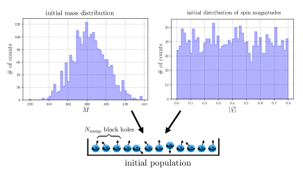
The limitations of NRSur7dq4Remnant inform what choices we can make for initial distributions. We select an initial population of black holes by assigning a mass $M$ and dimensionless spin vector $\vec{\chi}$ to each, sampled from a given distribution function, as shown in the left panel of Fig. 1. We assume spin direction is isotropically distributed, while spin magnitude is uniform in $\chi$. Since the surrogate model has a constraint on the mass ratio and spin magnitudes, we are constrained in our initial mass and spin distributions.

Figure 2: Evolution of the joint distribution $p(\mu_{\mathrm{rel}},\chi)$. The solid contours enclose 30%, 68%, and 95% of the probability mass of the $n$th generation. Dashed contours are from the fixed-point distribution. Each cross in the orange diffuse cloud represents a remnant black hole.

Figure 3: Evolution of the marginalized mass (left) and spin (right) distributions with generation. The initial conditions were a Kroupa mass distribution, and uniform in the magnitude $\chi$. The mass distribution gets narrower (in log space) with the number of generations. There is no noticeable difference in marginalized spin distribution from the third to the fifth generation, consistent with approaching the attractor distributions.

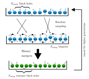
Once we choose initial distribution functions, we randomly sample $2N_{\text{samp}}$ BHs, grouped into $N_{\text{samp}}$ binaries, as depicted in the right panel of Fig. 1. After the coalescences, these samples generate a new population (colored in green) containing $N_{\text{samp}}$ first-generation black holes with remnant spins $\chi_{\text{fin}}$ and masses $M_{\text{fin}}$ provided by the surrogate code. We keep the resulting mass-spin correlation, which propagates to later generations, by taking the $N_{\text{samp}}$ samples of $(M_{\text{fin}},\chi_{\text{fin}})$ for each remnant to be the next generation. We however discard the remnant spin direction. The next step is to randomly resample (possibly with repetition) another $2N_{\text{samp}}$ black holes into pairs, which will participate in the next generation of mergers. We assume isotropy and thus randomize the spin direction of each black hole sample. These pairs are then merged, allowing the scheme to iterate for as many generations as desired.

Let us mention that recent research Abbott et al. (2019b); Gerosa and Berti (2019); Fishbach and Holz (2020) considers selective pairings (instead of treating each BH as independent), determined by a joint probability distribution $p(M_{1},M_{2})$. Present constraints on selective pairing are consistent with each mass being selected independently Abbott et al. (2019b), so we do not include this in our models, leaving it as a topic for future study. We must also add the caveat that astrophysically, BH binaries reside in stellar clusters or galaxies, and the GW kick at merger can unbind the remnant from the host. Such a kicked remnant would not make it into the next generation of merging BHs. We ignore this effect in our gedankenexperiment, because we are only interested in the invariant distribution determined by the merger dynamics, unaffected by astrophysical environments. Further, we do not model the more realistic scenario where BHs from multiple generations coexist in a common environment. We only model the transition from one generation to the next, using the generation index as a “time” variable, to understand the flow of the probability distribution functions.

Figure 4: Evolution of the cumulative relative mass ratio distribution $P(\mu_{\mathrm{rel}}<\mu)$ (left) and spin magnitude distribution $P(|\vec{\chi}|<\chi)$ (right) as a function of number of generations. The initial mass distribution was the Kroupa power law, for which it takes six generations to converge to the fixed-point. We plot the first four generations with dashed lines.

Figure 5: The cumulative distribution function of $\mu_{\mathrm{rel}}$ is independent of initial conditions. The same independence applies to the spin magnitude and the kick velocity distributions.

III Fixed-point distributions

We now show the evolution of populations with isotropic spins and different initial mass distributions converging to a fixed-point distribution. We sampled from a Gaussian, a log-normal, and a power-law distribution to simulate a population of $N_{\text{samp}}=$ 2000 black holes. The fixed point is a joint distribution in spin magnitude and relative mass ratio. We define the relative mass ratio $\mu_{\mathrm{rel}}$ as

$$\mu_{\mathrm{rel}}\equiv\frac{M_{\mathrm{fin}}}{M_{\mathrm{ini}}}\,,$$ (1)

where $M_{\mathrm{fin}}$ is the mass of the black hole remnant and $M_{\mathrm{ini}}\equiv M_{1}+M_{2}$ is the total mass of the progenitors. The fraction $1-\mu_{\mathrm{rel}}$ gives the ratio of emitted energy compared to the total initial mass of the binary.

In the case of the power-law distribution, we used $p(m)\propto m^{-2.3}$ corresponding to the initial Kroupa mass function Kroupa (2001); Gerosa and Berti (2017, 2019); Gerosa et al. (2020). In this scenario, we restrict the mass interval to $M\in[8;48]M_{\odot}$. This restriction is necessary since the applicability of NRSur7dq4Remnant has only been validated up to $1\leq q\leq 6$.

Figure 6: Evolution of mass distribution, with a log-normal initial condition. Each generation’s shape is consistent with log-normal. The evolution from an initial Gaussian is similar.

Figure 7: Values of $D_{\text{KL}}$ between 2D joint PDFs from adjacent generations, $D_{\text{KL}}(i+1||i)$, (red); or the PDF of generation $i$ relative to the last (19th) generation, $D_{\text{KL}}(19||i)$, (blue). Each dashed region contains the points needed to converge to a joint fixed-point distribution. Error bars are estimates of KDE finite sampling effects, estimated by subsampling 50% of the $N_{\text{samp}}=40,000$ binaries in each generation several times, and computing the variance. Left: Initial conditions are a Gaussian in mass. It only takes two generations to converge to a fixed-point distribution. Right: Initial conditions are a Kroupa power-law in mass. Here it takes at least seven or eight generations to converge to the same fixed-point distribution.

In Fig. 2 we show convergence to the attractive fixed-point distribution, starting from the Kroupa initial mass distribution and uniform in spin on the interval $\chi\sim\mathcal{U}[0.0;0.8]$. Solid contours contain 30%, 68%, and 95% of the probability mass, overplotted with dashed contours from the last generation. We can see that it takes five or six generations to converge. Now we would like to quantify the convergence. We use the Kullback-Leibler (KL) divergence Kullback and Leibler (1951) to measure how similar are the distributions at different generations, without marginalizing away any correlations.

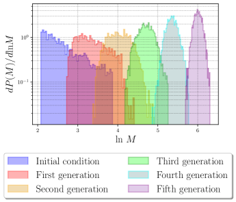
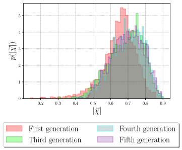
In Fig. 3, we show the evolution of the marginalized mass and spin magnitude distributions, from the same initial conditions. In the left panel, we see the mass distribution shifts to the right as black hole masses increase through mergers. Although the standard deviation of the mass distribution grows, the ratio between the largest and the smallest mass in the population tends to decrease. In the right panel, it is hard to distinguish between the probability densities $p(\chi)$ from the third generation onwards, evidence supporting the convergence to a fixed-point distribution. That the spin magnitude distribution peaks around $\chi\approx 0.7$ has also been observed before in Gerosa and Berti (2017); Fishbach et al. (2017), using approximate analytical models (and in an astrophysical setting). This even goes all the way back to the first successful BBH merger simulations Pretorius (2005). This is essentially a conversion of the orbital angular momentum of the two black holes, at the time of plunge, to the spin angular momentum of the remnant.

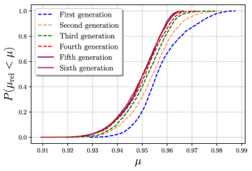
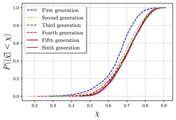
Convergence is more easily seen and can be tested robustly using cumulative distribution functions (CDFs). In Fig. 4, we depict in the left panel the evolution of the first six generations of the $\mu_{\mathrm{rel}}$ CDF. It immediately follows that the fraction of energy emitted also converges to a fixed-point distribution. We show the spin magnitude CDF in the right panel.

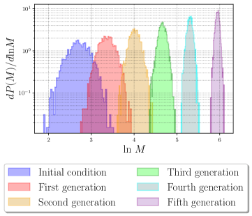
The distribution of the total BH mass tends to get narrower (in log space) as the number of generations increases, as it loses its memory of the initial distribution. Most changes in the shape of the mass and spin distributions can be quantified more precisely by measuring moments, as reported in Appendix B.

The Kullback-Leibler divergence, or relative entropy, is given by Kullback and Leibler (1951)

$$D_{\text{KL}}(p||q)\equiv\displaystyle{\int}p(x)\log_{2}\frac{p(x)}{q(x)}dx\,,$$ (2)

and is a measure of similarity between two probability distributions $p(x)$ and $q(x)$. It can be interpreted as the bits of information learned when updating prior $q(x)$ to posterior $p(x)$. In the case we study, the parameter space is two-dimensional and is made from the pairs $x=(\mu_{\mathrm{rel}},\chi)$. To estimate the integral above, we used a Gaussian kernel density estimator (KDE) implemented in the scipy.stats package Virtanen et al. (2020), and to minimize KDE noise, we used a population of size $N_{\text{samp}}=40,000$.

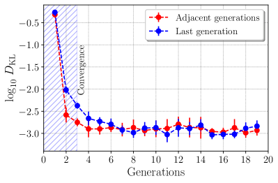
We computed $D_{\text{KL}}$ for joint PDFs from (a) adjacent generations, $D_{\text{KL}}(i+1||i)$, and (b) the $i$th and the last (19th) generation, $D_{\text{KL}}(19||i)$. We plot these values in Fig. 7, using the simulations initialized with a Gaussian mass distribution in the left panel. In both the adjacent (case a, red) and last (case b, blue) curves, there are only two points visible in the dashed rectangle before converging to a small value of $D_{\text{KL}}$, approximately $10^{-3}$ bits of relative entropy. We used bootstrapping to check that this value is consistent with sampling from a single underlying distribution. Thus, we only need two or three iterations for the distributions to become consistent with the fixed-point.

Figure 8: Left: Evolution of an isothermal collection of black holes. Right: Evolution of an isentropic collection of black holes. All the elements in the initial configuration belong to a constant temperature/entropy curve. In later generations, irreversible non-linear dynamics dilutes the thermal properties of the configurations, no longer on isothermal/isentropic curves, and they approach the fixed point distribution.

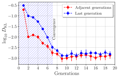
In the right panel of Fig. 7, we use the Kroupa power-law distribution as an initial configuration (individual PDFs and CDFs were in Figs. 3 and 4). Here we see the first seven generations in the dashed region in the left necessary to converge to a fixed value of $D_{\mathrm{KL}}$, consistent with a gain of almost zero bits for the two forms of comparison shown in the red and blue curves. Convergence is essentially equivalent if using another late generation (excluding those in the dashed regions in Fig. 7) as a representative of the fixed-point distribution instead of the 19th generation.

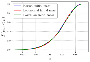
All three choices of initial mass distributions (Gaussian, log-normal, and Kroupa) converge to the same fixed point, as seen in Fig. 5. Similarly, other initial choices of $p(\chi)$ converge to the same fixed point distribution. The only difference, as seen in Fig. 7, is how many generations it takes to converge. As seen in the left panel of Fig. 3, the mass distribution approaches a centrally-peaked distribution. Therefore the initial Gaussian and log-normal converge more quickly than the Kroupa power law. Starting with a log-normal distribution shows an interesting feature, which can be seen in Fig. 6. Each generation is close to being log-normally distributed. That is, merging log-normally distributed masses generates remnants with masses that are also drawn from a (different) log-normal distribution.

IV Thermodynamics of distributions

Now we turn to the entropy production and thermal properties (or lack thereof) of these distributions, using the same setup as described in Sec. II. We are interested in the fundamental Bekenstein-Hawking properties Bekenstein (1973); Hawking (1975), rather than e.g. the kinetic temperature due to motion in a cluster or galaxy. Thus we use the formulas for the Kerr black hole,

$$\frac{T_{\mathrm{BH}}}{T_{H,\odot}} =\frac{M_{\odot}}{4\pi M}\frac{\sqrt{1-\chi^{2}}}{1+\sqrt{1-\chi^{2}}}\,,$$ (3)

$$\frac{S_{\mathrm{BH}}}{S_{H,\odot}} =\frac{\pi M^{2}}{M_{\odot}^{2}}\left(1+\chi^{2}+\sqrt{1-\chi^{2}}\right)\,,$$ (4)

which are in terms of the Bekenstein-Hawking temperature and entropy scaled by the quantities $T_{H,\odot}\equiv\hbar c^{3}/2Gk_{\mathrm{B}}M_{\odot}$ and $S_{H,\odot}\equiv 4GM^{2}_{\odot}/\hbar c$.

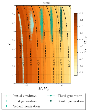
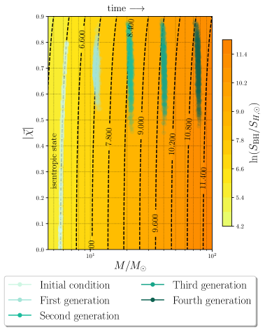
With these thermodynamic relations, we can sample black holes from various underlying distributions. Bianchi et al. Bianchi et al. (2018) considered sampling from a microcanonical ensemble, though early-universe fluctuations would arguably draw $(M,\chi)$ from a canonical ensemble (i.e. at fixed temperature) instead. This is possible, but the induced distribution on mass ratio has substantial weight outside of the range $1\leq q\leq 6$ that we need to apply the surrogate. We leave this for future work. Instead, we fix the same uniform spin distribution as before, and use Eqs. (3) and (4) as constraints for sampling at fixed temperature or entropy. With this approach, all of our initial configurations satisfy the mass-ratio constraint. We emphasize that none of our results change qualitatively if we select other ways to distribute spin magnitude. In Fig. 8, we show the evolution of the isothermal/isentropic states by plotting all the distributions in a mass/spin phase diagram, analogous to a pressure/volume diagram in ideal gas thermodynamics. In the left panel, we show the evolution of an initially isothermal configuration built from a uniformly distributed set of spin magnitudes. Isothermal states immediately evolve into non-thermal distributions, which do not follow constant temperature curves. In agreement with Eqs. (3) and (4), the temperature decreases as every black hole in the population becomes more massive. The same departure from thermality occurs with an initially isentropic state depicted in the right panel of this figure. Similarly entropy increases, since the remnants have increased area relative to the initial BHs. Departure from thermality is due to the highly non-linear dynamics of the merger process. A merger is irreversible, due to the area increase theorem, so entropy is generated. Furthermore a merger is not quasistatic, so horizon temperature need not even be well-defined throughout.

Figure 9: Evolution of the entropy production rate per merger for different choices of initial distributions. This quantity converges more slowly when the initial mass distribution is the Kroupa power law.

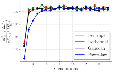
We can compute the entropy production simply via $\Delta S=S_{\text{fin}}-S_{\text{ini}}$. Notice that the dimensionless entropy production depends on mass ratio as

$$\frac{\Delta S}{M_{\mathrm{ini}}^{2}}\sim\frac{q}{(1+q)^{2}}\,,$$ (5)

where we ignored spin factors of order 1 and dimensionful constants like $k_{B}$. This shows that the entropy production peaks around $q\sim 1$ and is suppressed at extreme mass ratios. Therefore, our use of the surrogate model (with mass-ratio restricted to $1\leq q\leq 6$) does not degrade our calculation of entropy production.

We show the evolution of the entropy production rate per merger in Fig. 9, for different choices of the initial mass distributions. It is interesting to observe that the growth is slower when we use the Kroupa power-law distribution. This distribution takes up to five or six generations to converge, about the same number of generations as seen in Sec. III for convergence to the fixed-point distributions $p(\mu_{\mathrm{rel}},\chi)$. For each initial condition, we see that the entropy production grows until it reaches an approximately constant value. The isothermal, isentropic, log-normal, and Gaussian initial conditions all behave similarly. In all the cases we studied, once the system has converged to a fixed value for the entropy production, it seems to have lost any memory of the initial conditions.

Black holes are by far the most entropic systems in the universe Carroll and Chen (2004); Egan and Lineweaver (2010), and thus BBH mergers are the largest contributors to the entropy increase of the universe. The entropy production rate in Fig. 9 allows us to estimate the entropy production in the universe at redshift $z$, based on the BBH merger rate. Let $\mathcal{R}$ be the differential BBH merger rate, which depends on redshift and in principle on intrinsic parameters $\zeta\equiv(M_{\text{ini}},q,\vec{\chi}_{1},\vec{\chi}_{2})$ (in the notation of Ref. Abbott et al. (2019b)),

$$\mathcal{R}(z,\zeta)=\frac{dN}{dt\,dV\,d\zeta}\,.$$ (6)

Then in principle, the entropy production rate due to BBH mergers is

$$\frac{dS}{dt}(z)=\int\Delta S(\zeta)\mathcal{R}(z,\zeta)\,dV\,d\zeta\,.$$ (7)

We have argued in Eq. (5) that $\Delta S$ peaks at mass ratios close to 1, as does $\mathcal{R}$, based on astronomical observations. Thus as an approximation, using the value from Fig. 9, the entropy production rate is

$$\frac{dS}{dt}\approx\int 1.35\pi S_{H,\odot}\left(\frac{M_{\mathrm{ini}}}{M_{\odot}}\right)^{2}R(z,M_{\text{ini}})\,dVdM_{\text{ini}}\,,$$ (8)

where $R=dN/(dt\,dV\,dM_{\text{ini}})$, we have taken the average over spins, and assumed the integral is dominated around $q\approx 1$. The integrated and mass-differential merger rate has been inferred for stellar mass BHs from Advanced LIGO and Virgo observations Abbott et al. (2019b). The SMBH merger rate is currently unknown, but can be estimated from cosmological simulations Rodriguez-Gomez et al. (2015). Future PTA observations may infer this rate, and currently provide upper limits Arzoumanian et al. (2018); Chen et al. (2019). These limits can not yet say if the entropy production is dominated by stellar mass or supermassive BBHs.

V Discussion

In this paper, we conducted a gedankenexperiment to study the evolution of black hole distributions, due only to the intrinsic non-linear dynamics of binary mergers. Our main finding is the existence of an attractive fixed-point distribution in the space of spin magnitude $\chi$ and relative mass ratio $\mu_{\text{rel}}$ (or fraction of mass retained). We used the surrogate routines in NRSur7dq4Remnant to compute the remnant mass and spin of each merger in the population after every iteration/generation. Although we used stellar-mass scale black holes as examples in this work, the thought experiment itself is scale-free: it can extend up to supermassive black holes or down to primordial ones. Our interest is in the underlying fixed-point distribution due to merger dynamics, so we did not attempt to capture real astrophysical effects like unbinding from a cluster or galactic halo.

All initial distributions we studied (Gaussian, log-normal, Kroupa, isothermal, isentropic) converged to the same fixed point distribution. The only difference was the number of generations needed for convergence. We quantified this convergence with the Kullback-Leibler divergence.

We studied the (lack of) thermality of the fixed-point distribution, from the point of view of black hole thermodynamics. Starting with states of constant Bekenstein-Hawking temperature or entropy, after only one generation the resulting distribution is neither isothermal nor isentropic. This is a result of the non-linear merger dynamics being neither quasi-static nor reversible: a merger is not a thermal process. We computed the average entropy production per merger in these distributions – which, as an aside, are likely the largest sources of entropy in the universe. We found that the average entropy production per merger (in units of the initial mass squared) converged to a constant, again independent of initial conditions. This can be used to approximate the rate of entropy production of the universe.

There are several possibilities present for future studies extending this work. First, we assumed that each black hole is drawn independently, rather than the more sophisticated possibility of selective pairing. Selective pairing might lead to a different fixed-point. Second, in constructing our isothermal states, we did not sample from a canonical ensemble, which would be the natural approach. This was due to the surrogate’s mass-ratio limitation $1\leq q\leq 6$. An improved surrogate would make it possible to test the canonical ensemble. Third, in all of our simulations, we assigned initial conditions at the surrogate’s reference time. These can be connected to initial conditions at infinite separation using the recent work of Reali et al. (2020), though we expect the fixed point to remain the same with this change of initial conditions. Finally, Ref. Christian et al. (2018) presents a different approach to compute the evolution of mass distributions, following a coagulation equation. This procedure provides an alternative way to corroborate our results.

Appendix A 3D joint distribution and independence of the kick velocity

Figure 10: Corner plot showing the joint distribution $p(\mu_{\mathrm{rel}},\chi,v/c)$ after one, four and seven generations of mergers. Nested contours (in green for the first, in red for the fourth and in blue for the seventh generation) contain 30%, 68% and 95% of the total probability mass. Each point in the light blue cloud represents a black hole remnant drawn from the fixed-point distribution.

Figure 11: Comparing the joint distributions $p(\chi,v/c)$ and $p(\mu_{\mathrm{rel}},v/c)$ from the fixed-point distribution with a sample with kick velocities decorrelated from the other parameters. The differences in the nested contours of the original marginalized distributions (in orange) and the contours from the samples with de-correlated velocities (in blue) are small, consistent with an approximate independence of the kick velocity. Small correlations are only visible in the tails in the right panel.

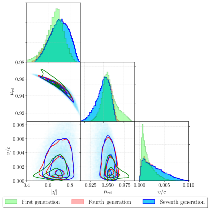
Kick velocity is also an output of the surrogate code. It is, therefore, reasonable to evaluate the fixed-point convergence of the three-dimensional joint distribution $p(\mu_{\mathrm{rel}},\chi,v/c)$ as plotted in Fig. 10. The panel showing the marginalized distribution $p(\mu_{\mathrm{rel}},\chi)$ shows the same convergence seen in Fig. 2, in addition to the panels $p(v/c,\chi)$ and $p(v/c,\mu_{\mathrm{rel}})$ which are also consistent with the convergence to a fixed-point distribution. This corner plot was produced using $N_{\mathrm{samp}}=40,000$ instead of the 2000 samples used throughout much of the paper. This change did not affect any of our results. The bottom row in this corner plot shows that the kick velocity distribution also converges to a fixed-point.

Figure 12: Central mass (left) and spin (right) moments, made dimensionless in units of mean mass and spin, as a function of generation. The mass moments all seem to decrease until the twelfth generation, where the moments become constant. The spin moments converge more quickly.

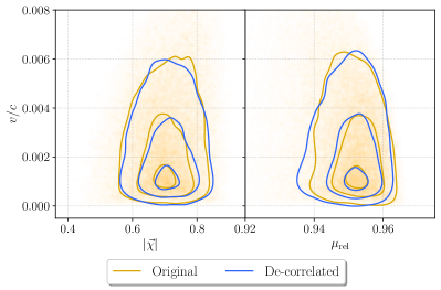
The marginalized distributions $p(v/c,\chi)$ and $p(v/c,\mu_{\mathrm{rel}})$ show low correlations between the kick velocity and either $\chi$ or $\mu_{\mathrm{rel}}$. To verify this, we created a de-correlated distribution by starting with the fixed-point distribution, and permuting the values of $v/c$ among the samples. This does not affect the marginalized distribution $p(v/c)$, while breaking any correlations between $v/c$ and all other variables. We show 30%, 68%, and 95% contours of the original and de-correlated distributions in Fig. 11. The two sets of contours are very similar, suggesting the remnant kick velocity is approximately independent of the remnant spin and relative mass ratio.

It is also possible to quantify the convergence of the three-dimensional joint distributions by computing the KL divergence, as indicated in Section III. We found a decrement in the magnitude of $D_{\mathrm{KL}}$ as the number of generations increases, which is similar to our results in Fig. 7 for the joint $(\mu_{\mathrm{rel}},\chi)$ distribution. The minimum value of $D_{\mathrm{KL}}$ grows with the number of dimensions of parameter space. Kernel density estimation is also noisier in higher dimensions, so the 3D results are noisier than the 2D results. Still, convergence to a fixed-point happens in the same number of generations.

Appendix B Evolution of moments of distributions

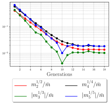
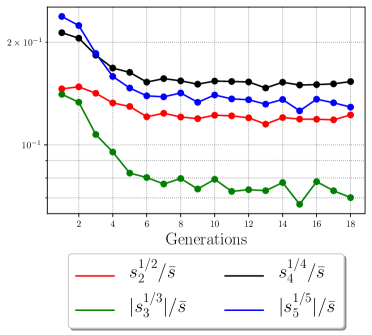
Another way to quantify the convergence of these distributions is to evaluate various central moments of the one-dimensional marginalized distributions. With the average mass as $\bar{m}=\langle m\rangle$, we define the $k$th central mass moment as $m_{k}\equiv\langle(m-\bar{m})^{k}\rangle$, and similarly for spin. These quantities moments carry dimensions of mass (or spin) to the power $k$, so they can be made dimensionless by computing $|m_{k}|^{1/k}/\bar{m}$ (and likewise for spin). We plot these dimensionless central moments in Fig. 12, as a function of generation, using the Kroupa power law as the initial condition on mass.

In the left panel, note that all of the moments decrease until a large number of generations. In particular, the ratio of the variance with the mean mass, $m_{2}/\bar{m}$, is consistent with narrowing of the marginal mass distribution visible in Figs. 3 and 6. After twelve generations of mergers, the shape of the mass distribution is approximately constant. The number of generations needed to observe the approximate invariance of the mass distribution shape reduces if we choose (log-)normal or thermal initial conditions. The scaled central moments of the marginal spin distribution appear in the right panel, and also converge after five generation, as seen previously. In both panels, skewness ($m_{3}$ and $s_{3}$) is not dominant, though, not all odd moments are negligible. Thus, even when the fixed-point distribution is centrally-peaked, it is not a Gaussian.

References

- Bekenstein (1973) Jacob D. Bekenstein, “Black holes and entropy,” Phys. Rev. D 7, 2333–2346 (1973).
- Bekenstein (1974) Jacob D. Bekenstein, “Generalized second law of thermodynamics in black hole physics,” Phys. Rev. D 9, 3292–3300 (1974).
- Bekenstein (1975) J.D. Bekenstein, “Statistical Black Hole Thermodynamics,” Phys. Rev. D 12, 3077–3085 (1975).
- Hawking (1975) S. W. Hawking, “Particle Creation by Black Holes,” Euclidean quantum gravity, Commun. Math. Phys. 43, 199–220 (1975), [Erratum: Commun. Math. Phys.46,206(1976)].
- Strominger and Vafa (1996) Andrew Strominger and Cumrun Vafa, “Microscopic origin of the Bekenstein-Hawking entropy,” Phys. Lett. B379, 99–104 (1996), arXiv:hep-th/9601029 [hep-th] .
- Ashtekar et al. (1998) A. Ashtekar, J. Baez, A. Corichi, and Kirill Krasnov, “Quantum geometry and black hole entropy,” Phys. Rev. Lett. 80, 904–907 (1998), arXiv:gr-qc/9710007 [gr-qc] .
- Fryer and Kalogera (2001) Chris L. Fryer and Vassiliki Kalogera, “Theoretical black hole mass distributions,” Astrophys. J. 554, 548–560 (2001), arXiv:astro-ph/9911312 [astro-ph] .
- Berti and Volonteri (2008) Emanuele Berti and Marta Volonteri, “Cosmological black hole spin evolution by mergers and accretion,” Astrophys. J. 684, 822–828 (2008), arXiv:0802.0025 [astro-ph] .
- Gerosa et al. (2018) Davide Gerosa, Emanuele Berti, Richard O’Shaughnessy, Krzysztof Belczynski, Michael Kesden, Daniel Wysocki, and Wojciech Gladysz, “Spin orientations of merging black holes formed from the evolution of stellar binaries,” Phys. Rev. D98, 084036 (2018), arXiv:1808.02491 [astro-ph.HE] .
- Kimball et al. (2019) Chase Kimball, Christopher P.L. Berry, and Vicky Kalogera, “What GW170729’s exceptional mass and spin tells us about its family tree,” (2019), 10.3847/2515-5172/ab66be, arXiv:1903.07813 [astro-ph.HE] .
- Kimball et al. (2020) Chase Kimball, Colm Talbot, Christopher P. L. Berry, Matthew Carney, Michael Zevin, Eric Thrane, and Vicky Kalogera, “Black hole genealogy: Identifying hierarchical mergers with gravitational waves,” (2020), arXiv:2005.00023 [astro-ph.HE] .
- Gerosa and Berti (2019) Davide Gerosa and Emanuele Berti, “Escape speed of stellar clusters from multiple-generation black-hole mergers in the upper mass gap,” Phys. Rev. D 100, 041301 (2019), arXiv:1906.05295 [astro-ph.HE] .
- Rodriguez et al. (2019) Carl L. Rodriguez, Michael Zevin, Pau Amaro-Seoane, Sourav Chatterjee, Kyle Kremer, Frederic A. Rasio, and Claire S. Ye, “Black holes: The next generation—repeated mergers in dense star clusters and their gravitational-wave properties,” Phys. Rev. D 100, 043027 (2019), arXiv:1906.10260 [astro-ph.HE] .
- Banerjee (2020) Sambaran Banerjee, “Stellar-mass black holes in young massive and open stellar clusters IV: updated stellar-evolutionary and black hole spin models and comparisons with the LIGO-Virgo O1/O2 merger-event data,” (2020), arXiv:2004.07382 [astro-ph.HE] .
- Carr and Kuhnel (2020) Bernard Carr and Florian Kuhnel, “Primordial Black Holes as Dark Matter: Recent Developments,” Annual Review of Nuclear and Particle Science 70, 355–394 (2020), arXiv:2006.02838 [astro-ph.CO] .
- Raccanelli et al. (2018) Alvise Raccanelli, Francesca Vidotto, and Licia Verde, “Effects of primordial black holes quantum gravity decay on galaxy clustering,” JCAP 08, 003 (2018), arXiv:1708.02588 [astro-ph.CO] .
- Bianchi et al. (2018) Eugenio Bianchi, Anuradha Gupta, Hal M. Haggard, and B.S. Sathyaprakash, “Quantum gravity and black hole spin in gravitational wave observations: a test of the Bekenstein-Hawking entropy,” (2018), arXiv:1812.05127 [gr-qc] .
- Abbott et al. (2016) B.P. Abbott et al. (LIGO Scientific, Virgo), “Observation of Gravitational Waves from a Binary Black Hole Merger,” Phys. Rev. Lett. 116, 061102 (2016), arXiv:1602.03837 [gr-qc] .
- Abbott et al. (2017a) Benjamin P. Abbott et al. (LIGO Scientific, VIRGO), “GW170104: Observation of a 50-Solar-Mass Binary Black Hole Coalescence at Redshift 0.2,” Phys. Rev. Lett. 118, 221101 (2017a), [Erratum: Phys.Rev.Lett. 121, 129901 (2018)], arXiv:1706.01812 [gr-qc] .
- Abbott et al. (2017b) B.P. Abbott et al. (LIGO Scientific, Virgo), “GW170817: Observation of Gravitational Waves from a Binary Neutron Star Inspiral,” Phys. Rev. Lett. 119, 161101 (2017b), arXiv:1710.05832 [gr-qc] .
- Abbott et al. (2019a) B.P. Abbott et al. (LIGO Scientific, Virgo), “GWTC-1: A Gravitational-Wave Transient Catalog of Compact Binary Mergers Observed by LIGO and Virgo during the First and Second Observing Runs,” Phys. Rev. X 9, 031040 (2019a), arXiv:1811.12907 [astro-ph.HE] .
- Abbott et al. (2019b) B.P. Abbott et al. (LIGO Scientific, Virgo), “Binary Black Hole Population Properties Inferred from the First and Second Observing Runs of Advanced LIGO and Advanced Virgo,” Astrophys. J. Lett. 882, L24 (2019b), arXiv:1811.12940 [astro-ph.HE] .
- Abbott et al. (2020) R. Abbott et al. (LIGO Scientific, Virgo), “GW190412: Observation of a Binary-Black-Hole Coalescence with Asymmetric Masses,” (2020), arXiv:2004.08342 [astro-ph.HE] .
- Boyle et al. (2019) Michael Boyle et al., “The SXS Collaboration catalog of binary black hole simulations,” Class. Quant. Grav. 36, 195006 (2019), arXiv:1904.04831 [gr-qc] .
- Varma et al. (2019a) Vijay Varma, Davide Gerosa, Leo C. Stein, Francois Hébert, and Hao Zhang, “High-accuracy mass, spin, and recoil predictions of generic black-hole merger remnants,” Phys. Rev. Lett. 122, 011101 (2019a), arXiv:1809.09125 [gr-qc] .
- Varma et al. (2019b) Vijay Varma, Scott E. Field, Mark A. Scheel, Jonathan Blackman, Davide Gerosa, Leo C. Stein, Lawrence E. Kidder, and Harald P. Pfeiffer, “Surrogate models for precessing binary black hole simulations with unequal masses,” Phys. Rev. Research. 1, 033015 (2019b), arXiv:1905.09300 [gr-qc] .
- Tichy and Marronetti (2008) Wolfgang Tichy and Pedro Marronetti, “The Final mass and spin of black hole mergers,” Phys. Rev. D 78, 081501 (2008), arXiv:0807.2985 [gr-qc] .
- Barausse et al. (2012) Enrico Barausse, Viktoriya Morozova, and Luciano Rezzolla, “On the mass radiated by coalescing black-hole binaries,” Astrophys. J. 758, 63 (2012), [Erratum: Astrophys.J. 786, 76 (2014)], arXiv:1206.3803 [gr-qc] .
- Hofmann et al. (2016) Fabian Hofmann, Enrico Barausse, and Luciano Rezzolla, “The final spin from binary black holes in quasi-circular orbits,” Astrophys. J. Lett. 825, L19 (2016), arXiv:1605.01938 [gr-qc] .
- Gerosa and Kesden (2016) Davide Gerosa and Michael Kesden, “PRECESSION: Dynamics of spinning black-hole binaries with python,” Phys. Rev. D 93, 124066 (2016), arXiv:1605.01067 [astro-ph.HE] .
- Campanelli et al. (2007) Manuela Campanelli, Carlos O. Lousto, Yosef Zlochower, and David Merritt, “Large merger recoils and spin flips from generic black-hole binaries,” Astrophys. J. Lett. 659, L5–L8 (2007), arXiv:gr-qc/0701164 .
- Gonzalez et al. (2007) Jose A. Gonzalez, Ulrich Sperhake, Bernd Bruegmann, Mark Hannam, and Sascha Husa, “Total recoil: The Maximum kick from nonspinning black-hole binary inspiral,” Phys. Rev. Lett. 98, 091101 (2007), arXiv:gr-qc/0610154 .
- Lousto and Zlochower (2008) Carlos O. Lousto and Yosef Zlochower, “Further insight into gravitational recoil,” Phys. Rev. D 77, 044028 (2008), arXiv:0708.4048 [gr-qc] .
- Lousto et al. (2012) Carlos O. Lousto, Yosef Zlochower, Massimo Dotti, and Marta Volonteri, “Gravitational Recoil From Accretion-Aligned Black-Hole Binaries,” Phys. Rev. D 85, 084015 (2012), arXiv:1201.1923 [gr-qc] .
- Lousto and Zlochower (2013) Carlos O. Lousto and Yosef Zlochower, “Nonlinear Gravitational Recoil from the Mergers of Precessing Black-Hole Binaries,” Phys. Rev. D 87, 084027 (2013), arXiv:1211.7099 [gr-qc] .
- Kullback and Leibler (1951) S. Kullback and R. A. Leibler, “On information and sufficiency,” Ann. Math. Statist. 22, 79–86 (1951).
- Hughes and Blandford (2003) Scott A. Hughes and Roger D. Blandford, “Black hole mass and spin coevolution by mergers,” Astrophys. J. Lett. 585, L101–L104 (2003), arXiv:astro-ph/0208484 .
- Rifat et al. (2020) Nur E. M. Rifat, Scott E. Field, Gaurav Khanna, and Vijay Varma, “Surrogate model for gravitational wave signals from comparable and large-mass-ratio black hole binaries,” Phys. Rev. D101, 081502 (2020), arXiv:1910.10473 [gr-qc] .
- Babak et al. (2017) Stanislav Babak, Andrea Taracchini, and Alessandra Buonanno, “Validating the effective-one-body model of spinning, precessing binary black holes against numerical relativity,” Phys. Rev. D95, 024010 (2017), arXiv:1607.05661 [gr-qc] .
- Fishbach and Holz (2020) Maya Fishbach and Daniel E. Holz, “Picky Partners: The Pairing of Component Masses in Binary Black Hole Mergers,” Astrophys. J. Lett. 891, L27 (2020), arXiv:1905.12669 [astro-ph.HE] .
- Kroupa (2001) Pavel Kroupa, “On the variation of the initial mass function,” Mon. Not. Roy. Astron. Soc. 322, 231 (2001), arXiv:astro-ph/0009005 .
- Gerosa and Berti (2017) Davide Gerosa and Emanuele Berti, “Are merging black holes born from stellar collapse or previous mergers?” Phys. Rev. D 95, 124046 (2017), arXiv:1703.06223 [gr-qc] .
- Gerosa et al. (2020) Davide Gerosa, Salvatore Vitale, and Emanuele Berti, “Astrophysical implications of GW190412 as a remnant of a previous black-hole merger,” (2020), arXiv:2005.04243 [astro-ph.HE] .
- Fishbach et al. (2017) Maya Fishbach, Daniel E. Holz, and Ben Farr, “Are LIGO’s Black Holes Made From Smaller Black Holes?” Astrophys. J. Lett. 840, L24 (2017), arXiv:1703.06869 [astro-ph.HE] .
- Pretorius (2005) Frans Pretorius, “Evolution of binary black hole spacetimes,” Phys. Rev. Lett. 95, 121101 (2005), arXiv:gr-qc/0507014 [gr-qc] .
- Virtanen et al. (2020) Pauli Virtanen, Ralf Gommers, Travis E. Oliphant, Matt Haberland, Tyler Reddy, David Cournapeau, Evgeni Burovski, Pearu Peterson, Warren Weckesser, Jonathan Bright, Stéfan J. van der Walt, Matthew Brett, Joshua Wilson, K. Jarrod Millman, Nikolay Mayorov, Andrew R. J. Nelson, Eric Jones, Robert Kern, Eric Larson, CJ Carey, İlhan Polat, Yu Feng, Eric W. Moore, Jake Vand erPlas, Denis Laxalde, Josef Perktold, Robert Cimrman, Ian Henriksen, E. A. Quintero, Charles R Harris, Anne M. Archibald, Antônio H. Ribeiro, Fabian Pedregosa, Paul van Mulbregt, and SciPy 1. 0 Contributors, “SciPy 1.0: Fundamental Algorithms for Scientific Computing in Python,” Nature Methods 17, 261–272 (2020).
- Carroll and Chen (2004) Sean M. Carroll and Jennifer Chen, “Spontaneous inflation and the origin of the arrow of time,” (2004), arXiv:hep-th/0410270 .
- Egan and Lineweaver (2010) Chas A. Egan and Charles H. Lineweaver, “A Larger Estimate of the Entropy of the Universe,” Astrophys. J. 710, 1825–1834 (2010), arXiv:0909.3983 [astro-ph.CO] .
- Rodriguez-Gomez et al. (2015) Vicente Rodriguez-Gomez et al., “The merger rate of galaxies in the Illustris Simulation: a comparison with observations and semi-empirical models,” Mon. Not. Roy. Astron. Soc. 449, 49–64 (2015), arXiv:1502.01339 [astro-ph.GA] .
- Arzoumanian et al. (2018) Z. Arzoumanian et al. (NANOGRAV), “The NANOGrav 11-year Data Set: Pulsar-timing Constraints On The Stochastic Gravitational-wave Background,” Astrophys. J. 859, 47 (2018), arXiv:1801.02617 [astro-ph.HE] .
- Chen et al. (2019) Siyuan Chen, Alberto Sesana, and Christopher J. Conselice, “Constraining astrophysical observables of Galaxy and Supermassive Black Hole Binary Mergers using Pulsar Timing Arrays,” Mon. Not. Roy. Astron. Soc. 488, 401–418 (2019), arXiv:1810.04184 [astro-ph.GA] .
- Reali et al. (2020) Luca Reali, Matthew Mould, Davide Gerosa, and Vijay Varma, “Mapping the asymptotic inspiral of precessing binary black holes to their merger remnants,” (2020), arXiv:2005.01747 [gr-qc] .
- Christian et al. (2018) Pierre Christian, Philip Mocz, and Abraham Loeb, “Evolution of the Black Hole Mass Function in Star Clusters from Multiple Mergers,” Astrophys. J. Lett. 858, L8 (2018), arXiv:1803.07094 [astro-ph.HE] .
- Harris et al. (2020) Charles R. Harris, K. Jarrod Millman, Stéfan J van der Walt, Ralf Gommers, Pauli Virtanen, David Cournapeau, Eric Wieser, Julian Taylor, Sebastian Berg, Nathaniel J. Smith, Robert Kern, Matti Picus, Stephan Hoyer, Marten H. van Kerkwijk, Matthew Brett, Allan Haldane, Jaime Fernández del Río, Mark Wiebe, Pearu Peterson, Pierre Gérard-Marchant, Kevin Sheppard, Tyler Reddy, Warren Weckesser, Hameer Abbasi, Christoph Gohlke, and Travis E. Oliphant, “Array programming with NumPy,” Nature 585, 357–362 (2020).