Autonomous Tracking and State Estimation with Generalised Group Lasso

Rui Gao, Simo Särkkä, Rubén Claveria-Vega, and Simon Godsill R. Gao and S. Särkkä are with the Department of Electrical Engineering and Automation, Aalto University, Espoo, 02150 Finland (e-mail:rui.gao@aalto.fi; simo.sarkka@aalto.fi). R. Claveria-Vega and S. Godsill are with the Department of Engineering, University of Cambridge, CB2 1PZ, UK (e-mail:rmc83@cam.ac.uk; sjg@eng.cam.ac.uk). This work was supported by Academy of Finland.
Abstract

We address the problem of autonomous tracking and state estimation for marine vessels, autonomous vehicles, and other dynamic signals under a (structured) sparsity assumption. The aim is to improve the tracking and estimation accuracy with respect to classical Bayesian filters and smoothers. We formulate the estimation problem as a dynamic generalised group Lasso problem and develop a class of smoothing-and-splitting methods to solve it. The Levenberg–Marquardt iterated extended Kalman smoother-based multi-block alternating direction method of multipliers (LM-IEKS-mADMM) algorithms are based on the alternating direction method of multipliers (ADMM) framework. This leads to minimisation subproblems with an inherent structure to which three new augmented recursive smoothers are applied. Our methods can deal with large-scale problems without pre-processing for dimensionality reduction. Moreover, the methods allow one to solve nonsmooth nonconvex optimisation problems. We then prove that under mild conditions, the proposed methods converge to a stationary point of the optimisation problem. By simulated and real-data experiments including multi-sensor range measurement problems, marine vessel tracking, autonomous vehicle tracking, and audio signal restoration, we show the practical effectiveness of the proposed methods.

Index Terms:
Autonomous tracking, state estimation, Kalman smoother, alternating direction method of multipliers (ADMM), sparsity, group Lasso.

I Introduction

Autonomous tracking and state estimation problems are active research topics with many real-world applications, including intelligent maritime navigation, autonomous vehicle tracking, and audio signal estimation [1, 2, 3, 4, 5]. The aim is to autonomously estimate and track the state (e.g., position, velocity, or direction) of the dynamic system using imperfect measurements [6]. A frequently used approach for autonomous tracking and estimation problems is based on Bayesian filtering and smoothing. When the target dynamics and observation models are linear and Gaussian, Kalman smoother (KS) [1, 7] provides the optimal Bayesian solution which coincides with the optimal minimum mean square error estimator in that case. In the case of nonlinear dynamic systems, the iterated extended Kalman smoother (IEKS) [8, 9, 10] makes use of local affine approximations by means of Taylor series for the nonlinear functions, and then iteratively carries out KS. Sigma-point based smoothing methods [11, 12] employ sigma-points to approximate the probability density of the states, which can preserve higher-order accuracy than IEKS. Random sampling-based filters such as particle filters [13, 14, 1, 15] can be used to deal with nonlinear tracking situations involving potentially arbitrary nonlinearities, noise, and constraints. Although these trackers and estimators are capable of utilising the measurement information to obtain the estimates, they ignore sparsity dictated by physical attributes of dynamic systems.

The motivation for our work comes from the following real-world applications. One significant application is marine vessel tracking [5, 6]. Vessels are frequently pitching and rolling on the surface of the ocean, which can be modelled as sparsity in the process noise. Our methodology is also applicable to autonomous vehicle tracking, which enables a vehicle to autonomously avoid obstacles and maintain safe distances to other vehicles. In presence of many sudden stops (i.e., velocities are zero), the tracking accuracy can be improved by employing sparsity [16]. Other examples of tracked targets include robots [9] and unmanned aerial vehicles [17]. Another practical application is audio signal restoration, where typically only a few time-frequency elements are expected to be present, and thus, sparsity is an advisable assumption [18]. For example, Gabor synthesis representation with sparsity constraints has been proved to be suitable for audio restoration [19]. Similar problems can also be found in electrocardiogram (ECG) signal analysis [20] and automatic music transcription [21]. Hence, computationally effective sparsity modelling methods are in demand.

Since sparsity may improve the tracking and estimation performance, there is a growing literature that proposes sparse regularisers such as Lasso (i.e., least absolute shrinkage and selection operator, or L1subscript𝐿1L_{1}-regularisation) [22, 23] or total variation (TV) [24, 25] for these applications. Existing methods for sparse tracking and estimation can be split in two broad categories: robust smoothing approaches and optimisation-based approaches. The former approaches merge filtering and smoothing with L1subscript𝐿1L_{1}-regularisation. For instance, the modified recursive filter-based compressive sensing methods were developed in [26, 27, 28, 29]. An L1subscript𝐿1L_{1}-Laplace robust Kalman smoother was presented in [30]. Using both sparsity and dynamics information, a sparse Bayesian learning framework was proposed in [31]. The latter approaches formulate the whole tracking and state estimation problem as an L1subscript𝐿1L_{1}-penalised minimisation problem, and then apply iterative algorithms to solve the minimisation problem [32, 33, 16, 34, 35, 36]. While these L1subscript𝐿1L_{1}-penalised estimators offer several benefits, they penalise individual elements of the state vector or process noise instead of groups of elements in them.

Recently, there have been important advances in the structured sparsity methodology for collision avoidance [37, 38], path-following and tracking [39, 40], and visual tracking [41, 42]. In [43], a discriminative supervised hashing method was proposed for object tracking tasks. An adaptive elastic echo state network was developed for multivariate time series prediction in [44]. The work in [45] formulated a moving tracking problem with L2subscript𝐿2L_{2}-norm constraints and then introduced a temporal consistency dictionary learning algorithm. However, the methods lack strong convergence and performance guarantees, particularly when the objective becomes nonconvex. Moreover, relatively few methods exist for incorporating structured sparsity into autonomous tracking and state estimation problems. Taking these developments into consideration, the main goal here is to develop new efficient methods for regularised autonomous tracking and estimation problems, which allow for group Lasso type of sparseness assumptions on groups of state or process noise elements.

When we formulate a regularised autonomous tracking and state estimation problem as a generalised L2subscript𝐿2L_{2}-minimisation problem (also called as dynamic generalised group Lasso problem), the resulting problem is difficult to solve due to its nonsmoothness and/or nonconvexity. Splitting-based optimisation methods [46, 47, 48] such as multi-block alternating direction method of multipliers (ADMM) [47], are methods that can tackle this kind of problems. One advantage of these methods is that they decompose the original problem into a sequence of easier subproblems. Although these methods can directly work on the original optimisation problem, such direct use ignores the inherent structure induced by the implied Markovian structure in the optimisation problem. In this paper, we propose a class of efficient smoothing-and-splitting methods that outperform the classical optimisation methods in terms of computational time due to the leveraging of the Markovian structure.

In this paper, we focus on autonomous tracking and state estimation problems with sparsity-inducing priors. Our first contribution is to provide a flexible formulation of dynamic generalised group Lasso problems arising in autonomous tracking and state estimation. Special cases of the formulation are Lasso, isotropic TV, anisotropic TV, fused Lasso, group Lasso, and sparse group Lasso. Meanwhile, the formulation can cope with sparsity on the process noise or the state in dynamic systems. Since the resulting optimisation problems are nonsmooth, possibly nonconvex, and large-dimensional, our second contribution is to provide a class of the smoothing-and-splitting methods to address them. We develop the new KS-mADMM, Gauss–Newton IEKS-mADMM (GN-IEKS-mADMM), and Levenberg–Marquardt IEKS-mADMM (LM-IEKS-mADMM) methods which use augmented recursive smoothers to solve the primal subproblems in the mADMM iterations. As a third contribution, we prove that under mild conditions, the proposed methods converge to a stationary point. Our fourth contribution is to apply the proposed methods to real-world applications of marine vessel tracking, autonomous vehicle tracking, and audio signal restoration.

The rest of this paper is structured as follows. In Section II, we formulate the sparse autonomous tracking and state estimation problem as a generalised L2subscript𝐿2L_{2}-minimisation problem. Particularly, we present a broad class of regulariser configurations parametrised by sets of matrices and vectors. We introduce the batch tracking and estimation methods in Section III and present three augmented recursive smoothing methods in Section IV. In Section V, we establish the convergence. In Section VI, we report numerical results on simulated and real-life datasets. Section VII draws the concluding remarks.

The notation is as follows. Matrices 𝐗𝐗\mathbf{X} and vectors 𝐱𝐱\mathbf{x} are indicated in boldface. ()superscripttop(\cdot)^{\top} represents transposition, and ()1superscript1(\cdot)^{-1} represents matrix inversion. The 𝐑𝐑\mathbf{R}-weighted norm of 𝐱𝐱\mathbf{x} is denoted by 𝐱𝐑=𝐱𝐑𝐱subscriptnorm𝐱𝐑superscript𝐱top𝐑𝐱\|\mathbf{x}\|_{\mathbf{R}}=\sqrt{\mathbf{x}^{\top}\mathbf{R}\mathbf{x}}. 𝐱1=|xi|subscriptnorm𝐱1subscript𝑥𝑖\left\|\mathbf{x}\right\|_{1}=\sum|x_{i}| denotes L1subscript𝐿1L_{1}-norm, and 𝐱2=ixi2subscriptnorm𝐱2subscript𝑖superscriptsubscript𝑥𝑖2\left\|\mathbf{x}\right\|_{2}=\sqrt{\sum_{i}x_{i}^{2}} denotes L2subscript𝐿2L_{2}-norm. 𝐗g,tsubscript𝐗𝑔𝑡\mathbf{X}_{g,t} is the (g,t)𝑔𝑡(g,t):th element of matrix 𝐗𝐗\mathbf{X}, and 𝐱(k)superscript𝐱𝑘\mathbf{x}^{(k)} denotes the value of 𝐱𝐱\mathbf{x} at k𝑘k:th iteration. vec()vec\operatorname{vec}(\cdot) represents a vectorisation operator, diag()diag\operatorname{diag}(\cdot) represents a block diagonal matrix operator with the elements in its argument on the diagonal, and 𝐱1:T=vec(𝐱1,,𝐱T)subscript𝐱:1𝑇vecsubscript𝐱1subscript𝐱𝑇\mathbf{x}_{1:T}=\operatorname{vec}(\mathbf{x}_{1},\ldots,\mathbf{x}_{T}). ϕ(𝐱)italic-ϕ𝐱\partial\phi(\mathbf{x}) denotes a sub-gradient of ϕitalic-ϕ\phi. 𝐉ϕsubscript𝐉italic-ϕ\mathbf{J}_{\phi} is the Jacobian of ϕ(𝐱)italic-ϕ𝐱{\phi}(\mathbf{x}). δ+(𝐀)subscript𝛿𝐀\delta_{+}(\mathbf{A}) denotes the smallest eigenvalue of 𝐀𝐀\mathbf{A}. p(𝐱)𝑝𝐱p(\mathbf{x}) denotes probability density function (pdf) of 𝐱𝐱\mathbf{x} and 𝒩(𝐱𝐦,𝐏)𝒩conditional𝐱𝐦𝐏\mathcal{N}(\mathbf{x}\mid\mathbf{m},\mathbf{P}) denotes a Gaussian probability density function with mean 𝐦𝐦\mathbf{m} and covariance 𝐏𝐏\mathbf{P} evaluated at 𝐱𝐱\mathbf{x}.

II Problem Statement

Let 𝐲tNysubscript𝐲𝑡superscriptsubscript𝑁𝑦\mathbf{y}_{t}\in\mathbb{R}^{N_{y}} be a measurement of a dynamic system and 𝐱tNxsubscript𝐱𝑡superscriptsubscript𝑁𝑥\mathbf{x}_{t}\in\mathbb{R}^{N_{x}} be an unknown state (sometimes called the source or signal). The state and measurement are related according to a dynamic state-space model of the form

𝐱t=𝐚t(𝐱t1)+𝐪t,𝐲t=𝐡t(𝐱t)+𝐫t,\begin{split}\mathbf{x}_{t}=\mathbf{a}_{t}(\mathbf{x}_{t-1})+\mathbf{q}_{t},\quad\mathbf{y}_{t}=\mathbf{h}_{t}(\mathbf{x}_{t})+\mathbf{r}_{t},\end{split} (1)

where 𝐡t:NxNy:subscript𝐡𝑡superscriptsubscript𝑁𝑥superscriptsubscript𝑁𝑦\mathbf{h}_{t}:\mathbb{R}^{N_{x}}\to\mathbb{R}^{N_{y}} and 𝐚t:NxNx:subscript𝐚𝑡superscriptsubscript𝑁𝑥superscriptsubscript𝑁𝑥\mathbf{a}_{t}:\mathbb{R}^{N_{x}}\to\mathbb{R}^{N_{x}} are the measurement and state transition functions, respectively, and t=1,,T𝑡1𝑇t=1,\ldots,T is the time step number. The process and measurement noises 𝐪t𝒩(𝟎,𝐐t)similar-tosubscript𝐪𝑡𝒩0subscript𝐐𝑡\mathbf{q}_{t}\sim\mathcal{N}(\mathbf{0},\mathbf{Q}_{t}) and 𝐫t𝒩(𝟎,𝐑t)similar-tosubscript𝐫𝑡𝒩0subscript𝐑𝑡\mathbf{r}_{t}\sim\mathcal{N}(\mathbf{0},\mathbf{R}_{t}) are assumed to be zero-mean Gaussian with covariances 𝐐tsubscript𝐐𝑡\mathbf{Q}_{t} and 𝐑tsubscript𝐑𝑡\mathbf{R}_{t}, respectively. The initial condition at t=1𝑡1t=1 is given by 𝐱1𝒩(𝐦1,𝐏1)similar-tosubscript𝐱1𝒩subscript𝐦1subscript𝐏1\mathbf{x}_{1}\sim\mathcal{N}(\mathbf{m}_{1},\mathbf{P}_{1}). A particular special case of (1) is an affine Gaussian model by

𝐚t(𝐱t1)=𝐀t𝐱t1+𝐛t,𝐡t(𝐱t)=𝐇t𝐱t+𝐞t,formulae-sequencesubscript𝐚𝑡subscript𝐱𝑡1subscript𝐀𝑡subscript𝐱𝑡1subscript𝐛𝑡subscript𝐡𝑡subscript𝐱𝑡subscript𝐇𝑡subscript𝐱𝑡subscript𝐞𝑡\displaystyle\mathbf{a}_{t}(\mathbf{x}_{t-1})=\mathbf{A}_{t}\,\mathbf{x}_{t-1}+\mathbf{b}_{t},\quad\mathbf{h}_{t}(\mathbf{x}_{t})=\mathbf{H}_{t}\,\mathbf{x}_{t}+\mathbf{e}_{t}, (2)

where 𝐀tNx×Nxsubscript𝐀𝑡superscriptsubscript𝑁𝑥subscript𝑁𝑥\mathbf{A}_{t}\in\mathbb{R}^{N_{x}\times N_{x}}, 𝐇tNy×Nxsubscript𝐇𝑡superscriptsubscript𝑁𝑦subscript𝑁𝑥\mathbf{H}_{t}\in\mathbb{R}^{N_{y}\times N_{x}} are the transition and measurement matrices, and 𝐛tsubscript𝐛𝑡\mathbf{b}_{t}, 𝐞tsubscript𝐞𝑡\mathbf{e}_{t} are bias terms.

The goal here is to obtain the “best estimate” of 𝐱1:Tsubscript𝐱:1𝑇\mathbf{x}_{1:T} from imperfect measurements 𝐲1:Tsubscript𝐲:1𝑇\mathbf{y}_{1:T}. For computing 𝐱1:Tsubscript𝐱:1𝑇\mathbf{x}_{1:T} with sparsity-inducing priors, we define a set of matrices {𝐆g,tPg×Nxg=1,,Ng}conditional-setsubscript𝐆𝑔𝑡superscriptsubscript𝑃𝑔subscript𝑁𝑥𝑔1subscript𝑁𝑔\left\{\mathbf{G}_{g,t}\in\mathbb{R}^{P_{g}\times N_{x}}\mid g=1,\ldots,N_{g}\right\}, matrices 𝐁tsubscript𝐁𝑡\mathbf{B}_{t}, and vectors 𝐝tsubscript𝐝𝑡\mathbf{d}_{t}, for t=1,,T𝑡1𝑇t=1,\ldots,T, and impose sparsity on the groups of elements of the state or the process noise. Mathematically, the problem of computing the state estimate 𝐱1:Tsubscriptsuperscript𝐱:1𝑇\mathbf{x}^{\star}_{1:{T}} is formulated as

𝐱1:T=argmin𝐱1:T12t=1T𝐲t𝐡t(𝐱t)𝐑t12+12t=2T𝐱t𝐚t(𝐱t1)𝐐t12+12𝐱1𝐦1𝐏112+t=1Tg=1Ngμ𝐆g,t(𝐱t𝐁t𝐱t1𝐝t)2,missing-subexpressionsubscriptsuperscript𝐱:1𝑇subscriptsubscript𝐱:1𝑇12superscriptsubscript𝑡1𝑇superscriptsubscriptnormsubscript𝐲𝑡subscript𝐡𝑡subscript𝐱𝑡superscriptsubscript𝐑𝑡12missing-subexpression12superscriptsubscript𝑡2𝑇superscriptsubscriptnormsubscript𝐱𝑡subscript𝐚𝑡subscript𝐱𝑡1superscriptsubscript𝐐𝑡1212superscriptsubscriptnormsubscript𝐱1subscript𝐦1superscriptsubscript𝐏112missing-subexpressionsuperscriptsubscript𝑡1𝑇superscriptsubscript𝑔1subscript𝑁𝑔𝜇subscriptnormsubscript𝐆𝑔𝑡subscript𝐱𝑡subscript𝐁𝑡subscript𝐱𝑡1subscript𝐝𝑡2\begin{split}\begin{aligned} &\mathbf{x}^{\star}_{1:{T}}=\arg\min_{\mathbf{x}_{1:{T}}}\frac{1}{2}\sum_{t=1}^{T}\left\|\mathbf{y}_{t}-\mathbf{h}_{t}(\mathbf{x}_{t})\right\|_{\mathbf{R}_{t}^{-1}}^{2}\\ &\quad+\frac{1}{2}\sum_{t=2}^{T}\left\|\mathbf{x}_{t}-\mathbf{a}_{t}(\mathbf{x}_{t-1})\right\|_{\mathbf{Q}_{t}^{-1}}^{2}+\frac{1}{2}\left\|\mathbf{x}_{1}-\mathbf{m}_{1}\right\|_{\mathbf{P}_{1}^{-1}}^{2}\\ &\qquad+\sum_{t=1}^{T}\sum_{g=1}^{N_{g}}\mu\left\|\mathbf{G}_{g,t}\left(\mathbf{x}_{t}-\mathbf{B}_{t}\,\mathbf{x}_{t-1}-\mathbf{d}_{t}\right)\right\|_{2},\\ \end{aligned}\end{split} (3)

where μ>0𝜇0\mu>0 is a penalty parameter.

A merit of our formulation is its flexibility, because the selections of 𝐆g,tsubscript𝐆𝑔𝑡\mathbf{G}_{g,t}, 𝐁tsubscript𝐁𝑡\mathbf{B}_{t}, and 𝐝tsubscript𝐝𝑡\mathbf{d}_{t} can be adjusted to represent different regularisers. With matrix 𝐆g,tsubscript𝐆𝑔𝑡\mathbf{G}_{g,t}, the formulation (3) accommodates a large class of sparsity-promoting regularisers (e.g., Lasso, isotopic TV, anisotopic TV, fused Lasso, group Lasso, and sparse group Lasso). A list of such regularisers is reported in Table I. Meanwhile, the formulation (3) also allows for putting sparsity assumptions on the state or the process noise by different selections of 𝐁tsubscript𝐁𝑡\mathbf{B}_{t} and 𝐝tsubscript𝐝𝑡\mathbf{d}_{t} (see Table II).

TABLE I: Examples of sparsity-promoting regularisers that are included in the present framework.
Regularisation 𝐆g,tsubscript𝐆𝑔𝑡\mathbf{G}_{g,t} descriptions
L2subscript𝐿2L_{2}-regularisation 𝐆g,tsubscript𝐆𝑔𝑡\mathbf{G}_{g,t} is an identity matrix
Lasso
Ng=Nxsubscript𝑁𝑔subscript𝑁𝑥N_{g}=N_{x}, Pg=1subscript𝑃𝑔1P_{g}=1 for all g𝑔g,
𝐆g,tsubscript𝐆𝑔𝑡\mathbf{G}_{g,t} has 111 at g𝑔g:th column and zeros otherwise.
Isotopic TV
Ng=1subscript𝑁𝑔1N_{g}=1, P1=Nx1subscript𝑃1subscript𝑁𝑥1P_{1}=N_{x}-1
𝐆1,tsubscript𝐆1𝑡\mathbf{G}_{1,t} encodes a finite difference operator.
Anisotopic TV
𝐆g,tsubscript𝐆𝑔𝑡\mathbf{G}_{g,t} encodes the g𝑔g:th row of
a finite difference operator.
Fused Lasso
g=1,,Nx𝑔1subscript𝑁𝑥g=1,\ldots,N_{x}, Pg=1subscript𝑃𝑔1P_{g}=1 for all g𝑔g,
𝐆g,tsubscript𝐆𝑔𝑡\mathbf{G}_{g,t} has 111 at g𝑔g:th column and zeros otherwise;
g=Nx+1,,Ng𝑔subscript𝑁𝑥1subscript𝑁𝑔g=N_{x}+1,\ldots,N_{g}, 𝐆g,tsubscript𝐆𝑔𝑡\mathbf{G}_{g,t} encodes the g𝑔g:th row of
a finite difference operator.
Group Lasso
𝐆g,tsubscript𝐆𝑔𝑡\mathbf{G}_{g,t} has 111, corresponding to the selected elements
of 𝐱tsubscript𝐱𝑡\mathbf{x}_{t} in the group and zeros otherwise.
Sparse group Lasso
g=1,,Nx𝑔1subscript𝑁𝑥g=1,\ldots,N_{x}, Pg=1subscript𝑃𝑔1P_{g}=1,
𝐆g,tsubscript𝐆𝑔𝑡\mathbf{G}_{g,t} has 111 at g𝑔g:th column and zeros otherwise;
g=Nx+1,,Ng𝑔subscript𝑁𝑥1subscript𝑁𝑔g=N_{x}+1,\ldots,N_{g},
𝐆g,tsubscript𝐆𝑔𝑡\mathbf{G}_{g,t} has the same setting with group Lasso.
TABLE II: Flexible sparsity assumptions by selecting 𝐁tsubscript𝐁𝑡\mathbf{B}_{t} and 𝐝tsubscript𝐝𝑡\mathbf{d}_{t}.
Dynamic systems Sparsity on: 𝐁tsubscript𝐁𝑡\mathbf{B}_{t} and 𝐝tsubscript𝐝𝑡\mathbf{d}_{t}
Affine Gaussian state Settings on 𝐁t=𝟎subscript𝐁𝑡0\mathbf{B}_{t}=\mathbf{0}, 𝐝t=𝟎subscript𝐝𝑡0\mathbf{d}_{t}=\mathbf{0}
process noise 𝐁t=𝐀tsubscript𝐁𝑡subscript𝐀𝑡\mathbf{B}_{t}=\mathbf{A}_{t}, 𝐝t=𝐛tsubscript𝐝𝑡subscript𝐛𝑡\mathbf{d}_{t}=\mathbf{b}_{t}
Nonlinear state 𝐁t=𝟎subscript𝐁𝑡0\mathbf{B}_{t}=\mathbf{0}, 𝐝t=𝟎subscript𝐝𝑡0\mathbf{d}_{t}=\mathbf{0}
process noise
𝐁t𝐱t1+𝐝tsubscript𝐁𝑡subscript𝐱𝑡1subscript𝐝𝑡\mathbf{B}_{t}\mathbf{x}_{t-1}\!+\!\mathbf{d}_{t} as the affine approximation
of 𝐚t(𝐱t1)subscript𝐚𝑡subscript𝐱𝑡1\mathbf{a}_{t}(\mathbf{x}_{t-1}) (see Section IV-B)

A simple, yet illustrative, example can be found in autonomous vehicle tracking. When there are stop-and-go points (e.g. vehicle stops) in the data, the zero-velocity and zero-angle values at those time points can be grouped together via the L2subscript𝐿2L_{2}-norm and 𝐆g,tsubscript𝐆𝑔𝑡\mathbf{G}_{g,t}. That means three elements can be forced to be equal to zero at the same time. Another application is in audio restoration, where the matrices 𝐆g,tsubscript𝐆𝑔𝑡\mathbf{G}_{g,t} are defined so that only two elements of the state 𝐱tsubscript𝐱𝑡\mathbf{x}_{t} – corresponding to the real and imaginary parts of a synthesis coefficient – are extracted at a time step. Thus, these pairs, which are associated with the same time-frequency basis functions, tend to be non-zero or zero together.

The problem (3) is more difficult to solve than the common L2subscript𝐿2L_{2}-minimisation problem (which corresponds to 𝐆g,t=𝐈subscript𝐆𝑔𝑡𝐈\mathbf{G}_{g,t}=\mathbf{I}, where 𝐈𝐈\mathbf{I} is an identity matrix) or the squared L2subscript𝐿2L_{2}-minimisation problem (the problem with 𝐆g,t()22superscriptsubscriptnormsubscript𝐆𝑔𝑡22\left\|\mathbf{G}_{g,t}(\cdot)\right\|_{2}^{2}), since the penalty term 𝐆g,t()2subscriptnormsubscript𝐆𝑔𝑡2\left\|\mathbf{G}_{g,t}(\cdot)\right\|_{2} is nonsmooth. Furthermore, 𝐆g,tsubscript𝐆𝑔𝑡\mathbf{G}_{g,t} is possibly rank-deficient matrix. In this paper, we first derive batch tracking and estimation methods, which are based on the batch computation of the state sequence. To speed up the batch methods, we then propose augmented recursive smoother methods for the primal variable update.

III Batch Tracking and Estimation Methods

In this section, we introduce the multi-block ADMM framework. Based on this framework, we derive batch algorithms for solving the regularised tracking and state estimation problem.

III-A The General Multi-block ADMM (mADMM) Framework

The methods that we develop are based on the multi-block ADMM [47]. The multi-block ADMM provides an algorithmic framework which is applicable to problems of the form (3), and it can be instantiated by defining the auxiliary variables and their update steps. We introduce auxiliary variables 𝐯tsubscript𝐯𝑡\mathbf{v}_{t} and 𝐰g,tsubscript𝐰𝑔𝑡\mathbf{w}_{g,t}, g=1,,Ng𝑔1subscript𝑁𝑔g=1,\ldots,N_{g}, t=1,,T𝑡1𝑇t=1,\ldots,T, and then build the following constraints

𝐱t𝐁t𝐱t1𝐝tsubscript𝐱𝑡subscript𝐁𝑡subscript𝐱𝑡1subscript𝐝𝑡\displaystyle\mathbf{x}_{t}-\mathbf{B}_{t}\,\mathbf{x}_{t-1}-\mathbf{d}_{t} =𝐯t,absentsubscript𝐯𝑡\displaystyle=\mathbf{v}_{t}, (4)
𝐰1,tsubscript𝐰1𝑡\displaystyle\mathbf{w}_{1,t} =𝐆1,t𝐯t,absentsubscript𝐆1𝑡subscript𝐯𝑡\displaystyle=\mathbf{G}_{1,t}\,\mathbf{v}_{t},
\displaystyle\,\,\,\vdots
𝐰Ng,tsubscript𝐰subscript𝑁𝑔𝑡\displaystyle\mathbf{w}_{N_{g},t} =𝐆Ng,t𝐯t.absentsubscript𝐆subscript𝑁𝑔𝑡subscript𝐯𝑡\displaystyle=\mathbf{G}_{N_{g},t}\,\mathbf{v}_{t}.

Note that in (4) we could alternatively introduce auxiliary variables 𝐰g,t=𝐆g,t(𝐱t𝐁t𝐱t1𝐝t)subscript𝐰𝑔𝑡subscript𝐆𝑔𝑡subscript𝐱𝑡subscript𝐁𝑡subscript𝐱𝑡1subscript𝐝𝑡{\mathbf{w}}_{g,t}=\mathbf{G}_{g,t}(\mathbf{x}_{t}-\mathbf{B}_{t}\,\mathbf{x}_{t-1}-\mathbf{d}_{t}), but this replacement would require 𝐆g,tsubscript𝐆𝑔𝑡\mathbf{G}_{g,t} to be invertible when using the augmented recursive smoothers later on. To avoid such restrictions, we employ variables 𝐯tsubscript𝐯𝑡\mathbf{v}_{t} and 𝐰g,tsubscript𝐰𝑔𝑡\mathbf{w}_{g,t} to build the more general constraints in this paper.

For simplicity of notation, we denote 𝐰t=[𝐰1,t,,𝐰Ng,t]subscript𝐰𝑡superscriptmatrixsuperscriptsubscript𝐰1𝑡topsuperscriptsubscript𝐰subscript𝑁𝑔𝑡toptop{\mathbf{w}}_{t}=\begin{bmatrix}\mathbf{w}_{1,t}^{\top},&\ldots,&\mathbf{w}_{N_{g},t}^{\top}\end{bmatrix}^{\top}, 𝐆t=[𝐆1,t,,𝐆Ng,t]subscript𝐆𝑡superscriptmatrixsuperscriptsubscript𝐆1𝑡topsuperscriptsubscript𝐆subscript𝑁𝑔𝑡toptop{\mathbf{G}}_{t}=\begin{bmatrix}\mathbf{G}_{1,t}^{\top},&\ldots,&\mathbf{G}_{N_{g},t}^{\top}\end{bmatrix}^{\top}, and then solve (3), using an equivalent constrained optimisation problem

min𝐱1:T,𝐰1:T,𝐯1:T12t=1T𝐲t𝐡t(𝐱t)𝐑t12+t=1Tg=1Ngμ𝐰g,t2+12t=2T𝐱t𝐚t(𝐱t1)𝐐t12+12𝐱1𝐦1𝐏112s.t.[𝐱t𝐁t𝐱t1𝐝t𝐰t]=[𝐈𝐆t]𝐯t,t=1,,T.missing-subexpressionsubscriptsubscript𝐱:1𝑇subscript𝐰:1𝑇subscript𝐯:1𝑇12superscriptsubscript𝑡1𝑇superscriptsubscriptnormsubscript𝐲𝑡subscript𝐡𝑡subscript𝐱𝑡superscriptsubscript𝐑𝑡12superscriptsubscript𝑡1𝑇superscriptsubscript𝑔1subscript𝑁𝑔𝜇subscriptnormsubscript𝐰𝑔𝑡2missing-subexpression12superscriptsubscript𝑡2𝑇superscriptsubscriptnormsubscript𝐱𝑡subscript𝐚𝑡subscript𝐱𝑡1superscriptsubscript𝐐𝑡1212superscriptsubscriptnormsubscript𝐱1subscript𝐦1superscriptsubscript𝐏112missing-subexpressionformulae-sequencestformulae-sequencematrixsubscript𝐱𝑡subscript𝐁𝑡subscript𝐱𝑡1subscript𝐝𝑡subscript𝐰𝑡matrix𝐈subscript𝐆𝑡subscript𝐯𝑡𝑡1𝑇\begin{split}\begin{aligned} &\min_{\begin{subarray}{c}\mathbf{x}_{1:{T}},\mathbf{w}_{1:{T}},\\ \mathbf{v}_{1:T}\end{subarray}}\frac{1}{2}\sum_{t=1}^{T}\left\|\mathbf{y}_{t}-\mathbf{h}_{t}(\mathbf{x}_{t})\right\|_{\mathbf{R}_{t}^{-1}}^{2}+\sum_{t=1}^{T}\sum_{g=1}^{N_{g}}\mu\left\|\mathbf{w}_{g,t}\right\|_{2}\\ &\quad+\frac{1}{2}\sum_{t=2}^{T}\left\|\mathbf{x}_{t}-\mathbf{a}_{t}(\mathbf{x}_{t-1})\right\|_{\mathbf{Q}_{t}^{-1}}^{2}+\frac{1}{2}\left\|\mathbf{x}_{1}-\mathbf{m}_{1}\right\|_{\mathbf{P}_{1}^{-1}}^{2}\\ &\quad{\mathrm{s.t.}}\,\begin{bmatrix}\mathbf{x}_{t}-\mathbf{B}_{t}\,\mathbf{x}_{t-1}-\mathbf{d}_{t}\\ {\mathbf{w}}_{t}\end{bmatrix}=\begin{bmatrix}\mathbf{I}\\ {\mathbf{G}}_{t}\end{bmatrix}\mathbf{v}_{t},\quad t=1,\ldots,T.\end{aligned}\end{split} (5)

The variables 𝐱1:Tsubscript𝐱:1𝑇\mathbf{x}_{1:T}, 𝐰1:Tsubscript𝐰:1𝑇\mathbf{w}_{1:T}, and 𝐯1:Tsubscript𝐯:1𝑇\mathbf{v}_{1:T} can be handled by defining the augmented Lagrangian function

γ(𝐱1:T,𝐰1:T,𝐯1:T;𝜼1:T)12t=1T𝐲t𝐡t(𝐱t)𝐑t12+12t=2T𝐱t𝐚t(𝐱t1)𝐐t12+12𝐱1𝐦1𝐏112+t=1Tg=1Ngμ𝐰g,t2+t=1T𝜼t([𝐮t𝐰t][𝐈𝐆t]𝐯t)+t=1Tγ2[𝐮t𝐰t][𝐈𝐆t]𝐯t22,missing-subexpressionsubscript𝛾subscript𝐱:1𝑇subscript𝐰:1𝑇subscript𝐯:1𝑇subscript𝜼:1𝑇12superscriptsubscript𝑡1𝑇superscriptsubscriptnormsubscript𝐲𝑡subscript𝐡𝑡subscript𝐱𝑡superscriptsubscript𝐑𝑡12missing-subexpression12superscriptsubscript𝑡2𝑇superscriptsubscriptnormsubscript𝐱𝑡subscript𝐚𝑡subscript𝐱𝑡1superscriptsubscript𝐐𝑡1212superscriptsubscriptnormsubscript𝐱1subscript𝐦1superscriptsubscript𝐏112missing-subexpressionsuperscriptsubscript𝑡1𝑇superscriptsubscript𝑔1subscript𝑁𝑔𝜇subscriptnormsubscript𝐰𝑔𝑡2superscriptsubscript𝑡1𝑇superscriptsubscript𝜼𝑡topmatrixsubscript𝐮𝑡subscript𝐰𝑡matrix𝐈subscript𝐆𝑡subscript𝐯𝑡missing-subexpressionsuperscriptsubscript𝑡1𝑇𝛾2superscriptsubscriptnormmatrixsubscript𝐮𝑡subscript𝐰𝑡matrix𝐈subscript𝐆𝑡subscript𝐯𝑡22\begin{split}\begin{aligned} &\mathcal{L}_{\gamma}(\mathbf{x}_{1:T},{\mathbf{w}_{1:T}},\mathbf{v}_{1:T};\bm{\eta}_{1:T})\triangleq\frac{1}{2}\sum_{t=1}^{T}\left\|\mathbf{y}_{t}-\mathbf{h}_{t}(\mathbf{x}_{t})\right\|_{\mathbf{R}_{t}^{-1}}^{2}\\ &+\frac{1}{2}\sum_{t=2}^{T}\left\|\mathbf{x}_{t}-\mathbf{a}_{t}(\mathbf{x}_{t-1})\right\|_{\mathbf{Q}_{t}^{-1}}^{2}+\frac{1}{2}\left\|\mathbf{x}_{1}-\mathbf{m}_{1}\right\|_{\mathbf{P}_{1}^{-1}}^{2}\\ &\,+\sum_{t=1}^{T}\sum_{g=1}^{N_{g}}\mu\left\|\mathbf{w}_{g,t}\right\|_{2}+\sum_{t=1}^{T}\bm{\eta}_{t}^{\top}\left(\begin{bmatrix}\mathbf{u}_{t}\\ {\mathbf{w}}_{t}\end{bmatrix}-\begin{bmatrix}\mathbf{I}\\ {\mathbf{G}}_{t}\end{bmatrix}\mathbf{v}_{t}\right)\\ &\qquad+\sum_{t=1}^{T}\frac{\gamma}{2}\left\|\begin{bmatrix}\mathbf{u}_{t}\\ {\mathbf{w}}_{t}\end{bmatrix}-\begin{bmatrix}\mathbf{I}\\ {\mathbf{G}}_{t}\end{bmatrix}\mathbf{v}_{t}\right\|_{2}^{2},\end{aligned}\end{split} (6)

where 𝐮t=𝐱t𝐁t𝐱t1𝐝tsubscript𝐮𝑡subscript𝐱𝑡subscript𝐁𝑡subscript𝐱𝑡1subscript𝐝𝑡\mathbf{u}_{t}=\mathbf{x}_{t}-\mathbf{B}_{t}\,\mathbf{x}_{t-1}-\mathbf{d}_{t}, 𝜼t(Nx+Pg×Ng)subscript𝜼𝑡superscriptsubscript𝑁𝑥subscript𝑃𝑔subscript𝑁𝑔\bm{\eta}_{t}\in\mathbb{R}^{(N_{x}+P_{g}\times N_{g})} is a Lagrangian multiplier, and γ>0𝛾0\gamma>0 is a penalty parameter.

The multi-block ADMM (mADMM) framework minimises the function γsubscript𝛾\mathcal{L}_{\gamma} by alternating the 𝐱1:Tsubscript𝐱:1𝑇\mathbf{x}_{1:T}-minimisation step, the 𝐰1:Tsubscript𝐰:1𝑇\mathbf{w}_{1:T}-minimisation step, the 𝐯1:Tsubscript𝐯:1𝑇\mathbf{v}_{1:T}-minimisation step, and the dual variable 𝜼1:Tsubscript𝜼:1𝑇\bm{\eta}_{1:T} update step. Given (𝐱1:T(k),𝐰1:T(k),𝐯1:T(k),𝜼1:T(k))superscriptsubscript𝐱:1𝑇𝑘superscriptsubscript𝐰:1𝑇𝑘superscriptsubscript𝐯:1𝑇𝑘superscriptsubscript𝜼:1𝑇𝑘(\mathbf{x}_{1:T}^{(k)},\mathbf{w}_{1:T}^{(k)},\mathbf{v}_{1:T}^{(k)},\bm{\eta}_{1:T}^{(k)}), the iteration of mADMM has the following steps:

𝐱1:T(k+1)=argmin𝐱1:Tt=1T12𝐲t𝐡t(𝐱t)𝐑t12+12𝐱1𝐦1𝐏112superscriptsubscript𝐱:1𝑇𝑘1subscriptsubscript𝐱:1𝑇superscriptsubscript𝑡1𝑇12superscriptsubscriptnormsubscript𝐲𝑡subscript𝐡𝑡subscript𝐱𝑡superscriptsubscript𝐑𝑡1212superscriptsubscriptnormsubscript𝐱1subscript𝐦1superscriptsubscript𝐏112\displaystyle\mathbf{x}_{1:T}^{(k+1)}=\arg\min_{\mathbf{x}_{1:T}}\sum_{t=1}^{T}\frac{1}{2}\left\|{\mathbf{y}_{t}}-\mathbf{h}_{t}(\mathbf{x}_{t})\right\|_{\mathbf{R}_{t}^{-1}}^{2}+\frac{1}{2}\left\|\mathbf{x}_{1}-\mathbf{m}_{1}\right\|_{\mathbf{P}_{1}^{-1}}^{2}
+12t=2T𝐱t𝐚t(𝐱t1)𝐐t12+γ2t=1T𝐮t𝐯t(k)+𝜼¯t(k)γ22,12superscriptsubscript𝑡2𝑇superscriptsubscriptnormsubscript𝐱𝑡subscript𝐚𝑡subscript𝐱𝑡1superscriptsubscript𝐐𝑡12𝛾2superscriptsubscript𝑡1𝑇superscriptsubscriptnormsubscript𝐮𝑡superscriptsubscript𝐯𝑡𝑘superscriptsubscript¯𝜼𝑡𝑘𝛾22\displaystyle+\frac{1}{2}\sum_{t=2}^{T}\|\mathbf{x}_{t}-\mathbf{a}_{t}(\mathbf{x}_{t-1})\|_{\mathbf{Q}_{t}^{-1}}^{2}+\frac{\gamma}{2}\sum_{t=1}^{T}\left\|\mathbf{u}_{t}-\mathbf{v}_{t}^{(k)}+\frac{\overline{\bm{\eta}}_{t}^{(k)}}{\gamma}\right\|_{2}^{2}, (7a)
𝐰t(k+1)=argmin𝐰tg=1Ngμ𝐰g,t2+γ2𝐰t𝐆t𝐯t(k)+𝜼¯t(k)γ22superscriptsubscript𝐰𝑡𝑘1subscriptsubscript𝐰𝑡superscriptsubscript𝑔1subscript𝑁𝑔𝜇subscriptnormsubscript𝐰𝑔𝑡2𝛾2superscriptsubscriptnormsubscript𝐰𝑡subscript𝐆𝑡superscriptsubscript𝐯𝑡𝑘superscriptsubscript¯𝜼𝑡𝑘𝛾22\displaystyle{\mathbf{w}}_{t}^{(k+1)}=\arg\min_{\mathbf{w}_{t}}\sum_{g=1}^{N_{g}}\mu\left\|\mathbf{w}_{g,t}\right\|_{2}+\frac{\gamma}{2}\left\|{\mathbf{w}}_{t}-{\mathbf{G}}_{t}\mathbf{v}_{t}^{(k)}+\frac{\underline{\bm{\eta}}_{t}^{(k)}}{\gamma}\right\|_{2}^{2} (7b)
𝐯t(k+1)=argmin𝐯tγ2[𝐮t(k+1)𝐰t(k+1)][𝐈𝐆t]𝐯t+𝜼t(k)γ22,superscriptsubscript𝐯𝑡𝑘1subscriptsubscript𝐯𝑡𝛾2superscriptsubscriptnormmatrixsuperscriptsubscript𝐮𝑡𝑘1superscriptsubscript𝐰𝑡𝑘1matrix𝐈subscript𝐆𝑡subscript𝐯𝑡superscriptsubscript𝜼𝑡𝑘𝛾22\displaystyle\mathbf{v}_{t}^{(k+1)}=\arg\min_{\mathbf{v}_{t}}\frac{\gamma}{2}\left\|\begin{bmatrix}\mathbf{u}_{t}^{(k+1)}\\ {\mathbf{w}}_{t}^{(k+1)}\end{bmatrix}-\begin{bmatrix}\mathbf{I}\\ {\mathbf{G}}_{t}\end{bmatrix}\mathbf{v}_{t}+\frac{\bm{\eta}_{t}^{(k)}}{\gamma}\right\|_{2}^{2}, (7c)
𝜼t(k+1)=𝜼t(k)+γ([𝐮t(k+1)𝐰t(k+1)][𝐈𝐆t]𝐯t(k+1)),superscriptsubscript𝜼𝑡𝑘1superscriptsubscript𝜼𝑡𝑘𝛾matrixsuperscriptsubscript𝐮𝑡𝑘1superscriptsubscript𝐰𝑡𝑘1matrix𝐈subscript𝐆𝑡superscriptsubscript𝐯𝑡𝑘1\displaystyle\bm{\eta}_{t}^{(k+1)}=\bm{\eta}_{t}^{(k)}+\gamma\left(\begin{bmatrix}\mathbf{u}_{t}^{(k+1)}\\ {\mathbf{w}}_{t}^{(k+1)}\end{bmatrix}-\begin{bmatrix}\mathbf{I}\\ {\mathbf{G}}_{t}\end{bmatrix}\mathbf{v}_{t}^{(k+1)}\right), (7d)

where 𝜼t=vec(𝜼¯t,𝜼¯1,t,,𝜼¯Ng,t)subscript𝜼𝑡vecsubscript¯𝜼𝑡subscript¯𝜼1𝑡subscript¯𝜼subscript𝑁𝑔𝑡{\bm{\eta}_{t}}=\operatorname{vec}(\overline{\bm{\eta}}_{t},\underline{\bm{\eta}}_{1,t},\ldots,\underline{\bm{\eta}}_{N_{g},t}). We solve the 𝐰tsubscript𝐰𝑡\mathbf{w}_{t}, 𝐯tsubscript𝐯𝑡\mathbf{v}_{t}, and 𝜼tsubscript𝜼𝑡\bm{\eta}_{t} subproblems for each t𝑡t, respectively. The 𝐰tsubscript𝐰𝑡\mathbf{w}_{t}-subproblem and 𝐯tsubscript𝐯𝑡\mathbf{v}_{t}-subproblem have the solutions

𝐰t(k+1)=𝒮μ/γ(𝐆g,t𝐯t(k)𝜼¯g,t(k)/γ),superscriptsubscript𝐰𝑡𝑘1subscript𝒮𝜇𝛾subscript𝐆𝑔𝑡superscriptsubscript𝐯𝑡𝑘superscriptsubscript¯𝜼𝑔𝑡𝑘𝛾\displaystyle\mathbf{w}_{t}^{(k+1)}=\mathcal{S}_{\mu/\gamma}\left(\mathbf{G}_{g,t}\mathbf{v}_{t}^{(k)}-\underline{\bm{\eta}}_{g,t}^{(k)}/\gamma\right), (8a)
𝐯t(k+1)=1γ(𝐈+𝐆t𝐆t)1([𝐈𝐆t](γ[𝐮t(k+1)𝐰t(k+1)]+𝜼t(k))),superscriptsubscript𝐯𝑡𝑘11𝛾superscript𝐈superscriptsubscript𝐆𝑡topsubscript𝐆𝑡1superscriptmatrix𝐈subscript𝐆𝑡top𝛾matrixsuperscriptsubscript𝐮𝑡𝑘1superscriptsubscript𝐰𝑡𝑘1superscriptsubscript𝜼𝑡𝑘\displaystyle\mathbf{v}_{t}^{(k+1)}=\frac{1}{\gamma}(\mathbf{I}+{\mathbf{G}}_{t}^{\top}{\mathbf{G}}_{t})^{-1}\left(\begin{bmatrix}\mathbf{I}\\ {\mathbf{G}}_{t}\end{bmatrix}^{\top}\left(\gamma\begin{bmatrix}\mathbf{u}_{t}^{(k+1)}\\ {\mathbf{w}}_{t}^{(k+1)}\end{bmatrix}+\bm{\eta}_{t}^{(k)}\right)\right), (8b)

where 𝒮μ/γ()subscript𝒮𝜇𝛾\mathcal{S}_{\mu/\gamma}(\cdot) is the shrinkage operator [49].

Given the mADMM framework, the solutions in (8a), (8b), and (7d) are the basic steps of our methods. In a single iteration, the 𝐰tsubscript𝐰𝑡\mathbf{w}_{t}-update can be computed in 𝒪(Ng)𝒪subscript𝑁𝑔\mathcal{O}(N_{g}) operations, and each 𝐯tsubscript𝐯𝑡\mathbf{v}_{t}-update takes 𝒪(Nx3)𝒪superscriptsubscript𝑁𝑥3\mathcal{O}(N_{x}^{3}). However, when the 𝐱1:Tsubscript𝐱:1𝑇\mathbf{x}_{1:T}-subproblem is solved by the batch estimation methods, it typically takes 𝒪(Nx3T3)𝒪superscriptsubscript𝑁𝑥3superscript𝑇3\mathcal{O}(N_{x}^{3}T^{3}) operations. Thus the main computational demand is in updating 𝐱1:Tsubscript𝐱:1𝑇\mathbf{x}_{1:T}. Our main goal here is to derive efficient methods for the 𝐱1:Tsubscript𝐱:1𝑇\mathbf{x}_{1:T}-minimisation step. Before that, we first develop batch methods to solve the 𝐱1:Tsubscript𝐱:1𝑇\mathbf{x}_{1:T}-subproblem.

III-B Batch Solution for Affine Systems

The first batch method we explore is for affine Gaussian systems. We first stack all the state variables into single variables, and then rewrite the 𝐱1:Tsubscript𝐱:1𝑇\mathbf{x}_{1:T}-subproblem (7) in the form

𝐱=argmin𝐱12𝐲𝐇𝐱𝐞𝐑12+12𝐦𝐀𝐱𝐛𝐐12+γ2𝚽𝐱𝐝𝐯(k)+𝜼¯(k)/γ22,missing-subexpressionsuperscript𝐱subscript𝐱12superscriptsubscriptnorm𝐲𝐇𝐱𝐞superscript𝐑1212superscriptsubscriptnorm𝐦𝐀𝐱𝐛superscript𝐐12missing-subexpression𝛾2superscriptsubscriptnorm𝚽𝐱𝐝superscript𝐯𝑘superscript¯𝜼𝑘𝛾22\begin{split}\begin{aligned} &\mathbf{x}^{\star}=\arg\min_{\mathbf{x}}\frac{1}{2}\left\|{\mathbf{y}}-\mathbf{H}\,\mathbf{x}-\mathbf{e}\right\|_{\mathbf{R}^{-1}}^{2}+\frac{1}{2}\left\|{\mathbf{m}}-\mathbf{A}\mathbf{x}-\mathbf{b}\right\|_{\mathbf{Q}^{-1}}^{2}\\ &\quad+\frac{\gamma}{2}\left\|\mathbf{\Phi}\mathbf{x}-\mathbf{d}-\mathbf{v}^{(k)}+{\overline{\bm{\eta}}^{(k)}}/{\gamma}\right\|_{2}^{2},\end{aligned}\end{split} (9)

where we have set

𝐱=𝐱1:T,𝚽=(𝐈𝟎𝐁2𝐈𝟎𝐁T𝐈).formulae-sequence𝐱subscript𝐱:1𝑇𝚽matrix𝐈0missing-subexpressionmissing-subexpressionsubscript𝐁2𝐈missing-subexpressionmissing-subexpression0missing-subexpressionmissing-subexpressionsubscript𝐁𝑇𝐈\displaystyle\mathbf{x}=\mathbf{x}_{1:T},\quad\mathbf{\Phi}=\begin{pmatrix}\mathbf{I}&\mathbf{0}&&\\ -\mathbf{B}_{2}&\mathbf{I}&\ddots&\\ &\ddots&\ddots&\mathbf{0}\\ &&-\mathbf{B}_{T}&\mathbf{I}\\ \end{pmatrix}. (10)

The other variables 𝐲𝐲\mathbf{y}, 𝐞𝐞\mathbf{e}, 𝐦𝐦\mathbf{m}, 𝐝𝐝\mathbf{d}, 𝐞𝐞\mathbf{e}, 𝐯𝐯\mathbf{v}, 𝜼¯¯𝜼\overline{\bm{\eta}}, 𝐇𝐇\mathbf{H}, 𝐑𝐑\mathbf{R}, 𝐐𝐐\mathbf{Q}, 𝐀𝐀\mathbf{A} are defined analogously to Equation (17) in [16]. By setting the derivative to zero, the solution is

𝐱(k+1)=(𝐇𝐑1𝐇+𝐀𝐐1𝐀+γ𝚽𝚽)1×(𝐇𝐑1(𝐲𝐞)+𝐀𝐐1(𝐦𝐛)+γ𝚽(𝐝+𝐯(k)𝜼¯(k)/γ)).superscript𝐱𝑘1superscriptsuperscript𝐇topsuperscript𝐑1𝐇superscript𝐀topsuperscript𝐐1𝐀𝛾superscript𝚽top𝚽1superscript𝐇topsuperscript𝐑1𝐲𝐞superscript𝐀topsuperscript𝐐1𝐦𝐛𝛾superscript𝚽top𝐝superscript𝐯𝑘superscript¯𝜼𝑘𝛾\begin{split}&\mathbf{x}^{(k+1)}=\left(\mathbf{H}^{\top}\mathbf{R}^{-1}\mathbf{H}+\mathbf{A}^{\top}\mathbf{Q}^{-1}\mathbf{A}+\gamma\mathbf{\Phi}^{\top}\mathbf{\Phi}\right)^{-1}\\ &\quad\times\big{(}\mathbf{H}^{\top}\mathbf{R}^{-1}(\mathbf{y}-\mathbf{e})+\mathbf{A}^{\top}\mathbf{Q}^{-1}(\mathbf{m}-\mathbf{b})\\ &\qquad+\gamma\mathbf{\Phi}^{\top}(\mathbf{d}+\mathbf{v}^{(k)}-\overline{\bm{\eta}}^{(k)}/\gamma)\big{)}.\end{split} (11)

In other words, computing the 𝐱𝐱\mathbf{x}-minimisation amounts to solving a linear system with the coefficient matrix 𝐇𝐑1𝐇+𝐀𝐐1𝐀+γ𝚽𝚽superscript𝐇topsuperscript𝐑1𝐇superscript𝐀topsuperscript𝐐1𝐀𝛾superscript𝚽top𝚽\mathbf{H}^{\top}\mathbf{R}^{-1}\mathbf{H}+\mathbf{A}^{\top}\mathbf{Q}^{-1}\mathbf{A}+\gamma\mathbf{\Phi}^{\top}\mathbf{\Phi}. When the matrix inverse exists, the 𝐱𝐱\mathbf{x}-subproblem has a unique solution. Additionally, with a sparsity assumption on the states 𝐱tsubscript𝐱𝑡\mathbf{x}_{t}, 𝚽𝚽\mathbf{\Phi} is an identity matrix, and 𝐝𝐝\mathbf{d} is a zero vector. When the noise 𝐪tsubscript𝐪𝑡\mathbf{q}_{t} is sparse, we can set

𝚽=𝐀,𝐝=𝐦𝐛,formulae-sequence𝚽𝐀𝐝𝐦𝐛\displaystyle\mathbf{\Phi}=\mathbf{A},\quad\mathbf{d}=\mathbf{m}-\mathbf{b}, (12)

which corresponds to the setting of 𝐁tsubscript𝐁𝑡\mathbf{B}_{t} and 𝐝tsubscript𝐝𝑡\mathbf{d}_{t} according to Table II.

The disadvantage of the batch solution is that it requires an extensive amount of computations when T𝑇T is large. For this reason, in Section IV-A, we propose to use an augmented recursive smoother, which is mathematically equivalent to the batch method, to improve the computational performance.

III-C Gauss–Newton (GN) for Nonlinear Systems

When the system is nonlinear, we use a similar batch notation as in the affine case, and additionally define the nonlinear functions

𝐚(𝐱)𝐚𝐱\displaystyle\mathbf{a}(\mathbf{x}) =vec(𝐱1,𝐱2𝐚2(𝐱1),,𝐱T𝐚T(𝐱T1)),absentvecsubscript𝐱1subscript𝐱2subscript𝐚2subscript𝐱1subscript𝐱𝑇subscript𝐚𝑇subscript𝐱𝑇1\displaystyle=\operatorname{vec}(\mathbf{x}_{1},\mathbf{x}_{2}-\mathbf{a}_{2}(\mathbf{x}_{1}),\dots,\mathbf{x}_{T}-\mathbf{a}_{T}(\mathbf{x}_{T-1})), (13)
𝐡(𝐱)𝐡𝐱\displaystyle\mathbf{h}(\mathbf{x}) =vec(𝐡1(𝐱1),,𝐡T(𝐱T)).absentvecsubscript𝐡1subscript𝐱1subscript𝐡𝑇subscript𝐱𝑇\displaystyle=\operatorname{vec}(\mathbf{h}_{1}(\mathbf{x}_{1}),\dots,\mathbf{h}_{T}(\mathbf{x}_{T})).

The primal 𝐱1:Tsubscript𝐱:1𝑇\mathbf{x}_{1:T}-subproblem then has the form

𝐱(k+1)=argmin𝐱θ(𝐱),superscript𝐱𝑘1subscript𝐱𝜃𝐱\begin{split}\mathbf{x}^{(k+1)}=\arg\min_{\mathbf{x}}\theta(\mathbf{x}),\end{split} (14)

where

θ(𝐱)=12𝐲𝐡(𝐱)𝐑12+12𝐦𝐚(𝐱)𝐐12𝜃𝐱12superscriptsubscriptnorm𝐲𝐡𝐱superscript𝐑1212superscriptsubscriptnorm𝐦𝐚𝐱superscript𝐐12\displaystyle\theta(\mathbf{x})=\frac{1}{2}\left\|{\mathbf{y}}-\mathbf{h}(\mathbf{x})\right\|_{\mathbf{R}^{-1}}^{2}+\frac{1}{2}\left\|\mathbf{m}-\mathbf{a}(\mathbf{x})\right\|_{\mathbf{Q}^{-1}}^{2} (15)
+γ2𝚽𝐱𝐝𝐯(k)+𝜼¯(k)/γ22.𝛾2superscriptsubscriptnorm𝚽𝐱𝐝superscript𝐯𝑘superscript¯𝜼𝑘𝛾22\displaystyle\quad+\frac{\gamma}{2}\left\|\mathbf{\Phi}\mathbf{x}-\mathbf{d}-\mathbf{v}^{(k)}+\overline{\bm{\eta}}^{(k)}/\gamma\right\|_{2}^{2}.

The function θ(𝐱)𝜃𝐱\theta(\mathbf{x}) can now be minimised by the Gauss–Newton (GN) method [46]. In GN, we first linearise the nonlinear functions 𝐚(𝐱)𝐚𝐱\mathbf{a}(\mathbf{x}) and 𝐡(𝐱)𝐡𝐱\mathbf{h}(\mathbf{x}), and then replace them in θ(𝐱)𝜃𝐱\theta(\mathbf{x}) by the linear (or actually affine) approximations. The GN iteration then becomes

𝐱(k,i+1)=(𝐉θ𝐉θ(𝐱(k,i)))1[𝐉h(𝐱(k,i))𝐑1(𝐲𝐡(𝐱(k,i))+𝐉h(𝐱(k,i))𝐱(k,i))+𝐉a(𝐱(k,i))𝐐1(𝐦𝐚(𝐱(k,i))+𝐉a(𝐱(k,i))𝐱(k,i))+γ𝚽(𝐝+𝐯(k)𝜼¯(k)/γ)],superscript𝐱𝑘𝑖1superscriptsuperscriptsubscript𝐉𝜃topsubscript𝐉𝜃superscript𝐱𝑘𝑖1delimited-[]superscriptsubscript𝐉topsuperscript𝐱𝑘𝑖superscript𝐑1𝐲𝐡superscript𝐱𝑘𝑖subscript𝐉superscript𝐱𝑘𝑖superscript𝐱𝑘𝑖superscriptsubscript𝐉𝑎topsuperscript𝐱𝑘𝑖superscript𝐐1𝐦𝐚superscript𝐱𝑘𝑖subscript𝐉𝑎superscript𝐱𝑘𝑖superscript𝐱𝑘𝑖𝛾superscript𝚽top𝐝superscript𝐯𝑘superscript¯𝜼𝑘𝛾\begin{split}&\mathbf{x}^{(k,i+1)}=\left(\mathbf{J}_{\theta}^{\top}\mathbf{J}_{\theta}(\mathbf{x}^{(k,i)})\right)^{-1}\bigg{[}\mathbf{J}_{h}^{\top}(\mathbf{x}^{(k,i)})\mathbf{R}^{-1}\bigg{(}\mathbf{y}-\mathbf{h}(\mathbf{x}^{(k,i)})\\ &+\mathbf{J}_{h}(\mathbf{x}^{(k,i)})\mathbf{x}^{(k,i)}\bigg{)}+\mathbf{J}_{a}^{\top}(\mathbf{x}^{(k,i)})\mathbf{Q}^{-1}\bigg{(}\mathbf{m}-\mathbf{a}(\mathbf{x}^{(k,i)})\\ &\,+\mathbf{J}_{a}(\mathbf{x}^{(k,i)})\,\mathbf{x}^{(k,i)}\bigg{)}+\gamma\mathbf{\Phi}^{\top}\left(\mathbf{d}+\mathbf{v}^{(k)}-\overline{\bm{\eta}}^{(k)}/\gamma\right)\bigg{]},\end{split} (16)

where

𝐉θ𝐉θ(𝐱)=𝐉h(𝐱)𝐑1𝐉h(𝐱)+𝐉a(𝐱)𝐐1𝐉a(𝐱)+γ𝚽𝚽.superscriptsubscript𝐉𝜃topsubscript𝐉𝜃𝐱superscriptsubscript𝐉top𝐱superscript𝐑1subscript𝐉𝐱superscriptsubscript𝐉𝑎top𝐱superscript𝐐1subscript𝐉𝑎𝐱𝛾superscript𝚽top𝚽\mathbf{J}_{\theta}^{\top}\mathbf{J}_{\theta}(\mathbf{x})=\mathbf{J}_{h}^{\top}(\mathbf{x})\mathbf{R}^{-1}\mathbf{J}_{h}(\mathbf{x})+\mathbf{J}_{a}^{\top}(\mathbf{x})\mathbf{Q}^{-1}\mathbf{J}_{a}(\mathbf{x})+\gamma\mathbf{\Phi}^{\top}\mathbf{\Phi}.

The above computations are carried out iteratively until a maximum number of iterations Imaxsubscript𝐼I_{\max} is reached. We take the solution 𝐱(k,Imax)superscript𝐱𝑘subscript𝐼\mathbf{x}^{(k,I_{\max})} as the next iterate 𝐱(k+1)superscript𝐱𝑘1\mathbf{x}^{(k+1)}. While GN avoids the trouble of computing the Hessians of the model functions, it has problems when the Jacobians are rank-deficient. The Levenberg–Marquardt method is introduced next to address this problem.

III-D Levenberg–Marquardt (LM) Method

The Levenberg–Marquardt (LM) method [50], also called as the regularised or damped GN method, improves the performance of GN by using an additional regularisation term. With damping factors λ(i)>0superscript𝜆𝑖0\lambda^{(i)}>0 and a sequence of positive definite regularisation matrices 𝐒(i)superscript𝐒𝑖\mathbf{S}^{(i)}, the function θ(𝐱)𝜃𝐱\theta(\mathbf{x}) can be approximated by

θ(𝐱)12𝐲𝐡(𝐱(i))+𝐉h(𝐱(i))(𝐱𝐱(i)))𝐑12+12𝐦𝐚(𝐱(i))+𝐉a(𝐱(i))(𝐱𝐱(i))𝐐12+γ2𝚽𝐱𝐝𝐯(k)+𝜼¯(k)/γ22+λ(i)2𝐱𝐱(i)[𝐒(i)]12.\begin{split}&{\theta}(\mathbf{x})\approx\frac{1}{2}\left\|{\mathbf{y}}-\mathbf{h}(\mathbf{x}^{(i)})+\mathbf{J}_{h}(\mathbf{x}^{(i)})(\mathbf{x}-\mathbf{x}^{(i)}))\right\|_{\mathbf{R}^{-1}}^{2}\\ &+\frac{1}{2}\left\|\mathbf{m}-\mathbf{a}(\mathbf{x}^{(i)})+\mathbf{J}_{a}(\mathbf{x}^{(i)})(\mathbf{x}-\mathbf{x}^{(i)})\right\|_{\mathbf{Q}^{-1}}^{2}\\ &+\frac{\gamma}{2}\left\|\mathbf{\Phi}\mathbf{x}-\mathbf{d}-\mathbf{v}^{(k)}+{\overline{\bm{\eta}}^{(k)}}/{\gamma}\right\|_{2}^{2}+\frac{\lambda^{(i)}}{2}\left\|\mathbf{x}-\mathbf{x}^{(i)}\right\|_{[{\mathbf{S}^{(i)}]}^{-1}}^{2}.\end{split} (17)

Using the minimum of this approximate cost function at each step i𝑖i as the next iterate, we get the following iteration:

𝐱(k,i+1)=(𝐉θ𝐉θ(𝐱(k,i))+λ(i)[𝐒(i)]1)1[𝐉h(𝐱(k,i))𝐑1(𝐲𝐡(𝐱(k,i))+𝐉h(𝐱(k,i))𝐱(k,i))+𝐉a(𝐱(k,i))𝐐1(𝐦𝐚(𝐱(k,i))+𝐉a(𝐱(k,i))𝐱(k,i))+γ𝚽(𝐝+𝐯(k)𝜼¯(k)/γ)],superscript𝐱𝑘𝑖1superscriptsuperscriptsubscript𝐉𝜃topsubscript𝐉𝜃superscript𝐱𝑘𝑖superscript𝜆𝑖superscriptdelimited-[]superscript𝐒𝑖11delimited-[]superscriptsubscript𝐉topsuperscript𝐱𝑘𝑖superscript𝐑1𝐲𝐡superscript𝐱𝑘𝑖subscript𝐉superscript𝐱𝑘𝑖superscript𝐱𝑘𝑖superscriptsubscript𝐉𝑎topsuperscript𝐱𝑘𝑖superscript𝐐1𝐦𝐚superscript𝐱𝑘𝑖subscript𝐉𝑎superscript𝐱𝑘𝑖superscript𝐱𝑘𝑖𝛾superscript𝚽top𝐝superscript𝐯𝑘superscript¯𝜼𝑘𝛾\begin{split}&\mathbf{x}^{(k,i+1)}=\left(\mathbf{J}_{\theta}^{\top}\mathbf{J}_{\theta}(\mathbf{x}^{(k,i)})+\lambda^{(i)}{[{\mathbf{S}^{(i)}]}^{-1}}\right)^{-1}\\ &\bigg{[}\mathbf{J}_{h}^{\top}(\mathbf{x}^{(k,i)})\mathbf{R}^{-1}\bigg{(}\mathbf{y}-\mathbf{h}(\mathbf{x}^{(k,i)})+\mathbf{J}_{h}(\mathbf{x}^{(k,i)})\mathbf{x}^{(k,i)}\bigg{)}\\ &+\mathbf{J}_{a}^{\top}(\mathbf{x}^{(k,i)})\mathbf{Q}^{-1}\bigg{(}\mathbf{m}-\mathbf{a}(\mathbf{x}^{(k,i)})+\mathbf{J}_{a}(\mathbf{x}^{(k,i)})\,\mathbf{x}^{(k,i)}\bigg{)}\\ &\quad+\gamma\mathbf{\Phi}^{\top}\left(\mathbf{d}+\mathbf{v}^{(k)}-\overline{\bm{\eta}}^{(k)}/\gamma\right)\bigg{]},\end{split} (18)

which is the LM method, when augmented with an adaptation scheme for the regularisation parameters λ(i)>0superscript𝜆𝑖0\lambda^{(i)}>0. The regularisation parameter here helps to overcome some problematic cases, for example, the case when 𝐉θ𝐉θ(𝐱)superscriptsubscript𝐉𝜃topsubscript𝐉𝜃𝐱\mathbf{J}_{\theta}^{\top}\mathbf{J}_{\theta}(\mathbf{x}) is rank-deficient, by ensuring the existence of the unique minimum of the approximate cost function.

At each mADMM iteration, the computation in the 𝐱1:Tsubscript𝐱:1𝑇\mathbf{x}_{1:T}-subproblem such as (11), (16), and (18), has a high cost when T𝑇T is large (e.g., T=108𝑇superscript108T=10^{8}). As discussed above, when the main computational demand is indeed in the update of 𝐱1:Tsubscript𝐱:1𝑇\mathbf{x}_{1:T}. Therefore, we utilise the equivalence between batch solutions and recursive smoothers, and then develop efficient augmented recursive smoother methods for solving the 𝐱1:Tsubscript𝐱:1𝑇\mathbf{x}_{1:T}-subproblem.

IV Augmented Recursive Smoothers

In the section, we will present the augmented KS, GN-IEKS, and LM-IEKS methods for solving the 𝐱1:Tsubscript𝐱:1𝑇\mathbf{x}_{1:T}-subproblem.

IV-A Augmented Kalman Smoother (KS) for Affine Systems

Solving the 𝐱1:Tsubscript𝐱:1𝑇\mathbf{x}_{1:T}-subproblem involves minimisation of a quadratic optimisation problem, which can be efficiently solved by Kalman smoother (KS), see [51] for details. We rewrite the batch minimisation problem (9) as

𝐱1:T=argmin𝐱1:T12t=1T𝐲t𝐇t𝐱t𝐞t𝐑t12+12t=2T𝐱t𝐀t𝐱t1𝐛t𝐐t12+12𝐱1𝐦1𝐏112+γ2t=2T𝐱t𝐁t𝐱t1𝐝t𝐯t+𝜼¯tγ22+γ2𝐱1𝐦1𝐯1+𝜼¯1γ22.missing-subexpressionsuperscriptsubscript𝐱:1𝑇subscriptsubscript𝐱:1𝑇12superscriptsubscript𝑡1𝑇superscriptsubscriptnormsubscript𝐲𝑡subscript𝐇𝑡subscript𝐱𝑡subscript𝐞𝑡superscriptsubscript𝐑𝑡12missing-subexpression12superscriptsubscript𝑡2𝑇superscriptsubscriptnormsubscript𝐱𝑡subscript𝐀𝑡subscript𝐱𝑡1subscript𝐛𝑡superscriptsubscript𝐐𝑡1212subscriptsuperscriptnormsubscript𝐱1subscript𝐦12superscriptsubscript𝐏11missing-subexpression𝛾2superscriptsubscript𝑡2𝑇superscriptsubscriptnormsubscript𝐱𝑡subscript𝐁𝑡subscript𝐱𝑡1subscript𝐝𝑡subscript𝐯𝑡subscript¯𝜼𝑡𝛾22missing-subexpression𝛾2superscriptsubscriptnormsubscript𝐱1subscript𝐦1subscript𝐯1subscript¯𝜼1𝛾22\begin{split}\begin{aligned} &\mathbf{x}_{1:T}^{\star}=\arg\min_{\mathbf{x}_{1:T}}\frac{1}{2}\sum_{t=1}^{T}\left\|{\mathbf{y}}_{t}-\mathbf{H}_{t}\mathbf{x}_{t}-\mathbf{e}_{t}\right\|_{\mathbf{R}_{t}^{-1}}^{2}\\ &+\frac{1}{2}\sum_{t=2}^{T}\left\|\mathbf{x}_{t}-\mathbf{A}_{t}\mathbf{x}_{t-1}-\mathbf{b}_{t}\right\|_{\mathbf{Q}_{t}^{-1}}^{2}+\frac{1}{2}\left\|\mathbf{x}_{1}-\mathbf{m}_{1}\right\|^{2}_{\mathbf{P}_{1}^{-1}}\\ &\quad+\frac{\gamma}{2}\sum_{t=2}^{T}\left\|\mathbf{x}_{t}-\mathbf{B}_{t}\mathbf{x}_{t-1}-\mathbf{d}_{t}-\mathbf{v}_{t}+\frac{\overline{\bm{\eta}}_{t}}{\gamma}\right\|_{2}^{2}\\ &\qquad+\frac{\gamma}{2}\left\|\mathbf{x}_{1}-\mathbf{m}_{1}-\mathbf{v}_{1}+\frac{\overline{\bm{\eta}}_{1}}{\gamma}\right\|_{2}^{2}.\end{aligned}\end{split} (19)

It is worth noting that when 𝐁t=𝟎subscript𝐁𝑡0\mathbf{B}_{t}=\mathbf{0} and 𝐝t=𝟎subscript𝐝𝑡0\mathbf{d}_{t}=\mathbf{0}, the cost function corresponds to the function minimised by KS, which leads to a similar method as was presented in [16]. For notational convenience, we leave out the iteration number k𝑘k of mADMM in the following.

Here we consider the general case where 𝐁tsubscript𝐁𝑡\mathbf{B}_{t} and 𝐝tsubscript𝐝𝑡\mathbf{d}_{t} are non-zero. Such case is more complicated as we cannot have two dynamic models in a state-space model. For building a dynamic state-space model, we need to fuse the terms in the pairs 12𝐱t𝐀t𝐱t1𝐛t𝐐t1212superscriptsubscriptnormsubscript𝐱𝑡subscript𝐀𝑡subscript𝐱𝑡1subscript𝐛𝑡superscriptsubscript𝐐𝑡12\frac{1}{2}\|\mathbf{x}_{t}-\mathbf{A}_{t}\mathbf{x}_{t-1}-\mathbf{b}_{t}\|_{\mathbf{Q}_{t}^{-1}}^{2} and 12𝐱t𝐁t𝐱t1𝐝t𝐯t+𝜼¯t/γ2212superscriptsubscriptnormsubscript𝐱𝑡subscript𝐁𝑡subscript𝐱𝑡1subscript𝐝𝑡subscript𝐯𝑡subscript¯𝜼𝑡𝛾22\frac{1}{2}\|\mathbf{x}_{t}-\mathbf{B}_{t}\mathbf{x}_{t-1}-\mathbf{d}_{t}-\mathbf{v}_{t}+\overline{\bm{\eta}}_{t}/\gamma\|_{2}^{2}, along with 12𝐱1𝐦1𝐏11212subscriptsuperscriptnormsubscript𝐱1subscript𝐦12superscriptsubscript𝐏11\frac{1}{2}\|\mathbf{x}_{1}-\mathbf{m}_{1}\|^{2}_{\mathbf{P}_{1}^{-1}} and 12𝐱1𝐦1𝐯1+𝜼¯1/γ2212superscriptsubscriptnormsubscript𝐱1subscript𝐦1subscript𝐯1subscript¯𝜼1𝛾22\frac{1}{2}\|\mathbf{x}_{1}-\mathbf{m}_{1}-\mathbf{v}_{1}+\overline{\bm{\eta}}_{1}/\gamma\|_{2}^{2} into single terms. We combine matrices 𝐀tsubscript𝐀𝑡\mathbf{A}_{t} and 𝐁tsubscript𝐁𝑡\mathbf{B}_{t} to an artificial transition matrix 𝐀~tsubscript~𝐀𝑡\tilde{\mathbf{A}}_{t}, fuse 𝐛tsubscript𝐛𝑡\mathbf{b}_{t} and (𝐝t+𝐯t𝜼¯t/γ)subscript𝐝𝑡subscript𝐯𝑡subscript¯𝜼𝑡𝛾(\mathbf{d}_{t}+\mathbf{v}_{t}-\overline{\bm{\eta}}_{t}/\gamma) to an artificial bias 𝐛~tsubscript~𝐛𝑡\tilde{\mathbf{b}}_{t}, and introduce an artificial covariance 𝐐~tsubscript~𝐐𝑡\tilde{\mathbf{Q}}_{t}, which yields

𝐀~tsubscript~𝐀𝑡\displaystyle\tilde{\mathbf{A}}_{t} =(𝐐t1+γ𝐈)1(𝐐t1𝐀t+γ𝐁t),absentsuperscriptsuperscriptsubscript𝐐𝑡1𝛾𝐈1superscriptsubscript𝐐𝑡1subscript𝐀𝑡𝛾subscript𝐁𝑡\displaystyle=(\mathbf{Q}_{t}^{-1}+\gamma\mathbf{I})^{-1}(\mathbf{Q}_{t}^{-1}\mathbf{A}_{t}+\gamma\mathbf{B}_{t}), (20)
𝐛~tsubscript~𝐛𝑡\displaystyle\tilde{\mathbf{b}}_{t} =(𝐐t1+γ𝐈)1(𝐐t1𝐛t+γ𝐝t+γ𝐯t𝜼¯t),absentsuperscriptsuperscriptsubscript𝐐𝑡1𝛾𝐈1superscriptsubscript𝐐𝑡1subscript𝐛𝑡𝛾subscript𝐝𝑡𝛾subscript𝐯𝑡subscript¯𝜼𝑡\displaystyle=(\mathbf{Q}_{t}^{-1}+\gamma\mathbf{I})^{-1}(\mathbf{Q}_{t}^{-1}\mathbf{b}_{t}+\gamma\mathbf{d}_{t}+\gamma\mathbf{v}_{t}-\overline{\bm{\eta}}_{t}),
𝐐~t1superscriptsubscript~𝐐𝑡1\displaystyle\tilde{\mathbf{Q}}_{t}^{-1} =𝐐t1+γ𝐈.absentsuperscriptsubscript𝐐𝑡1𝛾𝐈\displaystyle=\mathbf{Q}_{t}^{-1}+\gamma\mathbf{I}.

Now, the new artificial dynamic model (20) allows us to use KS to solve the minimisation problem. The problem (19) becomes

𝐱1:T=argmin𝐱1:T12t=1T𝐲t𝐇t𝐱t𝐞t𝐑t12+12𝐱t𝐀~t𝐱t1𝐛~t𝐐~t12+12𝐱1𝐦~1𝐏~112,missing-subexpressionsuperscriptsubscript𝐱:1𝑇subscriptsubscript𝐱:1𝑇12superscriptsubscript𝑡1𝑇superscriptsubscriptnormsubscript𝐲𝑡subscript𝐇𝑡subscript𝐱𝑡subscript𝐞𝑡superscriptsubscript𝐑𝑡12missing-subexpression12superscriptsubscriptnormsubscript𝐱𝑡subscript~𝐀𝑡subscript𝐱𝑡1subscript~𝐛𝑡superscriptsubscript~𝐐𝑡1212subscriptsuperscriptnormsubscript𝐱1subscript~𝐦12superscriptsubscript~𝐏11\begin{split}\begin{aligned} &\mathbf{x}_{1:T}^{\star}=\arg\min_{\mathbf{x}_{1:T}}\frac{1}{2}\sum_{t=1}^{T}\left\|{\mathbf{y}}_{t}-\mathbf{H}_{t}\mathbf{x}_{t}-\mathbf{e}_{t}\right\|_{\mathbf{R}_{t}^{-1}}^{2}\\ &\,+\frac{1}{2}\|\mathbf{x}_{t}-\tilde{\mathbf{A}}_{t}\mathbf{x}_{t-1}-\tilde{\mathbf{b}}_{t}\|_{\tilde{\mathbf{Q}}_{t}^{-1}}^{2}+\frac{1}{2}\|\mathbf{x}_{1}-\tilde{\mathbf{m}}_{1}\|^{2}_{\tilde{\mathbf{P}}_{1}^{-1}},\\ \end{aligned}\end{split} (21)

which corresponds to a state-space model, where additionally the initial state has mean 𝐦~1=(𝐏11+γ𝐈)1subscript~𝐦1superscriptsuperscriptsubscript𝐏11𝛾𝐈1\tilde{\mathbf{m}}_{1}=(\mathbf{P}_{1}^{-1}+\gamma\mathbf{I})^{-1} (𝐏11𝐦1+γ𝐦1+γ𝐯t𝜼¯t)superscriptsubscript𝐏11subscript𝐦1𝛾subscript𝐦1𝛾subscript𝐯𝑡subscript¯𝜼𝑡(\mathbf{P}_{1}^{-1}\mathbf{m}_{1}+\gamma\mathbf{m}_{1}+\gamma\mathbf{v}_{t}-\overline{\bm{\eta}}_{t}) and covariance 𝐏~11=𝐏11+γ𝐈superscriptsubscript~𝐏11superscriptsubscript𝐏11𝛾𝐈\tilde{\mathbf{P}}_{1}^{-1}=\mathbf{P}_{1}^{-1}+\gamma\mathbf{I}. The solution in (21) can be then computed by running KS on the augmented state-space model

p(𝐱t𝐱t1)𝑝conditionalsubscript𝐱𝑡subscript𝐱𝑡1\displaystyle p(\mathbf{x}_{t}\mid\mathbf{x}_{t-1}) =𝒩(𝐱t𝐀~t𝐱t1+𝐛~t,𝐐~t),absent𝒩conditionalsubscript𝐱𝑡subscript~𝐀𝑡subscript𝐱𝑡1subscript~𝐛𝑡subscript~𝐐𝑡\displaystyle=\mathcal{N}(\mathbf{x}_{t}\mid\tilde{\mathbf{A}}_{t}\mathbf{x}_{t-1}+\tilde{\mathbf{b}}_{t},\tilde{\mathbf{Q}}_{t}), (22a)
p(𝐲t𝐱t)𝑝conditionalsubscript𝐲𝑡subscript𝐱𝑡\displaystyle p(\mathbf{y}_{t}\mid\mathbf{x}_{t}) =𝒩(𝐲t𝐇t𝐱t+𝐞t,𝐑t).absent𝒩conditionalsubscript𝐲𝑡subscript𝐇𝑡subscript𝐱𝑡subscript𝐞𝑡subscript𝐑𝑡\displaystyle=\mathcal{N}(\mathbf{y}_{t}\mid\mathbf{H}_{t}\mathbf{x}_{t}+\mathbf{e}_{t},\mathbf{R}_{t}). (22b)

The augmented KS requires only 𝒪(Nx3T)𝒪superscriptsubscript𝑁𝑥3𝑇\mathcal{O}(N_{x}^{3}T) operations which is much less than the corresponding batch solution in (11). The augmented KS method is summarised in Algorithm 1.

IV-B Gauss–Newton IEKS (GN-IEKS) for Nonlinear Systems

The solution of (LABEL:eq:gn_function) has similar computational scaling challenges as the affine case discussed in previous section. However, we can use the equivalence of IEKS and GN [8] to construct an efficient iterative solution for the optimisation problem in the primal space. In the GN-IEKS method, we first approximate the nonlinear model by linearisation, and then use KS on the linearised model. The 𝐱1:Tsubscript𝐱:1𝑇\mathbf{x}_{1:T}-subproblem now takes the form of (7). In IEKS, at i𝑖i:th iteration, we form affine approximations of 𝐚t(𝐱t1)subscript𝐚𝑡subscript𝐱𝑡1\mathbf{a}_{t}(\mathbf{x}_{t-1}) and 𝐡t(𝐱t)subscript𝐡𝑡subscript𝐱𝑡\mathbf{h}_{t}(\mathbf{x}_{t}) as follows:

𝐚t(𝐱t1)subscript𝐚𝑡subscript𝐱𝑡1\displaystyle\mathbf{a}_{t}(\mathbf{x}_{t-1}) 𝐚t(𝐱t1(i))+𝐉at(𝐱t1(i))(𝐱t1𝐱t1(i)),absentsubscript𝐚𝑡superscriptsubscript𝐱𝑡1𝑖subscript𝐉subscript𝑎𝑡superscriptsubscript𝐱𝑡1𝑖subscript𝐱𝑡1superscriptsubscript𝐱𝑡1𝑖\displaystyle\approx\mathbf{a}_{t}(\mathbf{x}_{t-1}^{(i)})+\mathbf{J}_{a_{t}}(\mathbf{x}_{t-1}^{(i)})(\mathbf{x}_{t-1}-\mathbf{x}_{t-1}^{(i)}), (23)
𝐡t(𝐱t)subscript𝐡𝑡subscript𝐱𝑡\displaystyle\mathbf{h}_{t}(\mathbf{x}_{t}) 𝐡t(𝐱t(i))+𝐉ht(𝐱t(i))(𝐱t𝐱t(i)).absentsubscript𝐡𝑡superscriptsubscript𝐱𝑡𝑖subscript𝐉subscript𝑡superscriptsubscript𝐱𝑡𝑖subscript𝐱𝑡superscriptsubscript𝐱𝑡𝑖\displaystyle\approx\mathbf{h}_{t}(\mathbf{x}_{t}^{(i)})+\mathbf{J}_{h_{t}}(\mathbf{x}_{t}^{(i)})(\mathbf{x}_{t}-\mathbf{x}_{t}^{(i)}).

We replace the nonlinear functions in the cost function with the above approximations, and compute the next iterate as the solution to the minimisation problem

𝐱1:T(i+1)=argmin𝐱1:T12𝐲t𝐡t(𝐱t(i))+𝐉ht(𝐱t(i))(𝐱t𝐱t(i))𝐑t12+12t=2T𝐱t𝐚t(𝐱t1(i))+𝐉at(𝐱t1(i))(𝐱t1𝐱t1(i))𝐐t12+γ2t=2T𝐱t𝐁t𝐱t1𝐝t𝐯t+𝜼¯tγ22+γ2𝐱1𝐦1𝐯1+𝜼¯1γ22+12𝐱1𝐦1𝐏112,missing-subexpressionsuperscriptsubscript𝐱:1𝑇𝑖1subscriptsubscript𝐱:1𝑇12superscriptsubscriptnormsubscript𝐲𝑡subscript𝐡𝑡superscriptsubscript𝐱𝑡𝑖subscript𝐉subscript𝑡superscriptsubscript𝐱𝑡𝑖subscript𝐱𝑡superscriptsubscript𝐱𝑡𝑖superscriptsubscript𝐑𝑡12missing-subexpression12superscriptsubscript𝑡2𝑇superscriptsubscriptnormsubscript𝐱𝑡subscript𝐚𝑡superscriptsubscript𝐱𝑡1𝑖subscript𝐉subscript𝑎𝑡superscriptsubscript𝐱𝑡1𝑖subscript𝐱𝑡1superscriptsubscript𝐱𝑡1𝑖superscriptsubscript𝐐𝑡12missing-subexpression𝛾2superscriptsubscript𝑡2𝑇superscriptsubscriptnormsubscript𝐱𝑡subscript𝐁𝑡subscript𝐱𝑡1subscript𝐝𝑡subscript𝐯𝑡subscript¯𝜼𝑡𝛾22missing-subexpression𝛾2superscriptsubscriptnormsubscript𝐱1subscript𝐦1subscript𝐯1subscript¯𝜼1𝛾2212superscriptsubscriptnormsubscript𝐱1subscript𝐦1superscriptsubscript𝐏112\begin{split}\begin{aligned} &\mathbf{x}_{1:T}^{(i+1)}=\arg\min_{\mathbf{x}_{1:T}}\frac{1}{2}\left\|{\mathbf{y}_{t}}-\mathbf{h}_{t}(\mathbf{x}_{t}^{(i)})+\mathbf{J}_{h_{t}}(\mathbf{x}_{t}^{(i)})(\mathbf{x}_{t}-\mathbf{x}_{t}^{(i)})\right\|_{\mathbf{R}_{t}^{-1}}^{2}\\ &\,+\frac{1}{2}\sum_{t=2}^{T}\left\|\mathbf{x}_{t}-\mathbf{a}_{t}(\mathbf{x}_{t-1}^{(i)})+\mathbf{J}_{a_{t}}(\mathbf{x}_{t-1}^{(i)})(\mathbf{x}_{t-1}-\mathbf{x}_{t-1}^{(i)})\right\|_{\mathbf{Q}_{t}^{-1}}^{2}\\ &\quad+\frac{\gamma}{2}\sum_{t=2}^{T}\left\|\mathbf{x}_{t}-\mathbf{B}_{t}\,\mathbf{x}_{t-1}-\mathbf{d}_{t}-\mathbf{v}_{t}+\frac{\overline{\bm{\eta}}_{t}}{\gamma}\right\|_{2}^{2}\\ &\quad\quad+\frac{\gamma}{2}\left\|\mathbf{x}_{1}-\mathbf{m}_{1}-\mathbf{v}_{1}+\frac{\overline{\bm{\eta}}_{1}}{\gamma}\right\|_{2}^{2}+\frac{1}{2}\left\|\mathbf{x}_{1}-\mathbf{m}_{1}\right\|_{\mathbf{P}_{1}^{-1}}^{2},\end{aligned}\end{split} (24)

which is equivalent to (19) with

𝐀tsubscript𝐀𝑡\displaystyle\mathbf{A}_{t} =𝐉at(𝐱t1(i)),absentsubscript𝐉subscript𝑎𝑡superscriptsubscript𝐱𝑡1𝑖\displaystyle=\mathbf{J}_{a_{t}}(\mathbf{x}_{t-1}^{(i)}),\quad 𝐛tsubscript𝐛𝑡\displaystyle\mathbf{b}_{t} =𝐚t(𝐱t1(i))𝐉at(𝐱t1(i))𝐱t1(i),absentsubscript𝐚𝑡superscriptsubscript𝐱𝑡1𝑖subscript𝐉subscript𝑎𝑡superscriptsubscript𝐱𝑡1𝑖superscriptsubscript𝐱𝑡1𝑖\displaystyle=\mathbf{a}_{t}(\mathbf{x}_{t-1}^{(i)})-\mathbf{J}_{a_{t}}(\mathbf{x}_{t-1}^{(i)})\,\mathbf{x}_{t-1}^{(i)}, (25)
𝐇tsubscript𝐇𝑡\displaystyle\mathbf{H}_{t} =𝐉ht(𝐱t(i)),absentsubscript𝐉subscript𝑡superscriptsubscript𝐱𝑡𝑖\displaystyle=\mathbf{J}_{h_{t}}(\mathbf{x}_{t}^{(i)}),\quad 𝐞tsubscript𝐞𝑡\displaystyle\mathbf{e}_{t} =𝐡t(𝐱t(i))𝐉ht(𝐱t(i))𝐱t(i).absentsubscript𝐡𝑡superscriptsubscript𝐱𝑡𝑖subscript𝐉subscript𝑡superscriptsubscript𝐱𝑡𝑖superscriptsubscript𝐱𝑡𝑖\displaystyle=\mathbf{h}_{t}(\mathbf{x}_{t}^{(i)})-\mathbf{J}_{h_{t}}(\mathbf{x}_{t}^{(i)})\,\mathbf{x}_{t}^{(i)}.

The precise expressions of 𝐁tsubscript𝐁𝑡\mathbf{B}_{t} and 𝐝tsubscript𝐝𝑡\mathbf{d}_{t} depend on our choice of sparsity. When 𝐪tsubscript𝐪𝑡\mathbf{q}_{t} is sparse, the expressions are given by

𝐁t=𝐉at(𝐱t1(i)),𝐝t=𝐚t(𝐱t1(i))𝐉at(𝐱t1(i))𝐱t1(i),formulae-sequencesubscript𝐁𝑡subscript𝐉subscript𝑎𝑡superscriptsubscript𝐱𝑡1𝑖subscript𝐝𝑡subscript𝐚𝑡superscriptsubscript𝐱𝑡1𝑖subscript𝐉subscript𝑎𝑡superscriptsubscript𝐱𝑡1𝑖superscriptsubscript𝐱𝑡1𝑖\displaystyle\mathbf{B}_{t}=\mathbf{J}_{a_{t}}(\mathbf{x}_{t-1}^{(i)}),\quad\mathbf{d}_{t}=\mathbf{a}_{t}(\mathbf{x}_{t-1}^{(i)})-\mathbf{J}_{a_{t}}(\mathbf{x}_{t-1}^{(i)})\,\mathbf{x}_{t-1}^{(i)}, (26)

which needs the same computations as in (20). Thus we can solve the minimisation problem in (7) by iteratively linearising the nonlinearities and then by applying KS. This turns out to be mathematically equivalent to applying GN to the batch problem as we did in Section III-C. The steps of the GN-IEKS method are summarised in Algorithm 2.

Input: 𝐲tsubscript𝐲𝑡\mathbf{y}_{t}, 𝐁tsubscript𝐁𝑡\mathbf{B}_{t}, 𝐝tsubscript𝐝𝑡\mathbf{d}_{t}, 𝐀tsubscript𝐀𝑡\mathbf{A}_{t}, 𝐇tsubscript𝐇𝑡\mathbf{H}_{t}, 𝐑tsubscript𝐑𝑡\mathbf{R}_{t}, 𝐐tsubscript𝐐𝑡\mathbf{Q}_{t}, 𝐯(k)superscript𝐯𝑘\mathbf{v}^{(k)}, 𝜼¯(k)superscript¯𝜼𝑘\overline{\bm{\eta}}^{(k)}, 𝐦1subscript𝐦1\mathbf{m}_{1}, 𝐏1subscript𝐏1\mathbf{P}_{1}, and γ𝛾\gamma.
Output: 𝐱1:Tsuperscriptsubscript𝐱:1𝑇\mathbf{x}_{1:T}^{*}.
1 compute 𝐀~tsubscript~𝐀𝑡\tilde{\mathbf{A}}_{t}, 𝐐~tsubscript~𝐐𝑡\tilde{\mathbf{Q}}_{t}, and 𝐛~tsubscript~𝐛𝑡\tilde{\mathbf{b}}_{t} by (20);
2 for t=1,,T𝑡1𝑇t=1,\ldots,T do
3       𝐦t=𝐀~t𝐦t1+𝐛~tsuperscriptsubscript𝐦𝑡subscript~𝐀𝑡subscript𝐦𝑡1subscript~𝐛𝑡\mathbf{m}_{t}^{-}=\tilde{\mathbf{A}}_{t}\mathbf{m}_{t-1}+\tilde{\mathbf{b}}_{t};
4       𝐏t=𝐀~t𝐏t1𝐀~t+𝐐~tsuperscriptsubscript𝐏𝑡subscript~𝐀𝑡subscript𝐏𝑡1superscriptsubscript~𝐀𝑡topsubscript~𝐐𝑡\mathbf{P}_{t}^{-}=\tilde{\mathbf{A}}_{t}\,\mathbf{P}_{t-1}\,\tilde{\mathbf{A}}_{t}^{\top}+\tilde{\mathbf{Q}}_{t};
5       𝐒t=𝐇t𝐏t𝐇t+𝐑tsubscript𝐒𝑡subscript𝐇𝑡superscriptsubscript𝐏𝑡superscriptsubscript𝐇𝑡topsubscript𝐑𝑡\mathbf{S}_{t}=\mathbf{H}_{t}\,\mathbf{P}_{t}^{-}\,\mathbf{H}_{t}^{\top}+\mathbf{R}_{t};
6       𝐊t=𝐏t𝐇t[𝐒t]1subscript𝐊𝑡superscriptsubscript𝐏𝑡superscriptsubscript𝐇𝑡topsuperscriptdelimited-[]subscript𝐒𝑡1\mathbf{K}_{t}=\mathbf{P}_{t}^{-}\,\mathbf{H}_{t}^{\top}\,[\mathbf{S}_{t}]^{-1};
7       𝐦t=𝐦t+𝐊t(𝐲t(𝐇t𝐦t+𝐞t))subscript𝐦𝑡superscriptsubscript𝐦𝑡subscript𝐊𝑡subscript𝐲𝑡subscript𝐇𝑡superscriptsubscript𝐦𝑡subscript𝐞𝑡\mathbf{m}_{t}=\mathbf{m}_{t}^{-}+\mathbf{K}_{t}\big{(}\mathbf{y}_{t}-(\mathbf{H}_{t}\,\mathbf{m}_{t}^{-}+\mathbf{e}_{t})\big{)};
8       𝐏t=𝐏t𝐊t𝐒t[𝐊t]subscript𝐏𝑡superscriptsubscript𝐏𝑡subscript𝐊𝑡subscript𝐒𝑡superscriptdelimited-[]subscript𝐊𝑡top\mathbf{P}_{t}=\mathbf{P}_{t}^{-}-\mathbf{K}_{t}\,\mathbf{S}_{t}\,[\mathbf{K}_{t}]^{\top};
9      
10 end for
11𝐦Ts=𝐦Tsuperscriptsubscript𝐦𝑇𝑠subscript𝐦𝑇\mathbf{m}_{T}^{s}=\mathbf{m}_{T} and 𝐏Ts=𝐏Tsuperscriptsubscript𝐏𝑇𝑠subscript𝐏𝑇\mathbf{P}_{T}^{s}=\mathbf{P}_{T};
12 for t=T1,,1𝑡𝑇11t=T-1,\ldots,1 do
13      𝐆t=𝐏t𝐀~t+1[𝐏t+1]1subscript𝐆𝑡subscript𝐏𝑡superscriptsubscript~𝐀𝑡1topsuperscriptdelimited-[]subscriptsuperscript𝐏𝑡11\mathbf{G}_{t}=\mathbf{P}_{t}\,\tilde{\mathbf{A}}_{t+1}^{\top}\,[\mathbf{P}^{-}_{t+1}]^{-1};
14       𝐦ts=𝐦t+𝐆t(𝐦t+1s𝐦t+1)superscriptsubscript𝐦𝑡𝑠subscript𝐦𝑡subscript𝐆𝑡subscriptsuperscript𝐦𝑠𝑡1subscriptsuperscript𝐦𝑡1\mathbf{m}_{t}^{s}=\mathbf{m}_{t}+\mathbf{G}_{t}\,\big{(}\mathbf{m}^{s}_{t+1}-\mathbf{m}^{-}_{t+1}\big{)};
15       𝐏ts=𝐏t+𝐆t(𝐏t+1s𝐏t+1)𝐆tsuperscriptsubscript𝐏𝑡𝑠subscript𝐏𝑡subscript𝐆𝑡subscriptsuperscript𝐏𝑠𝑡1subscriptsuperscript𝐏𝑡1superscriptsubscript𝐆𝑡top\mathbf{P}_{t}^{s}=\mathbf{P}_{t}+\mathbf{G}_{t}\,\big{(}\mathbf{P}^{s}_{t+1}-\mathbf{P}^{-}_{t+1}\big{)}\,\mathbf{G}_{t}^{\top};
16      
17 end for
18return 𝐱1:T=𝐦1:Tssuperscriptsubscript𝐱:1𝑇superscriptsubscript𝐦:1𝑇𝑠\mathbf{x}_{1:T}^{*}=\mathbf{m}_{1:T}^{s};
Algorithm 1 Augmented KS
Input: 𝐲tsubscript𝐲𝑡\mathbf{y}_{t}, 𝐁tsubscript𝐁𝑡\mathbf{B}_{t}, 𝐝tsubscript𝐝𝑡\mathbf{d}_{t}, 𝐚tsubscript𝐚𝑡\mathbf{a}_{t}, 𝐡tsubscript𝐡𝑡\mathbf{h}_{t}, 𝐑tsubscript𝐑𝑡\mathbf{R}_{t}, 𝐐tsubscript𝐐𝑡\mathbf{Q}_{t}, 𝐯(k)superscript𝐯𝑘\mathbf{v}^{(k)}, 𝜼¯(k)superscript¯𝜼𝑘\overline{\bm{\eta}}^{(k)}, 𝐦1subscript𝐦1\mathbf{m}_{1}, 𝐏1subscript𝐏1\mathbf{P}_{1}, and γ𝛾\gamma.
Output: 𝐱1:Tsuperscriptsubscript𝐱:1𝑇\mathbf{x}_{1:T}^{*}.
1 set i0𝑖0i\leftarrow 0 and start from a suitable initial guess 𝐱1:T(0)superscriptsubscript𝐱:1𝑇0\mathbf{x}_{1:T}^{(0)};
2 while not converged or i<Imax𝑖subscript𝐼i<I_{\max} do
3      linearise 𝐚tsubscript𝐚𝑡\mathbf{a}_{t} and 𝐡tsubscript𝐡𝑡\mathbf{h}_{t} according to (23);
4       compute 𝐀~tsubscript~𝐀𝑡\tilde{\mathbf{A}}_{t}, 𝐐~tsubscript~𝐐𝑡\tilde{\mathbf{Q}}_{t}, 𝐛~tsubscript~𝐛𝑡\tilde{\mathbf{b}}_{t} by (20);
5       compute 𝐱1:T(i+1)superscriptsubscript𝐱:1𝑇𝑖1\mathbf{x}_{1:T}^{(i+1)} by (24) using the augmented KS;
6       ii+1𝑖𝑖1i\leftarrow i+1;
7      
8 end while
9return 𝐱1:T=𝐱1:T(i)superscriptsubscript𝐱:1𝑇superscriptsubscript𝐱:1𝑇𝑖\mathbf{x}_{1:T}^{*}=\mathbf{x}_{1:T}^{(i)};
Algorithm 2 GN-IEKS

IV-C Levenberg–Marquardt IEKS (LM-IEKS)

There also exists a connection between the Levenberg–Marquardt (LM) and a modified version of IEKS. The LM-IEKS method [10] is based on replacing the minimisation of the approximate cost function in (24) by a regularised minimisation of the form

𝐱1:T=argmin𝐱1:T12𝐲t𝐡t(𝐱t(i))+𝐉ht(𝐱t(i))(𝐱t𝐱t(i))𝐑t12+12t=2T𝐱t𝐚t(𝐱t1(i))+𝐉at(𝐱t1(i))(𝐱t1𝐱t1(i))𝐐t12+γ2t=2T𝐱t𝐁t𝐱t1𝐝t𝐯t+𝜼¯tγ22+12𝐱1𝐦1𝐏112+λ(i)2t=1T𝐱t𝐱t(i)[𝐒t(i)]12+γ2𝐱1𝐦1𝐯1+𝜼¯1γ22,missing-subexpressionsuperscriptsubscript𝐱:1𝑇subscriptsubscript𝐱:1𝑇12superscriptsubscriptnormsubscript𝐲𝑡subscript𝐡𝑡superscriptsubscript𝐱𝑡𝑖subscript𝐉subscript𝑡superscriptsubscript𝐱𝑡𝑖subscript𝐱𝑡superscriptsubscript𝐱𝑡𝑖superscriptsubscript𝐑𝑡12missing-subexpression12superscriptsubscript𝑡2𝑇superscriptsubscriptnormsubscript𝐱𝑡subscript𝐚𝑡superscriptsubscript𝐱𝑡1𝑖subscript𝐉subscript𝑎𝑡superscriptsubscript𝐱𝑡1𝑖subscript𝐱𝑡1superscriptsubscript𝐱𝑡1𝑖superscriptsubscript𝐐𝑡12missing-subexpression𝛾2superscriptsubscript𝑡2𝑇superscriptsubscriptnormsubscript𝐱𝑡subscript𝐁𝑡subscript𝐱𝑡1subscript𝐝𝑡subscript𝐯𝑡subscript¯𝜼𝑡𝛾2212superscriptsubscriptnormsubscript𝐱1subscript𝐦1superscriptsubscript𝐏112missing-subexpressionsuperscript𝜆𝑖2superscriptsubscript𝑡1𝑇superscriptsubscriptnormsubscript𝐱𝑡superscriptsubscript𝐱𝑡𝑖superscriptdelimited-[]superscriptsubscript𝐒𝑡𝑖12𝛾2superscriptsubscriptnormsubscript𝐱1subscript𝐦1subscript𝐯1subscript¯𝜼1𝛾22\begin{split}\begin{aligned} &\mathbf{x}_{1:T}^{\star}=\arg\min_{\mathbf{x}_{1:T}}\frac{1}{2}\left\|{\mathbf{y}_{t}}-\mathbf{h}_{t}(\mathbf{x}_{t}^{(i)})+\mathbf{J}_{h_{t}}(\mathbf{x}_{t}^{(i)})(\mathbf{x}_{t}-\mathbf{x}_{t}^{(i)})\right\|_{\mathbf{R}_{t}^{-1}}^{2}\\ &+\frac{1}{2}\sum_{t=2}^{T}\left\|\mathbf{x}_{t}-\mathbf{a}_{t}(\mathbf{x}_{t-1}^{(i)})+\mathbf{J}_{a_{t}}(\mathbf{x}_{t-1}^{(i)})(\mathbf{x}_{t-1}-\mathbf{x}_{t-1}^{(i)})\right\|_{\mathbf{Q}_{t}^{-1}}^{2}\\ &+\frac{\gamma}{2}\sum_{t=2}^{T}\left\|\mathbf{x}_{t}-\mathbf{B}_{t}\,\mathbf{x}_{t-1}-\mathbf{d}_{t}-\mathbf{v}_{t}+\frac{\overline{\bm{\eta}}_{t}}{\gamma}\right\|_{2}^{2}+\frac{1}{2}\left\|\mathbf{x}_{1}-\mathbf{m}_{1}\right\|_{\mathbf{P}_{1}^{-1}}^{2}\\ &\,+\frac{\lambda^{(i)}}{2}\sum_{t=1}^{T}\left\|\mathbf{x}_{t}-\mathbf{x}_{t}^{(i)}\right\|_{[\mathbf{S}_{t}^{(i)}]^{-1}}^{2}+\frac{\gamma}{2}\left\|\mathbf{x}_{1}-\mathbf{m}_{1}-\mathbf{v}_{1}+\frac{\overline{\bm{\eta}}_{1}}{\gamma}\right\|_{2}^{2},\end{aligned}\end{split} (27)

where we have assume that 𝐒(i)=diag(𝐒1(i),,𝐒T(i))superscript𝐒𝑖diagsuperscriptsubscript𝐒1𝑖superscriptsubscript𝐒𝑇𝑖\mathbf{S}^{(i)}=\operatorname{diag}(\mathbf{S}_{1}^{(i)},\ldots,\mathbf{S}_{T}^{(i)}). Similarly to GN-IEKS, when 𝐁tsubscript𝐁𝑡\mathbf{B}_{t} and 𝐝tsubscript𝐝𝑡\mathbf{d}_{t} are non-zero, we need to build a new state-space model in order to have only one dynamic model. Following [10], the regularisation can be implemented by defining an additional pseudo-measurement 𝐳t=𝐱t(i)subscript𝐳𝑡superscriptsubscript𝐱𝑡𝑖\mathbf{z}_{t}=\mathbf{x}_{t}^{(i)} with a noise covariance 𝚺t(i)=𝐒t(i)/λ(i)superscriptsubscript𝚺𝑡𝑖superscriptsubscript𝐒𝑡𝑖superscript𝜆𝑖\mathbf{\Sigma}_{t}^{(i)}=\mathbf{S}_{t}^{(i)}/\lambda^{(i)}. Using (20) and (25) , we have the augmented state-space model

p(𝐱t𝐱t1)𝑝conditionalsubscript𝐱𝑡subscript𝐱𝑡1\displaystyle p(\mathbf{x}_{t}\mid\mathbf{x}_{t-1}) =𝒩(𝐱t𝐀~t𝐱t1+𝐛~t,𝐐~t),absent𝒩conditionalsubscript𝐱𝑡subscript~𝐀𝑡subscript𝐱𝑡1subscript~𝐛𝑡subscript~𝐐𝑡\displaystyle=\mathcal{N}(\mathbf{x}_{t}\mid\tilde{\mathbf{A}}_{t}\mathbf{x}_{t-1}+\tilde{\mathbf{b}}_{t},\tilde{\mathbf{Q}}_{t}), (28)
p(𝐲t𝐱t)𝑝conditionalsubscript𝐲𝑡subscript𝐱𝑡\displaystyle p(\mathbf{y}_{t}\mid\mathbf{x}_{t}) =𝒩(𝐲t𝐇t𝐱t+𝐞t,𝐑t),absent𝒩conditionalsubscript𝐲𝑡subscript𝐇𝑡subscript𝐱𝑡subscript𝐞𝑡subscript𝐑𝑡\displaystyle=\mathcal{N}(\mathbf{y}_{t}\mid\mathbf{H}_{t}\mathbf{x}_{t}+\mathbf{e}_{t},\mathbf{R}_{t}),
p(𝐳t𝐱t)𝑝conditionalsubscript𝐳𝑡subscript𝐱𝑡\displaystyle p(\mathbf{z}_{t}\mid\mathbf{x}_{t}) =𝒩(𝐳t𝐱t,𝚺t(i)),absent𝒩conditionalsubscript𝐳𝑡subscript𝐱𝑡superscriptsubscript𝚺𝑡𝑖\displaystyle=\mathcal{N}(\mathbf{z}_{t}\mid\mathbf{x}_{t},\mathbf{\Sigma}_{t}^{(i)}),

which provides the minimum of the cost function as the KS solution. By combining this with λ(i)superscript𝜆𝑖\lambda^{(i)} adaptation and iterating, we can implement the LM algorithm for the 𝐱1:Tsubscript𝐱:1𝑇\mathbf{x}_{1:T}-subproblem using the recursive smoother (cf. [10]). See Algorithm 3 for more details.

Input: 𝐲tsubscript𝐲𝑡\mathbf{y}_{t}, 𝐁tsubscript𝐁𝑡\mathbf{B}_{t}, 𝐝tsubscript𝐝𝑡\mathbf{d}_{t}, 𝐚tsubscript𝐚𝑡\mathbf{a}_{t}, 𝐡tsubscript𝐡𝑡\mathbf{h}_{t}, 𝐑tsubscript𝐑𝑡\mathbf{R}_{t}, 𝐐tsubscript𝐐𝑡\mathbf{Q}_{t}, 𝐯(k)superscript𝐯𝑘\mathbf{v}^{(k)}, 𝜼¯(k)superscript¯𝜼𝑘\overline{\bm{\eta}}^{(k)}, 𝐦1subscript𝐦1\mathbf{m}_{1} and 𝐏1subscript𝐏1\mathbf{P}_{1}; 𝐒tsubscript𝐒𝑡\mathbf{S}_{t}, γ𝛾\gamma, λ𝜆\lambda, and α𝛼\alpha.
Output: 𝐱1:Tsuperscriptsubscript𝐱:1𝑇\mathbf{x}_{1:T}^{*}.
1 set i0𝑖0i\leftarrow 0 and start from a suitable initial guess 𝐱1:T(0)superscriptsubscript𝐱:1𝑇0\mathbf{x}_{1:T}^{(0)};
2 while not converged or i<Imax𝑖subscript𝐼i<I_{\max} do
3      linearise 𝐚tsubscript𝐚𝑡\mathbf{a}_{t} and 𝐡tsubscript𝐡𝑡\mathbf{h}_{t} according to (23) ;
4       compute 𝐀~tsubscript~𝐀𝑡\tilde{\mathbf{A}}_{t}, 𝐐~tsubscript~𝐐𝑡\tilde{\mathbf{Q}}_{t}, 𝐛~tsubscript~𝐛𝑡\tilde{\mathbf{b}}_{t} by (20);
5       update 𝐱1:T(i+1)superscriptsubscript𝐱:1𝑇𝑖1\mathbf{x}_{1:T}^{(i+1)} by (28) based on the augmented KS;
6       if θ(𝐱1:T(i+1))<θ(𝐱1:T(i))𝜃superscriptsubscript𝐱:1𝑇𝑖1𝜃superscriptsubscript𝐱:1𝑇𝑖{\theta}(\mathbf{x}_{1:T}^{(i+1)})<{\theta}(\mathbf{x}_{1:T}^{(i)}) then
7            λ(i)λ(i)/αsuperscript𝜆𝑖superscript𝜆𝑖𝛼\lambda^{(i)}\leftarrow\lambda^{(i)}/\alpha; ii+1𝑖𝑖1i\leftarrow i+1;
8      else
9            λ(i)λ(i)αsuperscript𝜆𝑖superscript𝜆𝑖𝛼\lambda^{(i)}\leftarrow\lambda^{(i)}\,\alpha;
10       end if
11      
12 end while
13return 𝐱1:T=𝐱1:T(i)superscriptsubscript𝐱:1𝑇superscriptsubscript𝐱:1𝑇𝑖\mathbf{x}_{1:T}^{*}=\mathbf{x}_{1:T}^{(i)};
Algorithm 3 LM-IEKS

IV-D Discussion

All the methods discussed above, namely augmented KS, GN-IEKS, and LM-IEKS, provide efficient ways to solve the 𝐱1:Tsubscript𝐱:1𝑇\mathbf{x}_{1:T}-subproblem. When we leverage the Markov structure of the 𝐱1:Tsubscript𝐱:1𝑇\mathbf{x}_{1:T}-subproblem arising in mADMM iteration, we can significantly reduce the computation burden. In particular, when the function 𝐚t(𝐱t1)subscript𝐚𝑡subscript𝐱𝑡1\mathbf{a}_{t}(\mathbf{x}_{t-1}) and 𝐡t(𝐱t)subscript𝐡𝑡subscript𝐱𝑡\mathbf{h}_{t}(\mathbf{x}_{t}) are affine, the augmented KS method can be used in the 𝐱1:Tsubscript𝐱:1𝑇\mathbf{x}_{1:T}-subproblem (see (19)). Both GN-IEKS and LM-IEKS are based on the use of linearisation of the functions 𝐚t(𝐱t1)subscript𝐚𝑡subscript𝐱𝑡1\mathbf{a}_{t}(\mathbf{x}_{t-1}) and 𝐡t(𝐱t)subscript𝐡𝑡subscript𝐱𝑡\mathbf{h}_{t}(\mathbf{x}_{t}), and they work well for most nonlinear minimisation problems. However, when the Jacobians (e.g., 𝐉at(𝐱t1(i))subscript𝐉subscript𝑎𝑡superscriptsubscript𝐱𝑡1𝑖\mathbf{J}_{a_{t}}(\mathbf{x}_{t-1}^{(i)}) or 𝐉ht(𝐱t(i))subscript𝐉subscript𝑡superscriptsubscript𝐱𝑡𝑖\mathbf{J}_{h_{t}}(\mathbf{x}_{t}^{(i)}) in (23)) are rank-deficient, the GN-IEKS method cannot be used. As a robust extension of GN-IEKS, LM-IEKS significantly improves the performance of GN-IEKS. It should be noted that when the regularisation term is not used in LM-IEKS (when λ(i)=0superscript𝜆𝑖0\lambda^{(i)}=0), then LM-IEKS reduces to GN-IEKS [10].

V Convergence Analysis

In this section, we prove that under mild assumptions and a proper choice of the penalty parameter, our KS-mADMM, GN-IEKS-mADMM, and LM-IEKS-mADMM methods converge to a stationary point of the original problem. Although convergence of the multi-block ADMM has already been proven, the existing results strongly depend on convexity assumptions or Lipschitz continuity conditions (see, e.g., [52, 53, 54]). In the analysis, we require neither the convexity of the objective function nor Lipschitz continuity conditions. Instead, we use a milder condition on the amenability. This allows us to establish the convergence of the three methods.

For the case when the functions 𝐚t(𝐱t1)subscript𝐚𝑡subscript𝐱𝑡1\mathbf{\mathbf{a}}_{t}(\mathbf{x}_{t-1}) and 𝐡t(𝐱t)subscript𝐡𝑡subscript𝐱𝑡\mathbf{h}_{t}(\mathbf{x}_{t}) are affine (see (2)), we have the following lemma.

Lemma 1.

Let {𝐱1:T(k),𝐰1:T(k),𝐯1:T(k),𝛈1:T(k)}superscriptsubscript𝐱:1𝑇𝑘superscriptsubscript𝐰:1𝑇𝑘superscriptsubscript𝐯:1𝑇𝑘superscriptsubscript𝛈:1𝑇𝑘\left\{\mathbf{x}_{1:T}^{(k)},\mathbf{w}_{1:T}^{(k)},\mathbf{v}_{1:T}^{(k)},\bm{\eta}_{1:T}^{(k)}\right\} be the iterates generated by (7). Then we have

[𝐯(k+1)𝜼(k+1)][𝐯𝜼]𝛀2[𝐯(k)𝜼(k)][𝐯𝜼]𝛀2[𝐯(k)𝜼(k)][𝐯(k+1)𝜼(k+1)]𝛀2,missing-subexpressionsuperscriptsubscriptnormmatrixsuperscript𝐯𝑘1superscript𝜼𝑘1matrixsuperscript𝐯superscript𝜼𝛀2missing-subexpressionabsentsuperscriptsubscriptnormmatrixsuperscript𝐯𝑘superscript𝜼𝑘matrixsuperscript𝐯superscript𝜼𝛀2superscriptsubscriptnormmatrixsuperscript𝐯𝑘superscript𝜼𝑘matrixsuperscript𝐯𝑘1superscript𝜼𝑘1𝛀2\begin{split}\begin{aligned} &\left\|\begin{bmatrix}\mathbf{v}^{(k+1)}\\ \bm{\eta}^{(k+1)}\\ \end{bmatrix}-\begin{bmatrix}\mathbf{v}^{\star}\\ \bm{\eta}^{\star}\\ \end{bmatrix}\right\|_{\mathbf{\Omega}}^{2}\\ &\leq\left\|\begin{bmatrix}\mathbf{v}^{(k)}\\ \bm{\eta}^{(k)}\\ \end{bmatrix}-\begin{bmatrix}\mathbf{v}^{\star}\\ \bm{\eta}^{\star}\\ \end{bmatrix}\right\|_{\mathbf{\Omega}}^{2}-\left\|\begin{bmatrix}\mathbf{v}^{(k)}\\ \bm{\eta}^{(k)}\\ \end{bmatrix}-\begin{bmatrix}\mathbf{v}^{(k+1)}\\ \bm{\eta}^{(k+1)}\\ \end{bmatrix}\right\|_{\mathbf{\Omega}}^{2},\end{aligned}\end{split} (29)

where 𝛀=[γ𝐈+𝐆𝐆𝟎𝟎𝐈/γ]𝛀matrix𝛾𝐈superscript𝐆top𝐆00𝐈𝛾\mathbf{\Omega}=\begin{bmatrix}\gamma\mathbf{I}+{\mathbf{G}}^{\top}{\mathbf{G}}&\mathbf{0}\\ \mathbf{0}&\mathbf{I}/\gamma\\ \end{bmatrix} and 𝐆=[𝐆1𝐆T]𝐆matrixsubscript𝐆1subscript𝐆𝑇{\mathbf{G}}=\begin{bmatrix}\mathbf{G}_{1}\\ \vdots\\ \mathbf{G}_{T}\end{bmatrix}.

Proof.

See Appendix A.   

We will then establish the convergence rate of the proposed method in terms of the iteration number.

Theorem 1 (Convergence of KS-mADMM).

Let 𝐐tsubscript𝐐𝑡\mathbf{Q}_{t} and 𝐏1subscript𝐏1\mathbf{P}_{1} be positive semi-definite matrices. Then the sequence {𝐱1:T(k),𝐰1:T(k),𝐯1:T(k),𝛈1:T(k)}superscriptsubscript𝐱:1𝑇𝑘superscriptsubscript𝐰:1𝑇𝑘superscriptsubscript𝐯:1𝑇𝑘superscriptsubscript𝛈:1𝑇𝑘\{\mathbf{x}_{1:T}^{(k)},\mathbf{w}_{1:T}^{(k)},\mathbf{v}_{1:T}^{(k)},\bm{\eta}_{1:T}^{(k)}\} generated by KS-mADMM converges to a stationary point (𝐱1:T,𝐰1:T,𝐯1:T,𝛈1:T)superscriptsubscript𝐱:1𝑇superscriptsubscript𝐰:1𝑇superscriptsubscript𝐯:1𝑇superscriptsubscript𝛈:1𝑇(\mathbf{x}_{1:T}^{\star},\mathbf{w}_{1:T}^{\star},\mathbf{v}_{1:T}^{\star},\bm{\eta}_{1:T}^{\star}) with the rate o(1k)𝑜1𝑘{o}(\frac{1}{k}).

Proof.

The proof is based on the convexity of the function. Because of the equivalence between mADMM and KS-mADMM, we start by establishing the convergence of mADMM. When 𝐐tsubscript𝐐𝑡\mathbf{Q}_{t} and 𝐏1subscript𝐏1\mathbf{P}_{1} are positive semi-definite, the function in (5) is convex. Because of [𝚽𝟎][𝟎𝐈]=𝟎𝚽0superscript0𝐈top0[\mathbf{\Phi}\quad\mathbf{0}][\mathbf{0}\quad\mathbf{I}]^{\top}=\mathbf{0}, we can write 𝐱𝐱\mathbf{x} and 𝐰𝐰\mathbf{w} into a function Ξ(𝜻)Ξ𝜻\Xi(\bm{\zeta}) in the batch form [52].

For simplicity of notation, we define 𝐬=[𝐯𝜼]𝐬superscriptmatrix𝐯𝜼top\mathbf{s}=\begin{bmatrix}\mathbf{v}&\bm{\eta}\end{bmatrix}^{\top}. Using Lemma 1, we obtain

Ξ(𝜻)Ξ(𝜻(k))+(𝝃𝝃(k))F(𝝃)+𝐬𝐬(k)𝛀2𝐬𝐬(k+1)𝛀2,missing-subexpressionΞsuperscript𝜻Ξsuperscript𝜻𝑘superscriptsuperscript𝝃superscript𝝃𝑘top𝐹superscript𝝃missing-subexpressionsuperscriptsubscriptnormsuperscript𝐬superscript𝐬𝑘𝛀2superscriptsubscriptnormsuperscript𝐬superscript𝐬𝑘1𝛀2\begin{split}\begin{aligned} &\Xi(\bm{\zeta}^{\star})-\Xi(\bm{\zeta}^{(k)})+(\bm{\xi}^{\star}-\bm{\xi}^{(k)})^{\top}F(\bm{\xi}^{\star})\\ &\quad+\|\mathbf{s}^{\star}-\mathbf{s}^{(k)}\|_{\mathbf{\Omega}}^{2}\geq\|\mathbf{s}^{\star}-\mathbf{s}^{(k+1)}\|_{\mathbf{\Omega}}^{2},\end{aligned}\end{split} (30)

where 𝝃𝝃\bm{\xi} and F(𝝃)𝐹𝝃F(\bm{\xi}) are defined in Appendix A (see (37)). We sum the inequality (30) from 00 to k𝑘k, and divide each term by k+1𝑘1k+1. Since 𝐬𝐬(k+1)𝛀20superscriptsubscriptnormsuperscript𝐬superscript𝐬𝑘1𝛀20\|\mathbf{s}^{\star}-\mathbf{s}^{(k+1)}\|_{\mathbf{\Omega}}^{2}\geq 0, we then have

1k+1i=0kΞ(𝜻(k))Ξ(𝜻)+(1k+1i=0k𝝃(k)𝝃)F(𝝃)1k+1𝐬𝐬(0)𝛀2.missing-subexpression1𝑘1superscriptsubscript𝑖0𝑘Ξsuperscript𝜻𝑘Ξsuperscript𝜻missing-subexpressionsuperscript1𝑘1superscriptsubscript𝑖0𝑘superscript𝝃𝑘superscript𝝃top𝐹superscript𝝃1𝑘1superscriptsubscriptnormsuperscript𝐬superscript𝐬0𝛀2\begin{split}\begin{aligned} &\frac{1}{k+1}\sum_{i=0}^{k}\Xi(\bm{\zeta}^{(k)})-\Xi(\bm{\zeta}^{\star})\\ &+\big{(}\frac{1}{k+1}\sum_{i=0}^{k}\bm{\xi}^{(k)}-\bm{\xi}^{\star}\big{)}^{\top}F(\bm{\xi}^{\star})\leq\frac{1}{k+1}\|\mathbf{s}^{\star}-\mathbf{s}^{(0)}\|_{\mathbf{\Omega}}^{2}.\end{aligned}\end{split} (31)

Let 𝜻¯(k)=1k+1𝜻(k)superscript¯𝜻𝑘1𝑘1superscript𝜻𝑘\bar{\bm{\zeta}}^{(k)}=\frac{1}{k+1}\bm{\zeta}^{(k)} and 𝝃¯(k)=1k+1𝝃(k)superscript¯𝝃𝑘1𝑘1superscript𝝃𝑘\bar{\bm{\xi}}^{(k)}=\frac{1}{k+1}\bm{\xi}^{(k)}. Because of the convexity of ΞΞ\Xi, we further write (31) as

Ξ(𝜻¯(k))Ξ(𝜻)+(𝝃¯(k)𝝃)F(𝝃)1k+1𝐬𝐬(0)𝛀2.Ξsuperscript¯𝜻𝑘Ξsuperscript𝜻superscriptsuperscript¯𝝃𝑘superscript𝝃top𝐹superscript𝝃1𝑘1superscriptsubscriptnormsuperscript𝐬superscript𝐬0𝛀2\begin{split}\begin{aligned} \Xi(\bar{\bm{\zeta}}^{(k)})-\Xi(\bm{\zeta}^{\star})+(\bar{\bm{\xi}}^{(k)}-\bm{\xi}^{\star})^{\top}F(\bm{\xi}^{\star})\leq\frac{1}{k+1}\|\mathbf{s}^{\star}-\mathbf{s}^{(0)}\|_{\mathbf{\Omega}}^{2}.\end{aligned}\end{split} (32)

The convergence rate o(1k)𝑜1𝑘{o}(\frac{1}{k}) of mADMM is thus established. As batch mADMM is equivalent to KS-mADMM, then the sequence {𝐱(k),𝐰(k),𝐯(k),𝜼(k)}superscript𝐱𝑘superscript𝐰𝑘superscript𝐯𝑘superscript𝜼𝑘\{\mathbf{x}^{(k)},\mathbf{w}^{(k)},\mathbf{v}^{(k)},\bm{\eta}^{(k)}\} and the sequence {𝐱1:T(k),𝐰1:T(k),𝐯1:T(k),𝜼1:T(k)}superscriptsubscript𝐱:1𝑇𝑘superscriptsubscript𝐰:1𝑇𝑘superscriptsubscript𝐯:1𝑇𝑘superscriptsubscript𝜼:1𝑇𝑘\{\mathbf{x}_{1:T}^{(k)},\mathbf{w}_{1:T}^{(k)},\mathbf{v}_{1:T}^{(k)},\bm{\eta}_{1:T}^{(k)}\} are identical. This concludes the proof.   

When the functions 𝐚t(𝐱t1)subscript𝐚𝑡subscript𝐱𝑡1\mathbf{\mathbf{a}}_{t}(\mathbf{x}_{t-1}) and 𝐡t(𝐱t)subscript𝐡𝑡subscript𝐱𝑡\mathbf{h}_{t}(\mathbf{x}_{t}) are nonlinear, we have the function

s(𝐱)12𝐲𝐡(𝐱)𝐑12+12𝐦𝐚(𝐱)𝐐12.𝑠𝐱12superscriptsubscriptnorm𝐲𝐡𝐱superscript𝐑1212superscriptsubscriptnorm𝐦𝐚𝐱superscript𝐐12\displaystyle s(\mathbf{x})\triangleq\frac{1}{2}\|\mathbf{y}-\mathbf{h}(\mathbf{x})\|_{\mathbf{R}^{-1}}^{2}+\frac{1}{2}\left\|\mathbf{m}-\mathbf{a}(\mathbf{x})\right\|_{\mathbf{Q}^{-1}}^{2}. (33)
Definition 1.

The function s(𝐱)𝑠𝐱s(\mathbf{x}) is strongly amenable [55] at 𝐱𝐱\mathbf{x} when the condition

[𝐑1/2𝐉h;𝐐1/2𝐉a]𝐳=𝟎superscriptmatrixsuperscript𝐑12subscript𝐉superscript𝐐12subscript𝐉𝑎top𝐳0\begin{split}\begin{aligned} \begin{bmatrix}\mathbf{R}^{-1/2}\mathbf{J}_{h};\mathbf{Q}^{-1/2}\mathbf{J}_{a}\end{bmatrix}^{\top}\mathbf{z}=\mathbf{0}\end{aligned}\end{split} (34)

is satisfied only when 𝐳𝐳\mathbf{z} is zero.

Let s(𝐱)𝑠𝐱s(\mathbf{x}) be strongly amenable. Then, s(𝐱)𝑠𝐱s(\mathbf{x}) will be prox-regular [56] . We are now ready for introducing the following lemma.

Lemma 2 (Bounded and nonincreasing sequence).

Assume that δ+(𝚽𝚽)>0subscript𝛿superscript𝚽top𝚽0\delta_{+}(\mathbf{\Phi}^{\top}\mathbf{\Phi})>0 and s(𝐱)𝑠𝐱s(\mathbf{x}) is strongly amenable. Then there exists γ>0𝛾0\gamma>0 such that sequence γ(𝐱(k),𝐰(k),𝐯(k);𝛈(k))subscript𝛾superscript𝐱𝑘superscript𝐰𝑘superscript𝐯𝑘superscript𝛈𝑘\mathcal{L}_{\gamma}(\mathbf{x}^{(k)},\mathbf{w}^{(k)},\mathbf{v}^{(k)};\bm{\eta}^{(k)}) is bounded and nonincreasing.

Proof.

See Appendix B.   

Next, we present the main theoretical result.

Theorem 2 (Convergence of GN-IEKS-mADMM).

Let the assumptions in Lemma 2 be satisfied. Then there exists γ>0𝛾0\gamma>0 such that the sequence {𝐱1:T(k),𝐰1:T(k),\left\{\mathbf{x}^{(k)}_{1:T},\mathbf{w}^{(k)}_{1:T},\right.𝐯1:T(k),𝛈1:T(k)}\left.\mathbf{v}^{(k)}_{1:T},\bm{\eta}^{(k)}_{1:T}\right\} generated by GN-IEKS-mADMM locally converges to a local minimum.

Proof.

By Lemma 2, the sequence γ(𝐱(k),𝐰(k),𝐯(k);𝜼(k))subscript𝛾superscript𝐱𝑘superscript𝐰𝑘superscript𝐯𝑘superscript𝜼𝑘\mathcal{L}_{\gamma}(\mathbf{x}^{(k)},\mathbf{w}^{(k)},\mathbf{v}^{(k)};\bm{\eta}^{(k)}) is bounded and nonincreasing. Based on our paper [16], the 𝐱𝐱\mathbf{x}-subproblem has a local minimum 𝐱superscript𝐱\mathbf{x}^{\star}. The 𝐰𝐰\mathbf{w} and 𝐯𝐯\mathbf{v} subproblems are convex [57]. We then conclude that the iterative sequence {𝐱(k),𝐰(k),𝐯(k),𝜼(k)}superscript𝐱𝑘superscript𝐰𝑘superscript𝐯𝑘superscript𝜼𝑘\{\mathbf{x}^{(k)},\mathbf{w}^{(k)},\mathbf{v}^{(k)},\bm{\eta}^{(k)}\} locally converges to a local minimum (𝐱,𝐰,𝐯,𝜼)superscript𝐱superscript𝐰superscript𝐯superscript𝜼(\mathbf{x}^{\star},\mathbf{w}^{\star},\mathbf{v}^{\star},\bm{\eta}^{\star}). According to[8], GN is equivalent to IEKS. Thus we deduce that the iterative sequence {𝐱1:T(k),𝐰1:T(k),𝐯1:T(k),𝜼1:T(k)}subscriptsuperscript𝐱𝑘:1𝑇subscriptsuperscript𝐰𝑘:1𝑇subscriptsuperscript𝐯𝑘:1𝑇subscriptsuperscript𝜼𝑘:1𝑇\{\mathbf{x}^{(k)}_{1:T},\mathbf{w}^{(k)}_{1:T},\mathbf{v}^{(k)}_{1:T},\bm{\eta}^{(k)}_{1:T}\} is convergent to a local minimum (𝐱1:T,𝐰1:T,𝐯1:T,𝜼1:T)subscriptsuperscript𝐱:1𝑇subscriptsuperscript𝐰:1𝑇subscriptsuperscript𝐯:1𝑇subscriptsuperscript𝜼:1𝑇(\mathbf{x}^{\star}_{1:T},\mathbf{w}^{\star}_{1:T},\mathbf{v}^{\star}_{1:T},\bm{\eta}^{\star}_{1:T}).   

Lemma 3 (Convergence of LM).

Assume that the norm of Hessian 𝐇θ(𝐱)subscript𝐇𝜃𝐱\mathbf{H}_{\theta}(\mathbf{x}) is bounded by a positive constant κ<max{γδ+(𝚽𝚽),λ(i)δ+([𝐒(i)]1)}𝜅𝛾subscript𝛿superscript𝚽top𝚽superscript𝜆𝑖subscript𝛿superscriptdelimited-[]superscript𝐒𝑖1\kappa<\max\left\{\gamma\delta_{+}(\mathbf{\Phi}^{\top}\mathbf{\Phi}),\lambda^{(i)}\delta_{+}([\mathbf{S}^{(i)}]^{-1})\right\}. Then LM is locally (linearly) convergent. The convergence is quadratic when κ0𝜅0\kappa\to 0.

Proof.

See Appendix C.   

Theorem 3 (Convergence of LM-IEKS-mADMM).

Let the assumptions of Lemmas 2 and 3 be satisfied. Then there exists λ(i),γ>0superscript𝜆𝑖𝛾0\lambda^{(i)},\gamma>0 such that the sequence {𝐱1:T(k),𝐰1:T(k),𝐯1:T(k),𝛈1:T(k)}subscriptsuperscript𝐱𝑘:1𝑇subscriptsuperscript𝐰𝑘:1𝑇subscriptsuperscript𝐯𝑘:1𝑇subscriptsuperscript𝛈𝑘:1𝑇\{\mathbf{x}^{(k)}_{1:T},\mathbf{w}^{(k)}_{1:T},\mathbf{v}^{(k)}_{1:T},\bm{\eta}^{(k)}_{1:T}\} generated by LM-IEKS-mADMM converges to a local minimum (𝐱1:T,𝐰1:T,𝐯1:T,𝛈1:T)subscriptsuperscript𝐱:1𝑇subscriptsuperscript𝐰:1𝑇subscriptsuperscript𝐯:1𝑇subscriptsuperscript𝛈:1𝑇(\mathbf{x}^{\star}_{1:T},\mathbf{w}^{\star}_{1:T},\mathbf{v}^{\star}_{1:T},\bm{\eta}^{\star}_{1:T}).

Proof.

Similarly to Theorem 2, we use Lemma 2 to establish that the sequence γ(𝐱(k),𝐰(k),𝐯(k);𝜼(k))subscript𝛾superscript𝐱𝑘superscript𝐰𝑘superscript𝐯𝑘superscript𝜼𝑘\mathcal{L}_{\gamma}(\mathbf{x}^{(k)},\mathbf{w}^{(k)},\mathbf{v}^{(k)};\bm{\eta}^{(k)}) is bounded and nonincreasing. Due to the convexity, the 𝐰𝐰\mathbf{w} and 𝐯𝐯\mathbf{v} subproblems have a local minimum. By Lemma 3, the sequence 𝐱(i)superscript𝐱𝑖{\mathbf{x}^{(i)}} generated by LM converges to 𝐱superscript𝐱\mathbf{x}^{\star}. Then the sequence {𝐱(k),𝐰(k),𝐯(k),𝜼(k)}superscript𝐱𝑘superscript𝐰𝑘superscript𝐯𝑘superscript𝜼𝑘\{\mathbf{x}^{(k)},\mathbf{w}^{(k)},\mathbf{v}^{(k)},\bm{\eta}^{(k)}\} locally converges to a minimum (𝐱,𝐰,𝐯,𝜼)superscript𝐱superscript𝐰superscript𝐯superscript𝜼(\mathbf{x}^{\star},\mathbf{w}^{\star},\mathbf{v}^{\star},\bm{\eta}^{\star}). Since the sequence {𝐱(k),𝐰(k),𝐯(k),𝜼(k)}superscript𝐱𝑘superscript𝐰𝑘superscript𝐯𝑘superscript𝜼𝑘\{\mathbf{x}^{(k)},\mathbf{w}^{(k)},\mathbf{v}^{(k)},\bm{\eta}^{(k)}\} generated by LM is identical to {𝐱1:T(k),𝐰1:T(k),𝐯1:T(k),𝜼1:T(k)}subscriptsuperscript𝐱𝑘:1𝑇subscriptsuperscript𝐰𝑘:1𝑇subscriptsuperscript𝐯𝑘:1𝑇subscriptsuperscript𝜼𝑘:1𝑇\{\mathbf{x}^{(k)}_{1:T},\mathbf{w}^{(k)}_{1:T},\mathbf{v}^{(k)}_{1:T},\bm{\eta}^{(k)}_{1:T}\} generated by LM-IEKS [8, 10].   

VI Numerical experiments

In this section, we experimentally evaluate the proposed methods in a selection of different applications, including linear target tracking problems, multi-sensor range measurement problems, ship trajectory-tracking, audio restoration, and autonomous vehicle tracking. As for the convergence criteria, we can easily verify that the assumptions for convergence are satisfied for the linear/affine examples in Sections VI-A, VI-C, and VI-E. Additionally, the nonlinear coordinated turn model in Section VI-D also satisfies assumptions for convergence. However, for the distance measurement in Section VI-B, it is hard to establish the strong amenability although empirically the convergence occurs.

VI-A Linear Target Tracking Problems

In the first experiment, we consider simulated tracking of a moving target (such as car) with the Wiener velocity model [6] as the dynamic model and with noisy location measurements. In the simulation, the process noise 𝐪tsubscript𝐪𝑡\mathbf{q}_{t} was set to be zero with probability 0.80.80.8 at every step t𝑡t. The state 𝐱tsubscript𝐱𝑡\mathbf{x}_{t} has the location (xt,1,xt,2)subscript𝑥𝑡1subscript𝑥𝑡2(x_{t,1},\,x_{t,2}) and the velocities (xt,3,xt,4)subscript𝑥𝑡3subscript𝑥𝑡4(x_{t,3},\,x_{t,4}). The measurement model matrix and the measurement noise covariance are

𝐇t=[10000100],𝐑t=[σ200σ2].formulae-sequencesubscript𝐇𝑡matrix10000100subscript𝐑𝑡matrixsuperscript𝜎200superscript𝜎2\mathbf{H}_{t}=\begin{bmatrix}1&0&0&0\\ 0&1&0&0\end{bmatrix},\quad\mathbf{R}_{t}=\begin{bmatrix}\sigma^{2}&0\\ 0&\sigma^{2}\end{bmatrix}.

The transition matrix and the process noise covariance are

𝐀t=[10t0010t00100001],𝐐t=qc[Δt330Δt2200Δt330Δt22Δt220Δt00Δt220Δt].formulae-sequencesubscript𝐀𝑡matrix10𝑡0010𝑡00100001subscript𝐐𝑡subscript𝑞𝑐matrixΔsuperscript𝑡330Δsuperscript𝑡2200Δsuperscript𝑡330Δsuperscript𝑡22Δsuperscript𝑡220Δ𝑡00Δsuperscript𝑡220Δ𝑡\mathbf{A}_{t}=\begin{bmatrix}1&0&\triangle t&0\\ 0&1&0&\triangle t\\ 0&0&1&0\\ 0&0&0&1\end{bmatrix},\mathbf{Q}_{t}=q_{c}\begin{bmatrix}\frac{\Delta t^{3}}{3}&0&\frac{\Delta t^{2}}{2}&0\\ 0&\frac{\Delta t^{3}}{3}&0&\frac{\Delta t^{2}}{2}\\ \frac{\Delta t^{2}}{2}&0&{\Delta t}&0\\ 0&\frac{\Delta t^{2}}{2}&0&{\Delta t}\end{bmatrix}.

We have Δt=0.1Δ𝑡0.1\Delta t=0.1, qc=0.5subscript𝑞𝑐0.5q_{c}=0.5, σ=0.3𝜎0.3\sigma=0.3, T=100𝑇100T=100, 𝐦1=[0.100.10]subscript𝐦1superscriptmatrix0.100.10top\mathbf{m}_{1}=\begin{bmatrix}0.1&0&0.1&0\end{bmatrix}^{\top}, and 𝐏1subscript𝐏1\mathbf{P}_{1} is an identity matrix. We set the matrix 𝐆g,tsubscript𝐆𝑔𝑡\mathbf{G}_{g,t} to an identity matrix and use the parameters γ=1𝛾1\gamma=1, μ=1𝜇1\mu=1, and Kmax=50subscript𝐾50K_{\max}=50.

We define the estimation error as

𝐱err=t=1T𝐱t(k)𝐱ttrue2t=1T𝐱ttrue2,subscript𝐱errsuperscriptsubscript𝑡1𝑇subscriptnormsuperscriptsubscript𝐱𝑡𝑘superscriptsubscript𝐱𝑡true2superscriptsubscript𝑡1𝑇subscriptnormsuperscriptsubscript𝐱𝑡true2\mathbf{x}_{\text{err}}=\frac{\sum_{t=1}^{T}\|\mathbf{x}_{t}^{(k)}-\mathbf{x}_{t}^{\text{true}}\|_{2}}{\sum_{t=1}^{T}\|\mathbf{x}_{t}^{\text{true}}\|_{2}},

where 𝐱ttruesuperscriptsubscript𝐱𝑡true\mathbf{x}_{t}^{\text{true}} is the ground truth. The estimation results are plotted in Fig. 1, where the circles denote the noisy measurements and the blue dash line denotes the true state. As we can seen, the KS-mADMM estimate (black line) is much closer to the ground truth than the KS estimate (red dash line), which is also reflected by a lower error.
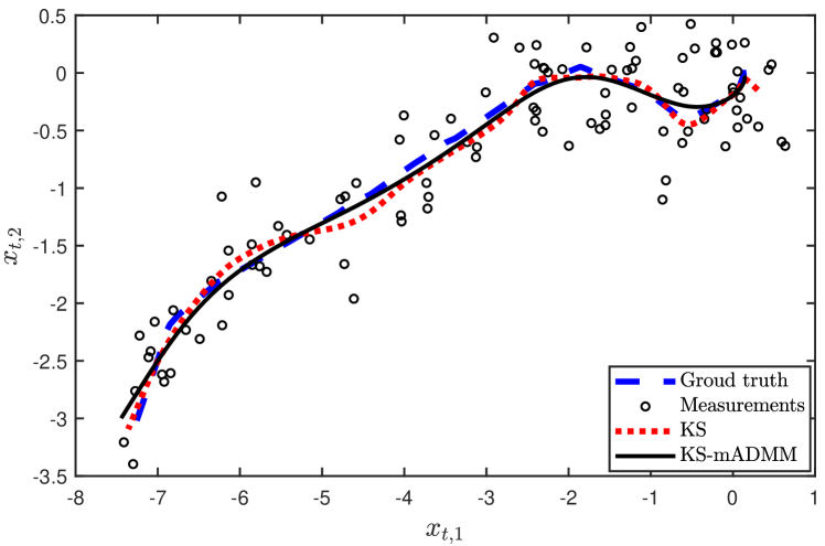
Refer to caption

Figure 1: Signals, measurements, and the estimates in the linear tracking problem. The values of 𝐱errsubscript𝐱err\mathbf{x}_{\text{err}} are 0.1030.1030.103 and 0.0720.0720.072 in KS and KS-mADMM, respectively.

Recall that the difference in batch and recursive ADMM running time is dominated by the 𝐱1:Tsubscript𝐱:1𝑇\mathbf{x}_{1:T}-subproblem. Fig. 2 demonstrates how the running time (sec) grows when T𝑇T is increasing. Despite being mathematically equivalent, mADMM and KS-mADMM, have very different running times. The running times of mADMM and prox-ADMM have a similar growth rate whereas KS-mADMM has a growth rate that resembles a plain Kalman smoother. Due to limited memory, we cannot report the results of the batch estimation methods (prox-ADMM and mADMM) when T>104𝑇superscript104T>10^{4}. At T=104𝑇superscript104T=10^{4}, the running times of KS, KS-mADMM, prox-ADMM, and mADMM, were 0.340.340.34s, 1.921.921.92s, 628462846284s and 964696469646s, respectively. The proposed method is computationally inexpensive, which makes it suitable for solving real-world applications, such as the marine vessel tracking in Section VI-C.
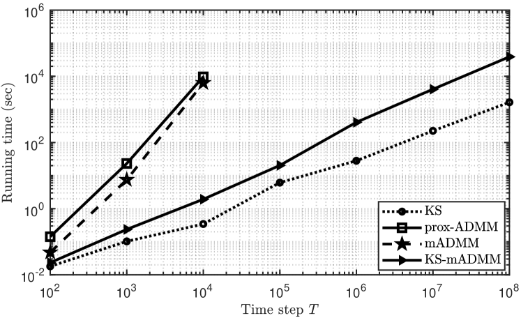
Refer to caption

Figure 2: Comparison of the running times in the linear car tracking example as function of the number of time steps.

VI-B Multi-Sensor Range Measurement Problems

In this experiment, we consider a multi-sensor range measurement problem where we have short periods of movement with regular stops. This problem frequently appears in many surveillance systems [6, 3]. The state 𝐱tsubscript𝐱𝑡\mathbf{x}_{t} contains the position (xt,1,xt,2)subscript𝑥𝑡1subscript𝑥𝑡2(x_{t,1},x_{t,2}) and the velocities (xt,3,xt,4)subscript𝑥𝑡3subscript𝑥𝑡4(x_{t,3},x_{t,4}). The measurement dynamic model for sensor n{1,2,3}𝑛123n\in\left\{1,2,3\right\} is given by

𝐡tn(𝐱t)=(xt,2syn)2+(xt,1sxn)2,superscriptsubscript𝐡𝑡𝑛subscript𝐱𝑡superscriptsubscript𝑥𝑡2superscriptsubscript𝑠𝑦𝑛2superscriptsubscript𝑥𝑡1superscriptsubscript𝑠𝑥𝑛2\mathbf{h}_{t}^{n}(\mathbf{x}_{t})=\sqrt{(x_{t,2}-s_{y}^{n})^{2}+(x_{t,1}-s_{x}^{n})^{2}},

where (sxn,syn)superscriptsubscript𝑠𝑥𝑛superscriptsubscript𝑠𝑦𝑛(s_{x}^{n},s_{y}^{n}) is the position of the sensor n𝑛n. The transition function 𝐚t(𝐱t1)subscript𝐚𝑡subscript𝐱𝑡1\mathbf{a}_{t}(\mathbf{x}_{t-1}) is

𝐚t(𝐱t1)=[10t0010t00100001]𝐱t1.subscript𝐚𝑡subscript𝐱𝑡1matrix10𝑡0010𝑡00100001subscript𝐱𝑡1\mathbf{a}_{t}(\mathbf{x}_{t-1})=\begin{bmatrix}1&0&\triangle t&0\\ 0&1&0&\triangle t\\ 0&0&1&0\\ 0&0&0&1\end{bmatrix}\,\mathbf{x}_{t-1}. (35)

The covariances are 𝐑t=diag(0.22,0.22)subscript𝐑𝑡diagsuperscript0.22superscript0.22\mathbf{R}_{t}=\operatorname{diag}(0.2^{2},0.2^{2}), and 𝐐t=diag(0.01,0.01,0.1,0.1)subscript𝐐𝑡diag0.010.010.10.1\mathbf{Q}_{t}=\operatorname{diag}(0.01,0.01,0.1,0.1). We set Δt=0.1Δ𝑡0.1\Delta t=0.1, T=60𝑇60T=60, (sx1,sy1)=(0,0.5)superscriptsubscript𝑠𝑥1superscriptsubscript𝑠𝑦100.5(s_{x}^{1},\,s_{y}^{1})=(0,-0.5), (sx2,sy2)=(0.5,0.6)superscriptsubscript𝑠𝑥2superscriptsubscript𝑠𝑦20.50.6(s_{x}^{2},\,s_{y}^{2})=(0.5,0.6), (sx3,sy3)=(0.5,0.6)superscriptsubscript𝑠𝑥3superscriptsubscript𝑠𝑦30.50.6(s_{x}^{3},s_{y}^{3})=(0.5,0.6), 𝐦1=[0000]subscript𝐦1superscriptmatrix0000top\mathbf{m}_{1}=\begin{bmatrix}0&0&0&0\end{bmatrix}^{\top}, and 𝐏1=𝐈/10subscript𝐏1𝐈10\mathbf{P}_{1}=\mathbf{I}/10. We assume the target has many stops, which means the velocities xt,3subscript𝑥𝑡3x_{t,3}, xt,4subscript𝑥𝑡4x_{t,4} are sparse. We also set 𝐆g,t=[𝟎𝐈],subscript𝐆𝑔𝑡matrix0𝐈\mathbf{G}_{g,t}=\begin{bmatrix}\mathbf{0}&\mathbf{I}\end{bmatrix}, and use the parameters γ=1𝛾1\gamma=1, μ=1𝜇1\mu=1, Kmax=50subscript𝐾50K_{\max}=50, and Imax=5subscript𝐼5I_{\max}=5. We plot the velocity variable xt,3subscript𝑥𝑡3x_{t,3} corresponding to the time step t𝑡t in Fig. 3, which indicates that our method (black line) can generate much more sparse results than the IEKS estimate (red dash line).
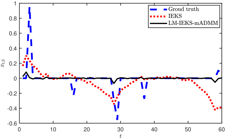
Refer to caption

Figure 3: The estimated trajectory in the nonlinear system. The relative errors are 0.530.530.53 and 0.460.460.46 generated by IEKS and LM-IEKS-ADMM.

Fig. 4 shows the relative error 𝐱errsubscript𝐱err\mathbf{x}_{\text{err}} as a function of the iteration number. The values of 𝐱errsubscript𝐱err\mathbf{x}_{\text{err}} generated by the regularisation methods are below those generated by iterated extended Kalman smoother (IEKS) [1]. It also shows that the GN-mADMM, GN-IEKS-mADMM, LM-mADMM and LM-IEKS-mADMM can find the optimal values in around 505050 iterations. IEKS is the fastest method, but the relative error is highest due to lack of the sparsity prior (i.e., μ=0𝜇0\mu=0). GN-mADMM and GN-IEKS-mADMM have the same convergence results (as they are equivalent), while the latter uses the less running time. Similarly, LM-mADMM and LM-IEKS-mADMM have the same convergence results, but LM-IEKS-mADMM needs less time to obtain the result than LM-mADMM. When the number of time steps T𝑇T is moderate, all the running time are acceptable. But when T𝑇T is extremely large, the proposed methods provide a massive advantage.
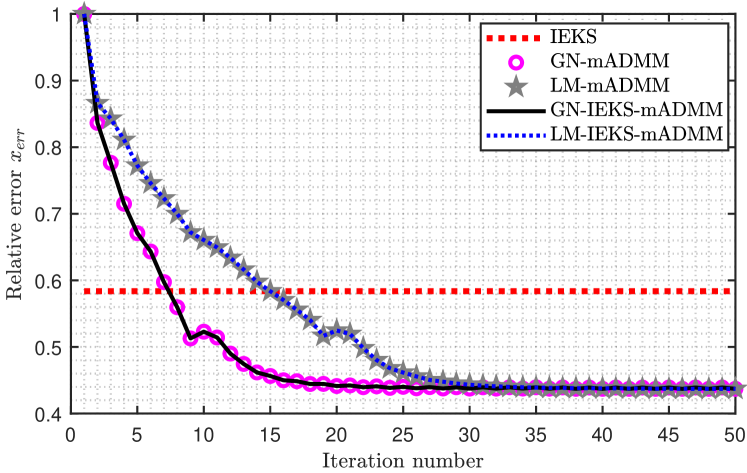
Refer to caption

Figure 4: Relative error 𝐱errsubscript𝐱err\mathbf{x}_{\text{err}} versus iteration number.

Fig. 5 demonstrates how the running time (sec) grows when T𝑇T is increasing. The proposed methods are compared with the state-of-the-art methods, including the proximal ADMM (prox-ADMM) [46], mADMM [47], and IEKS [1]. Despite being mathematically equivalent, GN-mADMM and GN-IEKS-mADMM, LM-mADMM and LM-IEKS-mADMM, have very different running times. GN-IEKS-mADMM and LM-IEKS-mADMM are more efficient than the batch methods. Due to limited memory, we cannot report the results of the batch methods when T>104𝑇superscript104T>10^{4}. It is reasonable to conclude that in general, the proposed methods are competitive for extremely large-scale tracking and estimation problems. The proposed approaches are computationally inexpensive, which makes them suitable for solving real-world applications, such as ship trajectory-tracking in the next section.
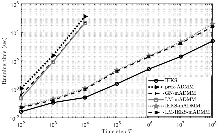
Refer to caption

Figure 5: Comparison of the running times in the range measurement example as function of the number of time steps (from 102superscript10210^{2} to 108superscript10810^{8}).

VI-C Marine Vessel Tracking

In this experiment, we utilise the Wiener velocity model [6] with a sparse noise assumption to track a marine vessel trajectory. The latitude, longitude, speed, and course of the vessel have been captured by automatic identification system (AIS) equipment, collected by Danish Maritime Authority. Similar applications can be found in [5, 39]. The state of the ship is measured at time intervals of 111 minute. Matrices 𝐇tsubscript𝐇𝑡\mathbf{H}_{t}, 𝐀tsubscript𝐀𝑡\mathbf{A}_{t}, 𝐐tsubscript𝐐𝑡\mathbf{Q}_{t}, and 𝐑tsubscript𝐑𝑡\mathbf{R}_{t} are the same with the settings in Section VI-A with Δt=1Δ𝑡1\Delta t=1, qc=1subscript𝑞𝑐1q_{c}=1, σ=0.3𝜎0.3\sigma=0.3, T=100𝑇100T=100, 𝐦1=[0.10.100]subscript𝐦1superscriptmatrix0.10.100top\mathbf{m}_{1}=\begin{bmatrix}0.1&0.1&0&0\end{bmatrix}^{\top}, and 𝐏1=100𝐈subscript𝐏1100𝐈\mathbf{P}_{1}=100\mathbf{I}. We assume the process noise 𝐪tsubscript𝐪𝑡\mathbf{q}_{t} is sparse, and set 𝐆g,tsubscript𝐆𝑔𝑡\mathbf{G}_{g,t} to an identity matrix and use the parameters γ=1𝛾1\gamma=1, μ=1𝜇1\mu=1, and Kmax=100subscript𝐾100K_{\max}=100. The measurement data consists of 100100100 time points of the vessel locations.

Our method obtains the position (latitude and longitude) estimates as shown in Fig. 6. Fig. 7 shows that our method has sparser process noise than estimated by the Kalman smoother (KS) [1]. We then highlight the computation advantage of our method. The difference in running time is dominated by the 𝐱1:Tsubscript𝐱:1𝑇\mathbf{x}_{1:T}-subproblem. The running times of KS, prox-ADMM, mADMM, and KS-mADMM, were 0.340.340.34s, 174174174s, 172172172s, and 5.635.635.63s, respectively. The running times of mADMM and prox-ADMM are similar whereas KS-mADMM has a smaller running time that resembles the plain Kalman smoother.
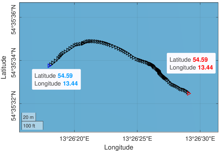
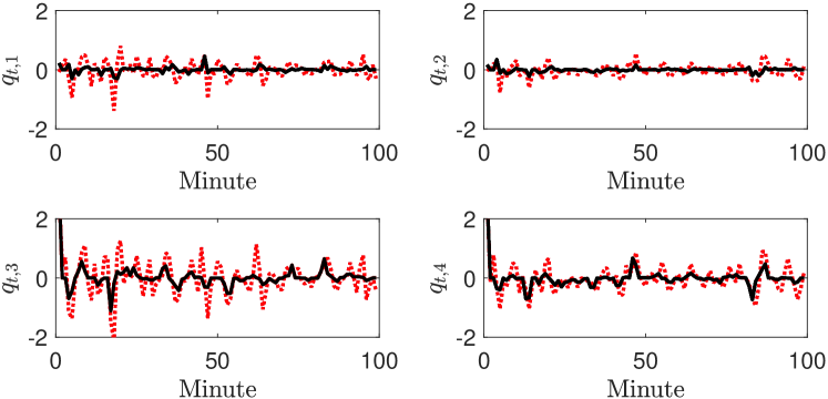
Refer to caption

Figure 6: The position (black markers) estimated by KS-mADMM. The starting coordinate is denoted blue marker, and the ending coordinate is red marker. Contains data from the Danish Maritime Authority that is used in accordance with the conditions for the use of Danish public data.

Refer to caption

Figure 7: The process noise estimated by KS-mADMM (black line) and Kalman smoother (red dash line).

VI-D Autonomous Vehicle Tracking

To further show how our methods can speed up larger scale real-world problems, we apply GN-IEKS-mADMM to a vehicle tracking problem using real-world data. Global positioning system (GPS) data was collected in urban streets and roads around Helsinki, Tuusula, and Vantaa, Finland [58]. The urban environment contained many stops to traffic lights, crossings, turns, and various other situations. We ran the experiment using a coordinate turn model [1], where the state at time step t𝑡t had the positions (xt,1,xt,2)subscript𝑥𝑡1subscript𝑥𝑡2(x_{t,1},\,x_{t,2}), the velocities (xt,3,xt,4)subscript𝑥𝑡3subscript𝑥𝑡4(x_{t,3},\,x_{t,4}), and the angular velocity xt,5subscript𝑥𝑡5x_{t,5}. The number of time points T𝑇T was 686568656865. We use the parameters γ=0.1𝛾0.1\gamma=0.1, μ=1𝜇1\mu=1, Kmax=300subscript𝐾300K_{\max}=300, Imax=5subscript𝐼5I_{\max}=5, 𝐦1=[4.513.5000]subscript𝐦1superscriptmatrix4.513.5000top\mathbf{m}_{1}=\begin{bmatrix}4.5&13.5&0&0&0\end{bmatrix}^{\top}, and 𝐏1=diag(50,50,50,50,0.01)subscript𝐏1diag505050500.01\mathbf{P}_{1}=\operatorname{diag}(50,50,50,50,0.01). We utilised the matrix

𝐆g,t=[001000001000001],subscript𝐆𝑔𝑡matrix001000001000001\mathbf{G}_{g,t}=\begin{bmatrix}0&0&1&0&0\\ 0&0&0&1&0\\ 0&0&0&0&1\end{bmatrix},

to enforce the sparsity of the velocities and the angular velocity.

The plot in Fig. 8 demonstrates the path (black line) generated by our method. The running time of IEKS [32], GN-mADMM, and GN-IEKS-mADMM were 222222s, 135201352013520s and 270427042704s, respectively. As we expected, although IEKS is fastest, the L2subscript𝐿2L_{2}-penalised regularisation methods push more of the velocities and the angle to zero, which is shown in Fig. 9. The IEKS estimate has many large peaks that appear as a result of large residuals, and GN-IEKS-mADMM has more sparse results.
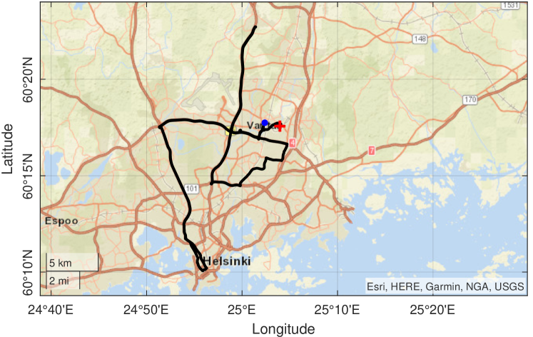
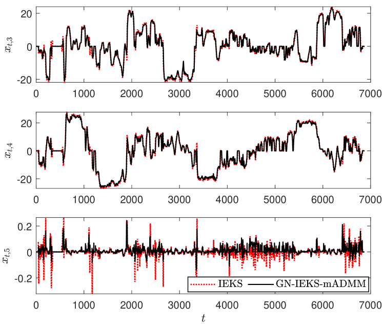
Refer to caption

Figure 8: The path tracking (black line) generated by GN-IEKS-mADMM. The starting position is blue point, and the ending position is red cross.

Refer to caption

Figure 9: The estimated velocities and angular velocities generated by IEKS (red dash line) and the proposed method (black line).

VI-E Audio Signal Restoration

The proposed technique can be readily applied to the problem of noise reduction in audio signals. We adopt a Gabor regression model [19]:

y(τ)=m=0M/2n=0N1cm,ngm,n(τ)+r(τ),τ=0,,T1,formulae-sequence𝑦𝜏superscriptsubscript𝑚0𝑀2superscriptsubscript𝑛0𝑁1subscript𝑐𝑚𝑛subscript𝑔𝑚𝑛𝜏𝑟𝜏𝜏0𝑇1y(\tau)=\sum_{m=0}^{M/2}\sum_{n=0}^{N-1}c_{m,n}g_{m,n}(\tau)+r(\tau),~{}~{}~{}~{}\tau=0,\dots,T-1,

where signals are represented as a weighted sum of Gabor atoms gm,n(τ)=wn(τ)exp(2πimMτ)subscript𝑔𝑚𝑛𝜏subscript𝑤𝑛𝜏2𝜋i𝑚𝑀𝜏g_{m,n}(\tau)=~{}w_{n}(\tau)\exp\left(2\pi\mathrm{i}\frac{m}{M}\tau\right). Terms wn(τ)subscript𝑤𝑛𝜏w_{n}(\tau) correspond to a window function with bounded support centred at time instants τnsubscript𝜏𝑛\tau_{n} (windows are placed so that the time axis is with tiled evenly). Sparsity is promoted through the L21superscriptsubscript𝐿21L_{2}^{1} pair-wise grouping pattern described in Section II: m,nμm,ncm,n2subscript𝑚𝑛subscript𝜇𝑚𝑛subscriptnormsubscript𝑐𝑚𝑛2\sum_{m,n}\mu_{m,n}\|c_{m,n}\|_{2}. The real representation of complex coefficients cm,nsubscript𝑐𝑚𝑛c_{m,n} used in [19] is adopted. This batch problem is restated in terms of a state-space model: signal 𝐲𝐲\mathbf{y} is separated into P𝑃P chunks 𝐲tsubscript𝐲𝑡\mathbf{y}_{t} of length L𝐿L and state vectors 𝐱t=[𝐜2(t1);𝐜2t1;𝐜2t]subscript𝐱𝑡superscriptsubscript𝐜2𝑡1subscript𝐜2𝑡1subscript𝐜2𝑡top\mathbf{x}_{t}=[\mathbf{c}_{2(t-1)};\mathbf{c}_{2t-1};\mathbf{c}_{2t}]^{\top} are defined, 𝐜tsubscript𝐜𝑡\mathbf{c}_{t} being the subvector associated to each frame. Let 𝐇0subscript𝐇0\mathbf{H}_{0} be a matrix containing the non-zero values of the Gabor basis functions 𝐠0,0,,𝐠M/2,0subscript𝐠00subscript𝐠𝑀20\mathbf{g}_{0,0},\dots,\mathbf{g}_{M/2,0} as columns. Thus, atoms in subsequent frames are time-shifted replicas of this basic set and 𝐲𝐃𝐜2superscriptnorm𝐲𝐃𝐜2\|\mathbf{y}-\mathbf{D}\mathbf{c}\|^{2} (𝐃𝐃\mathbf{D} a dictionary matrix containing all atoms) can be replaced by t=1P𝐲t𝐇𝐱t2superscriptsubscript𝑡1𝑃superscriptnormsubscript𝐲𝑡subscript𝐇subscript𝐱𝑡2\sum_{t=1}^{P}\|\mathbf{y}_{t}-\mathbf{H_{\ast}}\mathbf{x}_{t}\|^{2} +t=1P𝐱t𝐀t𝐱t12superscriptsubscript𝑡1𝑃superscriptnormsubscript𝐱𝑡subscript𝐀𝑡subscript𝐱𝑡12+\sum_{t=1}^{P}\|\mathbf{x}_{t}-\mathbf{A}_{t}\mathbf{x}_{t-1}\|^{2}, with 𝐇=[𝐇u𝐇0𝐇]subscript𝐇matrixsubscript𝐇𝑢subscript𝐇0subscript𝐇\mathbf{H}_{\ast}=\begin{bmatrix}\mathbf{H}_{u}&\mathbf{H}_{0}&\mathbf{H}_{\ell}\end{bmatrix} and 𝐀t=[𝟎𝟎𝟎;𝟎𝟎𝟎;𝐈𝟎𝟎]subscript𝐀𝑡matrix000000𝐈00\mathbf{A}_{t}=\begin{bmatrix}\mathbf{0}&\mathbf{0}&\mathbf{0};\quad\mathbf{0}&\mathbf{0}&\mathbf{0};\quad\mathbf{I}&\mathbf{0}&\mathbf{0}\end{bmatrix}. Terms 𝐇u,𝐇subscript𝐇𝑢subscript𝐇\mathbf{H}_{u},\mathbf{H}_{\ell} are truncated versions of 𝐇0subscript𝐇0\mathbf{H}_{0} corresponding to the contribution of the adjacent overlapping frames.

The algorithm is tested on a similar-to\sim3 second long glockenspiel excerpt sampled at 22050 [Hz] and contaminated with artificial background noise with signal-to-noise ratio (SNR) 5dB5dB5\text{dB}. Experiments are carried out in an Intel Core i7 @ 2.50GHz, 16 GB RAM, with parameters γ=5𝛾5\gamma=5, μ=2.6𝜇2.6\mu=2.6, and Kmax=500subscript𝐾500K_{\max}=500 and a window length L=512𝐿512L=512. Kalman gain matrices are precomputed. Reflecting the power spectrum of typical audio signals, which decays with frequency, penalisation is made frequency-dependent by setting μm,n=μ/f(m)subscript𝜇𝑚𝑛𝜇𝑓𝑚\mu_{m,n}=\mu/f(m), with f(m)𝑓𝑚f(m) a decreasing modulating function (e.g., a Butterworth filter gain), in a similar fashion to [18]. Coefficients are initialised at zero.The average output SNR is 12.412.412.4 with an average running time of 64.664.664.6s in 20 realisations. Fig. 10 shows the visual reconstruction results.

In comparison, Gibbs sampling schemes for models (e.g., [19]) yield noisier restorations with comparable computing times. We analysed the same example using the Gibbs sampler with 500 iterations, 250 burn-in period. Hyperparameters and initial values are chosen to ensure a fair comparison with the KS-mADMM method (unfavorable initialisation may induce longer convergence times). With a runtime of similar-to\sim180 seconds, the Gibbs algorithm yields an output SNR of similar-to\sim15 dB. The Perceptual Evaluation of Audio Quality (PEAQ) [59], a measure that incorporates psycho-acoustic criteria to asses audio signals, is adopted. The Objective Difference Grade (ODG) indicator derived from PEAQ is used to compare the reconstructions with respect to the clean reference signal, obtaining ODG = 3.9103.910-3.910 for clean signal against noisy input, ODG = 3.8463.846-3.846 for clean signal against Gibbs reconstruction, and ODG = 3.6373.637-3.637 for clean signal against KS-mADMM reconstruction (the closer to 0, the better). Despite the lower SNR (12.4 dB), the KS-ADMM reconstruction sounds cleaner (i.e., has fewer audio artefacts) than its Gibbs counterpart, which is consistent with the ODG values obtained. Devising appropriate temporal evolution models for the audio synthesis coefficients over time and investigating self-adaptive schemes for the estimation of μ𝜇\mu (here tuned empirically) are topics of future research.
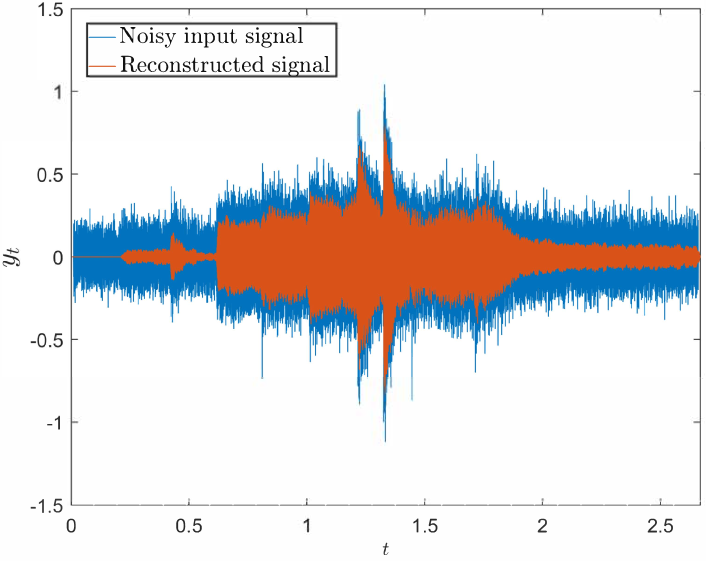
Refer to caption

Figure 10: Reconstructed glockenspiel excerpt.

VII Conclusion and Discussion

In this paper, we have presented efficient smoothing-and-splitting methods for solving regularised autonomous tracking and state estimation problems. We formulated the problem as a generalised L2subscript𝐿2L_{2}-penalised dynamic group Lasso minimisation problem. The problem can be solved using batch methods when the number of time steps is moderate. For the case with a large number of time steps, new KS-mADMM, GN-IEKS-mADMM, and LM-IEKS-mADMM methods were developed. We also proved the convergence of the proposed methods. We applied the developed methods to simulated tracking, real-world tracking, and audio signal restoration problems, where methods resulted in improved localisation and estimation performance and significantly reduced computation load.

A disadvantage of the smoothing-and-splitting methods is that although the methods significantly improve the tracking and estimation performance, their reliability depends on user-defined penalty parameters (e.g., the parameter γ𝛾\gamma in (6)). See [47, 46] for further details on choosing the appropriate values of the parameters. The use of adaptive penalty parameters may improve the performance in dynamic systems, even while stronger conditions of convergence need to be guaranteed [60]. It would be interesting to develop fully automated solvers with adaptive parameters. The convergence and the convergence rate of our methods are based on Bayesian smoothers and ADMM, and we have established the convergence rate of the convex case. Possible future work includes discussing the convergence rate for nonconvex variants.

Although we only consider the autonomous tracking and state estimation problems in this paper, it is possible to apply our framework to a wide class of control problems. For example, in linear optimal control problems, we could introduce splitting variables to decompose the nonsmooth terms and then use the Riccati equations to compute the subproblems arising in the optimal control problems [61]. In cooperative control of multiple target systems [62, 63, 64], we can consider a reformulation of dynamic models of group targets into classes with different characteristics. Based on the framework, we address the subproblems in implementing optimisation-based methods such as receding horizon methods [63]. The proposed framework can be extended to other variable splitting methods [48] as well as other recursive smoothers [1]. Future work also includes developing other variants, for example, sigma-point based variable splitting methods.

Appendix A Proof of Lemma 1

For proving Lemma 1, we define 𝜻=[𝐱𝐰]𝜻superscriptmatrix𝐱𝐰top\bm{\zeta}=\begin{bmatrix}\mathbf{x}&\mathbf{w}\end{bmatrix}^{\top} and then write variables 𝐱𝐱\mathbf{x} and 𝐰𝐰\mathbf{w} into the function Ξ(𝜻)Ξ𝜻\Xi(\bm{\zeta}), which is

Ξ(𝜻)=12𝐲𝐇𝐱𝐞𝐑12+12𝐦𝚽𝐱𝐛𝐐12+μ𝐰2.Ξ𝜻12superscriptsubscriptnorm𝐲𝐇𝐱𝐞superscript𝐑1212superscriptsubscriptnorm𝐦𝚽𝐱𝐛superscript𝐐12𝜇subscriptnorm𝐰2\Xi(\bm{\zeta})=\frac{1}{2}\left\|{\mathbf{y}}-\mathbf{H}\mathbf{x}-\mathbf{e}\right\|_{\mathbf{R}^{-1}}^{2}+\frac{1}{2}\left\|{\mathbf{m}}-\mathbf{\Phi}\mathbf{x}-\mathbf{b}\right\|_{\mathbf{Q}^{-1}}^{2}+\mu\left\|\mathbf{w}\right\|_{2}. (36)

Using the optimality conditions of the subproblems in (7), we can write

Ξ(𝜻)Ξ(𝜻(k+1))+(𝜻𝜻(k+1))([𝚽𝟎𝟎𝐈]𝜼(k)\displaystyle\Xi(\bm{\zeta})-\Xi(\bm{\zeta}^{(k+1)})+(\bm{\zeta}-\bm{\zeta}^{(k+1)})^{\top}\left(\begin{bmatrix}\mathbf{\Phi}&\mathbf{0}\\ \mathbf{0}&\mathbf{I}\end{bmatrix}^{\top}\bm{\eta}^{(k)}\right.
+γ[𝚽𝟎𝟎𝐈](𝜻(k+1)[𝐈𝐆]𝐯(k)[𝐝𝟎]))𝟎,\displaystyle\left.\quad+\gamma\begin{bmatrix}\mathbf{\Phi}&\mathbf{0}\\ \mathbf{0}&\mathbf{I}\end{bmatrix}^{\top}\big{(}\bm{\zeta}^{(k+1)}-\begin{bmatrix}\mathbf{I}\\ \mathbf{G}\end{bmatrix}\mathbf{v}^{(k)}-\begin{bmatrix}\mathbf{d}\\ \mathbf{0}\end{bmatrix}\big{)}\right)\geq\mathbf{0}, (37a)
(𝐯𝐯(k+1))([𝐈𝐆]𝜼(k)\displaystyle(\mathbf{v}-\mathbf{v}^{(k+1)})^{\top}\left(-\begin{bmatrix}\mathbf{I}\\ \mathbf{G}\end{bmatrix}^{\top}\bm{\eta}^{(k)}\right.
γ[𝐈𝐆](𝜻(k+1)[𝐈𝐆]𝐯(k+1)[𝐝𝟎]))𝟎,\displaystyle\left.\quad-\gamma\begin{bmatrix}\mathbf{I}\\ \mathbf{G}\end{bmatrix}^{\top}\big{(}\bm{\zeta}^{(k+1)}-\begin{bmatrix}\mathbf{I}\\ \mathbf{G}\end{bmatrix}\mathbf{v}^{(k+1)}-\begin{bmatrix}\mathbf{d}\\ \mathbf{0}\end{bmatrix}\big{)}\right)\geq\mathbf{0}, (37b)
(𝜼𝜼(k+1))(([𝚽𝟎𝟎𝐈]𝐳(k+1)[𝐈𝐆]𝐯(k+1)[𝐝𝟎])\displaystyle(\bm{\eta}-\bm{\eta}^{(k+1)})^{\top}\left(-\big{(}\begin{bmatrix}\mathbf{\Phi}&\mathbf{0}\\ \mathbf{0}&\mathbf{I}\end{bmatrix}\mathbf{z}^{(k+1)}-\begin{bmatrix}\mathbf{I}\\ \mathbf{G}\end{bmatrix}\mathbf{v}^{(k+1)}-\begin{bmatrix}\mathbf{d}\\ \mathbf{0}\end{bmatrix}\big{)}\right.
+1γ(𝜼(k+1)𝜼(k)))𝟎.\displaystyle\left.\quad+\frac{1}{\gamma}(\bm{\eta}^{(k+1)}-\bm{\eta}^{(k)})\right)\geq\mathbf{0}. (37c)

For simplicity of notation, we also define

𝝃=[𝜻𝐯𝜼],F(𝝃)=[[𝚽𝟎𝟎𝐈]𝜼(k+1)[𝐈𝐆]𝜼(k+1)[𝚽𝟎𝟎𝐈]𝜻(k+1)+[𝐈𝐆]𝐯(k+1)+[𝐝𝟎]].𝝃absentsuperscriptmatrix𝜻𝐯𝜼top𝐹𝝃absentmatrixsuperscriptmatrix𝚽00𝐈topsuperscript𝜼𝑘1superscriptmatrix𝐈𝐆topsuperscript𝜼𝑘1matrix𝚽00𝐈superscript𝜻𝑘1matrix𝐈𝐆superscript𝐯𝑘1matrix𝐝0\begin{split}\begin{aligned} \bm{\xi}&=\begin{bmatrix}\bm{\zeta}&\mathbf{v}&\bm{\eta}\end{bmatrix}^{\top},\\ F(\bm{\xi})&=\begin{bmatrix}\begin{bmatrix}\mathbf{\Phi}&\mathbf{0}\\ \mathbf{0}&\mathbf{I}\end{bmatrix}^{\top}\bm{\eta}^{(k+1)}\\ -\begin{bmatrix}\mathbf{I}\\ \mathbf{G}\end{bmatrix}^{\top}\bm{\eta}^{(k+1)}\\ -\begin{bmatrix}\mathbf{\Phi}&\mathbf{0}\\ \mathbf{0}&\mathbf{I}\end{bmatrix}\bm{\zeta}^{(k+1)}+\begin{bmatrix}\mathbf{I}\\ \mathbf{G}\end{bmatrix}\mathbf{v}^{(k+1)}+\begin{bmatrix}\mathbf{d}\\ \mathbf{0}\end{bmatrix}\\ \end{bmatrix}.\end{aligned}\end{split} (38)

We group all the variables 𝜻𝜻\bm{\zeta}, 𝐯𝐯\mathbf{v}, and 𝜼𝜼\bm{\eta} into a single vector 𝝃𝝃\bm{\xi}, and then rewrite (37) as follows:

Ξ(𝜻)Ξ(𝜻(k+1))+[𝝃𝝃(k+1)](F(𝝃)+γ[[𝚽𝟎𝟎𝐈][𝐈𝐆]𝟎][𝐈𝐆](𝐯(k)𝐯(k+1))+[𝟎𝟎γ[𝐈𝐆]𝟎𝟎1γ𝐈][𝐯(k+1)𝐯(k)𝜼(k+1)𝜼(k)])𝟎,Ξ(𝜻)Ξ(𝜻(k+1))+[𝝃𝝃(k+1)]F(𝝃)+γ[𝝃𝝃(k+1)][[𝚽𝟎𝟎𝐈][𝐈𝐆]𝟎][𝐈𝐆](𝐯(k)𝐯(k+1))[𝐯𝐯(k+1)𝜼𝜼(k+1)][γ[𝐈𝐆]𝟎𝟎1γ𝐈][𝐯(k+1)𝐯(k)𝜼(k+1)𝜼(k)].\begin{split}\begin{aligned} &\Xi(\bm{\zeta})-\Xi(\bm{\zeta}^{(k+1)})+\begin{bmatrix}\bm{\xi}-\bm{\xi}^{(k+1)}\\ \end{bmatrix}^{\top}\\ &\quad\left(F(\bm{\xi})+\gamma\begin{bmatrix}\begin{bmatrix}\mathbf{\Phi}&\mathbf{0}\\ \mathbf{0}&\mathbf{I}\end{bmatrix}^{\top}\\ -\begin{bmatrix}\mathbf{I}\\ \mathbf{G}\end{bmatrix}^{\top}\\ \mathbf{0}\\ \end{bmatrix}\begin{bmatrix}\mathbf{I}\\ \mathbf{G}\end{bmatrix}(\mathbf{v}^{(k)}-\mathbf{v}^{(k+1)})\right.\\ &\left.\qquad+\begin{bmatrix}&\mathbf{0}&\mathbf{0}\\ &\gamma\begin{bmatrix}\mathbf{I}\\ \mathbf{G}\end{bmatrix}^{\top}&\mathbf{0}\\ &\mathbf{0}&\frac{1}{\gamma}\mathbf{I}\\ \end{bmatrix}\begin{bmatrix}\mathbf{v}^{(k+1)}-\mathbf{v}^{(k)}\\ \bm{\eta}^{(k+1)}-\bm{\eta}^{(k)}\\ \end{bmatrix}\right)\geq\mathbf{0},\\ &\Xi(\bm{\zeta})-\Xi(\bm{\zeta}^{(k+1)})+\begin{bmatrix}\bm{\xi}-\bm{\xi}^{(k+1)}\\ \end{bmatrix}^{\top}F(\bm{\xi})\\ &\quad+\gamma\begin{bmatrix}\bm{\xi}-\bm{\xi}^{(k+1)}\\ \end{bmatrix}^{\top}\begin{bmatrix}\begin{bmatrix}\mathbf{\Phi}&\mathbf{0}\\ \mathbf{0}&\mathbf{I}\end{bmatrix}^{\top}\\ -\begin{bmatrix}\mathbf{I}\\ \mathbf{G}\end{bmatrix}^{\top}\\ \mathbf{0}\\ \end{bmatrix}\begin{bmatrix}\mathbf{I}\\ \mathbf{G}\end{bmatrix}\big{(}\mathbf{v}^{(k)}-\mathbf{v}^{(k+1)}\big{)}\\ &\quad\geq\begin{bmatrix}\mathbf{v}-\mathbf{v}^{(k+1)}\\ \bm{\eta}-\bm{\eta}^{(k+1)}\\ \end{bmatrix}^{\top}\begin{bmatrix}&\gamma\begin{bmatrix}\mathbf{I}\\ \mathbf{G}\end{bmatrix}^{\top}&\mathbf{0}\\ &\mathbf{0}&\frac{1}{\gamma}\mathbf{I}\\ \end{bmatrix}\begin{bmatrix}\mathbf{v}^{(k+1)}-\mathbf{v}^{(k)}\\ \bm{\eta}^{(k+1)}-\bm{\eta}^{(k)}\\ \end{bmatrix}.\end{aligned}\end{split} (39)

Since the mapping F(𝝃)𝐹𝝃F(\bm{\xi}) is affine with a skew-symmetric matrix, it is monotonic [52]. Then we have the inequality

Ξ(𝜻(k+1))Ξ(𝜻)+(𝝃(k+1)𝝃)F(𝝃(k+1))Ξ(𝜻(k+1))Ξ(𝜻)+(𝝃(k+1)𝝃)F(𝝃)𝟎.missing-subexpressionΞsuperscript𝜻𝑘1Ξsuperscript𝜻superscriptsuperscript𝝃𝑘1superscript𝝃top𝐹superscript𝝃𝑘1missing-subexpressionabsentΞsuperscript𝜻𝑘1Ξsuperscript𝜻superscriptsuperscript𝝃𝑘1superscript𝝃top𝐹superscript𝝃0\begin{split}\begin{aligned} &\Xi(\bm{\zeta}^{(k+1)})-\Xi(\bm{\zeta}^{\star})+(\bm{\xi}^{(k+1)}-\bm{\xi}^{\star})^{\top}F(\bm{\xi}^{(k+1)})\\ &\geq\Xi(\bm{\zeta}^{(k+1)})-\Xi(\bm{\zeta}^{\star})+(\bm{\xi}^{(k+1)}-\bm{\xi}^{\star})^{\top}F(\bm{\xi}^{\star})\geq\mathbf{0}.\end{aligned}\end{split} (40)

Meanwhile, using (7d), the inequality can be written as

(𝜼(k)𝜼(k+1))([𝐈𝐆])(𝐯(k)𝐯(k+1))𝟎.superscriptsuperscript𝜼𝑘superscript𝜼𝑘1topmatrix𝐈𝐆superscript𝐯𝑘superscript𝐯𝑘10\begin{split}\begin{aligned} (\bm{\eta}^{(k)}-\bm{\eta}^{(k+1)})^{\top}\left(-\begin{bmatrix}\mathbf{I}\\ \mathbf{G}\\ \end{bmatrix}\right)(\mathbf{v}^{(k)}-\mathbf{v}^{(k+1)})\geq\mathbf{0}.\end{aligned}\end{split} (41)

Combing (40) and (41), we can derive (39) as

([𝐯(k+1)𝜼(k+1)][𝐯𝜼])[γ𝐈+𝐆𝐆𝟎𝟎1γ𝐈]([𝐯(k)𝜼(k)][𝐯(k+1)𝜼(k+1)])γ[𝝃(k+1)𝝃][[𝚽𝟎𝟎𝐈][𝐈𝐆]𝟎][𝐈𝐆](𝐯(k)𝐯(k+1))(𝜼(k)𝜼(k+1))([𝐈𝐆])(𝐯(k)𝐯(k+1))𝟎.missing-subexpressionsuperscriptmatrixsuperscript𝐯𝑘1superscript𝜼𝑘1matrixsuperscript𝐯superscript𝜼topmatrix𝛾𝐈superscript𝐆top𝐆001𝛾𝐈matrixsuperscript𝐯𝑘superscript𝜼𝑘matrixsuperscript𝐯𝑘1superscript𝜼𝑘1missing-subexpressionabsent𝛾superscriptmatrixsuperscript𝝃𝑘1superscript𝝃topmatrixsuperscriptmatrix𝚽00𝐈topsuperscriptmatrix𝐈𝐆top0matrix𝐈𝐆superscript𝐯𝑘superscript𝐯𝑘1missing-subexpressionabsentsuperscriptsuperscript𝜼𝑘superscript𝜼𝑘1topmatrix𝐈𝐆superscript𝐯𝑘superscript𝐯𝑘10\begin{split}\begin{aligned} &\left(\begin{bmatrix}\mathbf{v}^{(k+1)}\\ \bm{\eta}^{(k+1)}\\ \end{bmatrix}-\begin{bmatrix}\mathbf{v}^{\star}\\ \bm{\eta}^{\star}\\ \end{bmatrix}\right)^{\top}\begin{bmatrix}\gamma\mathbf{I}+{\mathbf{G}}^{\top}{\mathbf{G}}&\mathbf{0}\\ \mathbf{0}&\frac{1}{\gamma}\mathbf{I}\\ \end{bmatrix}\left(\begin{bmatrix}\mathbf{v}^{(k)}\\ \bm{\eta}^{(k)}\\ \end{bmatrix}-\begin{bmatrix}\mathbf{v}^{(k+1)}\\ \bm{\eta}^{(k+1)}\\ \end{bmatrix}\right)\\ &\geq\gamma\begin{bmatrix}\bm{\xi}^{(k+1)}-\bm{\xi}^{\star}\\ \end{bmatrix}^{\top}\begin{bmatrix}\begin{bmatrix}\mathbf{\Phi}&\mathbf{0}\\ \mathbf{0}&\mathbf{I}\end{bmatrix}^{\top}\\ -\begin{bmatrix}\mathbf{I}\\ \mathbf{G}\end{bmatrix}^{\top}\\ \mathbf{0}\\ \end{bmatrix}\begin{bmatrix}\mathbf{I}\\ \mathbf{G}\end{bmatrix}\big{(}\mathbf{v}^{(k)}-\mathbf{v}^{(k+1)}\big{)}\\ &\quad\geq(\bm{\eta}^{(k)}-\bm{\eta}^{(k+1)})^{\top}\left(-\begin{bmatrix}\mathbf{I}\\ \mathbf{G}\\ \end{bmatrix}\right)\big{(}\mathbf{v}^{(k)}-\mathbf{v}^{(k+1)}\big{)}\geq\mathbf{0}.\end{aligned}\end{split} (42)

Let 𝛀=[γ𝐈+𝐆𝐆𝟎𝟎1γ𝐈]𝛀matrix𝛾𝐈superscript𝐆top𝐆001𝛾𝐈\mathbf{\Omega}=\begin{bmatrix}\gamma\mathbf{I}+{\mathbf{G}}^{\top}{\mathbf{G}}&\mathbf{0}\\ \mathbf{0}&\frac{1}{\gamma}\mathbf{I}\\ \end{bmatrix}. We then conclude that

[𝐯(k)𝜼(k)][𝐯𝜼]𝛀2=[𝐯(k+1)𝜼(k+1)][𝐯𝜼]𝛀2+[𝐯(k)𝜼(k)][𝐯(k+1)𝜼(k+1)]𝛀2+2([𝐯(k+1)𝜼(k+1)][𝐯𝜼])𝛀([𝐯(k)𝜼(k)][𝐯(k+1)𝜼(k+1)])[𝐯(k+1)𝜼(k+1)][𝐯𝜼]𝛀2+[𝐯(k)𝜼(k)][𝐯(k+1)𝜼(k+1)]𝛀2.missing-subexpressionsuperscriptsubscriptnormmatrixsuperscript𝐯𝑘superscript𝜼𝑘matrixsuperscript𝐯superscript𝜼𝛀2missing-subexpressionabsentsuperscriptsubscriptnormmatrixsuperscript𝐯𝑘1superscript𝜼𝑘1matrixsuperscript𝐯superscript𝜼𝛀2superscriptsubscriptnormmatrixsuperscript𝐯𝑘superscript𝜼𝑘matrixsuperscript𝐯𝑘1superscript𝜼𝑘1𝛀2missing-subexpression2superscriptmatrixsuperscript𝐯𝑘1superscript𝜼𝑘1matrixsuperscript𝐯superscript𝜼top𝛀matrixsuperscript𝐯𝑘superscript𝜼𝑘matrixsuperscript𝐯𝑘1superscript𝜼𝑘1missing-subexpressionabsentsuperscriptsubscriptnormmatrixsuperscript𝐯𝑘1superscript𝜼𝑘1matrixsuperscript𝐯superscript𝜼𝛀2superscriptsubscriptnormmatrixsuperscript𝐯𝑘superscript𝜼𝑘matrixsuperscript𝐯𝑘1superscript𝜼𝑘1𝛀2\begin{split}\begin{aligned} &\left\|\begin{bmatrix}\mathbf{v}^{(k)}\\ \bm{\eta}^{(k)}\\ \end{bmatrix}-\begin{bmatrix}\mathbf{v}^{\star}\\ \bm{\eta}^{\star}\\ \end{bmatrix}\right\|_{\mathbf{\Omega}}^{2}\\ &=\left\|\begin{bmatrix}\mathbf{v}^{(k+1)}\\ \bm{\eta}^{(k+1)}\\ \end{bmatrix}-\begin{bmatrix}\mathbf{v}^{\star}\\ \bm{\eta}^{\star}\\ \end{bmatrix}\right\|_{\mathbf{\Omega}}^{2}+\left\|\begin{bmatrix}\mathbf{v}^{(k)}\\ \bm{\eta}^{(k)}\\ \end{bmatrix}-\begin{bmatrix}\mathbf{v}^{(k+1)}\\ \bm{\eta}^{(k+1)}\\ \end{bmatrix}\right\|_{\mathbf{\Omega}}^{2}\\ &\,+2\left(\begin{bmatrix}\mathbf{v}^{(k+1)}\\ \bm{\eta}^{(k+1)}\\ \end{bmatrix}-\begin{bmatrix}\mathbf{v}^{\star}\\ \bm{\eta}^{\star}\\ \end{bmatrix}\right)^{\top}\mathbf{\Omega}\left(\begin{bmatrix}\mathbf{v}^{(k)}\\ \bm{\eta}^{(k)}\\ \end{bmatrix}-\begin{bmatrix}\mathbf{v}^{(k+1)}\\ \bm{\eta}^{(k+1)}\\ \end{bmatrix}\right)\\ &\geq\left\|\begin{bmatrix}\mathbf{v}^{(k+1)}\\ \bm{\eta}^{(k+1)}\\ \end{bmatrix}-\begin{bmatrix}\mathbf{v}^{\star}\\ \bm{\eta}^{\star}\\ \end{bmatrix}\right\|_{\mathbf{\Omega}}^{2}+\left\|\begin{bmatrix}\mathbf{v}^{(k)}\\ \bm{\eta}^{(k)}\\ \end{bmatrix}-\begin{bmatrix}\mathbf{v}^{(k+1)}\\ \bm{\eta}^{(k+1)}\\ \end{bmatrix}\right\|_{\mathbf{\Omega}}^{2}.\end{aligned}\end{split} (43)

Appendix B Proof of Lemma 2

To simplify the notation, we replace the (k+1)::𝑘1absent(k+1): iteration by the ++:th iteration, and drop the iteration counter k𝑘k in this proof. Due to the strongly amenability, s(𝐱)𝑠𝐱s(\mathbf{x}) is prox-regular with a positive constant M𝑀M. Now we compute

γ(𝐱,𝐰,𝐯;𝜼)γ(𝐱(+),𝐰(+),𝐯;𝜼)=s(𝐱)s(𝐱(+))+𝜼¯,𝚽𝐱(+)𝚽𝐱+γ(𝚽𝐱(+)𝐝𝐯),𝚽𝐱(+)𝚽𝐱+γ2𝚽𝐱(+)𝚽𝐱2+g(𝐰)g(𝐰(+))+𝜼¯,𝐰(+)𝐰+γ(𝐰(+)𝐆𝐯),𝐰(+)𝐰+γ2𝐰(+)𝐰2>γδ+(𝚽𝚽)M2𝐱(+)𝐱2+γ2𝐰(+)𝐰2,subscript𝛾𝐱𝐰𝐯𝜼subscript𝛾superscript𝐱superscript𝐰𝐯𝜼𝑠𝐱𝑠superscript𝐱¯𝜼𝚽superscript𝐱𝚽𝐱𝛾𝚽superscript𝐱𝐝𝐯𝚽superscript𝐱𝚽𝐱𝛾2superscriptdelimited-∥∥𝚽superscript𝐱𝚽𝐱2𝑔𝐰𝑔superscript𝐰¯𝜼superscript𝐰𝐰𝛾superscript𝐰𝐆𝐯superscript𝐰𝐰𝛾2superscriptdelimited-∥∥superscript𝐰𝐰2𝛾subscript𝛿superscript𝚽top𝚽𝑀2superscriptdelimited-∥∥superscript𝐱𝐱2𝛾2superscriptdelimited-∥∥superscript𝐰𝐰2\begin{split}&\mathcal{L}_{\gamma}(\mathbf{x},\mathbf{w},\mathbf{v};\bm{\eta})-\mathcal{L}_{\gamma}(\mathbf{x}^{(+)},\mathbf{w}^{(+)},\mathbf{v};\bm{\eta})\\ &=s(\mathbf{x})-s(\mathbf{x}^{(+)})+\langle\overline{\bm{\eta}},\mathbf{\Phi}\mathbf{x}^{(+)}-\mathbf{\Phi}\mathbf{x}\rangle\\ &+\langle\gamma(\mathbf{\Phi}\mathbf{x}^{(+)}-\mathbf{d}-\mathbf{v}),\mathbf{\Phi}\mathbf{x}^{(+)}-\mathbf{\Phi}\mathbf{x}\rangle+\frac{\gamma}{2}\|\mathbf{\Phi}\mathbf{x}^{(+)}-\mathbf{\Phi}\mathbf{x}\|^{2}\\ &\quad+g(\mathbf{w})-g(\mathbf{w}^{(+)})+\langle\underline{\bm{\eta}},\mathbf{w}^{(+)}-\mathbf{w}\rangle\\ &\qquad+\langle\gamma(\mathbf{w}^{(+)}-\mathbf{G}\mathbf{v}),\mathbf{w}^{(+)}-\mathbf{w}\rangle+\frac{\gamma}{2}\|\mathbf{w}^{(+)}-\mathbf{w}\|^{2}\\ &{>}\frac{\gamma\delta_{+}(\mathbf{\Phi}^{\top}\mathbf{\Phi})-M}{2}\|\mathbf{x}^{(+)}-\mathbf{x}\|^{2}+\frac{\gamma}{2}\|\mathbf{w}^{(+)}-\mathbf{w}\|^{2},\end{split} (44)

where 𝜼=vec(𝜼¯,𝜼¯)𝜼vec¯𝜼¯𝜼\bm{\eta}=\operatorname{vec}(\overline{\bm{\eta}},\underline{\bm{\eta}}). We then have

γ(𝐱(+),𝐰(+),𝐯(+);𝜼(+))γ(𝐱,𝐰,𝐯;𝜼)<1γ𝜼(+)𝜼2+Mγδ+(𝚽𝚽)2𝐱(+)𝐱2+γ2𝐰(+)𝐰2,missing-subexpressionsubscript𝛾superscript𝐱superscript𝐰superscript𝐯superscript𝜼subscript𝛾𝐱𝐰𝐯𝜼1𝛾superscriptnormsuperscript𝜼𝜼2missing-subexpression𝑀𝛾subscript𝛿superscript𝚽top𝚽2superscriptnormsuperscript𝐱𝐱2𝛾2superscriptnormsuperscript𝐰𝐰2\begin{split}\begin{aligned} &\mathcal{L}_{\gamma}(\mathbf{x}^{(+)},\mathbf{w}^{(+)},\mathbf{v}^{(+)};\bm{\eta}^{(+)})-\mathcal{L}_{\gamma}(\mathbf{x},\mathbf{w},\mathbf{v};\bm{\eta})<\frac{1}{\gamma}\|\bm{\eta}^{(+)}-\bm{\eta}\|^{2}\\ &+\frac{M-\gamma\delta_{+}(\mathbf{\Phi}^{\top}\mathbf{\Phi})}{2}\|\mathbf{x}^{(+)}-\mathbf{x}\|^{2}+\frac{\gamma}{2}\|\mathbf{w}^{(+)}-\mathbf{w}\|^{2},\end{aligned}\end{split} (45)

which will be nonnegative provided when γ>Mδ+(𝚽𝚽)>0𝛾𝑀subscript𝛿superscript𝚽top𝚽0\gamma>\frac{M}{\delta_{+}(\mathbf{\Phi}^{\top}\mathbf{\Phi})}>0 is satisfied. In particular, when 𝚽=𝐈𝚽𝐈\mathbf{\Phi}=\mathbf{I}, δ+(𝚽𝚽)=1subscript𝛿superscript𝚽top𝚽1\delta_{+}(\mathbf{\Phi}^{\top}\mathbf{\Phi})=1.

In our case, γ(𝐱(k),𝐰(k),𝐯(k);𝜼(k))subscript𝛾superscript𝐱𝑘superscript𝐰𝑘superscript𝐯𝑘superscript𝜼𝑘\mathcal{L}_{\gamma}(\mathbf{x}^{(k)},\mathbf{w}^{(k)},\mathbf{v}^{(k)};\bm{\eta}^{(k)}) is upper bounded by γ(𝐱(0),𝐰(0),𝐯(0);𝜼(0))subscript𝛾superscript𝐱0superscript𝐰0superscript𝐯0superscript𝜼0\mathcal{L}_{\gamma}(\mathbf{x}^{(0)},\mathbf{w}^{(0)},\mathbf{v}^{(0)};\bm{\eta}^{(0)}), and is also lower bounded by γ(𝐱(k),𝐰(k),𝐯(k);𝜼(k))s(𝐱(k))+t=1Tg=1Ngμ𝐰g,t2.subscript𝛾superscript𝐱𝑘superscript𝐰𝑘superscript𝐯𝑘superscript𝜼𝑘𝑠superscript𝐱𝑘superscriptsubscript𝑡1𝑇superscriptsubscript𝑔1subscript𝑁𝑔𝜇subscriptnormsubscript𝐰𝑔𝑡2\mathcal{L}_{\gamma}(\mathbf{x}^{(k)},\mathbf{w}^{(k)},\mathbf{v}^{(k)};\bm{\eta}^{(k)})\geq s(\mathbf{x}^{(k)})+\sum_{t=1}^{T}\sum_{g=1}^{N_{g}}\mu\|\mathbf{w}_{g,t}\|_{2}. Thus, we get the conclusion.

Appendix C Proof of Lemma 3

We use the smallest non-zero eigenvalue of 𝚽𝚽superscript𝚽top𝚽\mathbf{\Phi}^{\top}\mathbf{\Phi} and 𝐒1superscript𝐒1\mathbf{S}^{-1} to yield the inequality

𝐉θ𝐉θ(𝐱(i))max{γδ+(𝚽𝚽),λ(i)δ+([𝐒(i)]1)},normsuperscriptsubscript𝐉𝜃topsubscript𝐉𝜃superscript𝐱𝑖𝛾subscript𝛿superscript𝚽top𝚽superscript𝜆𝑖subscript𝛿superscriptdelimited-[]superscript𝐒𝑖1\begin{split}\begin{aligned} \left\|\mathbf{J}_{\theta}^{\top}\mathbf{J}_{\theta}(\mathbf{x}^{(i)})\right\|\geq\max\left\{\gamma\delta_{+}(\mathbf{\Phi}^{\top}\mathbf{\Phi}),\lambda^{(i)}\delta_{+}([\mathbf{S}^{(i)}]^{-1})\right\},\end{aligned}\end{split} (46)

where 𝐉θ=[𝐑12𝐉h(𝐱)𝐐12𝐉a(𝐱)γ12𝚽λ12𝐒12]subscript𝐉𝜃superscriptmatrixsuperscript𝐑12subscript𝐉𝐱superscript𝐐12subscript𝐉𝑎𝐱superscript𝛾12𝚽superscript𝜆12superscript𝐒12top\mathbf{J}_{\theta}=\begin{bmatrix}\mathbf{R}^{-\frac{1}{2}}\mathbf{J}_{h}(\mathbf{x})&\mathbf{Q}^{-\frac{1}{2}}\mathbf{J}_{a}(\mathbf{x})&\gamma^{\frac{1}{2}}\mathbf{\Phi}&\lambda^{\frac{1}{2}}\mathbf{S}^{-\frac{1}{2}}\end{bmatrix}^{\top}. We then have

𝐱(i+1)𝐱M2[𝐉θ𝐉θ(𝐱(i))]1𝐱(i)𝐱2normsuperscript𝐱𝑖1superscript𝐱𝑀2normsuperscriptdelimited-[]superscriptsubscript𝐉𝜃topsubscript𝐉𝜃superscript𝐱𝑖1superscriptnormsuperscript𝐱𝑖superscript𝐱2\displaystyle\left\|\mathbf{x}^{(i+1)}-\mathbf{x}^{\star}\right\|\leq\frac{M}{2}\left\|[\mathbf{J}_{\theta}^{\top}\mathbf{J}_{\theta}(\mathbf{x}^{(i)})]^{-1}\right\|\left\|\mathbf{x}^{(i)}-\mathbf{x}^{\star}\right\|^{2} (47)
+[𝐉θ𝐉θ(𝐱(i))]1𝐇θ(𝐱(i))𝐱(i)𝐱.normsuperscriptdelimited-[]superscriptsubscript𝐉𝜃topsubscript𝐉𝜃superscript𝐱𝑖1subscript𝐇𝜃superscript𝐱𝑖normsuperscript𝐱𝑖superscript𝐱\displaystyle\quad+\left\|[\mathbf{J}_{\theta}^{\top}\mathbf{J}_{\theta}(\mathbf{x}^{(i)})]^{-1}\mathbf{H}_{\theta}(\mathbf{x}^{(i)})\right\|\left\|\mathbf{x}^{(i)}-\mathbf{x}^{\star}\right\|.

When 𝐇θ(𝐱)κnormsubscript𝐇𝜃𝐱𝜅\|\mathbf{H}_{\theta}(\mathbf{x})\|\leq\kappa and κ0𝜅0\kappa\to 0, the convergence is quadratic. The linear convergence can be established when the inequality [𝐉θ𝐉θ(𝐱(i))]1𝐇θ(𝐱(i))κ/max{γδ+(𝚽𝚽),λ(i)δ+([𝐒(i)]1)}<1,normsuperscriptdelimited-[]superscriptsubscript𝐉𝜃topsubscript𝐉𝜃superscript𝐱𝑖1subscript𝐇𝜃superscript𝐱𝑖𝜅𝛾subscript𝛿superscript𝚽top𝚽superscript𝜆𝑖subscript𝛿superscriptdelimited-[]superscript𝐒𝑖11\left\|[\mathbf{J}_{\theta}^{\top}\mathbf{J}_{\theta}(\mathbf{x}^{(i)})]^{-1}\mathbf{H}_{\theta}(\mathbf{x}^{(i)})\right\|\leq{\kappa}/{\max\left\{\gamma\delta_{+}(\mathbf{\Phi}^{\top}\mathbf{\Phi}),\lambda^{(i)}\delta_{+}([\mathbf{S}^{(i)}]^{-1})\right\}}<1, is satisfied.

References

  • [1] S. Särkkä, Bayesian Filtering and Smoothing.   Cambridge Univ. Press, 2013.
  • [2] F. Dornaika and B. Raducanu, “Three-dimensional face pose detection and tracking using monocular videos: Tool and application,” IEEE Trans. Syst. Man Cybern. Part B Cybern., vol. 39, no. 4, pp. 935–944, Aug. 2009.
  • [3] G. Rogez, J. Rihan, J. J. Guerrero, and C. Orrite, “Monocular 3-D gait tracking in surveillance scenes,” IEEE Trans. Cybern., vol. 44, no. 6, pp. 894–909, Jun. 2014.
  • [4] S. J. Godsill and P. J. Rayner, Digital Audio Restoration: A Statistical Model Based Approach.   New York: Springer-Verlag, 1998.
  • [5] B. I. Ahmad, J. K. Murphy, P. Langdon, S. Godsill, R. Hardy, and L. Skrypchuk, “Intent inference for hand pointing gesture-based interactions in vehicles.” IEEE Trans. Cybern., vol. 46, no. 4, pp. 878–889, Apr. 2016.
  • [6] Y. B. Shalom, X. Li, and T. Kirubarajan, Estimation with Applications to Tracking and Navigation.   Wiley, 2001.
  • [7] H. E. Rauch, F. Tung, and C. T. Striebel, “Maximum likelihood estimates of linear dynamic system,” AIAA J., vol. 3, no. 8, pp. 1445–1450, Aug. 1965.
  • [8] B. Bell, “The iterated Kalman smoother as a Gauss–Newton method,” SIAM J. Optim., vol. 4, no. 3, pp. 626–636, Aug. 1994.
  • [9] T. D. Barfoot, State Estimation for Robotics.   Cambridge Univ. Press, 2017.
  • [10] S. Särkkä and L. Svensson, “Levenberg–Marquardt and line–search extended Kalman smoothers,” in Proc. IEEE Int. Conf. Acoust., Speech, Signal Process.   Barcelona, Spain: IEEE, May 2020, pp. 5875–5879.
  • [11] S. Särkkä, “Unscented Rauch–Tung–Striebel smoother,” IEEE Trans. Automat. Control, vol. 53, no. 3, pp. 845–849, Apr. 2008.
  • [12] A. F. García-Fernández, L. Svensson, and S. Särkkä, “Iterated posterior linearization smoother,” IEEE Trans. Automat. Control, vol. 62, no. 4, pp. 2056–2063, Apr. 2017.
  • [13] A. Doucet, S. J. Godsill, and C. Andrieu, “On sequential Monte Carlo sampling methods for Bayesian filtering,” Stat. Comput., vol. 10, no. 3, pp. 197–208, 2000.
  • [14] A. Doucet, N. De Freitas, and N. Gordon, Sequential Monte Carlo Methods in Practice.   Springer, 2001.
  • [15] S. Seifzadeh, B. Khaleghi, and F. Karray, “Distributed soft-data-constrained multi-model particle filter,” IEEE Trans. Cybern., vol. 45, no. 3, pp. 384–394, Mar. 2015.
  • [16] R. Gao, F. Tronarp, and S. Särkkä, “Iterated extended Kalman smoother-based variable splitting for L1-regularized state estimation,” IEEE Trans. Signal Process., vol. 97, no. 19, pp. 5078–5092, Oct. 2019.
  • [17] J. Tisdale, Z. Kim, and J. Hedrick, “Autonomous UAV path planning and estimation,” IEEE Robot. Autom. Mag., vol. 16, no. 2, pp. 35–42, Jun. 2009.
  • [18] C. Févotte, B. Torrésani, L. Daudet, and S. J. Godsill, “Sparse linear regression with structured priors and application to denoising of musical audio,” IEEE Trans. Audio Speech Lang. Process., vol. 16, no. 1, pp. 174–185, Dec. 2007.
  • [19] P. J. Wolfe, S. J. Godsill, and W.-J. Ng, “Bayesian variable selection and regularization for time–frequency surface estimation,” J. Roy. Stat. Soc. Series B Stat. Methodol, vol. 66, no. 3, pp. 575–589, 2004.
  • [20] Z. Zhao, S. Särkkä, and A. B. Rad, “Spectro-temporal ECG analysis for atrial fibrillation detection,” in 28th Int. Workshop on Machine Learning for Signal Process.   Aalborg, Denmark: IEEE, Sep. 2018.
  • [21] R. Gao, F. Tronarp, Z. Zhao, and S. Särkkä, “Regularized state estimation and parameter learning via augmented Lagrangian Kalman smoother method,” in 29th Int. Workshop on Machine Learning for Signal Process.   Pittsburgh, PA, USA: IEEE, Oct. 2019.
  • [22] R. Tibshirani, “Regression shrinkage and selection via the Lasso,” J. Roy. Stat. Soc. B, vol. 58, no. 1, pp. 267–288, 1996.
  • [23] L. Meier, S. van de Geer, and P. Buhlmann, “The group LASSO for logistic regression,” J. Roy. Stat. Soc. B, vol. 70, no. 1, pp. 53–71, 2008.
  • [24] L. I. Rudin, S. Osher, and E. Fatemi, “Nonlinear total variation-based noise removal algorithms,” Physica D., vol. 60, pp. 259–268, 1992.
  • [25] R. Gao, F. Tronarp, and S. Särkkä, “Combined analysis-L1 and total variation ADMM with applications to MEG brain imaging and signal reconstruction,” in Proc. IEEE 26th European Signal Process. Conf.   Rome, Italy: IEEE, Feb. 2018, pp. 1930–1934.
  • [26] A. Carmi, P. Gurfil, and D. Kanevsky, “Methods for sparse signal recovery using Kalman filtering pseudo-measuremennt norms and quasi-norms,” IEEE Trans. Signal Process., vol. 58, no. 4, pp. 2405–2409, Apr. 2010.
  • [27] N. Vaswani, “Kalman filtered compressed sensing,” in Proc. IEEE Int. Conf. Image Process.   San Diego, CA, USA: IEEE, Dec. 2008, pp. 893–896.
  • [28] N. Vaswani and J. Zhan, “Recursive recovery of sparse signal sequences from compressive measurements: A review,” IEEE Trans. Signal Process., vol. 64, no. 13, pp. 3523–3549, Jul. 2016.
  • [29] J. H. Yoo, S. H. Lim, and B. S. andJ. W. Choi, “Estimation of dynamically varying support of sparse signals via sequential Monte-Carlo method,” IEEE Trans. Signal Process., vol. 68, no. 4135–4145, Jul. 2020.
  • [30] A. Y. Aravkin, B. M. Bell, J. V. Burke, and G. Pillonetto, “An L1 Laplace robust Kalman smoother,” IEEE Trans. Automat. Control, vol. 56, no. 12, pp. 2898–2911, Dec. 2011.
  • [31] M. R. O’Shaughnessy, M. A. Davenport, and C. J. Rozell, “Sparse Bayesian learning with dynamic filtering for inference of time-varying sparse signals,” IEEE Trans. Signal Process., vol. 68, pp. 388–403, Jan. 2020.
  • [32] A. Aravkin, J. V. Burke, L. Ljung, A. Lozano, and G. Pillonetto, “Generalized Kalman smoothing: modeling and algorithms,” Automatica, vol. 86, pp. 63–86, Dec. 2017.
  • [33] A. S. Charles, A. Balavoine, and C. J. Rozell, “Dynamic filtering of time-varying sparse signals via L1 minimization,” IEEE Trans. Signal Process., vol. 64, no. 21, pp. 5644–5656, Nov. 2016.
  • [34] A. Simonetto and E. Dall’Anese, “Prediction-correction algorithms for time-varying constrained optimization,” IEEE Trans. Signal Process., vol. 65, no. 20, pp. 942–952, Oct. 2017.
  • [35] S. Farahmand, G. Giannakis, and D. Angelosante, “Doubly robust smoothing of dynamical processes via outlier sparsity constraints,” IEEE Trans. Signal Process., vol. 59, no. 10, pp. 4529–4543, Oct. 2011.
  • [36] R. Gao and S. Särkkä, “Augmented sigma-point Lagrangian splitting method for sparse nonlinear state estimation,” in Proc. IEEE 28th European Signal Process. Conf.   Amsterdam, The Netherlands: IEEE, Jan. 2021, pp. 2090–2094.
  • [37] B. S. Park and S. J. Yoo, “An error transformation approach for connectivity-preserving and collision-avoiding formation tracking of networked uncertain underactuated surface vessels,” IEEE Trans. Cybern., vol. 49, no. 8, pp. 2955–2966, Aug. 2019.
  • [38] Z. Peng, D. Wang, T. Li, and M. Han, “Output-feedback cooperative formation maneuvering of autonomous surface vehicles with connectivity preservation and collision avoidance,” IEEE Trans. Cybern., vol. 6, no. 50, pp. 2527–2535, Jun. 2020.
  • [39] J. C. McCall and M. M. Trivedi, “Integral line-of-sight guidance and control of underactuated marine vehicles: Theory simulations and experiments,” IEEE Trans. Control Syst. Technol., vol. 24, no. 5, pp. 1623–1642, Sep. 2016.
  • [40] R. Rout, R. Cui, and W. Yan, “Sideslip-compensated guidance-based adaptive neural control of marine surface vessels,” IEEE Trans. Cybern., pp. 1–12, 2020, in press.
  • [41] L. Wu, Y. Wang, and S. Pan, “Exploiting attribute correlations: A novel trace Lasso-based weakly supervised dictionary learning method,” IEEE Trans. Cybern., vol. 47, no. 12, pp. 4497–4508, Dec. 2017.
  • [42] T. Bai, Y.-F. Li, and X. Zhou, “Learning local appearances with sparse representation for robust and fast visual tracking,” IEEE Trans. Cybern., vol. 45, no. 4, pp. 663–675, Apr. 2015.
  • [43] D. Du, L. Zhang, H. Lu, X. Mei, and X. Li, “Discriminative hash tracking with group sparsity,” IEEE Trans. Cybern., vol. 46, no. 8, pp. 1914–1925, Aug. 2016.
  • [44] M. Xu and M. H, “Adaptive elastic echo state network for multivariate time series prediction,” IEEE Trans. Cybern., vol. 46, no. 10, pp. 2173–2183, Oct. 2016.
  • [45] X. Cheng, Y. Zhang, J. Cui, and L. Zhou, “Object tracking via temporal consistency dictionary learning,” IEEE Trans. Syst. Man Cybern. Syst., vol. 47, no. 4, pp. 628–638, Apr. 2017.
  • [46] S. J. Wright and J. Nocedal, Numerical Optimization.   Springer Verlag, 2006.
  • [47] S. Boyd, N. Parikh, E. Chu, B. Peleato, and J. Eckstein, “Distributed optimization and statistical learning via the alternating direction method of multipliers,” Foundations and Trends in Machine Learning, vol. 3, no. 1, pp. 1–122, 2011.
  • [48] R. Glowinski, S. J. Osher, and W. Yin, Splitting Methods in Communication, Imaging, Science, and Engineering.   Cham, Switzerland: Springer, 2017.
  • [49] A. T. Puig, A. Wiesel, G. Fleury, and A. O. Hero, “Multidimensional shrinkage-thresholding operator and group LASSO penalties,” IEEE Signal Process. Lett., vol. 18, no. 6, pp. 363–366, Apr. 2011.
  • [50] J. J. Moré, “The Levenberg–Marquardt algorithm: Implementation and theory,” Number. Anal., pp. 105–116, 1978.
  • [51] R. Gao, “Recursive smoother type variable splitting methods for state estimation,” Doctoral Dissertation, Dept. Electrical Engineering and Automation, Aalto University, 2020.
  • [52] B. He and X. Yuan, “On the o(1/t) convergence rate of the Douglas-Rachford alternating direction method,” SIAM J. Numer. Anal., vol. 50, no. 2, pp. 700–709, 2012.
  • [53] Y. Wang, W. Yin, and J. Zeng, “Global convergence of ADMM in nonconvex nonsmooth optimization,” J. Sci. Comput., vol. 78, no. 1, pp. 29–63, Jan. 2019.
  • [54] M. Hong, M. Razaviyayn, and Z.-Q. Luo, “Convergence analysis of alternating direction method of multipliers for a family of nonconvex problems,” SIAM J. Optim., vol. 26, no. 1, pp. 337–364, Jan. 2016.
  • [55] R. T. Rockafellar and R. Wets, “Variational analysis,” Springer Verlag, 1998.
  • [56] R. A. Poliquin and R. T. Rockafellar, “Prox-regular functions in variational analysis,” Trans. AMS, vol. 348, pp. 1805–1838, May 1996.
  • [57] S. Boyd and L. Vandenberghe, Convex Optimization.   Cambridge Univ. Press, 2004.
  • [58] J. Hartikainen and S. Särkkä, “Sequential inference for latent force models,” in Proc. 27th Conf. Uncertainty in Artificial Intel, Jul. 2011, pp. 311–318.
  • [59] P. Kabal, “An examination and interpretation of ITU-R BS. 1387: Perceptual evaluation of audio quality,” Dept. Electrical and Computer Engineering, McGill University, USA, QC, Montreal, Tech. Rep., 2003.
  • [60] H. Zhou, X. Zeng, and Y. Hong, “Adaptive exact penalty design for constrained distributed optimization,” IEEE Trans. Automat. Control, vol. 64, no. 11, pp. 4661–4667, Nov. 2019.
  • [61] D. Axehill and M. Morari, “An alternative use of the Riccati recursion for efficient optimization,” Syst. Control Lett., vol. 61, no. 1, pp. 37–40, Jan. 2012.
  • [62] S. Wen and G. Guo, “Sampled-data control for connected vehicles with Markovian switching topologies and communication delay,” IEEE Trans. Veh. Technol., vol. 21, no. 7, pp. 2930–2942, Jul. 2020.
  • [63] G. Guo and P. Zhang, “Asymptotic stabilization of USVs with actuator dead-zones and yaw constraints based on fixed-time disturbance observer,” IEEE Trans. Veh. Technol., vol. 69, no. 1, pp. 302–316, Jan. 2020.
  • [64] G. Guo and Q. Wang, “Fuel-efficient en route speed planning and tracking control of truck platoons,” IEEE Trans. Intell. Transp. Syst., vol. 20, no. 8, pp. 3091–3103, Aug. 2019.