Crystals of superconducting Baryonic tubes in the
low energy limit of QCD at finite density

Abstract

The low energy limit of QCD admits (crystals of) superconducting Baryonic tubes at finite density. We begin with the Maxwell-gauged Skyrme model in (3+1)-dimensions (which is the low energy limit of QCD in the leading order of the large N expansion). We construct an ansatz able to reduce the seven coupled field equations in a sector of high Baryonic charge to just one linear Schrödinger-like equation with an effective potential (which can be computed explicitly) periodic in the two spatial directions orthogonal to the axis of the tubes. The solutions represent ordered arrays of Baryonic superconducting tubes as (most of) the Baryonic charge and total energy is concentrated in the tube-shaped regions. They carry a persistent current (which vanishes outside the tubes) even in the limit of vanishing U(1) gauge field: such a current cannot be deformed continuously to zero as it is tied to the topological charge. Then, we discuss the subleading corrections in the ’t Hooft expansion to the Skyrme model (called usually $\mathcal{L}_{6}$, $\mathcal{L}_{8}$ and so on). Remarkably, the very same ansatz allows to construct analytically these crystals of superconducting Baryonic tubes at any order in the ’t Hooft expansion. Thus, no matter how many subleading terms are included, these ordered arrays of gauged solitons are described by the same ansatz and keep their main properties manifesting a universal character. On the other hand, the subleading terms can affect the stability properties of the configurations setting lower bounds on the allowed Baryon density.

1 Introduction

Exact analytic results on the phase diagram of the low energy limit of QCD at finite density and low temperatures are extremely rare (it is often implicitly assumed that they are out of reach of the available techniques). This fact, together with the non-perturbative nature of low energy QCD, is one of the main reasons why it is far from easy to have access to the very complex and interesting structure of the phase diagram (see [1]-[4], and references therein) with analytic techniques.

One of the most intriguing phenomena that arises in the QCD phase diagram at very low temperatures and finite Baryon density, is the appearance of ordered structures like crystals of solitons (as it happens, for instance, in condensed matter theory with the Larkin–Ovchinnikov–Fulde–Ferrell phase [5]). From the numerical and phenomenological point of view, ordered structures are expected to appear in the low energy limit of QCD (see, for instance, [6]-[10], and references therein). The available analytic results have been found in $(1+1)$-dimensional toy models and all of them suggest the appearance of ordered structures of solitons.

Even less is known when the electromagnetic interactions arising within these ordered structures are turned on. Analytic examples of crystals of gauged solitons with high topological charge in $(3+1)$-dimensions in the low energy limit of QCD would reveal important physical aspects of these ordered phases. The only available analytical examples are derived either in lower dimensions and/or when some extra symmetries (such as SUSY) are included (see [12], and references therein).

We search for analytic solutions (despite the fact that these questions can be addressed numerically, as the previous references show) because a systematic tool to construct analytic crystals of gauged solitons can greatly enlarge our understanding of the low energy limit of QCD: the analytic tools developed here below disclose novel and unexpected phenomena.

The gauged Skyrme model [13], [14], which describes the low energy limit of QCD minimally coupled with Maxwell theory at the leading order in the ’t Hooft expansion [15]-[18] (for two detailed reviews see [19] and [20]), will be our starting point. Using the methods introduced in [21], [22], [23] and [24] we will construct analytic gauged multi-soliton solutions at finite Baryon density with crystalline structure and high topological charge. These crystals describe ordered arrays of superconducting tubes in which (most of) the topological charge and total energy are concentrated within tube-shaped regions. They carry a persistent current (which vanishes outside the tubes) which cannot be deformed continuously to zero as it is tied to the topological charge.

These regular superconducting tubes can be considered as explicit analytic examples of the superconducting strings introduced in [27]. The spectacular observable effects that such objects could have (see [28], and references therein) together with the fact that these objects can be constructed using natural ingredients generate a huge interest both theoretically and phenomenologically. However, until now, there are very few explicit analytic $(3+1)$-dimensional examples built using only ingredients arising from the standard model. In fact, the present superconducting tubes appear in the low energy limit of QCD minimally coupled with Maxwell theory.

Then we move to the subleading correction to the Skyrme model in the ’t Hooft expansion (see [29]-[32] and references therein). Although one could believe that such complicated corrections could destroy the nice analytic properties of the crystals of superconductive Baryonic tubes, we will show that no matter how many subleading terms are included, these ordered arrays of gauged solitons are described by the very same ansatz and keep unchanged their main properties manifesting a clear universal character. On the other hand, the stability properties of these crystals of superconducting Baryonic tubes can be affected in a non-trivial way by the subleading terms in the ’t Hooft expansion.

The paper is organized as follows. In the second section the general field equations will be derived and the definition of topological charge will be introduced. In the third section, the ansatz which allows to solve analytically the field equations (no matter how many subleading terms are included) in the ungauged case in a sector with high topological charge will be discussed. Then, it will be explained how this ansatz can be generalized to the gauged case with the inclusion of the minimal coupling with the Maxwell field. The physical properties of these gauged crystals and their universal character will be analyzed. We will also study how the subleading terms can affect the stability properties of the configurations setting lower bounds on the allowed Baryon density. In the last sections, some conclusions and perspectives will be presented.

2 The gauged generalized Skyrme model

The starting point is the action of the U(1) gauged Skyrme model in four dimensions, which corresponds to the low energy limit of QCD at leading order in the ’t Hooft expansion:

$$I=\int\frac{d^{4}v}{4}\left[K\mathrm{Tr}\left(L^{\mu}L_{\mu}+\frac{\lambda}{8}G_{\mu\nu}G^{\mu\nu}\right)-\left(2m\right)^{2}\mathrm{Tr}\left(U+U^{-1}\right)-F_{\mu\nu}F^{\mu\nu}+\mathcal{L}_{\text{corr}}\right]\ ,$$ (1)

$$L_{\mu}=U^{-1}D_{\mu}U\ ,\ \ G_{\mu\nu}=[L_{\mu},L_{\nu}]\ ,\ \ D_{\mu}=\nabla_{\mu}+A_{\mu}\left[t_{3},\ .\ \right]\ ,\ d^{4}v=d^{4}x\sqrt{-g}\ ,$$ (2)

$$U\in\text{SU(2)}\ ,\ \ L_{\mu}=L_{\mu}^{j}t_{j}\ ,\ \ t_{j}=i\sigma_{j}\ ,\ F_{\mu\nu}=\partial_{\mu}A_{\nu}-\partial_{\nu}A_{\mu}\ ,$$ (3)

where $K$ and $\lambda\$are the Skyrme couplings, $d^{4}v$ is the four-dimensional volume element, $g$ is the metric determinant, $m$ is the Pions mass, $A_{\mu}$ is the gauge potential, $\nabla_{\mu}$ is the partial derivative and $\sigma_{i}$ are the Pauli matrices. In Eq. (1), $\mathcal{L}_{\text{corr}}$ represents the possible subleading corrections to the Skyrme model which can be computed, in principle, using either Chiral Perturbation Theory (see [33] and references therein) or the large N expansion [34], [35]. The expected corrections have the following generic form

$$\mathcal{L}_{6}= \frac{c_{6}}{96}\text{Tr}\left[G_{\mu}{}^{\nu}G_{\nu}{}^{\rho}G_{\rho}{}^{\mu}\right]\ ,$$

$$\mathcal{L}_{8}= -\frac{c_{8}}{256}\biggl{(}\text{Tr}\left[G_{\mu}{}^{\nu}G_{\nu}{}^{\rho}G_{\rho}{}^{\sigma}G_{\sigma}{}^{\mu}\right]-\text{Tr}\left[\{G_{\mu}{}^{\nu},G_{\rho}{}^{\sigma}\}G_{\nu}{}^{\rho}G_{\sigma}{}^{\mu}\right]\biggl{)}\ ,$$ (4)

and so on [29], where the $c_{p}$ ($p\geq 6$) are subleading with respect to $K$ and $\lambda$.

A natural question arises here: in which sense these correction terms are subleading with respect to the original Skyrme model? First of all, we would like to remark that this question does not affect directly the present construction since the analytic method presented here allows to construct exact solutions no matter how many “subleading terms” are included (as it will be shown in the following sections). However, from the physical point of view, the above question is very interesting. In principle, as remarked in [30], [31] and [32], one should expect generically higher-derivative terms of the chiral field $U$ in the low-energy limit of QCD. Due to the fact that each term is larger in canonical dimension, dimensional constants to the same power minus four must go with each of them. These constants are expected to be proportional to the mass scale of the degrees of freedom integrated out of the underlying theory. Therefore, as long as the energy scales being probed are much smaller than the lowest mass scale of a state that was integrated out, the higher-derivative expansion may make sense and thus converge. Another intuitive argument is due to ‘t Hooft and Witten (in the classic references [15], [34] and [35]) which argued that in the large-N limit, QCD becomes equivalent to an effective field theory of mesons and which the higher order terms with respect to the non-linear sigma model (NLSM henceforth) action are accompanied by inverse power of N (where here N is the number of colors).

The analysis here below will clarify that no matter how many further subleading terms are included, the pattern will never change. In particular, using precisely the same ansatz discussed in the next section for the SU(2) -valued Skyrmionic field, the field equations for the generalized Skyrme model with all the corrections included always reduce to a first order integrable ordinary differential equation.

Moreover, if the minimal coupling with Maxwell theory is included, the gauged version of the field equations for the SU(2)-valued Skyrmionic field remains explicitly integrable (namely, despite the minimal coupling with the Maxwell field, the soliton profile can still be determined analytically) while the four Maxwell equations with the U(1) current arising from the minimal coupling with the generalized Skyrme model (with all the subleading terms included) reduce to a single linear Schrödinger-like equation for the relevant component of the Maxwell potential in which the effective potential can be computed explicitly in terms of the solitons profile.

It is worth to emphasize that this results is quite remarkable: not only the three non-linear SU(2) coupled field equations in the ungauged case (including all the subleading corrections to the Skyrme model) can always be reduced to a single integrable first order ODE in a sector with arbitrary Baryonic charge in (3+1)-dimensions. Moreover, in the gauged case minimally coupled with the Maxwell theory, the fully coupled seven non-linear field equations (three from the generalized Skyrme model plus the four Maxwell equations with the corresponding current) are reduced to the very same integrable ODE for the profile plus a linear Schrödinger-like equation for the relevant component of the Maxwell field in which the effective potential can be computed explicitly in terms of the solitons profile itself. Without such a reduction, even the numerical analysis of the electromagnetic properties of these (3+1)-dimensional crystals of superconducting tubes would be a really hard task (which up to now, has not been completed to the best of our knowledge). While, with the present approach, the numerical task to analyze the electromagnetic properties of these crystal of superconducting tubes is reduced to a linear Schrödinger equation with an explicitly known potential.

2.1 Field equations

The field equations of the model are obtained varying the action in Eq. (1) w.r.t. the $U$ field and the Maxwell potential $A_{\mu}$. To perform this derivation it is useful to keep in mind the following relations

$$\delta_{U}L_{\mu}=[L_{\mu},U^{-1}\delta U]+D_{\mu}(U^{-1}\delta U)\ ,$$

$$\delta_{U}G_{\mu\nu}=D_{\nu}[L_{\mu},U^{-1}\delta U]-D_{\mu}[L_{\nu},U^{-1}\delta U]\ ,$$

where $\delta_{U}$ denotes variation w.r.t the $U$ field, and

$$\frac{\delta}{\delta A^{\mu}}\biggl{(}\text{Tr}(L_{\nu}L^{\nu})\biggl{)}\ =\ 2\text{Tr}(\hat{O}L_{\mu})\ ,$$

$$\frac{\delta}{\delta A^{\mu}}\biggl{(}\text{Tr}(G_{\alpha\beta}G^{\alpha\beta})\biggl{)}\ =\ 4\text{Tr}\biggl{(}\hat{O}[L^{\nu},G_{\mu\nu}]\biggl{)}\ ,$$

$$\frac{\delta}{\delta A^{\mu}}\biggl{(}\text{Tr}(G_{\alpha}{}^{\nu}G_{\nu}{}^{\rho}G_{\rho}{}^{\alpha})\biggl{)}\ =\ 3\text{Tr}\biggl{(}\hat{O}[L^{\alpha},[G_{\mu\nu},G_{\alpha}{}^{\nu}]]\biggl{)}\ ,$$

$$\frac{\delta}{\delta A^{\mu}}\biggl{(}\text{Tr}(G_{\alpha}{}^{\nu}G_{\nu}{}^{\rho}G_{\rho}{}^{\sigma}G_{\sigma}{}^{\alpha})\biggl{)}\ =\ 4\text{Tr}\biggl{(}\hat{O}[L^{\alpha},G_{\alpha}{}^{\nu}G_{\nu}{}^{\rho}G_{\rho\mu}-G_{\mu}{}^{\nu}G_{\nu}{}^{\rho}G_{\rho\alpha}]\biggl{)}\ ,$$

$$\frac{\delta}{\delta A^{\mu}}\biggl{(}\text{Tr}(\{G_{\alpha}{}^{\nu},G_{\rho}{}^{\sigma}\}G_{\nu}{}^{\rho}G_{\sigma}{}^{\alpha})\biggl{)}\ =\ 4\text{Tr}\biggl{(}\hat{O}[\{G_{\nu}{}^{\rho},\{G_{\mu}{}^{\nu},G_{\rho}{}^{\sigma}\}\},L_{\sigma}]\biggl{)}\ .$$

Here we have used

$$\frac{\delta G_{\beta}{}^{\alpha}}{\delta A^{\mu}}=\delta_{\mu\beta}[\hat{O},L^{\alpha}]+\delta_{\mu}^{\alpha}[L_{\beta},\hat{O}]\ ,$$

and we have defined

$$\frac{\delta L_{\nu}}{\delta A^{\mu}}=\delta_{\mu\nu}\hat{O}\ ,\qquad\hat{O}\ =\ U^{-1}[t_{3},U]\ .$$

From the above, the field equations of the gauged generalized Skyrme model turns out to be

$$\frac{K}{2}\biggl{(}D^{\mu}L_{\mu}+\frac{\lambda}{4}D^{\mu}[L^{\nu},G_{\mu\nu}]\biggl{)}+2m^{2}\left(U-U^{-1}\right)+3c_{6}[L_{\mu},D_{\nu}[G^{\rho\nu},G_{\rho}{}^{\mu}]]$$

$$+4c_{8}\biggl{[}L_{\mu},D_{\nu}\biggl{(}G^{\nu\rho}G_{\rho\sigma}G^{\sigma\mu}+G^{\mu\rho}G_{\rho\sigma}G^{\nu\sigma}+\{G_{\rho\sigma},\{G^{\mu\rho},G^{\nu\sigma}\}\}\biggl{)}\biggl{]} \ =\ 0\ ,$$ (5)

together with

$$\nabla_{\mu}F^{\mu\nu}=J^{\nu}\ ,$$ (6)

where the current $J_{\mu}$ is given by

$$J_{\mu}\ =\ \frac{K}{2}\text{Tr}\biggl{[}\hat{O}\biggl{(}L_{\mu}+\frac{\lambda}{4}[L^{\nu},G_{\mu\nu}]\biggl{)}\biggl{]}+\frac{c_{6}}{32}\text{Tr}\biggl{[}\hat{O}\biggl{(}[L^{\alpha},[G_{\mu\nu},G_{\alpha}{}^{\nu}]]\biggl{)}\biggl{]}$$

$$-\frac{c_{8}}{64}\text{Tr}\biggl{[}\hat{O}\biggl{(}[L^{\alpha},G_{\alpha}{}^{\nu}G_{\nu}{}^{\rho}G_{\rho\mu}+G_{\rho\mu}G_{\nu}{}^{\rho}G_{\alpha}{}^{\nu}+\{G^{\nu\rho},\{G_{\mu\nu},G_{\rho\alpha}\}\}]\biggl{)}\biggl{]}\ .$$ (7)

2.2 Energy-momentum tensor and topological charge

Using the standard definition

$$T_{\mu\nu}\ =\ -2\frac{\partial\mathcal{L}}{\partial g^{\mu\nu}}+g_{\mu\nu}\mathcal{L}\ ,$$ (8)

we can compute the energy-momentum tensor of the theory under consideration

$$T_{\mu\nu}\ =\ T_{\mu\nu}^{\text{Sk}}+T_{\mu\nu}^{\text{mass}}+T_{\mu\nu}^{(6)}+T_{\mu\nu}^{(8)}+T_{\mu\nu}^{\text{U(1)}}\ ,$$ (9)

with $T_{\mu\nu}^{\text{U(1)}}$ the energy-momentum tensor of the Maxwell field

$$T_{\mu\nu}^{\text{\text{U(1)}}}=F_{\mu\alpha}F_{\nu}^{\;\alpha}-\frac{1}{4}g_{\mu\nu}F_{\alpha\beta}F^{\alpha\beta}\ .$$

According to Eq. (8), a direct computation reveals that

$$T_{\mu\nu}^{\text{mass}}= -m^{2}g_{\mu\nu}\text{Tr}(U+U^{-1})\ ,$$

$$T_{\mu\nu}^{\text{Sk}}= -\frac{K}{2}\text{Tr}\biggl{(}L_{\mu}L_{\nu}-\frac{1}{2}g_{\mu\nu}L_{\alpha}L^{\alpha}+\frac{\lambda}{4}(g^{\alpha\beta}G_{\mu\alpha}G_{\nu\beta}-\frac{1}{4}g_{\mu\nu}G_{\alpha\beta}G^{\alpha\beta})\biggl{)}\ ,$$

$$T_{\mu\nu}^{(6)}= -\frac{c_{6}}{16}\text{Tr}\biggl{(}g^{\alpha\gamma}g^{\beta\rho}G_{\mu\alpha}G_{\nu\beta}G_{\gamma\rho}-\frac{1}{6}g_{\mu\nu}G_{\alpha}{}^{\beta}G_{\beta}{}^{\rho}G_{\rho}{}^{\alpha}\biggl{)}\ ,$$

$$T_{\mu\nu}^{(8)}= \ \frac{c_{8}}{32}\text{Tr}\biggl{(}g^{\alpha\rho}g^{\beta\gamma}g^{\delta\lambda}G_{\alpha\mu}G_{\nu\beta}G_{\gamma\delta}G_{\lambda\rho}+\frac{1}{2}\{G_{\mu\alpha},G_{\lambda\rho}\}\{G_{\beta\nu},G_{\gamma\delta}\}g^{\alpha\gamma}g^{\beta\rho}g^{\delta\lambda}$$

$$-\frac{1}{8}g_{\mu\nu}(G_{\alpha}{}^{\beta}G_{\beta}{}^{\rho}G_{\rho}{}^{\sigma}G_{\sigma}{}^{\alpha}-\{G_{\alpha}{}^{\beta},G_{\rho}{}^{\sigma}\}G_{\beta}{}^{\rho}G_{\sigma}{}^{\alpha})\biggl{)}\ .$$

The topological charge of the gauged Skyrme model is given by [14], [36]:

$$B=\frac{1}{24\pi^{2}}\int_{\Sigma}\rho_{\text{B}}\ ,$$ (10)

$$\rho_{\text{B}}=\epsilon^{ijk}\text{Tr}\biggl{[}\left(U^{-1}\partial_{i}U\right)\left(U^{-1}\partial_{j}U\right)\left(U^{-1}\partial_{k}U\right)-\partial_{i}\left[3A_{j}t_{3}\left(U^{-1}\partial_{k}U+\left(\partial_{k}U\right)U^{-1}\right)\right]\biggl{]}\ .$$ (11)

Note that the second term in Eq. (10), the Callan-Witten term, guarantees both the conservation and the gauge invariance of the topological charge. When $\Sigma$ is space-like, $B$ is the Baryon charge of the configuration.

3 Crystals of superconducting Baryonic tubes

In this section we will show that the gauged generalized Skyrme model admits analytical solutions describing crystals of superconducting Baryonic tubes at finite density.

3.1 The ansatz

Finite density effects can be accounted for using the flat metric defined below:

$$ds^{2}=-dt^{2}+L^{2}\left(dr^{2}+d\theta^{2}+d\phi^{2}\right)\ ,$$ (12)

where $4\pi^{3}L^{3}$ is the volume of the box in which the gauged solitons are living. The adimensional coordinates have the ranges $0\leq r\leq 2\pi\$, $0\leq\theta\leq\pi\$, $0\leq\phi\leq 2\pi$.

For the Skyrme field we use the standard SU(2) parameterization

$$U^{\pm 1}(x^{\mu})=\cos\left(\alpha\right)\mathbf{1}_{2}\pm\sin\left(\alpha\right)n^{i}t_{i}\ ,\ \ n^{i}n_{i}=1\ ,$$ (13)

$$n^{1}=\sin\Theta\cos\Phi\ ,\ \ n^{2}=\sin\Theta\sin\Phi\ ,\ \ n^{3}=\cos\Theta\ .$$ (14)

From Eqs. (13) and (14) the topological charge density reads

$$\rho_{\text{B}}=-12(\sin^{2}{\alpha}\sin{\Theta})d\alpha\wedge d\Theta\wedge d\Phi\ ,$$

and therefore, as we want to consider only topologically non-trivial configurations, we must demand that

$$d\alpha\wedge d\Theta\wedge d\Phi\neq 0\ .$$ (15)

Now, the problem is to find a good ansatz which respect the above condition and simplify as much as possible the field equations. A close look at Eq. (5) (see Appendix II for its explicit form in terms of $\alpha$, $\Theta$ and $\Phi$) reveals that a good set of conditions is

$$\nabla_{\mu}\Phi\nabla^{\mu}\alpha=\nabla_{\mu}\alpha\nabla^{\mu}\Theta=\nabla_{\mu}\Phi\nabla^{\mu}\Phi=\nabla_{\mu}\Theta\nabla^{\mu}\Phi=0\ .$$ (16)

A suitable choice that satisfies Eqs. (15) and (16) is the following [23]:

$$\alpha=\alpha\left(r\right)\ ,\quad\Theta=q\theta\ ,\quad\Phi=p\left(\frac{t}{L}-\phi\right)\ ,\quad q=2v+1\ ,\quad p,v\in\mathbb{N}\ ,\ p\neq 0\ .$$ (17)

Additionally some other useful relations are satisfied by the above ansatz, namely

$$\Box\Theta=\Box\Phi=0\ .$$ (18)

3.2 Solving the system analytically

The identities in Eqs. (16) and (18) satisfied by the ansatz in Eq. (17) greatly simplify the field equations keeping alive the topological charge. This can be seen as follows.

Firstly, a direct inspection of the field equations reveals that all the terms which involve $\sin^{2}\Theta$ are always multiplied by $\nabla_{\mu}\Phi\nabla^{\mu}\Phi$ so that all such terms disappear.

Secondly, since $\Theta$ is a linear function, in all the terms in the field equations $\nabla_{\mu}\Theta\nabla^{\mu}\Theta$ becomes just a constant.

Thirdly, since the gradients of $\alpha$, $\Theta$ and $\Phi$ are mutually orthogonal (and, moreover, $\nabla^{\mu}\Phi$ is a light-like vector), all the terms in the field equations which involve $\nabla_{\mu}\Phi\nabla^{\mu}\alpha$, $\nabla_{\mu}\alpha\nabla^{\mu}\Theta$, $\nabla_{\mu}\Phi\nabla^{\mu}\Phi$ and $\nabla_{\mu}\Theta\nabla^{\mu}\Phi$ vanish.

Fourthly, the above three properties together with Eq. (18) ensures that two of the three field equations of the generalized Skyrme model are identically satisfied (see Appendix I and Appendix II).

It is also worth to emphasize that the four properties listed here above are true no matter how many subleading terms ($\mathcal{L}_{10}$, $\mathcal{L}_{12}$ and so on) are included in the generalized Skyrme action. For the above reasons, the three non-linear coupled field equations of the generalized Skyrme model in Eq. (5) with the ansatz in Eq. (17) are reduced to the following single ODE for the profile $\alpha$:

$$\alpha^{\prime\prime}-\frac{q^{2}}{2}\sin(2\alpha)+\frac{4m^{2}L^{2}}{K}\sin(\alpha)+\frac{\lambda q^{2}}{L^{2}}\sin(\alpha)[\cos(\alpha)\alpha^{\prime 2}+\sin(\alpha)\alpha^{\prime\prime}]$$

$$-\frac{3c_{8}q^{4}}{KL^{6}}\sin^{3}(\alpha)[\cos(\alpha)\alpha^{\prime 2}+\sin(\alpha)\alpha^{\prime\prime}]\alpha^{\prime 2} \ =\ 0\ .$$ (19)

This is already a quite interesting fact in itself. Moreover, the above analysis clearly shows that it will remain true even including further subleading term. What is really remarkable is that Eq. (19) can always be reduced to a first order ODE:

$$\left\{Y\left(\alpha\right)\left(\alpha^{\prime}\right)^{2}+W\left(\alpha\right)+E_{0}\right\}^{\prime}=0\ ,$$ (20)

$$Y\left(\alpha\right)=1+\frac{\lambda q^{2}}{L^{2}}\sin^{2}(\alpha)-\frac{3c_{8}q^{4}}{2KL^{6}}\sin^{4}(\alpha)\alpha^{\prime 2}\ ,\qquad W(\alpha)=\frac{q^{2}}{2}\cos(2\alpha)-\frac{8m^{2}L^{2}}{K}\cos(\alpha)\ ,$$

which is explicitly solvable in terms of generalized Elliptic Integrals [37]. Here $E_{0}$ is a positive integration constant and $X^{\prime}=\frac{dX}{dr}$. Therefore Eq. (20) implies that, with the ansatz defined in Eq. (17), the field equations are integrable and reducible to the following quadrature:

$$\frac{d\alpha}{\chi(\alpha,E_{0})}=\pm dr\ ,$$ (21)

$$\chi(\alpha,E_{0})=\pm\sqrt{\frac{KL^{6}\csc^{4}{(\alpha)}}{3c_{8}q^{4}}\biggl{(}1+\frac{q^{2}\lambda}{L^{2}}\sin^{2}{(\alpha)}+\sqrt{\frac{6c_{8}q^{4}}{KL^{6}}(W+E_{0})\sin^{4}{(\alpha)}+\biggl{(}1+\frac{q^{2}\lambda}{L^{2}}\sin^{2}{(\alpha)}\biggl{)}^{2}}\biggl{)}}\ ,$$ (22)

with $E_{0}\geq-W-\frac{KL^{6}}{3c_{8}q^{4}\sin^{4}(\alpha)}(1+\frac{q^{2}\lambda}{L^{2}}\sin^{2}(\alpha))^{2}$, for $c_{8}>0$. It is also worth to emphasize that the integration constant $E_{0}$ can be chosen in such a way that, first of all, $\alpha^{\prime}$ never changes sign (which is a necessary condition for stability) and, secondly, the topological charge is $B=np$ (as we will show in the following subsection).

Quite surprisingly, these very intriguing properties of the ansatz are not destroyed by the inclusion of the minimal coupling with Maxwell field. The coupling of the generalized Skyrme model with the Maxwell theory is introduced replacing the partial derivatives acting on the SU(2)-valued scalar field $U$ with the following covariant derivative

$$\nabla_{\mu}U\rightarrow D_{\mu}U=\nabla_{\mu}U+A_{\mu}[t_{3},U]\ .$$ (23)

A straightforward computation shows that the above replacement in Eq. (23) is completely equivalent to the replacement here below (in terms of $\alpha$, $\Theta$ and $\Phi$)

$$\nabla_{\mu}\alpha\rightarrow\nabla_{\mu}\alpha\ ,\quad\nabla_{\mu}\Theta\rightarrow\nabla_{\mu}\Theta\ ,\quad\nabla_{\mu}\Phi\rightarrow D_{\mu}\Phi=\nabla_{\mu}\Phi-2A_{\mu}\Phi\ .$$ (24)

It is worth to emphasize that $D_{\mu}\Phi$ determines the “direction” of the electromagnetic current (as it will be discussed below).

Obviously, when the derivative is replaced with the Maxwell covariant derivative (as defined in Eq. (23) or, equivalently, in Eq. (24)), in the field equations of the gauged generalized Skyrme model many new terms will appear which couple the SU(2) degrees of freedom with the U(1) gauge potential $A_{\mu}$. Thus, one may ask:

Which is the best choice of the ansatz for the gauge potential $A_{\mu}$ which keeps as much as possible the very nice properties of the ansatz of the SU(2)-valued scalar field in Eqs. (15), (16) and (18) which allowed the complete analytic solutions in the previous case?

In order to achieve this goal, it is enough to demand

$$\nabla^{\mu}A_{\mu}=0\ ,\ A_{\mu}A^{\mu}=0\ ,\ A_{\mu}\nabla^{\mu}\Phi=0\ ,$$ (25)

$$A_{\mu}\nabla^{\mu}\alpha=0\ ,\ A_{\mu}\nabla^{\mu}\Theta=0\ .$$ (26)

The above conditions determine that the Maxwell potential $A_{\mu}$ must be of the form [23]:

$$A_{\mu}=(u(r,\theta),0,0,-Lu(r,\theta))\ .$$ (27)

From the expressions of $L_{\mu}$ (see Appendix I) one can see that, despite the explicit presence of $A_{\mu}$ in the U(1)-covariant derivative, the three field equations of the gauged generalized Skyrme model still reduce to the Eq. (19). The reason is that all the potential terms which, in principle, could couple the SU(2)-valued scalar field $U$ with $A_{\mu}$ in the field equations actually vanish due to the identities in Eqs. (16), (18), (25) and (26) satisfied by the choice of our ansatz (that is why we have chosen the ansatz in that way). One can verify easily that the four Maxwell equations are reduced to the following single PDE:

$$\partial_{r}^{2}u+\partial_{\theta}^{2}u+\frac{2}{L^{2}}\sin^{2}(\alpha)\sin^{2}(q\theta)\Omega(\alpha)\left(2u-\frac{p}{L}\right)\ =\ 0\ ,$$ (28)

where $\Omega(\alpha)$ is given by

$$\Omega(\alpha)=KL^{2}(L^{2}+q^{2}\lambda\sin^{2}(\alpha)+\lambda\alpha^{\prime 2})+q^{2}\sin^{2}(\alpha)\alpha^{\prime 2}\biggl{[}2c_{6}+\frac{c_{8}}{L^{2}}(q^{2}\sin^{2}(\alpha)+\alpha^{\prime 2})\biggl{]}\ .$$ (29)

Note also that Eq. (28) can be written as a periodic two-dimensional Schrödinger equation

$$\Delta\Psi+V\Psi\ =\ 0\ ,\qquad\Delta=\partial_{r}^{2}+\partial_{\theta}^{2}\ ,$$ (30)

$$\Psi\ =\ \frac{2L}{p}u-1\ ,\qquad V=\frac{4}{L^{2}}\sin^{2}(\alpha)\sin^{2}(q\theta)\Omega(\alpha)\ .$$ (31)

Therefore, with the ansatz defined in Eqs. (12), (17) and (27) the seven coupled field equations of the gauged generalized Skyrme model minimally coupled with Maxwell theory reduce consistently to just one linear Schrödinger-like equation in which the effective two-dimensional periodic potential can be computed explicitly. Also, the integrability of the field equations is not spoiled by any of the subleading corrections parameterized by the $c_{p}$. Moreover, due to the presence of quadratic and higher order terms in $A_{\mu}$ in the gauged generalized Skyrme model which couple $A_{\mu}$ with the SU(2)-valued scalar field $U$ (as it happens in the Ginzburg-Landau description of superconductors), even when $A_{\mu}=0$, the current does not vanish. Such a residual current cannot be deformed continuously to zero, and the reason is that the only way to “kill” it would also kill the topological charge but, as it is well known, there is no continuous transformation which can change the topological charge. We will return to this very important issue when we address the superconducting nature of the Baryonic tubes.

3.3 Boundary conditions and Baryonic charge

From Eq. (10) we can compute the energy density of the configurations presented above, which turns out to be

$$\rho_{\text{B}}^{\text{tot}}=\rho_{\text{B}}+\rho_{\text{B}}^{\text{Maxwell}}\ ,$$

$$\rho_{\text{B}}=-12pq\sin(q\theta)\sin^{2}(\alpha)\partial_{r}\alpha\ ,$$

$$\rho_{\text{B}}^{\text{Maxwell}}=12L\biggl{[}\biggl{(}2q\sin(q\theta)\sin^{2}(\alpha)u-\cos(q\theta)\partial_{\theta}u\biggl{)}\partial_{r}\alpha-q\sin(\alpha)\cos(\alpha)\sin(q\theta)\partial_{r}u\biggl{]}\ .$$

The above expression can be written conveniently as

$$\rho_{\text{B}}^{\text{tot}}=3q\ \frac{\partial}{\partial r}\Big{(}p\sin(q\theta)\ \big{(}\sin(2\alpha)-2\alpha\big{)}-2L\sin(q\theta)u\sin(2\alpha)\Big{)}-\frac{\partial}{\partial\theta}\big{(}12L\alpha^{\prime}u\cos(q\theta)\big{)}\ ,$$

and one can check that the topological charge becomes

$$B=-np-\frac{L}{\pi}\int_{0}^{2\pi}dr\ \alpha^{\prime}\Big{(}(-1)^{q}\ u(r,\pi)-u(r,0)\Big{)}\ .$$

Assuming the following boundary condition for $u$ and $\alpha$

$$u(r,\pi)=(-1)^{q}\ u(r,0)\ ,\qquad\alpha\left(2\pi\right)-\alpha\left(0\right)=n\pi\ ,$$ (32)

and taking into account that $q$ is an odd integer, the topological charge becomes

$$B\ =\ -np\ .$$

It is worth to stress here that (unlike what happens in the case of a single Skyrmion in a flat space without boundaries, when the boundary conditions are just dictated by the condition to have finite energy) when finite density/volume effects are taken into account the choice of the boundary conditions is not unique anymore. A very important requirement that any reasonable choice of boundary conditions must satisfy is that the integral of the topological density (which, of course, by definition is the topological charge itself) over the volume occupied by the solutions must be an integer. If this condition is not satisfied, the configurations would not be well defined. Hence, the boundary conditions should be fixed once and for all within the class satisfying the requirement described here above: our choice is the simplest one satisfying it. Now one can note that, according to Eqs. (21) and (22), the integration constant $E_{0}$ is fixed in terms of $n$ through the relation

$$\int_{0}^{n\pi}\left\{\frac{Y\left(\alpha\right)}{\left[E_{0}-W(\alpha)\right]}\right\}^{1/2}d\alpha=\pm 2\pi\ .$$ (33)

It is easy to see that the above equation for $E_{0}$ always has a real solution as the integrand interpolates from very small absolute values (when $E_{0}$ is very large in absolute value) to very large (when $E_{0}$ is such that the denominator can have zeros). Hence, one can always find values of $E_{0}$ able to satisfy Eq. (33).

3.4 Baryonic crystals at finite density and its superconducting nature

From Eq. (9) one can compute the energy density $\mathcal{E}$ of the configurations defined in Eqs. (12), (17) and (27), and this turns out to be

$$\mathcal{E}=4m^{2}\cos{(\alpha)}+\frac{K}{2L^{2}}\tilde{T}_{00}^{\text{Sk}}+c_{6}\frac{2q^{2}}{L^{6}}\tilde{T}_{00}^{(6)}+c_{8}\frac{q^{2}}{L^{8}}\sin^{4}{(\alpha)}\tilde{T}_{00}^{(8)}+\tilde{T}_{00}^{\text{U(1)}}\ ,$$ (34)

where

$$\tilde{T}_{00}^{\text{Sk}}= \alpha^{\prime 2}+2\sin^{2}{(\alpha)}\sin^{2}(q\theta)(p-2Lu)^{2}+q^{2}\sin^{2}(\alpha)$$

$$+\frac{\lambda}{L^{2}}\sin^{2}{(\alpha)}\biggl{[}(q^{2}+2\sin^{2}(q\theta)(p-2Lu)^{2})\alpha^{\prime 2}+2q^{2}\sin^{2}(q\theta)(p-2Lu)^{2}\biggl{]}\ \ ,$$

$$\tilde{T}_{00}^{(6)}= \sin^{4}{(\alpha)}\sin^{2}(q\theta)(p-2Lu)^{2}\alpha^{\prime 2}\ ,\quad\tilde{T}_{00}^{(8)}=(\alpha^{\prime 2}+\sin^{2}{(\alpha)})(p-2Lu)^{2}\sin^{2}(q\theta)\alpha^{\prime 2}-\frac{q^{2}}{4}\alpha^{\prime 4}\ ,$$

$$\tilde{T}_{00}^{\text{U(1)}} =\frac{1}{L^{2}}\biggl{(}(\partial_{r}u)^{2}+(\partial_{\theta}u)^{2}\biggl{)}\ .$$

It is interesting to note that, despite the fact that the term $\mathcal{L}_{6}$ does not contribute to the field equations (as it has been already emphasized), it does contribute to the energy-momentum tensor. In order to have a positive definite energy density a necessary condition is $c_{6}\geq 0$.

On the other hand, the U(1) current in Eq. (7), in the ansatz defined by Eqs. (12), (17) and (27), is

$$J_{\mu}\ =\ \frac{2}{L^{4}}\sin^{2}{\alpha}\sin^{2}(q\theta)\Omega(\alpha)(\partial_{\mu}\Phi-2A_{\mu})\ ,$$ (35)

with $\Omega(\alpha)$ defined in Eq. (29). From the expression of the current in Eq. (35) (see Appendix I for the explicit form of the components of the current) the following observations are important.

1) The current does not vanish even when the electromagnetic potential vanishes ($A_{\mu}=0$).

2) Such a “left over”

$$J_{\mu}^{(0)}=\left.J_{\mu}\right|_{A_{\mu}=0}=\frac{2}{L^{4}}\sin^{2}(\alpha)\sin^{2}(q\theta)\Omega(\alpha)\partial_{\mu}\Phi\ ,$$

is maximal where the energy density is maximal and vanishes rapidly far from the peaks as the plots show (see Fig. 1 and Fig. 2).

3) $J_{(0)\mu}$ cannot be turned off continuously. One can try to eliminate $J_{(0)\mu}$ either deforming $\alpha$ and/or $\theta$ to integer multiples of $\pi$ (but this is impossible as such a deformation would kill the topological charge as well) or deforming $\Phi$ to a constant (but also this deformation cannot be achieved for the same reason). Note also that, as it happens in [27], $\Phi$ is defined modulo $2\pi$ (as the SU(2) valued field $U$ depends on $\cos\Phi$ and $\sin\Phi$ rather than on $\Phi$ itself). This implies that $J_{(0)\mu}$ defined in Eq. (35) is a superconducting current supported by the present gauged tubes. Moreover, these properties are not spoiled by any of the higher order corrections, parameterized by $c_{p}$.

The plots of the energy density and the current clarify the physical interpretation of the present multi-solitonic configurations. In Fig. 1 and Fig. 2 we have chosen $K=2$, $\lambda=1$, $c_{6}=c_{8}=\frac{1}{5}$, $m=0$ and $q=p=1$.

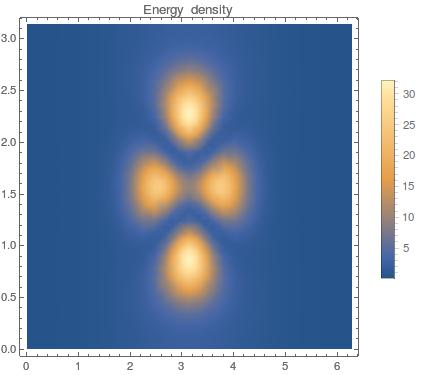
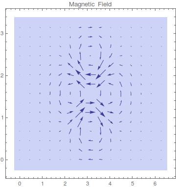
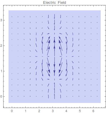
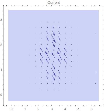
Figure 1: From left to right we can see the energy density $\mathcal{E}$, the magnetic field, the electric field and the current $J_{\mu}$ for a configuration with Baryon charge $B=1$. The electric and magnetic fields vanish at the peaks of the energy density while the current takes its maximum value.

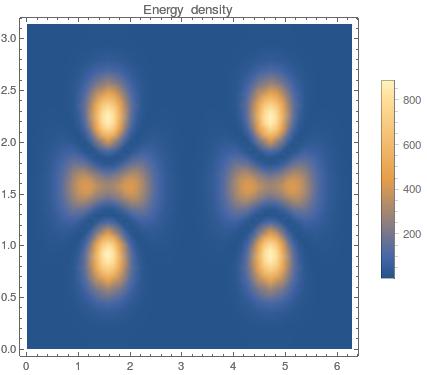
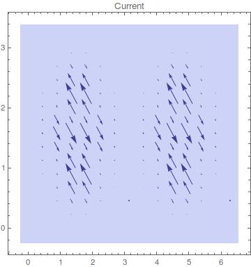
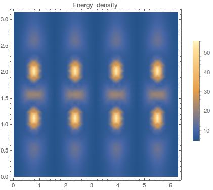
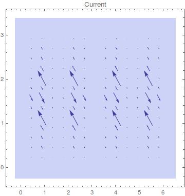
Figure 2: From left to right, crystals of superconducting strings with $B=2$ and $B=4$, respectively. The current is concentrated in the tube-shaped regions defined where (most of) the $\mathcal{E}$ is contained, and vanishes outside the tubes. The maximum values of $\mathcal{E}$ and the current coincide in the lattice, which is periodic in $r$, $\theta$ and perpendicular to the $\phi$ direction, along which the strings exist.

The components of the electric and magnetic fields can be also computed and are given by

$$E_{r}=-\partial_{r}u\ ,\quad E_{\theta}=-\partial_{\theta}u\ ,\quad E_{\phi}=0\ ,$$

$$B_{r}=\frac{1}{L^{3}}\partial_{\theta}u\ ,\quad B_{\theta}=-\frac{1}{L^{3}}\partial_{r}u\ ,\quad B_{\phi}=0\ .$$

3.5 About the existence of exact crystals and the universality of the ansatz

In the previous sections we have shown that the low energy limit of QCD supports the existence of crystals of superconducting Baryonic tubes. Of course, this result is very technical in nature and, a priori, it is not clear whether or not one could have expected the appearance (in the low energy limit of QCD) of topological defects supporting superconducting currents. Here we will give an intuitive argument which justifies why one should have expected the existence of such defects.

The first necessary (but, in general, not sufficient) condition that must be satisfied in order to support the existence of superconductive currents in a relativistic context is the existence of a massless excitation which can be coupled consistently to a U(1) gauge field (see the pioneering paper [27]).

According to Eqs. (13) and (14) the SU(2) valued Skyrme field $U$ describes the dynamical evolution of three scalar degrees of freedom $\alpha$, $\Theta$ and $\Phi$ which are coupled through the non-linear kinetic terms typical of Skyrme like models (see Eq. (50) which is the explicit expression of the Skyrme action in terms of $\alpha$, $\Theta$ and $\Phi$: of course such action is equivalent to the usual one written implicitly in terms of the SU(2) valued field $U$). This fact hides a little bit which is the “best candidate” to carry a superconductive current since our intuition is built on models where the interactions appear in potential terms (like in the Higgs model or in the Ginzburg-Landau model) and not in “generalized kinetic terms” as in the present case. So, the question is: how can we decide a priori which whether or not there is an excitation able to carry a persistent current? In other words, which one of the three degrees of freedom $\alpha$, $\Theta$ and $\Phi$ associated to the SU(2) valued scalar field $U$ can be a carrier of a superconductive current? In what follows we will detail the intuitive arguments that lead us to consider $\Phi$ as the most natural choice.

To illustrate our argument, let us first consider the simpler and well known case of two scalar fields $\Psi^{i}$, with $i=1,2$, interacting with a quartic potential in a SO(2) invariant way,

$$\mathcal{L}=\partial_{\mu}\Psi_{i}\partial^{\mu}\Psi^{i}+\lambda(\Psi_{i}\Psi^{i}-v^{2})^{2}\ .$$ (36)

In order to disclose which degree of freedom is a natural candidate to carry a chiral current, we can write

$$\Psi_{1}=R(x^{\mu})\sin(\chi(x^{\mu}))\ ,\qquad\Psi_{2}=R(x^{\mu})\cos(\chi(x^{\mu}))\ ,$$

then, Eq. (36) becomes

$$\mathcal{L}=\partial_{\mu}R\partial^{\mu}R+R^{2}\partial_{\mu}\chi\partial^{\mu}\chi+\lambda(R^{2}-v^{2})^{2}\ .$$ (37)

From Eq. (37) it is clear that $R$ can not be chiral field because of the presence of a non-trivial potential term that only depends on $R$ and generates a natural mass scale in the dynamics of $R$ (there should be no characteristic mass scale in a superconducting current). On the other hand, $\chi$ (which represents a phase and so is defined only modulo $2\pi$) describes excitations along the valley of the potential, and, consequently, is a more suitable candidate to carry a superconductive current. Of course, all of this is well known in the analysis of the Higgs and Goldstone modes, but this short review helps to identify the correct chiral field in our case in which there is no potential to look at (as the interactions happen in non-linear kinetic-like terms). Moreover, the above Lagrangian can also be naturally coupled to a U(1) gauge field as follows:

$$\mathcal{L}_{\text{U(1)}}=\partial_{\mu}R\partial^{\mu}R+R^{2}\left(\partial_{\mu}\chi-eA_{\mu}\right)\left(\partial^{\mu}\chi-eA^{\mu}\right)+\lambda(R^{2}-v^{2})^{2}-F_{\mu\nu}F^{\mu\nu}.$$ (38)

It is easy to see that the U(1) current $J_{\mu}$ arising from the above action is proportional to $J_{\mu}\sim\left(\partial_{\mu}\chi-eA_{\mu}\right)$. These are part of the main ingredients of [27] to build topological defects supporting superconducting currents. Hence, the fingerprints to identify the degree of freedom (call it for convenience $\Phi^{\ast}$) suitable to carry the superconducting current are, firstly, that such a degree of freedom $\Phi^{\ast}$ should only appear with a kinetic term in the full action of the theory (as $\chi$ in Eq. (37) here above) and without any other explicit non-linear term involving $\Phi^{\ast}$ itself. Secondly, the coupling of the theory with a U(1) gauge theory should only affect the kinetic term of the field $\Phi^{\ast}$. Clearly, the above requirements allow to identify $\chi$ as the field $\Phi^{\ast}$ candidate to be a carrier of a superconducting current in the above example.

What happens in the present case? Obviously, in the Skyrme case there is no interaction potential which is responsible for the interactions term: in all the Skyrme-like models the non-linear behavior is related with generalized kinetic terms. Nevertheless, as can be seen in Eq. (50), the $\alpha$ and $\Theta$ fields have explicit non-linear interaction terms, all of them proportional to $\sin^{2}\alpha$ and/or $\sin^{2}\Theta$. Hence (although in the present case there is no potential which clearly allows to identify the “proper valleys and Goldstone modes”), it is clear that neither $\alpha$ nor $\Theta$ can be the analogue of $\chi$ in the previous example. The reason is that if one sets $\alpha$ to a generic constant value $\Theta$ will still have non-linear interaction terms and viceversa if one sets $\Theta$ to a generic constant value $\alpha$ will still have non-linear interaction terms. Consequently, the fields $\alpha$ and $\Theta$ are rather similar to the field $R$ than to the field $\chi$ in the previous example. The field $\Phi$ on the other hand, has precisely the same characteristics as the field $\chi$ in the previous example: it is only defined modulo $2\pi$ (since $U$ depends on $\Phi$ only through $\sin\Phi$ and $\cos\Phi$) and moreover it appears in the action only with the corresponding kinetic term. Thus, if you set the other fields $\alpha$ and $\Theta$ to generic constant values, then the field $\Phi$ can behave as a chiral massless field. Thus, a priori, one should have expected that also in the (generalized) Skyrme model superconducting Baryonic tubes should be present. Moreover, the minimal coupling of the (generalized) Skyrme model(s) with the Maxwell theory is defined by the following covariant derivative: $\nabla_{\mu}\rightarrow D_{\mu}=\nabla_{\mu}+A_{\mu}[\tau_{3},\cdot]$. From the viewpoint of the $\alpha$, $\Theta$ and $\Phi$ the minimal coupling rule is completely equivalent to change in the action only the derivatives of $\Phi$ as follows $\nabla_{\mu}\Phi\rightarrow D_{\mu}\Phi=\nabla_{\mu}\Phi-2A_{\mu}\Phi$. Hence, also from the viewpoint of the interaction with the Maxwell theory, the field $\Phi$ is the analogue of $\chi$ in the previous example and this is exactly what we need, according to Witten [14], to have a superconducting current.

As a last remark, at a first glance, one could also argue that the presence of a mass term for the Pions should destroy superconductivity. In fact, this is not the case since, in terms of $\alpha$, $\Theta$ and $\Phi$, the mass term for the Pions is $m_{\pi}^{2}(1-\cos\alpha)$, and it only affects $\alpha$ (in the same way as a mass term in the previous example would only affect $R$ but would not set a mass scale for $\chi$).

These are the intuitive arguments which strongly suggest a priori that it certainly pay off to look for superconducting solitons in the generalized Skyrme model(s) and that $\Phi$ should be the superconducting carrier.

Furthermore, by requiring that $\nabla_{\mu}\Phi\nabla^{\mu}\Phi$ vanishes (as it is expected for chiral fields), the field equations are enormously simplified (see Eqs. (51), (52) and (53) on Appendix II). This simplification occurs not only on the Skyrme model case, but even if higher derivative order terms are considered, as we have already discussed.

3.6 Stability analysis

One of the most intriguing results of the present framework is that the physical properties of these superconducting Baryonic tubes remain the same no matter how many subleading terms are included in the generalized Skyrme model. In other words, these topologically non-trivial configurations are almost “theory independent”. As it has been already emphasized, this happens since the ansatz defined in Eq. (17) works in exactly the same way without any change at all no matter how many higher order terms are included in the generalized Skyrme action. In particular, the field equations will always be reduced to a single integrable ODE for $\alpha$ and the corresponding configurations will describe superconducting tubes. Hence, the present topological gauged solitons are likely to be a universal feature of QCD as they stay the same at any order in the large N expansion.

To give a flavor of why such a property is so surprising, let us consider the ’t Hooft-Polyakov monopole [39], [40]. The stability of these configurations in the Georgi-Glashow model is of course very well understood. However, if one deforms even slightly the theory, the properties of the ’t Hooft-Polyakov monopole are going to change as well (see, for instance, [41] and references therein). To give just an example: in [41] the authors considered a very natural correction to the Georgi-Glashow model which leads to a non-spherical deformation of the ’t Hooft-Polyakov monopole (so that, in particular, the ansatz for the ’t Hooft-Polyakov monopole must be changed accordingly). Consequently, the shape of non-Abelian monopoles is also going to change when these types of deformations of the Yang-Mills theory are included. On the other hand, the superconducting Baryonic tubes constructed here keep their properties at any order in the large N expansion. To the best of authors knowledge, these are the first examples of “universal” gauged solitons in the low energy limit of QCD described by an ansatz able to survive to all the subleading large N corrections. Indeed, the subleading corrections to the generalized Skyrme model will only change slightly the plot of $\alpha(r)$ keeping unchanged the plots and the properties of the superconducting currents and of the energy density (see Figure 3). Here below we write the field equation for $\alpha(r)$ with corrections up to order $\mathcal{L}_{12}$ together with the plots of the energy density of the superconducting tubes in the sector with Baryonic charge $B=1$ in Figure 4. For this we have chosen $K=2$, $\lambda=1$, $c_{6}=c_{8}=c_{12}=\frac{1}{5}$, $m=0$ and $q=p=1$.

The field equations are given by

$$\alpha^{\prime\prime}-\frac{q^{2}}{2}\sin(2\alpha)+\frac{4m^{2}L^{2}}{K}\sin{\alpha}+\frac{\lambda q^{2}}{L^{2}}\sin(\alpha)[\cos(\alpha)\alpha^{\prime 2}+\sin(\alpha)\alpha^{\prime\prime}]$$

$$-\frac{3c_{8}q^{4}}{KL^{6}}\sin^{3}(\alpha)[\cos(\alpha)\alpha^{\prime 2}+\sin(\alpha)\alpha^{\prime\prime}]\alpha^{\prime 2}-\frac{15c_{12}q^{6}}{KL^{6}}\sin^{5}(\alpha)[\cos(\alpha)\alpha^{\prime 2}+\sin(\alpha)\alpha^{\prime\prime}]\alpha^{\prime 4}\ =\ 0\ ,$$ (39)

that can be written again as a first order equation

$$\left\{X\left(\alpha\right)\left(\alpha^{\prime}\right)^{2}+Z\left(\alpha\right)+\tilde{E}_{0}\right\}^{\prime}=0\ ,$$ (40)

where in this case

$$X\left(\alpha\right)=1+\frac{\lambda q^{2}}{L^{2}}\sin^{2}(\alpha)-\frac{3c_{8}q^{4}}{2KL^{6}}\sin^{4}(\alpha)\alpha^{\prime 2}-\frac{5c_{12}q^{6}}{KL^{10}}\sin^{6}\alpha(\alpha^{\prime})^{4}\ ,$$

$$Z(\alpha)=\frac{q^{2}}{2}\cos(2\alpha)-\frac{8m^{2}L^{2}}{K}\cos(\alpha)\ .$$

Note also that Eq. (40) can be seen as a cubic polynomial in the variable $z=\alpha^{\prime 2}$ which allows, once again, to reduce the complete field equations to a simple quadrature of the form:

$$\frac{d\alpha}{\widetilde{\chi}^{1/2}}=\pm dr\ ,\qquad\widetilde{\chi}=\widetilde{\chi}(\alpha,E_{0})\ ,$$

where $\widetilde{\chi}(\alpha,E_{0})$ is the positive real root of the cubic polynomial in $z=\alpha^{\prime 2}$ defined in Eq. (40). The integration constant $\tilde{E}_{0}$ always allows such polynomial to have positive real roots.

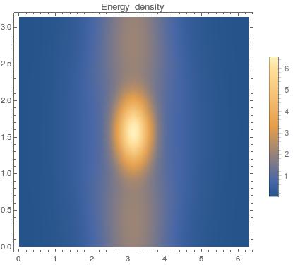
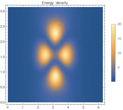
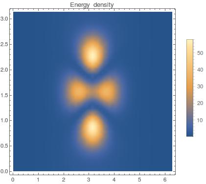
Figure 3: Energy density for different configurations with $B=1$. From left to right: energy density only including the non-linear sigma model contribution, then up to the Skyrme contribution, up to $\mathcal{L}_{6}$, up to $\mathcal{L}_{8}$ and finally up to order $\mathcal{L}_{12}$ .

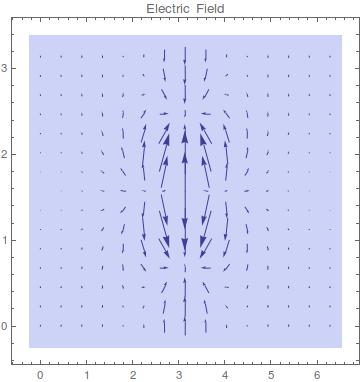
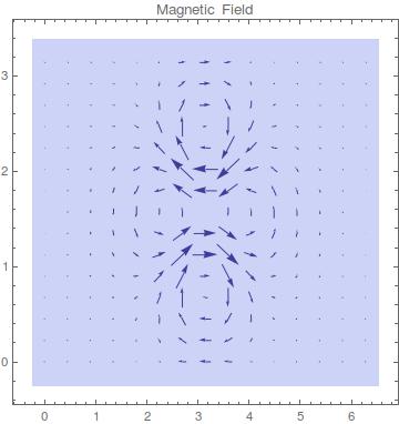
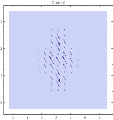
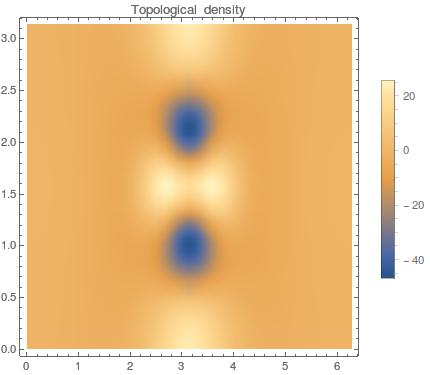
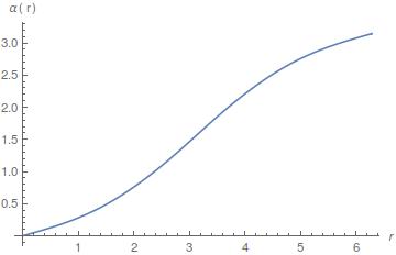
Figure 4: From left to right: Energy density $\mathcal{E}$, electric field, magnetic field, current, topological density $\rho_{\text{B}}$ and radial profile $\alpha(r)$, up to the contribution $\mathcal{L}_{12}$ for the configuration with $B=1$.

3.6.1 Perturbations on the profile

A remark on the stability of the above superconductive tubes is in order. In many situations, when the hedgehog property holds (so that the field equations reduce to a single equation for the profile) the most dangerous perturbations are perturbations of the profile which keep the structure of the hedgehog ansatz (see [42], [43] and references therein). In the present case these are perturbations of the following type:

$$\alpha\rightarrow\alpha+\varepsilon\xi\left(r\right)\ ,\ \ \ 0<\varepsilon\ll 1\ ,$$ (41)

which do not change the Isospin degrees of freedom associated with the functions $\Theta$ and $\Phi$. A direct computation reveals that the linearized version of Eq. (19) around a background solution $\alpha_{0}\left(r\right)$ of Baryonic charge $B=np$ always has the following zero-mode: $\xi\left(r\right)=\nabla_{r}\alpha_{0}\left(r\right)$. Due to the fact that the integration constant $E_{0}$ (defined in Eqs. (20), (21) and (22)) can always be chosen in such a way that $\nabla_{r}\alpha_{0}\left(r\right)$ never vanishes, the zero mode $\xi\left(r\right)$ has no node so that it must be the perturbation with lowest energy. Thus, the present solutions are stable under the above potentially dangerous perturbations. Although this is not a complete proof of stability, it is a very non-trivial test.

3.6.2 Electromagnetic perturbations

A very useful approach to study the stability of the superconducting Baryonic tubes is to perform electromagnetic perturbations on the effective medium defined by the topological solitons. This is a good approach in the ’t Hooft limit, since in the semiclassical interaction Photon-Baryon, the Baryon is essentially unaffected due to the Photon has zero mass (see [44]).

The complete stability analysis requires to study the most general perturbations of the solutions defined in Eqs. (17), (21) and (22). This is a very hard task even numerically as it involves a coupled system of linear PDEs, therefore in practical terms, consider only electromagnetic perturbations greatly simplifies the stability analysis and allows to reveal very relevant features of the superconducting tubes, as we will see immediately.

Here we will analyze the simplest non-trivial case which is related to the role of the subleading corrections in the ’t Hooft expansion to the Skyrme model of the sixth order. As it has been already emphasized in the previous sections such sixth order term does not even appear in the equation for the profile (while it does enter in the corresponding Maxwell equations). This is very interesting since it shows that, despite the universal character of the present crystals of gauged solitons (which are almost unaffected by the subleading terms), their stability properties may depend explicitly on the subleading terms themselves. Also for simplicity reasons, we will set $m$ to zero.

Let us consider the following perturbations on the Maxwell potential

$$(u,0,0,-Lu)\rightarrow(u+\varepsilon\xi_{1},0,0,-Lu+\varepsilon\xi_{2})\ ,\qquad\xi_{i}=\xi_{i}(t,r,\theta,\phi)\ ,\qquad 0<\varepsilon\ll 1\ .$$

At first order in the parameter $\varepsilon$ the Maxwell equations become

$$\partial_{\theta}(\partial_{\phi}\xi_{2}-L^{2}\partial_{t}\xi_{1})=0\ ,$$

$$\partial_{r}(\partial_{\phi}\xi_{2}-L^{2}\partial_{t}\xi_{1})=0\ ,$$

$$(\partial_{r}^{2}+\partial_{\theta}^{2}+\partial_{\phi}^{2})\xi_{1}-\partial_{\phi}\partial_{t}\xi_{2}+V\xi_{1}\ =\ 0\ ,$$

$$(\partial_{r}^{2}+\partial_{\theta}^{2}-L^{2}\partial_{t}^{2})\xi_{2}+L^{2}\partial_{\phi}\partial_{t}\xi_{1}+V\xi_{2}\ =\ 0\ ,$$

where $V$ and $\Omega(\alpha)$ are defined in Eqs. (29) and (31) (up to sixth order). Note that, since we want to test linear stability one should check the (absence of) growing modes in time. This implies that $\xi_{1}$ and $\xi_{2}$ must depend on the temporal coordinate. But, according to the previous equations if $\xi_{1}$ and $\xi_{2}$ depend on time these functions must also depend on the coordinate $\phi$, that is

$$\partial_{t}\xi_{i}\neq 0\ ,\qquad\partial_{\phi}\xi_{i}\neq 0\ ,\qquad\xi_{i}=\{\xi_{1},\xi_{2}\}\ .$$

We can assume that

$$\partial_{\phi}\xi_{2}=L^{2}\partial_{t}\xi_{1}\ .$$

By consider the Fourier transformation in the coordinate $\phi$ we get an equation for $\widehat{\xi}_{i}$ in the form

$$-\Box\widehat{\xi}_{i}+(k^{2}-V)\widehat{\xi}_{i}=0\ ,\qquad\Box\equiv-L^{2}\partial_{t}^{2}+\partial_{r}^{2}+\partial_{\theta}^{2}\ ,$$

where

$$\widehat{\xi}_{i}(t,r,\theta,k)=\int\xi_{i}(t,r,\theta,\phi)e^{-ik\phi}d\phi\ ,$$

is the Fourier transform of $c_{i}$, and the non-vanishing eigenvalue $k=l/(2\pi)$ is the wave-number along the $\phi$-direction, with $l$ a non-vanishing integer.

According to Duhamel’s principle (see, for instance, [45] and references therein), an inhomogeneous equation for a function $W=W(x,t)$ of the form

$$(d_{t}^{2}+M)W=f\ ,$$

with $M$ a non-negative operator and initial conditions $W(\cdot,0)=\psi_{1}$, $\partial_{t}W(\cdot,0)=\psi_{2}$, has the following general solution

$$W(\cdot,t)=\partial_{t}B(t)\psi_{1}+B(t)\psi_{2}+\int_{0}^{t}B(t-\tau)f(\tau)d\tau\ ,\quad B(t)=M^{-\frac{1}{2}}\sin(tM^{\frac{1}{2}})\ .$$

In our case, to ensure that the perturbed Maxwell equation can be solved we need to demand that $V_{\text{eff}}>0$, with

$$V_{\text{eff}}=k^{2}-V\ .$$ (42)

Since $V$ depends on $\alpha$ and the square of its derivative $\alpha^{\prime}=\alpha^{\prime}(E_{0})$, defined via Eq. (20), one can find the following upper bound to the potential $V$:

$$\left|V\right|\leq V_{\text{max}}<\frac{4}{L^{2}}\biggl{(}KL^{4}+(q^{2}+E_{0})\lambda KL^{2}+2q^{2}c_{6}E_{0}\biggl{)}\ .$$

Then, a necessary condition for a positive defined effective potential $V_{\text{eff}}$ in Eq. (42) is

$$\left(\frac{l}{2\pi}\right)^{2}-\frac{4}{x}\biggl{(}Kx^{2}+(q^{2}+E_{0})\lambda Kx+2q^{2}c_{6}E_{0}\biggl{)}\geq 0\ ,$$ (43)

$$x=L^{2}\ ,$$

(the most restrictive case being the one with $l^{2}=1$ as it is easier to satisfy the above inequality when $l^{2}$ is large). The above inequality set an upper bound on the allowed values of $L$ (which is the same as a lower bound on the allowed values of Baryon densities):

$$\frac{x}{16\pi^{2}}-\biggl{(}Kx^{2}+(q^{2}+E_{0})\lambda Kx+2q^{2}c_{6}E_{0}\biggl{)}\geq 0\ .$$ (44)

The above inequality is equivalent to

$$L_{\text{Min}}^{2}\leq x\leq L_{\text{Max}}^{2}\ ,$$ (45)

$$L_{\text{Max}}^{2} = \frac{1}{2K}\biggl{(}\frac{1}{16\pi^{2}}-(E_{0}+q^{2})K\lambda+\sqrt{\biggl{(}\frac{1}{16\pi^{2}}-(E_{0}+q^{2})K\lambda\biggl{)}^{2}-8c_{6}q^{2}E_{0}K}\biggl{)}\ ,$$ (46)

$$L_{\text{Min}}^{2} = \frac{1}{2K}\biggl{(}\frac{1}{16\pi^{2}}-(E_{0}+q^{2})K\lambda-\sqrt{\biggl{(}\frac{1}{16\pi^{2}}-(E_{0}+q^{2})K\lambda\biggl{)}^{2}-8c_{6}q^{2}E_{0}K}\biggl{)}\ ,$$ (47)

together with the obvious condition that

$$x\geq 0\ .$$ (48)

Thus, in the range of parameters in which $L_{\text{Max}}^{2}$ is positive (which always exists) the conditions on $L^{2}$ is

$$L^{2}<\frac{1}{2K}\biggl{(}\frac{1}{16\pi^{2}}-(E_{0}+q^{2})K\lambda+\sqrt{\biggl{(}\frac{1}{16\pi^{2}}-(E_{0}+q^{2})K\lambda\biggl{)}^{2}-8c_{6}q^{2}E_{0}K}\biggl{)}\ .$$

Thus, at a first glance, from Eq. (19) one could think that the presence of the $c_{6}$, which for energetic considerations must be positive (see Eq. (34)), do not play any role in the perturbation of the system. However, it is quite interesting to see that this term can in fact affect the stability of the system determining the maximum allowed value of the size of the box in which the superconducting strings are confined. We hope to come back on the physical properties of these gauged crystals in the low energy limit of QCD in a future publication.

4 Conclusions and perspectives

The Maxwell-gauged Skyrme model in $(3+1)$-dimensions together with all the subleading corrections in the ’t Hooft expansion admit configurations describing ordered arrays of Baryonic superconducting tubes where (most of) the Baryonic charge and total energy is concentrated in tube-shaped regions. The corresponding current cannot be deformed continuously to zero as it is tied to the topological charge. Quite remarkably, no matter how many subleading terms are included, these ordered arrays of gauged solitons are described by the very same ansatz and keep their main properties manifesting a sort of universal character. The similarity with the plots obtained numerically in the analysis of nuclear spaghetti phase is quite amusing [9]. These results open the unprecedented possibility to analyze these complex structures with analytic tools which are able to disclose novel features which are difficult to analyze with many body simulations. On the other hand, the subleading terms in the ’t Hooft expansion (which almost do not affect the solutions of the field equations) do, in fact, affect the stability properties of the superconducting tubes setting upper bounds on the allowed values of the spatial volume in which they can live.

Acknowledgments

F. C. has been funded by Fondecyt Grants 1200022. M. L. and A. V. are funded by FONDECYT post-doctoral grant 3190873 and 3200884. The Centro de Estudios Científicos (CECs) is funded by the Chilean Government through the Centers of Excellence Base Financing Program of Conicyt.

Appendix I: Explicit tensors

From the ansatz defined in Eqs. (12), (13), (14), (17) and (27), the explicit expression of the matrix $U$, the components of the tensor $L_{\mu}$ and the components of the current $J_{\mu}$ are given by

$$U=\begin{pmatrix}\cos(\alpha)+i\sin(\alpha)\cos(q\theta)&ie^{-ip(t/L-\phi)}\sin(\alpha)\sin(q\theta)\\ ie^{ip(t/L-\phi)}\sin(\alpha)\sin(q\theta)&\cos(\alpha)-i\sin(\alpha)\cos(q\theta)\end{pmatrix}\ ,$$

$$L_{t}=(\frac{p}{L}-2u)\begin{pmatrix}i\sin^{2}\alpha\sin^{2}(q\theta)&e^{-ip(t/L-\phi)}\sin\alpha\sin(q\theta)(\cos\alpha-i\sin\alpha\cos(q\theta)\\ -e^{ip(t/L-\phi)}\sin\alpha\sin(q\theta)(\cos\alpha+i\sin\alpha\cos(q\theta)&-i\sin^{2}\alpha\sin^{2}(q\theta)\end{pmatrix}\ ,$$

$$L_{r}=\begin{pmatrix}i\cos(q\theta)\alpha^{\prime}&e^{-ip(t/L-\phi)}\sin(q\theta)\alpha^{\prime}\\ ie^{ip(t/L-\phi)}\sin(q\theta)\alpha^{\prime}&-i\cos(q\theta)\alpha^{\prime}\end{pmatrix}\ ,$$

$$L_{\theta}=\begin{pmatrix}-iq\sin\alpha\cos\alpha\sin(q\theta)&qe^{-ip(t/L-\phi)}\sin\alpha(\sin\alpha+i\cos\alpha\cos(q\theta))\\ -qe^{ip(t/L-\phi)}\sin\alpha(\sin\alpha-i\cos\alpha\cos(q\theta))&iq\sin\alpha\cos\alpha\sin(q\theta)\end{pmatrix}\ ,$$

$$L_{\phi}=-LL_{t}\ ,$$

$$J_{t}=\frac{2}{L^{4}}\sin^{2}(\alpha)\sin^{2}(q\theta)\biggl{(}KL^{2}(L^{2}+q^{2}\lambda\sin^{2}(\alpha)+\lambda\alpha^{\prime 2})+q^{2}\sin^{2}(\alpha)\alpha^{\prime 2}\biggl{[}2c_{6}+\frac{c_{8}}{L^{2}}(q^{2}\sin^{2}(\alpha)+\alpha^{\prime 2})\biggl{]}\biggl{)}$$

$$\times\biggl{(}\frac{p}{L}-2u\biggl{)}\ ,$$

$$J_{r}=J_{\theta}=0\ ,\quad J_{\phi}=-LJ_{t}\ .$$

Appendix II: Reducing the Skyrme equations

In this appendix we will show how and why the Skyrme equations (using the ansatz defined by Eqs. (12), (13), (14), and (17)) are reduced to just one integrable ODE for the soliton profile $\alpha=\alpha(r)$. To see this fact it is possible to take two paths, as we detail below.

In order to make this reduction clear, in this appendix we will consider the action in Eq. (1) without the higher order terms and without the coupling with Maxwell theory, i.e. we will deal only with the usual Skyrme action

$$I_{\text{Skyrme}}=\int\frac{d^{4}v}{4}\left[K\mathrm{Tr}\left(L^{\mu}L_{\mu}+\frac{\lambda}{8}G_{\mu\nu}G^{\mu\nu}\right)\right]\ ,$$ (49)

$$L_{\mu}=U^{-1}\nabla_{\mu}U\ ,\quad G_{\mu\nu}=[L_{\mu},L_{\nu}]\ ,\quad d^{4}v=d^{4}x\sqrt{-g}\ ,$$

$$U\in\text{SU(2)}\ ,\ \ L_{\mu}=L_{\mu}^{j}t_{j}\ ,\ \ t_{j}=i\sigma_{j}\ .$$

The reason for doing this is that the mechanism which makes the present strategy successful with the usual Skyrme model works in exactly the same way when the higher order terms are included.

The most direct way to see that the Skyrme equations are reduced to just one equation with the ansatz defined by Eqs. (12), (13), (14), and (17) corresponds to write the action in Eq. (49) explicitly in terms of the functions $\alpha=\alpha(x^{\mu})$, $\Theta=\Theta(x^{\mu})$ and $\Phi=\Phi(x^{\mu})$, according to Eqs. (13), (14). In this parameterization Eq. (49) becomes

$$I_{\text{Skyrme}}=\frac{K}{2}\int d^{4}v\left(\begin{array}[]{c}\nabla_{\mu}\alpha\nabla^{\mu}\alpha+\sin^{2}{\alpha}\nabla_{\mu}\Theta\nabla^{\mu}\Theta+\sin^{2}{\alpha}\sin^{2}{\Theta}\nabla_{\mu}\Phi\nabla^{\mu}\Phi\\ +\lambda\left(\begin{array}[]{c}\sin^{2}{\alpha}\left((\nabla_{\mu}\alpha\nabla^{\mu}\alpha)(\nabla_{\nu}\Theta\nabla^{\nu}\Theta)-(\nabla_{\mu}\alpha\nabla^{\mu}\Theta)^{2}\right)\\ +\sin^{2}{\alpha}\sin^{2}{\Theta}\left((\nabla_{\mu}\alpha\nabla^{\mu}\alpha)(\nabla_{\nu}\Phi\nabla^{\nu}\Phi)-(\nabla_{\mu}\alpha\nabla^{\mu}\Phi)^{2}\right)\\ +\sin^{4}{\alpha}\sin^{2}{\Theta}\left((\nabla_{\mu}\Theta\nabla^{\mu}\Theta)(\nabla_{\nu}\Phi\nabla^{\nu}\Phi)-(\nabla_{\mu}\Theta\nabla^{\mu}\Phi)^{2}\right)\end{array}\right)\end{array}\right)\ .$$ (50)

Now, varying the action in Eq. (50) w.r.t the functions $\alpha$, $\Theta$, $\Phi$, in a long but direct calculation, we get to the following set of equations:

$$\begin{array}[]{c}\left(-\Box\alpha+\sin(\alpha)\cos(\alpha)\left(\nabla_{\mu}\Theta\nabla^{\mu}\Theta+\sin^{2}\Theta\nabla_{\mu}\Phi\nabla^{\mu}\Phi\right)\right)\\ +\lambda\left(\begin{array}[]{c}\sin(\alpha)\cos(\alpha)\left((\nabla_{\mu}\alpha\nabla^{\mu}\alpha)(\nabla_{\nu}\Theta\nabla^{\nu}\Theta)-(\nabla_{\mu}\alpha\nabla^{\mu}\Theta)^{2}\right)\\ +\sin(\alpha)\cos(\alpha)\sin^{2}(\Theta)\left((\nabla_{\mu}\alpha\nabla^{\mu}\alpha)(\nabla_{\nu}\Phi\nabla^{\nu}\Phi)-(\nabla_{\mu}\alpha\nabla^{\mu}\Phi)^{2}\right)\\ +2\sin^{3}(\alpha)\cos(\alpha)\sin^{2}(\Theta)\left((\nabla_{\mu}\Theta\nabla^{\mu}\Theta)(\nabla_{\nu}\Phi\nabla^{\nu}\Phi)-(\nabla_{\mu}\Theta\nabla^{\mu}\Phi)^{2}\right)\\ -\nabla_{\mu}\left(\sin^{2}(\alpha)(\nabla_{\nu}\Theta\nabla^{\nu}\Theta)\nabla^{\mu}\alpha\right)+\nabla_{\mu}\left(\sin^{2}(\alpha)(\nabla_{\nu}\alpha\nabla^{\nu}\Theta)\nabla^{\mu}\Theta\right)\\ -\nabla_{\mu}\left(\sin^{2}(\alpha)\sin^{2}(\Theta)(\nabla_{\nu}\Phi\nabla^{\nu}\Phi)\nabla^{\mu}\alpha\right)+\nabla_{\mu}\left(\sin^{2}(\alpha)\sin^{2}(\Theta)(\nabla_{\nu}\alpha\nabla^{\nu}\Phi)\nabla^{\mu}\Phi\right)\end{array}\right)\end{array}=0\ ,$$ (51)

$$\begin{array}[]{c}\left(-\sin^{2}(\alpha)\Box\Theta-2\sin(\alpha)\cos(\alpha)\nabla_{\mu}\alpha\nabla^{\mu}\Theta+\sin^{2}(\alpha)\sin(\Theta)\cos(\Theta)\nabla_{\mu}\Phi\nabla^{\mu}\Phi\right)\\ +\lambda\left(\begin{array}[]{c}\sin^{2}(\alpha)\sin(\Theta)\cos(\Theta)\left((\nabla_{\mu}\alpha\nabla^{\mu}\alpha)(\nabla_{\nu}\Phi\nabla^{\nu}\Phi)-(\nabla_{\mu}\alpha\nabla^{\mu}\Phi)^{2}\right)\\ +\sin^{4}(\alpha)\sin(\Theta)\cos(\Theta)\left((\nabla_{\mu}\Theta\nabla^{\mu}\Theta)(\nabla_{\nu}\Phi\nabla^{\nu}\Phi)-(\nabla_{\mu}\Theta\nabla^{\mu}\Phi)^{2}\right)\\ -\nabla_{\mu}\left(\sin^{2}(\alpha)(\nabla_{\nu}\alpha\nabla^{\nu}\alpha)\nabla^{\mu}\Theta\right)+\nabla_{\mu}\left(\sin^{2}(\alpha)(\nabla_{\nu}\alpha\nabla^{\nu}\Theta)\nabla^{\mu}\alpha\right)\\ -\nabla_{\mu}\left(\sin^{4}(\alpha)\sin^{2}(\Theta)(\nabla_{\nu}\Phi\nabla^{\nu}\Phi)\nabla^{\mu}\Theta\right)+\nabla_{\mu}\left(\sin^{4}(\alpha)\sin^{2}(\Theta)(\nabla_{\nu}\Theta\nabla^{\nu}\Phi)\nabla^{\mu}\Phi\right)\end{array}\right)\end{array}=0\ ,$$ (52)

$$\begin{array}[]{c}\left(-\sin^{2}(\alpha)\sin^{2}(\Theta)\Box\Phi-2\sin(\alpha)\cos(\alpha)\sin^{2}(\Theta)\nabla_{\mu}\alpha\nabla^{\mu}\Phi-2\sin^{2}(\alpha)\sin(\Theta)\cos(\Theta)\nabla_{\mu}\Theta\nabla^{\mu}{\Phi}\right)\\ +\lambda\left(\begin{array}[]{c}-\nabla_{\mu}\left[\sin^{2}(\alpha)\sin^{2}(\Theta)(\nabla_{\nu}\alpha\nabla^{\nu}\alpha)\nabla^{\mu}\Phi\right]+\nabla_{\mu}\left[\sin^{2}(\alpha)\sin^{2}(\Theta)(\nabla_{\nu}\alpha\nabla^{\nu}\Phi)\nabla^{\mu}\alpha\right]\\ -\nabla_{\mu}\left[\sin^{4}(\alpha)\sin^{2}(\Theta)(\nabla_{\nu}\Theta\nabla^{\nu}\Theta)\nabla^{\mu}\Phi\right]+\nabla_{\mu}\left[\sin^{4}(\alpha)\sin^{2}(\Theta)(\nabla_{\nu}\Theta\nabla^{\nu}\Phi)\nabla^{\mu}\Theta\right]\end{array}\right)\end{array}=0\ .$$ (53)

The equations system written above are completely equivalent to the system in Eq. (5) when the parameterization in Eqs. (13) and (14) is considered. For instance, one can check that with this parametrization the original spherical hedgehog ansatz of Skyrme himself [13] reads

$$\alpha=\alpha(x)\ ,\quad\Theta=\theta\ ,\quad\Phi=\phi\ ,$$ (54)

$$ds^{2}=-dt^{2}+dx^{2}+x^{2}\left(d\theta^{2}+\sin^{2}\theta d\phi^{2}\right)\ ,$$ (55)

where $x$ is the radial coordinate of flat space-time metric in spherical coordinates. If one plugs the ansatz in Eqs. (54) and (55) into the field equations (51), (52) and (53) one can see that, first of all, the field equations for $\Theta$ and $\Phi$ are identically satisfied and, secondly, that the remaining field equation for $\alpha$ reduces to the well known equation for the profile of the spherical Skyrmion. This is the defining characteristic of the hedgehog ansatz and is equivalent to the statement that the field equations reduce consistently to just one ODE for the profile $\alpha$.

At this point we can directly evaluate the ansatz in Eq. (17) into Eqs. (51), (52) and (53) and check whether or not the same hedgehog property holds. One could think that the spherical symmetry is relevant to get a good hedgehog ansatz but the present analysis show that the hedgehog property does not need spherical symmetry at all. Considering that our ansatz satisfies the useful relations in Eqs. (16) and (18), namely

$$\nabla_{\mu}\Phi\nabla^{\mu}\alpha=\nabla_{\mu}\alpha\nabla^{\mu}\Theta=\nabla_{\mu}\Phi\nabla^{\mu}\Phi=\nabla_{\mu}\Theta\nabla^{\mu}\Phi=\Box\Theta=\Box\Phi=0\ ,$$

one can see that Eqs. (52) and (53) are identically satisfied, while Eq. (51) leads to

$$-\Box\alpha+\sin(\alpha)\cos(\alpha)\nabla_{\mu}\Theta\nabla^{\mu}\Theta+\lambda\sin(\alpha)\cos(\alpha)\nabla_{\mu}\alpha\nabla^{\mu}\alpha\nabla_{\nu}\Theta\nabla^{\nu}\Theta=0\ .$$ (56)

Eq. (56) is an integrable ODE for the soliton profile $\alpha$. In fact, taking into account that

$$\Box\alpha=\frac{1}{L^{2}}\alpha^{\prime\prime}\ ,\quad\nabla_{\mu}\Theta\nabla^{\mu}\Theta=\frac{q^{2}}{L^{2}}\ ,\quad\nabla_{\mu}\alpha\nabla^{\mu}\alpha=\frac{1}{L^{2}}\alpha^{\prime 2}\ ,$$

the above equation becomes

$$\alpha^{\prime\prime}-\frac{q^{2}}{2}\sin(2\alpha)-\frac{\lambda q^{2}}{2L^{2}}\sin(2\alpha)\alpha^{\prime 2}\ =\ 0\ .$$

Note also that using

$$\sin(2\alpha)\alpha^{\prime 2}=[\sin^{2}(\alpha)\alpha^{\prime}]^{\prime 2}(\alpha)-\sin^{2}(\alpha)\alpha^{\prime\prime}\ ,$$

we finally arrive to the following equation for $\alpha$:

$$\alpha^{\prime\prime}-\frac{q^{2}}{2}\sin(2\alpha)+\frac{\lambda q^{2}}{L^{2}}\sin(\alpha)[\cos(\alpha)\alpha^{\prime 2}+\sin(\alpha)\alpha^{\prime\prime}]\ =\ 0\ ,$$

which, of course, coincides with Eq. (19).

On the other hand, one could be dissatisfied with the above method to establish the hedgehog property since in most textbook such a property is defined by looking at the SU(2) valued field without using the explicit  parametrization in terms of the fields $\alpha$, $\Theta$ and $\Phi$. Here we offer another method to derive the hedgehog property which perhaps is more familiar to many of the readers. This method uses the properties of the normalized Isospin vector $n_{i}$ of the generalized hedgehog ansatz in Eq. (51), (52) and (53), is using.

Let us remind that the most general parametrization for the Skyrme field is

$$U=Y^{0}\mathbb{I}+Y^{i}t_{i}\ ,\quad(Y^{0})^{2}+Y_{i}Y^{i}=1\ ,$$

$$Y^{0}=\cos(\alpha)\ ,\quad Y^{i}=\sin(\alpha)n^{i}\ ,\quad n_{i}n^{i}=1\ ,$$

$$n^{1}=\cos\Theta\sin\Phi\ ,\quad n^{2}=\sin\Theta\sin\Phi\ ,\quad n^{3}=\cos\Theta\ ,$$

and the Maurer-Cartan form reads

$$L_{\mu}=U^{-1}\nabla_{\mu}U=L_{\mu}^{i}t_{i}\ ,\quad t_{i}=i\sigma_{i}\ ,$$

where the generators of the SU(2) group, $t_{i}$, satisfy

$$[t_{i},t_{j}]=-2\epsilon_{ijk}t^{k}\ ,\qquad t_{i}t_{j}=-\delta_{ij}\mathbb{I}-\epsilon_{ijk}t^{k}\ .$$

One can check that, for the ansatz in Eq. (17), the $n_{i}$ vectors satisfy the following eigenvalue equation

$$\Box n^{i}\ =\ \Sigma n^{i}\ ,\qquad\Sigma=-\frac{q^{2}}{L^{2}}\ .$$ (57)

It is worth to note that the original ansatz for the spherical Skyrmion in Eqs. (54) and (55) satisfies a similar property (but with a different $\Sigma$ which depends explicitly on the radial coordinate: thus, we can say that in this sense the present generalized hedgehog ansatz is simpler than the usual spherical hedgehog ansatz). Eq. (57) is a very important result since it allows to reduced all the Skyrme system to just only one equation for the soliton profile thanks to a very nice factorization property of the complete field equations (such a factorization is the matrix version of-and completely equivalent to-the property discussed above which is responsible for the fact that the three Skyrme field equations (51), (52) and (53) for $\alpha$, $\Theta$ and $\Phi$ reduce to just one equation for $\alpha$).

One can directly check that the components of the Maurer-Cartan tensor $L_{\mu}$ defined above are

$$L_{\mu}^{k}\ =\ Y^{0}\nabla_{\mu}Y^{k}-Y^{k}\nabla_{\mu}Y^{0}+\epsilon^{ijk}Y_{i}\nabla_{\mu}Y_{j}$$

$$\ =\ n^{k}\nabla_{\mu}\alpha+\frac{1}{2}\sin(2\alpha)\nabla_{\mu}n^{k}+\epsilon^{ijk}\sin^{2}(\alpha)n_{i}\nabla_{\mu}n_{j}\ .$$ (58)

Now, according to Eq. (5), the Skyrme equations have the following general form

$$\nabla^{\mu}\left(L_{\mu}+\frac{\lambda}{4}[L^{\nu},G_{\mu\nu}]\right)=0\ .$$ (59)

Using Eqs. (57), (58) and

$$\nabla_{\mu}n^{i}\nabla^{\mu}\alpha=0\ ,\quad n_{i}\nabla_{\mu}n^{i}=0\ ,\quad\nabla^{\mu}n_{i}\nabla_{\mu}n^{i}=-\Sigma\ ,$$

we can compute both terms in the Skyrme equation separately. For the first term we have

$$\nabla^{\mu}L_{\mu}^{k}=n^{k}\left(\Box\alpha+\frac{1}{2}\Sigma\sin(2\alpha)\right)\ .$$ (60)

Hence, one can see that the divergence $\nabla^{\mu}L_{\mu}^{k}$ of the $L_{\mu}^{k}$ tensor in Eq. (60) (that corresponds to the NLSM field equations) is factorized into the Isospin vector $n^{k}$ itself (which obviously never vanishes) time a factor which depends on $\alpha$. Consequently, in the NLSM case, such a factor is nothing but the equation for the profile $\alpha$. Hence, the choice of $\alpha$ and of the Isospin vector $n^{k}$ in Eq. (51), (52) and (53) reduces the three field equations of the NLSM

$$\nabla^{\mu}L_{\mu}^{k}=0$$

to just

$$\Box\alpha+\frac{1}{2}\Sigma\sin(2\alpha)=0\ .$$

The factorization of the divergence $\nabla^{\mu}L_{\mu}^{k}$ of the $L_{\mu}^{k}$ tensor in Eq. (60) is the matrix form of the property stated here above that the field equations (51), (52) and (53) reduce to just one equation for the soliton profile $\alpha$: however, this “matrix form” of the hedgehog property can be more familiar to most of the readers so that, for pedagogical reasons we have included it here in the present discussion. Once again, we see that the hedgehog property is not related at all with the spherical symmetry and nice ansatz can be constructed even at finite density and without spherical symmetry. Even more, the present non-spherical hedgehog, useful to describe multi-solitonic solutions at finite Baryon density is actually simpler than the spherical hedgehog (which describes one Skyrmion since the function $\Sigma$ in Eq. (60) is constant, as one can see from Eq. (57)).

One may wonder whether this nice factorization property survives when the Skyrme term (and, in fact, also the higher order corrections terms mentioned in the main text) is included. In order to see that this is indeed the case, one can proceed as follows. In fact, the commutator in Eq. (59) can be written as

$$[L^{\nu},G_{\mu\nu}]=4(SL^{k}_{\mu}-S_{\mu}^{\nu}L^{k}_{\nu})t_{k}\ ,$$ (61)

where we have defined

$$S_{\mu}^{\nu}=L_{\mu}^{i}L^{\nu}_{i}=\nabla_{\mu}\alpha\nabla^{\nu}\alpha+\sin^{2}(\alpha)\nabla_{\mu}n^{b}\nabla^{\nu}n_{b}\ ,$$

so that

$$S=L_{\mu}^{i}L^{\mu}_{i}=\nabla_{\mu}\alpha\nabla^{\mu}\alpha-\Sigma\sin^{2}(\alpha)\ .$$

Using the above relations it is possible to verify that for the second term in Eq. (59) we obtain

$$\nabla^{\mu}(SL^{k}_{\mu}-S_{\mu}^{\nu}L^{k}_{\nu})= -\biggl{(}\frac{1}{2}\sin(2\alpha)(\nabla_{\mu}\alpha\nabla^{\mu}\alpha)+\sin^{2}(\alpha)\Box\alpha+\frac{1}{2}\Sigma\sin{(2\alpha)}\sin^{2}(\alpha)\biggl{)}\Sigma n^{k}$$

$$+\frac{1}{2}\sin(2\alpha)\sin^{2}\alpha\biggl{(}\nabla^{\mu}\nabla^{\nu}n^{k}\nabla_{\nu}n^{b}\nabla_{\mu}n_{b}+\nabla^{\mu}n^{k}\nabla^{\nu}\nabla_{\mu}n^{b}\nabla_{\nu}n_{b}\biggl{)}$$

$$-\sin^{4}\alpha\varepsilon^{kcd}n_{c}\biggl{(}\nabla^{\mu}\nabla^{\nu}n^{d}\nabla_{\nu}n^{b}\nabla_{\mu}n_{b}+\nabla^{\mu}n_{d}\nabla_{\mu}\nabla^{\nu}n^{b}\nabla_{\nu}n_{b}\biggl{)}\ .$$ (62)

Finally, and since for our ansatz we have that

$$\nabla^{\mu}\nabla_{\nu}n^{a}\nabla_{\mu}n^{b}\nabla^{\nu}n_{b}=-n^{a}\Sigma^{2}\ ,\qquad\nabla^{\nu}\nabla_{\mu}n^{b}\nabla_{\nu}n_{b}=0\ ,$$

the Skyrme term in Eq. (62) takes the form

$$\nabla^{\mu}(SL^{k}_{\mu}-S_{\mu}^{\nu}L^{k}_{\nu})=-\biggl{(}\frac{1}{2}\sin(2\alpha)(\nabla_{\mu}\alpha\nabla^{\mu}\alpha)+\sin^{2}(\alpha)\Box\alpha\biggl{)}\Sigma n^{k}\ ,$$ (63)

which is also proportional to the vectors $n^{k}$, as expected. Combining Eqs. (59), (60) and (63) we obtain again the equation for $\alpha$ in Eq. (19).

This analysis clearly shows that the ansatz defined in Eqs. (12), (13), (14) and (17) reduces the Skyrme equations to a single equation for the soliton profile thanks to the factorization property mentioned here above. It is straightforward to show that the same derivation is still valid when the higher order terms of the generalized Skyrme model are included. To the best of authors knowledge, this is the first complete discussion of the equivalence of these two different viewpoints on the hedgehog ansatz.

References

- [1] Y. Nambu and G. Jona-Lasinio, Phys. Rev. 122, 345 (1961); Phys. Rev. 124, 246 (1961).
- [2] K. Rajagopal and F. Wilczek, in At the Frontier of Particle Physics/Handbook of QCD, edited by M. Shifman (World Scientific, Singapore, 2001); arXiv:hep-ph/0011333.
- [3] M. G. Alford, J. A. Bowers, and K. Rajagopal, Phys. Rev. D 63, 074016 (2001).
- [4] R. Casalbuoni and G. Nardulli, Rev. Mod. Phys. 76, 263 (2004).
- [5] A. I. Larkin, Yu. N. Ovchinnikov, Zh. Eksp. Teor. Fiz. 47: 1136 (1964); Sov. Phys. JETP. 20: 762; P. Fulde, R. A. Ferrell, Phys. Rev. 135: A550 (1964).
- [6] L. McLerran and R. D. Pisarski, Nucl. Phys. A796, 83 (2007); Y. Hidaka, L. D. McLerran, and R. D. Pisarski, Nucl. Phys. A808, 117 (2008); L.Y. Glozman and R. F. Wagenbrunn, Phys. Rev. D 77, 054027 (2008); D. J. Gross and A. Neveu, Phys. Rev. D 10, 3235 (1974); R. F. Dashen, B. Hasslacher, and A. Neveu, Phys. Rev. D 12, 2443 (1975); S. S. Shei, Phys. Rev. D 14, 535 (1976); J. Feinberg and A. Zee, Phys. Rev. D 56, 5050 (1997).
- [7] G. Basar and G.V. Dunne, Phys. Rev. Lett. 100, 200404 (2008); Phys. Rev. D 78, 065022 (2008); G. Basar, G.V. Dunne, M. Thies, Phys. Rev. D 79, 105012 (2009); V. Schon and M. Thies, Phys. Rev. D 62, 096002 (2000); V. Schon and M. Thies in At the Frontier of Particle Physics, edited by M. Shifman (World Scientific, Singapore, 2001), Vol. 3; M. Thies, Phys. Rev. D 69, 067703 (2004); J. Phys. A 39, 12707 (2006).
- [8] B. Bringoltz, J. High Energy Phys. 03 (2007) 016; arXiv:0901.4035; D. Nickel and M. Buballa, Phys. Rev. D 79, 054009 (2009); D. Nickel, arXiv:0902.1778; F. Karbstein and M. Thies, Phys. Rev. D 75, 025003 (2007); K. Takayama, M. Oka, Nucl. Phys. A 551 (1993), 637-656; T. Brauner and N. Yamamoto, JHEP 1704, 132 (2017); X. G. Huang, K. Nishimura and N. Yamamoto, JHEP 1802, 069 (2018); M. Buballa, S. Carignano, Prog. Part. Nucl. Phys. 81 (2015) 39; K. Splittorff, D. T. Son and M. A. Stephanov, Phys. Rev. D 64, 016003 (2001).
- [9] D.G. Ravenhall, C.J. Pethick, J.R.Wilson, Phys. Rev. Lett. 50, 2066 (1983); M. Hashimoto, H. Seki, M. Yamada, Prog. Theor. Phys. 71, 320 (1984); C.J. Horowitz, D.K. Berry, C.M. Briggs, M.E. Caplan, A. Cumming, A.S. Schneider, Phys. Rev. Lett. 114, 031102 (2015); D.K. Berry, M.E. Caplan, C.J. Horowitz, G.Huber, A.S. Schneider, Phys. Rev. C 94, 055801 (2016).
- [10] I. Zahed, A. Wirzba, U. G. Meissner, C. J. Pethick and J. Ambjorn, Phys. Rev. D 31, 1114 (1985); M. Kutschera and C. J. Pethick, Nucl. Phys. A 440, 670 (1985); H. Imai, A. Kobayashi, H. Otsu and S. Sawada, Prog. Theor. Phys. 82, 141 (1989).
- [11] D. Harland and R. S. Ward, Phys. Rev. D 77, 045009 (2008); JHEP 0812, 093 (2008).
- [12] B.J. Schroers, Phys. Lett. B 356, 291–296 (1995); K. Arthur, D.H. Tchrakian, Phys. Lett. B 378, 187–193 (1996); J. Gladikowski, B.M.A.G. Piette, B.J. Schroers, Phys. Rev. D 53, 844 (1996); Y. Brihaye, D.H. Tchrakian, Nonlinearity 11, 891 (1998); A. Yu. Loginov, V. V. Gauzshtein, Phys. Lett. B 784, 112–117 (2018); C. Adam, C. Naya, T. Romanczukiewicz, J. Sanchez-Guillen, A. Wereszczynski, JHEP 05, 155 (2015); C. Adam, T. Romanczukiewicz, J. Sanchez-Guillen, A. Wereszczynski, JHEP 11, 095 (2014); A. Alonso-Izquierdo,W. Garcıa Fuertes, J. Mateos Guilarte, JHEP 02, 139 (2015); S. Chimento, T. Ortin, A. Ruiperez, JHEP 05, 107 (2018).
- [13] T. Skyrme, Proc. R. Soc. London A 260, 127 (1961); Proc. R. Soc. London A 262, 237 (1961); Nucl. Phys. 31, 556 (1962).
- [14] C. G. Callan Jr. and E. Witten, Nucl. Phys. B 239 (1984) 161-176.
- [15] E. Witten, Nucl. Phys. B 223 (1983), 422; Nucl. Phys. B 223, 433 (1983).
- [16] A. P. Balachandran, V. P. Nair, N. Panchapakesan, S. G. Rajeev, Phys. Rev. D 28 (1983), 2830.
- [17] A. P. Balachandran, A. Barducci, F. Lizzi, V.G.J. Rodgers, A. Stern, Phys. Rev. Lett. 52 (1984), 887; A.P. Balachandran, F. Lizzi, V.G.J. Rodgers, A. Stern, Nucl. Phys. B 256, 525-556 (1985).
- [18] G. S. Adkins, C. R. Nappi, E. Witten, Nucl. Phys. B 228 (1983), 552-566.
- [19] N. Manton and P. Sutcliffe, Topological Solitons, (Cambridge University Press, Cambridge, 2007).
- [20] A. Balachandran, G. Marmo, B. Skagerstam, A. Stern, Classical Topology and Quantum States, World Scientific (1991).
- [21] S. Chen, Y. Li, Y. Yang, Phys. Rev. D 89 (2014), 025007.
- [22] F. Canfora, Phys. Rev. D 88, (2013), 065028; E. Ayon-Beato, F. Canfora, J. Zanelli, Phys. Lett. B 752, (2016) 201-205; P. D. Alvarez, F. Canfora, N. Dimakis and A. Paliathanasis, Phys. Lett. B 773, (2017) 401-407; L. Aviles, F. Canfora, N. Dimakis, D. Hidalgo, Phys. Rev. D 96 (2017), 125005; F. Canfora, M. Lagos, S. H. Oh, J. Oliva and A. Vera, Phys. Rev. D 98, no. 8, 085003 (2018); F. Canfora, N. Dimakis, A. Paliathanasis, Eur.Phys.J. C79 (2019) no.2, 139; E. Ayon-Beato, F. Canfora, M. Lagos, J. Oliva and A. Vera, Eur. Phys. J. C 80, no. 5, 384 (2020).
- [23] F. Canfora, Eur. Phys. J. C78, no. 11, 929 (2018); F. Canfora, S.-H. Oh, A. Vera, Eur.Phys. J. C79 (2019) no.6, 485.
- [24] P. D. Alvarez, S. L. Cacciatori, F. Canfora, B. L. Cerchiai, Phys.Rev. D 101 (2020) 12, 125011.
- [25] A. Jackson, Nucl. Phys. A 493, 365-383 (1989); Nucl. Phys. A 496, 667 (1989).
- [26] M. Nitta and N. Shiiki, Prog. Theor. Phys. 119, 829-838 (2008).
- [27] E. Witten, Nucl. Phys. B 249, 557 (1985).
- [28] M. Shifman, Advanced Topics in Quantum Field Theory: A Lecture Course, Cambridge University Press, (2012); A. Vilenkin, E. P. S. Shellard, Cosmic Strings and other topological defects, (Cambridge University Press 1994); R. L. Davis, E. P. S. Shellard, “Cosmic Vortons,” Nucl. Phys. B 323, 209 (1989); R. H. Brandenberger, B. Carter, A. C. Davis, M. Trodden, Phys. Rev. D 54, 6059 (1996); A. C. Davis, W. B. Perkins, Phys. Lett. B 393, 46 (1997); L. Masperi, M. Orsaria, Int. J. Mod. Phys. A 14, 3581 (1999); L. Masperi, G. A. Silva, Astropart. Phys. 8, 173 (1998); E. Radu and M. S. Volkov, Phys. Rept. 468, 101 (2008); Y. Lemperiere, E. P. S. Shellard, Phys. Rev. Lett. 91, 141601 (2003); Y. Lemperiere, E. P. S. Shellard, Nucl. Phys. B 649 (2003) 511; J. Garaud, E. Radu and M. S. Volkov, Phys. Rev. Lett. 111, 171602 (2013); M. Shifman, Phys. Rev. D 87, no. 2, 025025 (2013).
- [29] L. Marleau, Phys. Lett. B 235, 141 (1990) Erratum: [Phys. Lett. B 244, 580 (1990)]; L. Marleau, Phys. Rev. D 43, 885 (1991); Phys. Rev. D 45, 1776 (1992).
- [30] G. S. Adkins and C. R. Nappi, Phys. Lett. B 137, 251-256 (1984).
- [31] A. Jackson, A. Jackson, A. Goldhaber, G. Brown and L. Castillejo, Phys. Lett. B 154, 101-106 (1985).
- [32] S. B. Gudnason and M. Nitta, JHEP 1709, 028 (2017).
- [33] S. Scherer, Adv. Nucl. Phys. 27, 277 (2003).
- [34] G. ’t Hooft, Nucl. Phys. B 72, 461 (1974); ibid. B75 (1974) 461.
- [35] E. Witten, Nucl. Phys. B 160, 57 (1979).
- [36] B. M. A. G. Piette, D. H. Tchrakian, Phys.Rev. D 62 (2000) 025020.
- [37] Al-Zamel, A., Tuan, V.K., Kalla, S.L. , Appl. Math. Comput., 114 (2000), 13 25; Garg, Mridula, Katta, Vimal, and Kalla, S. , Serdica Mathematical Journal 27.3 (2001): 219-232; Garg, M., Katta, V., Kalla, S.L. , Appl. Math. Comput., 131 (2002), 607 613.
- [38] I. Zahed, A. Wirzba and U. G. Meissner, Phys. Rev. D 33, 830 (1986).
- [39] G. ’t Hooft, Nucl. Phys. B 79 (1974) 276.
- [40] A.M. Polyakov, JETP Lett. 20 (1974) 194.
- [41] F.A. Bais, J. Striet, Phys. Lett. B 540 (2002) 319–323.
- [42] M. Shifman, “Advanced Topics in Quantum Field Theory: A Lecture Course” Cambridge University Press, (2012).
- [43] M. Shifman, A. Yung, “Supersymmetric Solitons” Cambridge University Press, (2009).
- [44] H. Weigel, Chiral Soliton Models for Baryons, Lecture Notes in Physics (Springer, 2008).
- [45] S. Sternberg, A Mathematical Companion to Quantum Mechanics, Dover Publications (2019).