Landau gauge Yang-Mills propagators in the complex momentum plane

Abstract

We calculate the dressed gluon and ghost propagators of Landau gauge Yang-Mills theory in the complex momentum plane from their Dyson-Schwinger equations. To this end, we develop techniques for a direct calculation such that no mathematically ill-posed inverse problem needs to be solved. We provide a detailed account of the employed ray technique and discuss a range of tools to monitor the stability of the numerical calculation. Within a truncation employing model ansaetze for the three-point vertices and neglecting effects due to four-point functions, we find a singularity in the gluon propagator in the second quadrant of the complex $p^{2}$ plane. Although the location of this singularity turns out to be strongly dependent on the model for the three-gluon vertex, it always occurs at complex momenta for the range of models considered.

I Introduction

There are at least two reasons why the analytic structure of Yang-Mills propagators, viz., of the ghost and the gluon propagators, are of great interest. First, there are direct connections to fundamental properties and problems of the theory such as color confinement, the associated construction of an asymptotic state space in terms of gauge-invariant and colorless states, and the question of whether BRST symmetry is broken nonperturbatively or not. Second, on a practical level, the analytic structure of the propagators plays an important role in the calculation of all properties of bound states, not least glueballs, in the functional framework of Dyson-Schwinger and Bethe-Salpeter equations. It is also natural to assume that these two issues are related to each other.

Consequently, the topic received a lot of attention over the years. In the past century, based on studies of the gauge-fixing problem, Gribov Gribov:1977wm and Zwanziger Zwanziger:1989mf suggested an explicit expression for the gluon propagator with complex-conjugate poles at purely imaginary squared Euclidean momenta $p^{2}$. Stingl Stingl:1985hx provided a generalization of this ansatz by shifting the complex-conjugate poles to general complex momentum squares in the negative half-plane. The refined Gribov-Zwanziger framework formulated later also leads to conjugate poles located at complex momenta Dudal:2008sp . An alternative form with a branch cut structure for real and timelike squared momenta was proposed in Ref. Alkofer:2003jj . In recent years, research focused in addition on general properties of the spectral function of the gluon, which in turn restricts its analytic structure Lowdon:2017uqe ; Lowdon:2018mbn ; Cyrol:2018xeq ; Hayashi:2018giz ; Kondo:2019rpa .

There are in principle two different strategies to extract the analytical properties of the gluon from explicit results of nonperturbative approaches such as lattice or functional methods. Lattice Yang-Mills theory generically delivers results for positive and real (i.e. spacelike) momenta. Thus, reconstruction methods have to be employed to study the analytic continuation into the complex momentum plane. In this respect, many of the above-mentioned explicit forms have been used as trial functions to describe lattice data at real and spacelike $p^{2}$ Cucchieri:2011ig ; Cucchieri:2016jwg ; Li:2019hyv ; Siringo:2016jrc . In addition, reconstruction algorithms like the Bayesian spectral reconstruction method, the Tikonov regularization, or Padé approximants in various forms have been used Dudal:2013yva ; Dudal:2019gvn ; Binosi:2019ecz ; Falcao:2020lxk ; Falcao:2020vyr . Of course, these reconstruction methods can be applied equally well to solutions from functional methods, i.e. either Dyson-Schwinger equations or the functional renormalization group Haas:2013hpa ; Binosi:2019ecz ; Cyrol:2018xeq . In addition, such functions can also be used to analytically continue results (instead of correlation functions) obtained from Euclidean input to the physical momentum regime. This was successfully realized for the calculation of (pseudo)scalar glueballs Huber:2020ngt , where the availability of Euclidean input from a self-contained calculation Huber:2020keu led to results in quantitative agreement with lattice results Chen:2005mg ; Morningstar:1999rf ; Athenodorou:2020ani .

One of the advantages of the functional approach, however, is that direct calculations at timelike momenta are possible. This property is exploited routinely in the calculation of spectra and properties of bound states; see e.g. Refs. Bashir:2012fs ; Eichmann:2016yit for reviews. For the gluon propagator, a first explicit calculation was discussed in Ref. Strauss:2012dg using a particular technique (the “ray method”) that has been developed in the context of QED in three dimensions Maris:1995ns . It was also used for several other purposes since then (e.g., Refs. Alkofer:2003jj ; Windisch:2012zd ; Windisch:2012sz ; Williams:2018adr ; Miramontes:2019mco ; Eichmann:2019dts ). Subsequently, other techniques for the gluon propagator, in particular a direct solution on a momentum grid in the complex plane, were also explored Kaptari:2019ghz .

In this work, we expand upon and refine previous work using the ray technique Strauss:2012dg . We improve the numerical stability of the method and introduce a number of tools to monitor the reliability of the obtained results on a step-by-step basis when probing the complex momentum plane further towards the timelike region. As a result, we are able to resolve an analytical structure in the second quadrant which was not seen in Ref. Strauss:2012dg . We update and discuss the corresponding results for the gluon and the ghost propagators.

The remainder of this article is organized as follows. In Sec. II, we explain the underlying idea of the ray technique. The setup of our calculations is discussed in Sec. III, and the results are presented in Sec. IV. In this section, also several tests are introduced and applied to the results. We close with a summary in Sec. V. Computational details, the reconstruction from arbitrary rays and the employed three-gluon vertex models are explained in appendices.

II The ray technique

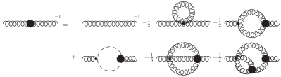
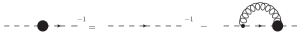
Figure 1: Dyson-Schwinger equations for the gluon (top) and ghost (bottom) propagators. Internal propagators are dressed, black disks denote dressed vertices, dots denote bare vertices, wiggly lines denote gluons and dashed lines denote ghosts.

The exact set of coupled Dyson-Schwinger equations (DSEs) for the gluon and ghost propagators in Landau gauge Yang-Mills theory is displayed in Fig. 1. In Landau gauge, the ghost and gluon propagators, $D_{G}$ and $D_{\mu\nu}$, are given by

$$D_{G}(p^{2}) =\frac{-G(p^{2})}{p^{2}},$$ (1)

$$D_{\mu\nu}(p^{2}) =\left(\delta_{\mu\nu}-\frac{p_{\mu}p_{\nu}}{p^{2}}\right)\frac{Z(p^{2})}{p^{2}},$$ (2)

where color factors have been suppressed. Their DSEs feature nonperturbative one- and two-loop diagrams on the right-hand side, which all share one property: if the momentum variable $p^{2}$ that enters the diagrams from the outside is complex, poles and branch cuts in the various integrands appear. In principle, this is the reason why a direct solution of these equations on a complex momentum grid is extremely dangerous if not prohibitive, since it automatically implies integration across cuts. In the quark sector of quantum chromodynamics, the situation is somewhat alleviated by the quark mass, which modifies the location of these cuts Windisch:2012sz ; Windisch:2013dxa and allows the calculation in a restricted momentum region. In practical calculations using rainbow-ladder type models, it depends on the type of the model whether cuts are absent Alkofer:2002bp ; Windisch:2016iud , small Maris:1999nt or potentially relevant on a quantitative basis Qin:2011dd . For the gluonic system, such a rainbow-like truncation was employed in Ref. Kaptari:2019ghz . However, due to the structure of the integrals in the gluon propagator DSE, this breaks the self-consistency of the equations, because the propagators one would like to solve for are also contained implicitly in the models. If we want to maintain self-consistency, the appearance and proper treatment of cuts in the integrands seem unavoidable Strauss:2012dg .

We therefore need a different strategy Maris:1995ns , which we call the “ray technique.” We illustrate the basics of the ray technique using a simple massless scalar model with a cubic interaction. The corresponding self-energy diagram in the DSE for the scalar propagator has the same structure as those we consider in Yang-Mills theory but without the complications of Lorentz tensors. The massless propagator is described by

$$D(x)=\frac{Z(x)}{x}$$ (3)

where $x=p^{2}$ and $Z(x)$ is its dressing function. The perturbative one-loop self-energy is given by

$$I(x) =\int_{\Lambda}\frac{d^{d}q}{(2\pi)^{d}}\frac{1}{q^{2}(p+q)^{2}}\,,$$

$$\rightarrow\int_{0}^{\Lambda^{2}}dy\,y^{\frac{d-2}{2}}\int_{0}^{\pi}d\theta(\sin{\theta})^{d-2}\frac{1}{y\,z}\,,$$ (4)

where $y=q^{2}$, $z=(p+q)^{2}=x+y+2\sqrt{x\,y}\,\cos{\theta}$ and constant factors were dropped in the second line for brevity. This notation is kept throughout this paper, i.e., the external momentum squared is $x$, the internal one squared is $y$ and the squared combined momentum is $z$. We regularize the integral by the $O(d)$ symmetric UV cutoff $\Lambda$ for the radial part. For now, we also keep the dimension $d$ general.

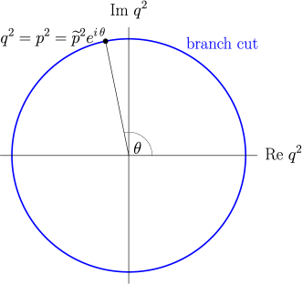
Figure 2: The branch cut (blue) in the $y$ plane created by the angle integration. The end points are at $y=q^{2}=p^{2}$.

Clearly, the integrand is singular for $z=0$. For fixed external momentum $x$, this singularity is located at $y=x\,\exp(\pm 2\,i\,\theta)$. The angular integration over $\theta$ then leads to a branch cut in the $y$ plane with the end points at $y=x$. As is visualized in Fig. 2, the branch cut lies on a circle with $|y|=|x|$. There is only one point at $\arg{x}=\arg{y}$ where the cut is open. For any nonreal or negative $x$, the usual integration path of $y$ along the positive real axis is now forbidden, since it would cross the cut. To avoid this problem, one needs to deform the integration path from $y=0$ to $y=\Lambda^{2}$ such that it goes through the opening at $y=x$ in between. However, it depends on the dimension (and in the most general case on the details of the integral kernels and the dressing functions) whether the opening is suitably finite and the path is safe. The crucial factor here is the behavior of the integrand at the boundaries of the angular integration. In our example, the perturbative treatment of the scalar theory, singularities for $|y|=|x|$ appear in $d=2$ dimensions which is just a manifestation of perturbation theory being ill-defined for the massless theory in two dimensions. In higher dimensions, the path deformation is possible.

For Yang-Mills theory, the situation is more complicated. Let us first have a closer look at the DSE for the ghost propagator which contains the ghost-gluon vertex as the only quantity beyond the propagators. It is a very well-known object with only one dressing function $D^{A\bar{c}c,T}$ contributing to the integrand due to the transversality of the gluon propagator in Landau gauge. The behavior of the integrand of the angular integral is then controlled by a momentum-dependent kinematic kernel times the dressing functions of the vertex and, depending on the momentum routing, the dressing of the ghost or the gluon propagator. For the latter situation we obtain

$$I(x) \rightarrow\int_{0}^{\Lambda^{2}}dy\,y^{\frac{d-2}{2}}\frac{G(y)}{y}$$ (5)

$$\int_{0}^{\pi}d\theta(\sin{\theta})^{d-2}\,\frac{(\sin{\theta})^{2}\,Z(z)\,D^{A\bar{c}c,T}(x,y,z)}{z}\,,$$

where the extra factor $(\sin{\theta})^{2}$ in the kernel stems from the contraction of the gluon with the two vertices. This angular integral is finite at $|y|=|x|$ in any dimension provided the vertex dressing function $D^{A\bar{c}c,T}$ does not develop a strong singularity for $z=0$ that overcompensates for the kernel and the well-known infrared behavior $Z(z)\rightarrow 0$ of the gluon dressing function. The information we have about the ghost-gluon vertex does not support the existence of such a problematic singularity (e.g., Refs. Sternbeck:2007ug ; Cucchieri:2007zm ; Alkofer:2008jy ; Alkofer:2008dt ; Fischer:2009tn ; Huber:2012kd ; Aguilar:2013xqa ; Pelaez:2013cpa ; Williams:2015cvx ; Cyrol:2016tym ; Mintz:2017qri ; Aguilar:2018csq ; Huber:2018ned ; Huber:2020keu ). A similar situation arises for the ghost loop in the gluon propagator DSE. For the gluon loop, however, terms proportional to $1/z^{2}$ appear (see, e.g., Ref. Fischer:2002hn for explicit expressions). Fortunately, these are countered by the presence of at least one factor of $Z(z)\rightarrow 0$ in the integrand. Thus, again, provided the three-gluon vertex does not develop a strong singularity at $z=0$, the integral is finite and the path deformation works. It should be stressed here that the crucial momentum variable $z$ affects only one leg of the three-gluon vertex. The relevant divergence structure is thus that of one momentum going to zero and not the global IR behavior of the three-gluon vertex. Luckily, the former divergences were found to be only weak Alkofer:2008jy ; Alkofer:2008dt ; Fischer:2009tn .

One can show as well that the path deformation works for the two-loop diagrams. Since below we will deal with a truncation involving one-loop diagrams only, we refrain from going into detail here and refer to Ref. Huber:2018ned for details on their structure. We furthermore wish to emphasize that the problem of potential singularities at $|y|=|x|$ is absent for massive propagators such as quarks. Due to the finite mass one then encounters an opening of the branch cut of finite size Windisch:2012sz ; Windisch:2013dxa .

Additional problems may be encountered if dressing functions present under the integral develop poles or branch cuts at momenta other than $z=0$ probed by the integration. In principle, this leads to additional constraints on the integration contour. A typical case is a pole in a propagator $D(x)$ at complex momentum $x_{0}$. If this propagator only appears under the radial integral, then either the path may be deformed around the pole, or a corresponding residue needs to be taken into account. The situation is worse if the propagator also depends on the angle, i.e. if we have $D(z)$ or more general momentum arguments. The singularity condition is then $z=x_{0}$ and corresponds to the case of a massive propagator with mass $m=-x_{0}$. Thus in principle it can be dealt with analogously, as already discussed above and in Refs. Windisch:2012sz ; Windisch:2013dxa . In practice, however, this solution is very hard to implement in a self-consistent way in numerically demanding situations such as the coupled system of ghost and gluon propagators.

Setting these potential additional problems aside for the moment, it remains to be discussed how the integration contour is chosen in practice. A typical integration path is shown in Fig. 3. The integration contour runs along a radial “ray” and is then continued to the cutoff $\Lambda^{2}$ by a second curve which we call “arc“. The precise form of the arc is not so relevant in practice. All details concerning the numerical implementation of the ray technique are discussed in Appendix A.

Figure 3: Integration contour (red) from $0$ to the cutoff $\Lambda^{2}$ via the opening in the branch cut (blue, dashed) at $q^{2}=p^{2}$.

III Truncation and renormalization of the gluon and ghost propagator DSEs

In this work, we are primarily interested in a conceptual study of the gluon propagator at complex momenta. Thus, although the two-loop diagrams in Fig. 1 are quantitatively important on a 20 % level Huber:2016tvc ; Huber:2020keu , we neglect them to avoid substantial technical complications. The tadpole diagram is dropped as well because it vanishes in the renormalization we employ. This truncation leaves us with the system depicted in Fig. 4. This system is closed once the dressed ghost-gluon and three-gluon vertices are known. It is well known Schleifenbaum:2004id ; Sternbeck:2007ug ; Cucchieri:2007zm ; Alkofer:2008jy ; Alkofer:2008dt ; Fischer:2009tn ; Huber:2012kd ; Aguilar:2013xqa ; Pelaez:2013cpa ; Williams:2015cvx ; Cyrol:2016tym ; Mintz:2017qri ; Aguilar:2018csq ; Huber:2018ned ; Huber:2020keu that the ghost-gluon vertex only receives small nonperturbative corrections. Therefore, we take it as bare in our conceptual study. For the three-gluon vertex we tested several models that will be described in the next subsection. The second part of this section describes the renormalization procedure.

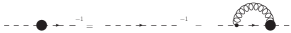
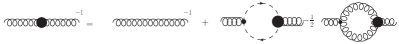
Figure 4: The ghost (top) and the truncated gluon (bottom) propagator DSEs.

III.1 The three-gluon vertex

The three-gluon vertex was studied in various approaches, ranging from lattice simulations Sternbeck:2005tk ; Sternbeck:2006rd ; Cucchieri:2008qm ; Athenodorou:2016oyh ; Duarte:2016ieu ; Sternbeck:2017ntv ; Boucaud:2017obn ; Maas:2020zjp to effective models using a massive gluon propagator Pelaez:2013cpa to functional equations Alkofer:2008jy ; Alkofer:2008dt ; Aguilar:2013vaa ; Blum:2014gna ; Eichmann:2014xya ; Cyrol:2016tym ; Aguilar:2019jsj ; Huber:2020keu ; Aguilar:2020yni . From these studies, the nonperturbative properties for spacelike momenta are quite well understood. In particular, a suppression at intermediate momenta is seen, and the dressing of the tree-level tensor structure even becomes negative. However, the zero crossing is at rather low momenta which are difficult to reach in lattice calculations.

Here we use a model for the three-gluon vertex which also includes a term that restores the correct renormalization group behavior of the gluon propagator. Note that this is only necessary because we discarded the two-loop terms in the gluon propagator DSE. For more elaborate truncations, the correct renormalization group behavior is obtained automatically; see Refs. Huber:2020keu ; Huber:2017txg ; Huber:2018ned . The vertex model is restricted to the tree-level tensor and parametrized as

$$\Gamma {}^{AAA,abc}_{\mu\nu\rho}(p,q,r)=$$

$$\quad i\,g\,f^{abc}\Gamma^{AAA,(0)}_{\mu\nu\rho}(p,q,r)\widetilde{C}^{AAA}(p^{2},q^{2},r^{2}),$$ (6)

where $\Gamma^{AAA,(0)}_{\mu\nu\rho}(p,q,r)$ is the Lorentz tensor of the tree-level vertex.

We tested various forms for $\widetilde{C}^{AAA}(p^{2},q^{2},r^{2})$ which are detailed in Appendix C. As the results for the gluon and ghost propagators are qualitatively very similar for these models, we choose one representative for illustration in plots. This model reads

$$\widetilde{C}_{1}^{AAA}(x,y,z)=\frac{1}{Z_{1}}\frac{G(\overline{p}^{2})^{2-2a/\delta-4a}}{Z(\overline{p}^{2})^{2+2a}}.$$ (7)

$Z_{1}$ is the renormalization constant of the three-gluon vertex, $\delta=-9/44$ is the anomalous dimension of the ghost propagator and $a$ is a parameter that determines the IR behavior of the model. Note that in the UV $a$ drops out due to the scaling relation $1+2\delta+\gamma=0$ of the anomalous dimensions $\delta$ and $\gamma$ of the ghost and gluon propagators, respectively. The vertex model is a reparametrization of the model introduced in Ref. Huber:2012kd without the IR part and corresponds to a Bose-symmetrized version of the model from Ref. Fischer:2002hn . The non-Bose-symmetric version is recovered by replacing the dressings as $G(\overline{p}^{2})^{2}\rightarrow G(y)G(z)$ and $Z(\overline{p}^{2})^{2}\rightarrow Z(y)Z(z)$. This version was used in Ref. Strauss:2012dg and also tested here. Again, though, we did not find any qualitative differences.

The IR behavior of this model is determined by the parameter $a$. Originally, $a=3\delta$ was used which makes the expression IR finite for the scaling solution. Here, we solve for a decoupling solution for which $\widetilde{C}_{1}^{AAA}(x,y,z)$ is IR divergent with $a=3\delta$. One way to circumvent this is to use $a=-1$ instead. This removes the gluon dressing function from the model. An alternative way is to modify the momentum argument by adding a small scale $\Lambda_{\text{IR}}^{2}$. We do so by setting $\overline{p}^{2}=(x+y+z+\Lambda_{\text{IR}}^{2})/2$ with $\Lambda_{\text{IR}}^{2}\in[0,0.01]\,\text{GeV}^{2}$. In the plots shown in Sec. IV, we used $a=3\delta$ with $\Lambda_{\text{IR}}^{2}=0$. However, we checked that the results from the two methods are qualitatively the same.

In this model, the analytic behavior of the three-gluon vertex is completely determined by the analytic structure of the propagator dressing functions. As we found that for the given truncation the gluon propagator seems to have a singular point in the complex plane, we wanted to remove its influence on the vertex. The corresponding models are discussed in Appendix C. While these adaptations do have quantitative effects, all qualitative aspects remain the same. Thus, we conclude that our qualitative results are robust against changes within a large class of three-gluon vertex models, but we stress that our analysis only holds for this class.

III.2 Renormalization

The propagator DSEs are renormalized via a momentum-subtraction scheme. For the ghost propagator DSE this leads to

$$G(p^{2})^{-1}=G(s)^{-1}+\Sigma_{G}(p^{2})-\Sigma_{G}(s).$$ (8)

$G(s)$ denotes the ghost dressing function at an (infrared) subtraction scale $s$ and $\Sigma_{G}(p^{2})$ is the ghost self-energy. The value chosen for $G(s)$ selects a particular solution from a one-parameter family of possible ones; for details see Ref. Fischer:2008uz . To be able to perform the subtraction ray by ray we need to analytically continue the value of $G(s)$ from ray to ray. We do so using the Cauchy-Riemann condition, see Eq. (10) below and Appendix A for details.

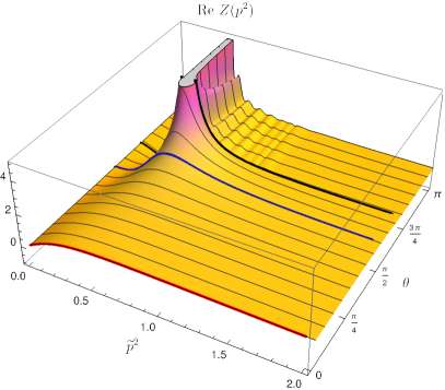
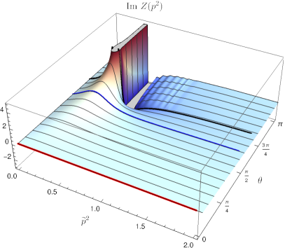
Figure 5: Real (left) and imaginary (right) gluon dressing function shown in the complex momentum plane with $p^{2}=\tilde{p}^{2}e^{i\theta}$. The blue line is at $\theta=\pi/2$ and the red line is the Euclidean result. The black line corresponds to a ray close to the singular point.

For the gluon propagator DSE, the subtraction point needs to be chosen at large momenta for numerical stability. The hard UV cutoff employed in our calculations breaks gauge covariance and leads to additional quadratic divergences in the gluon propagator DSE. Several methods to remove them exist; see Ref. Huber:2014tva and references therein for details. Such a procedure can entail ambiguities and should thus be considered as part of the model input. However, a unique subtraction might be possible with more elaborate truncations Huber:2020keu . Since the present truncation scheme is constructed for qualitative tests, we use a simple but effective subtraction scheme that modifies the integrand of the gluon loop appropriately Fischer:2002hn ; Fischer:2002eq . We also tested other methods. For one, instead of subtracting the overall divergence in the gluon loop, we split the subtraction between ghost and gluon loops Huber:2012kd . For another one, we used a second renormalization condition Meyers:2014iwa ; Huber:2017txg which already proved very useful elsewhere Huber:2020keu . It turns out that the second renormalization condition can be chosen such that both procedures lead to almost similar results.

Finally, it remains to set the physical scale of our results. We do so by matching the gluon dressing function to corresponding lattice results Sternbeck:2006rd in the region above 1 GeV. Thus, we inherit the scale setting used on the lattice.

IV Results

IV.1 Baseline setup

In this section we first present results for what we call “baseline setup.” It is defined by fixed values for the renormalization conditions, the subtraction method of quadratic divergences in the gluon loop and the three-gluon vertex model from Eq. (7) with $a=3\delta$. More details including computational parameters are explained in Appendix A. Variations and tests of this setup are presented in the subsequent subsections.

The gluon dressing function is shown in Fig. 5 as a function of the radial and angular parts of the complex variable $x=p^{2}=\tilde{p}^{2}e^{i\theta}$. In the first quadrant, the calculation works without problems. However, in the second quadrant, the bump in the gluon dressing function at $\tilde{p}^{2}\approx 0.5$ starts to rise appreciably, however, without becoming singular. Beyond a certain value of $\theta$, it flattens again and remains finite until the negative squared momentum axis. This behavior was seen before in a slightly different setup and with less precise numerics Strauss:2012dg and was interpreted as the gluon being regular at complex momenta. However, with the improved numerical treatment followed in this work, we clearly observe oscillations in the solution, which may hint towards numerical artifacts. These signals and the strong rise could also indicate that we may have hit a singular point beyond which the ray technique is no longer applicable. We tried to take this finding into account by modifying the integration path appropriately (cf. the discussion in Sec. II), but then we loose the advantage of the ray technique that we do not need to know the dressing function in unknown regions, and we did not succeed in improving the results in this way. Thus, from this plot we concluded that our results probably cannot be trusted beyond that point and that we may have hit a singularity. We corroborated this conclusion further using various tests that will be detailed below in Sec. IV.2.

Our results for the ghost dressing function in the baseline setup are shown in Fig. 6. In contrast to the gluon propagator, we do not see any drastic changes in the dressing functions. The real part of the ghost is smooth throughout the complex momentum plane, whereas the imaginary part develops a negative bump at the same scale at which the gluon rises drastically. However, since the ghost and the gluon equations are directly coupled, the results for the ghost dressing should only be considered trustworthy up to the location of the potentially singular point in the gluon dressing function.

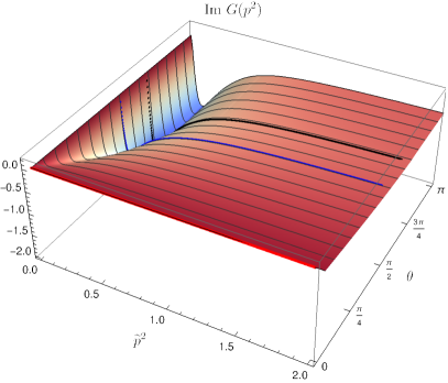
Figure 6: Real (left) and imaginary (right) ghost dressing function. The blue line is at $\theta=\pi/2$ and the red line is the Euclidean result. The black line corresponds to a ray close to the singular point.

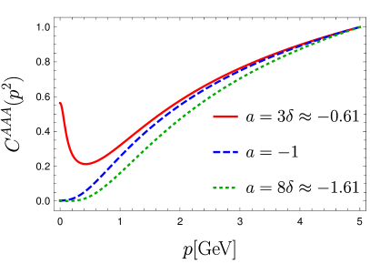
Figure 7: Three-gluon vertex dressing function for the vertex model (7) with different values for the parameter $a$ and $\Lambda_{\text{IR}}^{2}=0.01$.

The reason for the appearance of the potential singularity is not clear. In particular, it cannot be understood in simple terms similar to the Cutkosky rules Cutkosky:1960sp ; Dudal:2010wn which allow to determine the position of a branch cut from the masses of the propagators in a Feynman diagram. In the language of contour deformation, a branch cut in the external momentum arises when the integration path cannot be deformed continuously for two values of $p^{2}$, see Ref. Windisch:2013dxa for details. This is, however, not the case here.

IV.2 Variations

Since the origin of the potential singularity thus seems to be dynamic, we tried to vary our setup to investigate the influence on the existence and position of the singular point. We attempted the following variations of the baseline setup:

• We tried several modifications of the three-gluon vertex model. The corresponding expressions are listed in Appendix C. In addition, we varied the parameter $a$ in the model between $8\delta\approx-1.61$ and $3\delta\approx-0.61$. The effect of this is discussed below.

• We tested alternative methods to subtract quadratic divergences as discussed in Sec. III.2.

• We varied the renormalization condition $G(0)$ of the ghost propagator to obtain different decoupling solutions.

Most variations did not lead to a qualitative change of our results and we do not discuss them further. Different values for $G(0)$ only led to small quantitative changes in the position of the singularity. A larger effect was observed from the employed three-gluon vertex model. In particular, the position of the potentially singular point in the complex momentum plane for the gluon propagator depends on the details of the vertex model. Varying the parameter $a$, cf. Fig. 7, we observed that the point moves closer to the real axis (and at the same time closer to the origin) when the parameter $a$ was lowered. Lowering $a$ as far as $a=8\delta\approx-1.61$, we were able to move the potential singularity almost onto the real axis. This, however, happens at the expense that the gluon dressing function at real spacelike momenta becomes unrealistically flat. We therefore did not lower $a$ further.

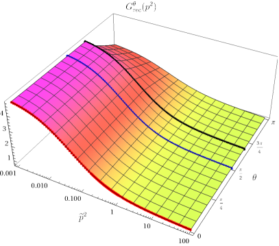
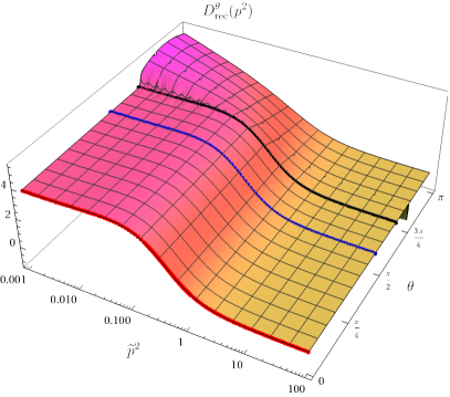
Figure 8: Reconstruction of the ghost dressing function (left) and the gluon propagator (right) from the solution on the rays. The blue line is at $\theta=\pi/2$ and the red line is the Euclidean result. The thick black line marks the ray where the reconstruction begins to fail.

IV.3 Tests

A propagator can be calculated in the complete complex plane from the spectral density $\rho(s)$ via

$$D(p^{2})=\int_{0}^{\infty}ds\frac{\rho(s)}{p^{2}+s}$$ (9)

if no poles at complex momenta exist; see also Appendix B. The inverse task of extracting the spectral density from the propagator given at Euclidean momenta is an ill-posed inverse problem Hansen:2010dip . This is reflected in the necessity of some form of bias in these methods and a large sensitivity of the results to the precision of the input. The direct calculation performed here, on the other hand, does not have these intrinsic problems. Rather, the main challenges are of a numeric nature; see Appendix A. In particular, the global nature of analyticity can be problematic, viz., the analytic properties of a function are encoded in the behavior of the function on any region of the complex plane. Hence, the propagation of errors has to be under control and it is important to check that the numeric calculation does not interfere with analyticity. In this section, we describe several possibilities for such checks and apply them to our results.

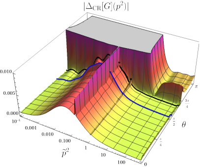
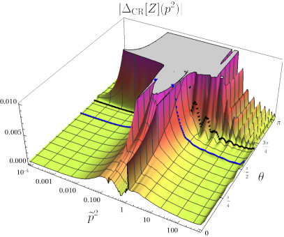
Figure 9: Test of the Cauchy-Riemann condition Eq. (11) for the ghost (left) and gluon (right) dressing functions. The two ridges for fixed $\widetilde{p}^{2}$ are artifacts not related to a failure of analyticity (see main text).

One direct possibility for such a check is provided by Cauchy’s integral formula. We use it to reconstruct the propagators for real and spacelike momenta from any ray and monitor the quality of the reconstruction. The details for this procedure are listed in Appendix B.

We performed this reconstruction on all rays used for the calculation of the gluon propagator and ghost dressing function. For the baseline setup, the reconstructed functions are shown in Fig. 8. For guidance, we also plot the Euclidean result (in red at $\theta=0$). The reconstruction works very well in the first quadrant ($\theta\leq\pi/2$) and some way into the second quadrant until it fails on the ray marked with a thick black line. Beyond this ray, it fails completely. Again, this indicates the appearance of a singularity in the complex plane at or around the ray in black.

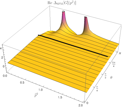
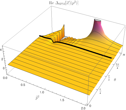
Figure 10: Comparison of the direct calculation with the Schlessinger extrapolation using Eq. (12) for the real parts of the ghost (left) and gluon (right) dressing functions. For the imaginary parts, the qualitative aspects are similar.

Another possibility for a check uses the Cauchy-Riemann equations which relate the real and imaginary parts of analytic functions. In polar coordinates they can be written as

$$\frac{\partial f(x)}{\partial r}=\frac{1}{i\,r}\frac{\partial f(x)}{\partial\theta}$$ (10)

where $x=r\,e^{i\,\theta}$. We can use this to test the analyticity of our results by monitoring

$$\Delta_{\text{CR}}[f](x)=\frac{\partial f(x)}{\partial r}-\frac{1}{i\,r}\frac{\partial f(x)}{\partial\theta}.$$ (11)

We approximate the derivatives by finite differences which leads to its numeric deviations on its own. The results are shown in Fig. 9. Again, we find small deviations for the ghost and gluon propagators (cf. the scale of the $z$ axis) up to the singular point in the second quadrant beyond which the Cauchy-Riemann equations are clearly no longer fulfilled. The two ridges are artifacts from splitting the grid for the dressing functions as discussed in Appendix A.

Having collected ample evidence that our results are analytic until we hit a potential singularity in the second quadrant, we turn the situation around and test the reliability of extrapolating the results from the spacelike axis using the analytic continuation from a Padé approximant. Specifically, we use the Schlessinger point method Schlessinger:1968spm which provides a pointwise exact description of the data. As input, we use a random subset of momentum points on the positive and real momentum axis. Note that this test has been performed already in Ref. Binosi:2019ecz for one of the truncations that we also used here. There, indeed a singularity in the second quadrant was found. Here, we check whether this finding persists for all truncations considered in this work and, even more important, whether the results from the Schlessinger point method agree quantitatively with the explicit results from solving the DSEs in the complex momentum plane.

We compare the direct calculation and the Schlessinger point method by plotting the ratio

$$\Delta_{\text{SPM}}[f](x)=\frac{f(x)}{f_{\text{SPM}}(x)},$$ (12)

where $f_{\text{SPM}}(x)$ is the function as obtained from the Schlessinger point method. This is shown in Fig. 10. The plots confirm that up to the potentially singular point the two methods agree quite well. Next, we compare the positions of the singular points found by the two methods for the gluon propagator. To this end, we follow a simple procedure. For a given subset of input momentum points on the real and positive momentum axis, we calculate the pole positions analytically from the coefficients of the Schlessinger point method. Poles with small residues are discarded as artifacts. For a final estimate of pole positions, we sample several subsets of the Euclidean data. This method is not as elaborate as the one introduced in Ref. Binosi:2019ecz , where the sample of input points is optimized based on the quality of the reconstruction from the spectral function, but quite effective for the present purpose. For the baseline setup, we find that the position of the pole indeed agrees very well with our expectation from the rise of the dressing function, with the location of the breakdown of reconstruction and with the region of the breakdown of the Cauchy-Riemann test. We indicate the location of the pole extracted from the Schlessinger method by a thick black line in Figs. 5, 6, 8, 9 and 10.

Thus, the combined evidence of all methods clearly points towards a singularity in the gluon dressing function at complex momenta. We observed the same quantitative agreement between the pole location predicted by the Schlessinger method and the explicit results from the ray method for all truncations studied in this work.

V Summary

In this work, we studied the analytic structure of the gluon and ghost propagators of Landau gauge Yang-Mills theory from a coupled set of Dyson-Schwinger equations. Using the ray technique, we were able to solve the equations for a region of complex squared momenta that extended well into the second quadrant. We continuously checked our calculation by a variety of other methods, namely by (i) reconstruction algorithms using our solutions to reconstruct the propagators on the spacelike real momentum axis, (ii) the Cauchy-Riemann equations, and (iii) the Schlessinger point method which provides rational functions for the analytic continuation that can be compared with our explicit results. All of these methods agree very well up to a certain ray in the second quadrant. At this point, we encountered a steep rise in the gluon dressing function at the same location where the Schlessinger method predicts a pole. Thus, the combined evidence of both methods strongly suggests the presence of a nonanalytic structure in the complex plane. Due to the less precise numerics available at the time, this structure was not recognized as a singularity in Ref. Strauss:2012dg .

We studied the properties of this singularity and noted that within our truncation, the details of the model for the three-gluon vertex are most relevant for its location, whereas other technical details such as the renormalization procedure matter much less. Since in this study the three-gluon vertex is modeled in terms of the propagators, we cannot make a final statement about the existence or nonexistence of such a pole.

It will be important in the future to further check the dependence of the analytic structure on the gluon interaction. In this respect, it is highly relevant to improve this calculation with better input for the three- and four-gluon vertices, e.g. by using explicit input from solutions of their respective DSEs.

Appendix A Techniques used to solve the DSEs numerically

To extract a high-quality numerical solution of the coupled system of DSEs for the gluon dressing function $Z(p^{2})$ and the ghost dressing function $G(p^{2})$ in the complex $p^{2}$ momentum plane, we employ a variety of numerical tools that are described in some detail in the following. Some of these have been already used in a previous publication Strauss:2012dg .

A.1 The grid

As explained in Sec. II, we solve the DSEs on a grid of “rays” and “arcs”. Each ray extends radially outwards from the origin to a fixed momentum cutoff at $p^{2}=e^{i\theta}\Lambda_{1}^{2}$, where $\theta$ denotes the angle between the ray and the positive real axis. From this point on, the “arc” connects the ray with the real axis along a path given by

$$p^{2}(t) =e^{i\theta(1-t)}\left(\Lambda_{1}^{2}+(\Lambda^{2}-\Lambda_{1}^{2})t\right)$$ (13)

with $t\in[0,1]$. Thus, we have to deal with two different cutoff scales, $\Lambda_{1}$ and $\Lambda$, which are chosen to be close to each other; see Tab. 1. For the grid of rays we typically use 181 rays that cover the complex plane from $\theta=0$ to $\pi-\epsilon$. We also tested using 361 rays or 91 rays instead but did not find any significant influence on the final results. On the real axis, the corresponding ray and arc are of course collinear and merge into a straight line integration path.

A.2 Representation of the dressing functions

The integration paths in the DSEs are along the rays and along the arcs. Under the integrals of the DSEs, we encounter two different types of arguments in the dressing functions $Z$ and $G$: on the one hand, there is the integration momentum denoted by $q^{2}=y$. On the other hand, there is the squared difference between external momentum $p$ and integration momentum $q$ denoted by $(q-p)^{2}=z$. The external momenta $p^{2}=x$ are distributed over the rays, while the integration momenta can be on the rays and the arcs. If $y$ is on a ray, the squared differences, $z$, are also on the rays or their extensions. When $y$ is on an arc, however, $z$ can also take values elsewhere in the complex plane, see Fig. 11 for two examples.

To carry out the integrations on the right-hand side of the DSE, we need the dressing functions $Z$ and $G$ on all these points. In the following we explain in detail how we manage this. Let us first deal with the rays. On each ray, we represent the real part and the imaginary part of $Z$ and $G$ separately by an expansion in terms of Chebyshev polynomials. Such a representation was introduced in Ref. Atkinson:1997tu and has been used in many calculations since. Chebyshev expansions work very well with smooth functions. It is therefore advantageous to perform these expansions on a logarithmic grid for the logarithm of the function to be expanded. For a function $f(x)$ this amounts to

$$f(x)=\exp{\left(\sum_{i=0}^{N-1}t_{i}(x)R_{i}\right)}+i\exp{\left(\sum_{i=0}^{N-1}t_{i}(x)I_{i}\right)}\,.$$ (14)

The $t_{i}$ are the Chebyshev polynomials and the $R_{i}/I_{i}$ are the respective coefficients.

As it turns out, our solutions are indeed smooth enough in the infrared and the ultraviolet momentum regions. However, in a short interval at intermediate momenta, we encounter large variations on rays in the second quadrant of the complex $p^{2}$ plane. We deal with this situation numerically by splitting the radial distance from the origin on each ray into three intervals, $[\epsilon^{2},x_{1}]$, $[x_{1},x_{2}]$ and $[x_{2},\Lambda_{1}^{2}]$. Here, $\epsilon^{2}$ is an infrared momentum cutoff and $\Lambda_{1}^{2}$ is the ultraviolet momentum cutoff on each ray, already discussed above. The middle interval $[x_{1},x_{2}]$ is bracketed close to the interval where the large variations occur. A set of boundaries that worked for the cases considered in this paper is given in Tab. 1. Furthermore, we optimized the number of Chebyshev polynomials $N_{1}$, $N_{2}$ and $N_{3}$ needed for each interval; the resulting numbers can be found in the table as well. In total, we need to solve for the coefficients of 290 Chebyshev polynomials on each ray, which is a tremendous numerical task.

Parameter	Value(s)
Physical parameters
$G(0)$	5
$Z(s)$	0.38
$s$ [i.u.]	200
$\alpha(\mu^{2})$	1
Computational parameters
	gluon	ghost
$\epsilon^{2}$ [i.u.]	$10^{-5}$	$10^{-5}$
$x_{1}$ [i.u.]	0.2	0.2
$x_{2}$ [i.u.]	1	0.6
$\Lambda_{1}^{2}$ [i.u.]	675	675
$\Lambda^{2}$ [i.u.]	$10^{3}$	$10^{3}$
$N_{1}$	30	15
$N_{2}$	30	15
$N_{3}$	30	25

Table 1: Parameter values used for a typical calculation. Internal units (i.u.) correspond roughly to GeV.

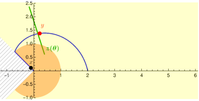
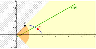
Figure 11: Two examples for the range of values for $z$ (green line) for given values of $x$ and $y$. The blue line represents the integration contour. The orange region is covered by the rays up to the one on which $x$ lies. In the yellow region, the UV extrapolation is applied. When $y$ is on the ray, all possible values for $z$ also lie on the ray (and its UV extrapolation). When $y$ is on the arc as in the plots, the required values for $z$ form a line. The hatched region is only accessible once solutions for rays beyond the one on which $x$ lies have been obtained. The lower half-plane can be accessed by complex conjugation of the dressing functions. The angle approximation corresponds to putting the green points all equal to $y$.

For momenta with absolute values smaller than $\epsilon^{2}$, we use a constant extrapolation for the ghost dressing function $G(p^{2})$ and a constant extrapolation of the gluon propagator function $D(p^{2})=Z(p^{2})/p^{2}$ into the deep infrared. Both extrapolations are well justified from the known behavior of the (decoupling case) dressing functions on the real axis and we assume this to also work in the complex plane. In fact, this can be checked by closely monitoring the behavior of the dressing functions for momenta larger than but close to $\epsilon^{2}$ which was found to agree with the extrapolation.

In the ultraviolet momentum region we used two types of extrapolation: first, one could use the analytic form of the known ultraviolet one-loop running of the dressing functions to extrapolate (see e.g. Ref. Fischer:2002hn ), or, second, one could simply set the functions to a constant value from $\Lambda_{1}$ on. Both procedures lead to similar results and we settled with the simpler second option.

We also need to integrate on the arc. This integration path generates momenta $z$ in all regions of the complex momentum plane. To avoid this, we use the angular approximation $Z(z),G(z)\rightarrow Z(y),G(y)$ on the arc, which is known to work very well for ultraviolet momenta.

For the main calculation, only the dressing functions on the rays are required. However, for some test calculations we also needed the dressing function between the rays. Since our rays are close to each other, we checked that linear interpolation between points on rays sharing a common distance to the origin works very well.

A.3 Numerical integration and iteration

For the numerical integration, some points require special attention which we discuss below. For the radial integration we use an ordinary Gauss-Legendre method separating the rays into four regions. For every external momentum $x$ we use the three intervals of the Chebyshev expansion $[\epsilon^{2},x_{1}]$, $[x_{1},x_{2}]$ and $[x_{2},\Lambda_{1}^{2}]$, detailed above. Additionally, we split the one region which contains $x$ into two intervals. Thus, for small $x$, for instance, we have $[\epsilon^{2},x]$,$[x,x_{1}]$ $[x_{1},x_{2}]$, $[x_{2},\Lambda_{1}^{2}]$, with appropriate modifications for intermediate and large $x$. This is important to have many integration points close to the boundaries of the region and close to $x\approx y$, where we pass through the only opening of the branch cut and encounter (depending on the angle) very small $z$ in one of the denominators of the internal propagators. We typically choose 60 integration points in each interval. Another integration region is the interval $[\Lambda_{1}^{2},\Lambda^{2}]$ on the arc. Since we use the angle approximation, this integration is not problematic.

It turns out that the angular integral has to be treated with extra care, since it is related to (the generation of) cuts and branch points as explained in Sec. II. For any given pair of external and loop momenta $x$ and $y$, respectively, the angular integral generates a potentially broad interval of values of $z$. To treat the evaluation of $Z(z)$ and $G(z)$ in a similar manner as with argument $y$, we perform the following procedure: for any pair of $x$ and $y$, we monitor the interval of $z$ tested by the angular integral. Whenever this interval crosses either $x_{1}$ or $x_{2}$ (the boundaries of the regions discussed above), we split the angular integral at these points. The total of 75 points used for the Gauss-Legendre integration of the angle are then distributed into these regions. We found that splitting the integration intervals for both the radial and angular parts as described above is pivotal, whereas the integration itself is rather stable in the number of points as long as not severely fewer points are used.

Finally, we need to discuss details of the iteration procedure. The solution on the first ray/arc (only real and positive momenta) is obtained with standard techniques. We then use this solution as a starting guess for the second ray/arc combination and iterate until convergence on the second ray is achieved. The solution for the second ray is then used as a starting guess for the iteration on the third ray and so on. As explained in the main text, we renormalize the gluon DSE on the first ray/arc (only real and positive momenta); the corresponding value of $Z_{3}$ remains constant for all other rays. This procedure is not possible for the ghost propagator DSE, since $G(s)$ at the infrared subtraction point $s$ has a special meaning in connection with the family of decoupling solutions. To maintain a connection to one particular member of the class of decoupling solutions dialed by $G(s)$ on the first ray/arc, we use the Cauchy-Riemann condition discussed in Sec. III.2 to determine the (complex) $G(s)$ on each subsequent ray. Since, in particular in the infrared, the rays are very close to each other, the numerical error of this procedure is extremely small (we tested this explicitly on trial functions with various analytic structures in the complex plane).

Appendix B Cauchy’s integral formula and reconstruction

Cauchy’s integral formula can be used to calculate the value of a holomorphic function inside a closed region via knowledge of the function on the boundaries:

$$D(x)=\frac{1}{2\pi i}\oint_{C}dz\frac{D(z)}{z-x}.$$ (15)

From this, one can directly derive the spectral representation of a propagator. Here we repeat this derivation but use different integration paths that correspond to the rays on which we calculate the propagators. This can be used as a test whether the numeric solution still respects analyticity.

In general, the analytic structure of a propagator can contain poles and a cut on the timelike axis. An integration contour of a circle at infinity thus needs to be deformed to take them into account:

$$C=C_{\infty}+C_{c}+C_{p}.$$ (16)

The integral at infinity ($C_{\infty}$) vanishes and only the integrals along the cut ($C_{c}$) and around the poles ($C_{p}$) remain. The latter leads to contributions of the residues of the $n$ poles at $z_{j}$:

$$-\sum_{j}\operatorname*{Res}_{z\rightarrow z_{j}}\frac{D(z)}{z_{j}-x}=\sum_{j}\frac{R_{j}}{x-z_{j}}.$$ (17)

The first minus sign comes from integrating clockwise around the poles. The integral along the cut leads to

$$\frac{1}{2\pi\,i}\left(\int_{-\infty}^{0}dz\frac{D(z+i\,\epsilon)}{z-x}+\int_{0}^{-\infty}dz\frac{D(z-i\,\epsilon)}{z-x}\right)$$ (18)

$$= -\frac{1}{2\pi\,i}\int_{0}^{\infty}ds\frac{D(-s+i\,\epsilon)-D(-s-i\epsilon)}{s+x}$$ (19)

$$= -\frac{1}{\pi}\int_{0}^{\infty}ds\frac{\text{Im}{D(-s)}}{s+x}$$ (20)

$$= \int_{0}^{\infty}ds\frac{\rho(s)}{s+x}.$$ (21)

This is the spectral representation for a propagator already shown in Eq. (9). The spectral density is defined as

$$\rho(s)=-\frac{\text{disc}D(-s)}{2\pi\,i}=-\frac{1}{\pi}\text{Im}D(-s).$$ (22)

One can also change the contour such that it runs from infinity to the origin not along the timelike axis but along a ray at angle $\theta$ (and out at angle $-\theta$), see Fig. 12. We consider the two contributions separately:

$$D^{\theta}_{r}(x) =\frac{1}{2\pi\,i}\left(\int_{\Lambda^{2}\,e^{i\theta}}^{0}dz\frac{D(z)}{z-x}+\int_{0}^{\Lambda^{2}e^{-i\theta}}dz\frac{D(z)}{z-x}\right)$$ (23)

$$=\frac{1}{2\pi\,i}\left(-\int_{0}^{\Lambda^{2}\,e^{i\theta}}dz\frac{D(z)}{z-x}+\int_{0}^{\Lambda^{2}e^{-i\theta}}dz\frac{D(z)}{z-x}\right)$$ (24)

$$=\frac{1}{2\pi\,i}\int_{0}^{\Lambda^{2}}dr\left(\frac{-e^{i\,\theta}D(r\,e^{i\,\theta})}{r\,e^{i\,\theta}-x}+\frac{e^{-i\,\theta}D(r\,e^{-i\,\theta})}{r\,e^{-i\,\theta}-x}\right)$$ (25)

$$=-\frac{1}{\pi}\int_{0}^{\Lambda^{2}}dr\,\text{Im}\left(\frac{e^{i\,\theta}D(r\,e^{i\,\theta})}{r\,e^{i\,\theta}-x}\right).$$ (26)

If $\theta=\pi$, we recover Eq. (9). Since we have a finite cutoff $\Lambda^{2}$, we also add the contribution from the circle segment:

$$D^{\theta}_{a}(x) =\frac{1}{2\pi\,i}\left(\int_{\Lambda^{2}\,e^{-i\theta}}^{\Lambda^{2}\,e^{i\theta}}dz\frac{D(z)}{z-x}\right)$$ (27)

$$=\frac{\Lambda^{2}}{\pi}\int_{0}^{\theta}d\phi\,\text{Re}\left(\frac{e^{i\,\phi}D(\Lambda^{2}\,e^{i\,\phi})}{\Lambda^{2}\,e^{i\,\phi}-x}\right).$$ (28)

The reconstructed propagator is then

$$D^{\theta}_{\text{rec}}(x)=D^{\theta}_{r}(x)+D^{\theta}_{a}(x).$$ (29)

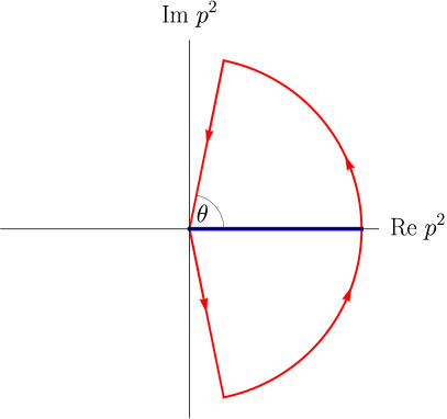
Figure 12: Integration contour (red) to reconstruct the propagator on the positive real axis (blue) from the solution on a ray with angle $\theta$.

Appendix C Three-gluon vertex models

The different vertex models we employed in our studies are detailed here. For convenience, we define an auxiliary function

$$F(x)=\frac{G(x)^{1-a/\delta-2a}}{Z(x)^{1+a}}.$$ (30)

$\delta=-9/44$ is the anomalous dimension of the ghost propagator. The exponents of the dressings are taken such that this function behaves like $(\delta-\gamma)$, which is the anomalous dimension of the three-gluon vertex. The parameter $a$ can be used to modify the IR behavior and was varied for testing.

The baseline vertex is then defined as

$$\widetilde{C}_{1}^{AAA}(x,y,z)=\frac{1}{Z_{1}}F\left(\frac{x+y+z+\Lambda_{\text{IR}}^{2}}{2}\right)^{2}.$$ (31)

This is a Bose-symmetrized version of the one introduced in Ref. Fischer:2002hn with an additional IR scale $\Lambda_{\text{IR}}^{2}$ that serves to avoid the divergence for $a=3\delta$. The exponent accounts for the renormalization group improvement. We use as arguments $x=p^{2}$, $y=q^{2}$ and $z=(p+q)^{2}$ as they actually appear in the gluon loop for external/internal momentum $p/q$. The factor $1/2$ guarantees the correct behavior for large loop momentum.

The integration kernel of the gluon loop contains the gluon dressing functions as $Z(y)Z(z)$. To test the potential influence of and avoid possible problems from these terms, we discarded them in another vertex model and fixed the UV behavior by essentially modifying the exponent of the gluon dressing function from the original model:

$$\widetilde{C}_{6}^{AAA}(x,y,z)=F\left(\frac{x+y+z+\Lambda_{\text{IR}}^{2}}{2}\right)^{2}\frac{Z\left(\frac{x+y+z+\Lambda_{\text{IR}}^{2}}{2}\right)^{2}}{Z(y)Z(z)}$$ (32)

Two variations of this model remove the dependence on the angle by replacing the momentum arguments:

$$\widetilde{C}_{7}^{AAA}(x,y,z)=F\left(\frac{x+y+\Lambda_{\text{IR}}^{2}}{2}\right)^{2}\frac{Z\left(\frac{x+y+\Lambda_{\text{IR}}^{2}}{2}\right)^{2}}{Z(y)Z(z)},$$ (33)

$$\widetilde{C}_{8}^{AAA}(x,y,z)=F\left(\frac{y+\Lambda_{\text{IR}}^{2}}{2}\right)^{2}\frac{Z\left(\frac{y+\Lambda_{\text{IR}}^{2}}{2}\right)^{2}}{Z(y)Z(z)}$$ (34)

The potential poles induced by these arguments are irrelevant for the integration as they are on the negative real axis.

A final model we tested is the one from Ref. Fischer:2002hn which was also used for the previous calculation of the gluon and ghost propagators in the complex plane Strauss:2012dg . It is given by

$$\widetilde{C}_{0}^{AAA}(x,y,z)=\frac{1}{Z_{1}}\frac{(G(y)G(z))^{1-a/\delta-2a}}{(Z(y)Z(z))^{1+a}}.$$ (35)

References

- (1) V. Gribov, “Quantization of Nonabelian Gauge Theories”, Nucl.Phys. B139 (1978) 1.
- (2) D. Zwanziger, “Local and Renormalizable Action From the Gribov Horizon”, Nucl. Phys. B 323 (1989) 513–544.
- (3) M. Stingl, “Propagation Properties and Condensate Formation of the Confined Yang-Mills Field”, Phys. Rev. D 34 (1986) 3863.
- (4) D. Dudal, J. A. Gracey, S. P. Sorella, N. Vandersickel, and H. Verschelde, “A refinement of the Gribov-Zwanziger approach in the Landau gauge: infrared propagators in harmony with the lattice results”, Phys. Rev. D78 (2008) 065047, arXiv:0806.4348 [hep-th].
- (5) R. Alkofer, W. Detmold, C. S. Fischer, and P. Maris, “Analytic properties of the Landau gauge gluon and quark propagators”, Phys. Rev. D70 (2004) 014014, arXiv:hep-ph/0309077.
- (6) P. Lowdon, “Nonperturbative structure of the photon and gluon propagators”, Phys. Rev. D 96 no. 6, (2017) 065013, arXiv:1702.02954 [hep-th].
- (7) P. Lowdon, “Dyson–Schwinger equation constraints on the gluon propagator in BRST quantised QCD”, Phys. Lett. B 786 (2018) 399–402, arXiv:1801.09337 [hep-th].
- (8) A. K. Cyrol, J. M. Pawlowski, A. Rothkopf, and N. Wink, “Reconstructing the gluon”, SciPost Phys. 5 no. 6, (2018) 065, arXiv:1804.00945 [hep-ph].
- (9) Y. Hayashi and K.-I. Kondo, “Complex poles and spectral function of Yang-Mills theory”, Phys. Rev. D 99 no. 7, (2019) 074001, arXiv:1812.03116 [hep-th].
- (10) K.-I. Kondo, M. Watanabe, Y. Hayashi, R. Matsudo, and Y. Suda, “Reflection positivity and complex analysis of the Yang-Mills theory from a viewpoint of gluon confinement”, Eur. Phys. J. C 80 no. 2, (2020) 84, arXiv:1902.08894 [hep-th].
- (11) A. Cucchieri, D. Dudal, T. Mendes, and N. Vandersickel, “Modeling the Gluon Propagator in Landau Gauge: Lattice Estimates of Pole Masses and Dimension-Two Condensates”, Phys. Rev. D 85 (2012) 094513, arXiv:1111.2327 [hep-lat].
- (12) A. Cucchieri, D. Dudal, T. Mendes, and N. Vandersickel, “Modeling the Landau-gauge ghost propagator in 2, 3, and 4 spacetime dimensions”, Phys. Rev. D93 no. 9, (2016) 094513, arXiv:1602.01646 [hep-lat].
- (13) S. W. Li, P. Lowdon, O. Oliveira, and P. J. Silva, “The generalised infrared structure of the gluon propagator”, Phys. Lett. B 803 (2020) 135329, arXiv:1907.10073 [hep-th].
- (14) F. Siringo, “Analytic structure of QCD propagators in Minkowski space”, Phys. Rev. D 94 no. 11, (2016) 114036, arXiv:1605.07357 [hep-ph].
- (15) A. F. Falcão, “Padé Approximants and the analytic structure of the gluon and ghost propagators”. Master thesis, 2020. arXiv:2009.08961 [hep-lat].
- (16) A. F. Falcão, O. Oliveira, and P. J. Silva, “The analytic structure of the lattice Landau gauge gluon and ghost propagators”, arXiv:2008.02614 [hep-lat].
- (17) D. Dudal, O. Oliveira, and P. J. Silva, “Källén-Lehmann spectroscopy for (un)physical degrees of freedom”, Phys. Rev. D89 no. 1, (2014) 014010, arXiv:1310.4069 [hep-lat].
- (18) D. Dudal, O. Oliveira, M. Roelfs, and P. Silva, “Spectral representation of lattice gluon and ghost propagators at zero temperature”, Nucl. Phys. B 952 (2020) 114912, arXiv:1901.05348 [hep-lat].
- (19) D. Binosi and R.-A. Tripolt, “Spectral functions of confined particles”, Phys. Lett. B 801 (2020) 135171, arXiv:1904.08172 [hep-ph].
- (20) M. Haas, L. Fister, and J. M. Pawlowski, “Gluon spectral functions and transport coefficients in Yang–Mills theory”, Phys. Rev. D90 (2014) 091501, arXiv:1308.4960 [hep-ph].
- (21) M. Q. Huber, C. S. Fischer, and H. Sanchis-Alepuz, “Spectrum of scalar and pseudoscalar glueballs from functional methods”, arXiv:2004.00415 [hep-ph].
- (22) M. Q. Huber, “Correlation functions of Landau gauge Yang-Mills theory”, Phys. Rev. D 101 no. 11, (2020) 114009, arXiv:2003.13703 [hep-ph].
- (23) Y. Chen et al., “Glueball spectrum and matrix elements on anisotropic lattices”, Phys. Rev. D73 (2006) 014516, arXiv:hep-lat/0510074 [hep-lat].
- (24) C. J. Morningstar and M. J. Peardon, “The Glueball spectrum from an anisotropic lattice study”, Phys. Rev. D60 (1999) 034509, arXiv:hep-lat/9901004 [hep-lat].
- (25) A. Athenodorou and M. Teper, “The glueball spectrum of SU(3) gauge theory in 3+1 dimension”, arXiv:2007.06422 [hep-lat].
- (26) A. Bashir, L. Chang, I. C. Cloet, B. El-Bennich, Y.-X. Liu, C. Roberts, C. D., and P. Tandy, “Collective perspective on advances in Dyson-Schwinger Equation QCD”, Commun.Theor.Phys. 58 (2012) 79–134, arXiv:1201.3366 [nucl-th].
- (27) G. Eichmann, H. Sanchis-Alepuz, R. Williams, R. Alkofer, and C. S. Fischer, “Baryons as relativistic three-quark bound states”, Prog. Part. Nucl. Phys. 91 (2016) 1–100, arXiv:1606.09602 [hep-ph].
- (28) S. Strauss, C. S. Fischer, and C. Kellermann, “Analytic structure of the Landau gauge gluon propagator”, Phys.Rev.Lett. 109 (2012) 252001, arXiv:1208.6239 [hep-ph].
- (29) P. Maris, “Confinement and complex singularities in QED in three-dimensions”, Phys. Rev. D52 (1995) 6087–6097, arXiv:hep-ph/9508323 [hep-ph].
- (30) A. Windisch, R. Alkofer, G. Haase, and M. Liebmann, “Examining the Analytic Structure of Green’s Functions: Massive Parallel Complex Integration using GPUs”, Comput. Phys. Commun. 184 (2013) 109–116, arXiv:1205.0752 [hep-ph].
- (31) A. Windisch, M. Q. Huber, and R. Alkofer, “On the analytic structure of scalar glueball operators at the Born level”, Phys. Rev. D87 no. 6, (2013) 065005, arXiv:1212.2175 [hep-ph].
- (32) R. Williams, “Vector mesons as dynamical resonances in the Bethe–Salpeter framework”, Phys. Lett. B 798 (2019) 134943, arXiv:1804.11161 [hep-ph].
- (33) A. S. Miramontes and H. Sanchis-Alepuz, “On the effect of resonances in the quark-photon vertex”, Eur. Phys. J. A 55 no. 10, (2019) 170, arXiv:1906.06227 [hep-ph].
- (34) G. Eichmann, P. Duarte, M. Peña, and A. Stadler, “Scattering amplitudes and contour deformations”, Phys. Rev. D 100 no. 9, (2019) 094001, arXiv:1907.05402 [hep-ph].
- (35) L. Kaptari, B. Kämpfer, and P. Zhang, “Modeling the gluon and ghost propagators in Landau gauge by truncated Dyson-Schwinger equations”, Eur. Phys. J. Plus 134 no. 8, (2019) 383.
- (36) A. Windisch, M. Q. Huber, and R. Alkofer, “How to determine the branch points of correlation functions in Euclidean space”, Acta Phys. Polon. Supp. 6 no. 3, (2013) 887–892, arXiv:1304.3642 [hep-ph].
- (37) R. Alkofer, P. Watson, and H. Weigel, “Mesons in a Poincare covariant Bethe-Salpeter approach”, Phys.Rev. D65 (2002) 094026, arXiv:hep-ph/0202053 [hep-ph].
- (38) A. Windisch, “Analytic properties of the quark propagator from an effective infrared interaction model”, Phys. Rev. C95 no. 4, (2017) 045204, arXiv:1612.06002 [hep-ph].
- (39) P. Maris and P. C. Tandy, “Bethe-Salpeter study of vector meson masses and decay constants”, Phys. Rev. C60 (1999) 055214, arXiv:nucl-th/9905056 [nucl-th].
- (40) S.-x. Qin, L. Chang, Y.-x. Liu, C. D. Roberts, and D. J. Wilson, “Interaction model for the gap equation”, Phys. Rev. C84 (2011) 042202, arXiv:1108.0603 [nucl-th].
- (41) M. Q. Huber, A. Maas, and L. von Smekal, “Two- and three-point functions in two-dimensional Landau-gauge Yang-Mills theory: Continuum results”, JHEP 1211 (2012) 035, arXiv:1207.0222 [hep-th].
- (42) A. Sternbeck, L. von Smekal, D. Leinweber, and A. Williams, “Comparing SU(2) to SU(3) gluodynamics on large lattices”, PoS LAT2007 (2007) 340, arXiv:0710.1982 [hep-lat].
- (43) A. Cucchieri, T. Mendes, O. Oliveira, and P. J. Silva, “Just how different are SU(2) and SU(3) Landau propagators in the IR regime?”, Phys. Rev. D76 (2007) 114507, arXiv:0705.3367 [hep-lat].
- (44) R. Alkofer, M. Q. Huber, and K. Schwenzer, “Infrared singularities in Landau gauge Yang-Mills theory”, Phys. Rev. D81 (2010) 105010, arXiv:0801.2762 [hep-th].
- (45) R. Alkofer, M. Q. Huber, and K. Schwenzer, “Infrared Behavior of Three-Point Functions in Landau Gauge Yang-Mills Theory”, Eur. Phys. J. C62 (2009) 761–781, arXiv:0812.4045 [hep-ph].
- (46) C. S. Fischer and J. M. Pawlowski, “Uniqueness of infrared asymptotics in Landau gauge Yang- Mills theory II”, Phys. Rev. D80 (2009) 025023, arXiv:0903.2193 [hep-th].
- (47) M. Q. Huber and L. von Smekal, “On the influence of three-point functions on the propagators of Landau gauge Yang-Mills theory”, JHEP 1304 (2013) 149, arXiv:1211.6092 [hep-th].
- (48) A. Aguilar, D. Ibáñez, and J. Papavassiliou, “Ghost propagator and ghost-gluon vertex from Schwinger-Dyson equations”, Phys.Rev. D87 (2013) 114020, arXiv:1303.3609 [hep-ph].
- (49) M. Pelaez, M. Tissier, and N. Wschebor, “Three-point correlation functions in Yang-Mills theory”, Phys.Rev. D88 (2013) 125003, arXiv:1310.2594 [hep-th].
- (50) R. Williams, C. S. Fischer, and W. Heupel, “Light mesons in QCD and unquenching effects from the 3PI effective action”, Phys. Rev. D93 no. 3, (2016) 034026, arXiv:1512.00455 [hep-ph].
- (51) A. K. Cyrol, L. Fister, M. Mitter, J. M. Pawlowski, and N. Strodthoff, “Landau gauge Yang-Mills correlation functions”, Phys. Rev. D94 no. 5, (2016) 054005, arXiv:1605.01856 [hep-ph].
- (52) B. W. Mintz, L. F. Palhares, S. P. Sorella, and A. D. Pereira, “The ghost-gluon vertex in the presence of the Gribov horizon”, arXiv:1712.09633 [hep-th].
- (53) A. C. Aguilar, M. N. Ferreira, C. T. Figueiredo, and J. Papavassiliou, “Nonperturbative structure of the ghost-gluon kernel”, Phys. Rev. D99 no. 3, (2019) 034026, arXiv:1811.08961 [hep-ph].
- (54) M. Q. Huber, “Nonperturbative properties of Yang-Mills theories”, Phys. Rep. (2020) , arXiv:1808.05227 [hep-ph].
- (55) C. S. Fischer and R. Alkofer, “Infrared exponents and running coupling of SU(N) Yang-Mills theories”, Phys. Lett. B536 (2002) 177–184, arXiv:hep-ph/0202202.
- (56) M. Q. Huber, “Correlation functions of three-dimensional Yang-Mills theory from Dyson-Schwinger equations”, Phys. Rev. D93 no. 8, (2016) 085033, arXiv:1602.02038 [hep-th].
- (57) W. Schleifenbaum, A. Maas, J. Wambach, and R. Alkofer, “Infrared behaviour of the ghost-gluon vertex in Landau gauge Yang-Mills theory”, Phys.Rev. D72 (2005) 014017, arXiv:hep-ph/0411052 [hep-ph].
- (58) A. Sternbeck, E. M. Ilgenfritz, M. Mueller-Preussker, and A. Schiller, “Going infrared in su(3) landau gauge gluodynamics”, Phys. Rev. D72 (2005) 014507, arXiv:hep-lat/0506007.
- (59) A. Sternbeck, “The Infrared behavior of lattice QCD Green’s functions”. PhD thesis, Humboldt-Universität zu Berlin, 2006. arXiv:hep-lat/0609016.
- (60) A. Cucchieri, A. Maas, and T. Mendes, “Three-point vertices in Landau-gauge Yang-Mills theory”, Phys. Rev. D77 (2008) 094510, arXiv:0803.1798 [hep-lat].
- (61) A. Athenodorou, D. Binosi, P. Boucaud, F. De Soto, J. Papavassiliou, J. Rodriguez-Quintero, and S. Zafeiropoulos, “On the zero crossing of the three-gluon vertex”, Phys. Lett. B761 (2016) 444–449, arXiv:1607.01278 [hep-ph].
- (62) A. G. Duarte, O. Oliveira, and P. J. Silva, “Further Evidence For Zero Crossing On The Three Gluon Vertex”, Phys. Rev. D94 no. 7, (2016) 074502, arXiv:1607.03831 [hep-lat].
- (63) A. Sternbeck, P.-H. Balduf, A. Kızılersu, O. Oliveira, P. J. Silva, J.-I. Skullerud, and A. G. Williams, “Triple-gluon and quark-gluon vertex from lattice QCD in Landau gauge”, PoS LATTICE2016 (2017) 349, arXiv:1702.00612 [hep-lat].
- (64) P. Boucaud, F. De Soto, J. Rodríguez-Quintero, and S. Zafeiropoulos, “Refining the detection of the zero crossing for the three-gluon vertex in symmetric and asymmetric momentum subtraction schemes”, Phys. Rev. D95 no. 11, (2017) 114503, arXiv:1701.07390 [hep-lat].
- (65) A. Maas and M. Vujinović, “More on the three-gluon vertex in SU(2) Yang-Mills theory in three and four dimensions”, arXiv:2006.08248 [hep-lat].
- (66) A. Aguilar, D. Binosi, D. Ibáñez, and J. Papavassiliou, “Effects of divergent ghost loops on the Green’s functions of QCD”, Phys.Rev. D89 (2014) 085008, arXiv:1312.1212 [hep-ph].
- (67) A. Blum, M. Q. Huber, M. Mitter, and L. von Smekal, “Gluonic three-point correlations in pure Landau gauge QCD”, Phys. Rev. D 89 (2014) 061703(R), arXiv:1401.0713 [hep-ph].
- (68) G. Eichmann, R. Williams, R. Alkofer, and M. Vujinovic, “The three-gluon vertex in Landau gauge”, Phys.Rev. D89 (2014) 105014, arXiv:1402.1365 [hep-ph].
- (69) A. C. Aguilar, M. N. Ferreira, C. T. Figueiredo, and J. Papavassiliou, “Nonperturbative Ball-Chiu construction of the three-gluon vertex”, Phys. Rev. D99 no. 9, (2019) 094010, arXiv:1903.01184 [hep-ph].
- (70) A. Aguilar, M. Ferreira, and J. Papavassiliou, “Novel sum rules for the three-point sector of QCD”, arXiv:2006.04587 [hep-ph].
- (71) M. Q. Huber, “On non-primitively divergent vertices of Yang–Mills theory”, Eur. Phys. J. C77 no. 11, (2017) 733, arXiv:1709.05848 [hep-ph].
- (72) P. Boucaud et al., “IR finiteness of the ghost dressing function from numerical resolution of the ghost SD equation”, JHEP 06 (2008) 012, arXiv:0801.2721 [hep-ph].
- (73) A. Aguilar, D. Binosi, and J. Papavassiliou, “Gluon and ghost propagators in the Landau gauge: Deriving lattice results from Schwinger-Dyson equations”, Phys.Rev. D78 (2008) 025010, arXiv:0802.1870 [hep-ph].
- (74) C. S. Fischer, A. Maas, and J. M. Pawlowski, “On the infrared behavior of Landau gauge Yang-Mills theory”, Annals Phys. 324 (2009) 2408–2437, arXiv:0810.1987 [hep-ph].
- (75) L. von Smekal, R. Alkofer, and A. Hauck, “The infrared behavior of gluon and ghost propagators in Landau gauge QCD”, Phys. Rev. Lett. 79 (1997) 3591–3594, arXiv:hep-ph/9705242.
- (76) L. von Smekal, A. Hauck, and R. Alkofer, “A solution to coupled Dyson-Schwinger equations for gluons and ghosts in Landau gauge”, Ann. Phys. 267 (1998) 1, arXiv:hep-ph/9707327.
- (77) R. Alkofer, C. S. Fischer, and F. J. Llanes-Estrada, “Vertex functions and infrared fixed point in Landau gauge SU(N) Yang-Mills theory”, Phys.Lett. B611 (2005) 279–288, arXiv:hep-th/0412330 [hep-th].
- (78) M. Q. Huber, R. Alkofer, C. S. Fischer, and K. Schwenzer, “The infrared behavior of Landau gauge Yang-Mills theory in d=2, 3 and 4 dimensions”, Phys. Lett. B659 (2008) 434–440, arXiv:0705.3809 [hep-ph].
- (79) M. Q. Huber and L. von Smekal, “Spurious divergences in Dyson-Schwinger equations”, JHEP 1406 (2014) 015, arXiv:1404.3642 [hep-ph].
- (80) C. S. Fischer, R. Alkofer, and H. Reinhardt, “The elusiveness of infrared critical exponents in Landau gauge Yang-Mills theories”, Phys. Rev. D65 (2002) 094008, arXiv:hep-ph/0202195.
- (81) J. Meyers and E. S. Swanson, “The Gluon Propagator with Two-loop Schwinger-Dyson Equations”, Phys.Rev. D90 (2014) 045037, arXiv:1403.4350 [hep-ph].
- (82) R. Cutkosky, “Singularities and discontinuities of Feynman amplitudes”, J. Math. Phys. 1 (1960) 429–433.
- (83) D. Dudal and M. S. Guimaraes, “On the computation of the spectral density of two-point functions: complex masses, cut rules and beyond”, Phys. Rev. D83 (2011) 045013, arXiv:1012.1440 [hep-th].
- (84) P. C. Hansen, Discrete Inverse Problems: Insight and Algorithms. SIAM, 2010.
- (85) L. Schlessinger, “Use of Analyticity in the Calculation of Nonrelativistic Scattering Amplitudes”, Phys. Rev. 167 no. 3, (1968) 1411.
- (86) D. Atkinson and J. C. R. Bloch, “Running coupling in non-perturbative QCD. I: Bare vertices and y-max approximation”, Phys. Rev. D58 (1998) 094036, arXiv:hep-ph/9712459.