Improved Distance Sensitivity Oracles with Subcubic Preprocessing Time

Abstract

We consider the problem of building distance sensitivity oracles (DSOs). Given a directed graph $G=(V,E)$ with edge weights in $\{1,2,\dots,M\}$, we need to preprocess it into a data structure, and answer the following queries: given vertices $u,v\in V$ and a failed vertex or edge $f\in(V\cup E)$, output the length of the shortest path from $u$ to $v$ that does not go through $f$. Our main result is a simple DSO with $\tilde{O}(n^{2.7233}M)$ preprocessing time and $O(1)$ query time. Moreover, if the input graph is undirected, the preprocessing time can be improved to $\tilde{O}(n^{2.6865}M)$. The preprocessing algorithm is randomized with correct probability $\geq 1-1/n^{C}$, for a constant $C$ that can be made arbitrarily large. Previously, there is a DSO with $\tilde{O}(n^{2.8729}M)$ preprocessing time and $\operatorname{polylog}(n)$ query time [Chechik and Cohen, STOC’20].

At the core of our DSO is the following observation from [Bernstein and Karger, STOC’09]: if there is a DSO with preprocessing time $P$ and query time $Q$, then we can construct a DSO with preprocessing time $P+\tilde{O}(n^{2})\cdot Q$ and query time $O(1)$. (Here $\tilde{O}(\cdot)$ hides $\operatorname{polylog}(n)$ factors.)

1 Introduction

Suppose we are given a directed graph $G=(V,E)$, and we want to build a data structure that, given any two vertices $u,v\in V$ and a failure $f$, which is either a failed vertex or a failed edge, outputs the length of the shortest path from $u$ to $v$ that does not go through $f$. Such a data structure is called a distance sensitivity oracle (or DSO for short).

The problem of constructing DSOs is motivated by the fact that real-life networks often suffer from failures. Suppose we have a network with $n$ nodes and $m$ (directed) links, and we want to send a package from a node $u$ to another node $v$. Normally, it suffices to compute the shortest path from $u$ to $v$. However, if some node or link $f$ in this network fails, then our path cannot use $f$, and our task becomes to find the shortest path from $u$ to $v$ that does not go through $f$. Usually, there is only a very small number of failures. In this paper, we consider the simplest case, in which there is only one failed node or link.

The problem of constructing a DSO is well-studied: Demetrescu et al. [6] showed that given a directed graph $G=(V,E)$, there is a DSO which occupies $O(n^{2}\log n)$ space and can answer a query in $O(1)$ time. Duan and Zhang [9] improved the space complexity to $O(n^{2})$, which is optimal for dense graphs (i.e. $m=\Theta(n^{2})$).

Unfortunately, the oracle in [6] requires a large preprocessing time ($O(mn^{2}+n^{3}\log n)$). In real-life applications, the preprocessing time of the DSO is also very important. Bernstein and Karger [2, 3] improved this time bound to $\tilde{O}(mn)$. Note that the All-Pairs Shortest Paths (APSP) problem, which only asks the distances between each pair of vertices $u,v$, is conjectured to require $mn^{1-o(1)}$ time to solve [15]. Since we can solve the APSP problem by using a DSO, the preprocessing time $\tilde{O}(mn)$ is optimal in this sense.

However, if the edge weights are small positive integers (that do not exceed $M$), then the APSP problem can be solved in $\tilde{O}(n^{2.5286}M)$ time [22], which is significantly faster than $O(mn)$ for dense graphs with small weights (e.g. $M=O(1)$). Thus it might be possible to obtain better results than [3] in the regime of small integer edge weights. Weimann and Yuster [21] showed that for any constant $\alpha\in(0,1)$, we can construct a DSO in $\tilde{O}(n^{1-\alpha+\omega}M)$ time. Here $\omega<2.3728639$ is the exponent of matrix multiplication [11]. However, the query time for this oracle is $\tilde{O}(n^{1+\alpha})$, which is superlinear. Later, Grandoni and Williams [13] showed that for every constant $\alpha\in[0,1]$, we can construct a DSO in $\tilde{O}(n^{\omega+1/2}M+n^{\omega+\alpha(4-\omega)}M)$ time, which answers each query in $\tilde{O}(n^{1-\alpha})$ time.

Recently, in an independent work, Chechik and Cohen [4] showed that a DSO with $\operatorname{polylog}(n)$ query time can be constructed in $\tilde{O}(Mn^{2.873})$ time, achieving both subcubic preprocessing time and polylogarithmic query time. The space complexity for their DSO is $\tilde{O}(n^{2.5})$.

1.1 Our Results

In this work, we show improved and simplified constructions of DSOs. We start with an observation.

Observation (Informal).

If we have a DSO with preprocessing time $P$ and query time $Q$, then we can build a DSO with preprocessing time $P+\tilde{O}(n^{2})\cdot Q$ and query time $O(1)$.

For $\alpha=0.2$, the oracle in [13] already achieves $\tilde{O}(n^{2.8729}M)$ preprocessing time and $O(n^{0.8})$ query time. Section 1.1 implies that this query time can be brought down to $O(1)$.

Section 1.1 can be proved by a close inspection of [3]: The algorithm in [3] for constructing a DSO picks $\tilde{O}(n^{2})$ carefully chosen queries $(u,v,f)$, such that the answers of all these queries can be computed in $\tilde{O}(mn)$ time. Then, from these answers, we can easily compute a DSO with query time $O(1)$. If, instead of computing these answers in $\tilde{O}(mn)$ time, we use the given DSO to answer these queries, the preprocessing time becomes $P+\tilde{O}(n^{2})\cdot Q$.

Our main result is a simple construction of DSOs with preprocessing time $\tilde{O}(n^{2.7233}M)$ and query time $O(1)$. If the input graph is undirected, we can achieve a better preprocessing time of $\tilde{O}(n^{2.6865}M)$.

Theorem 1.1.

We can construct a DSO with $\tilde{O}(n^{2.7233}M)$ preprocessing time and $O(1)$ query time. Moreover, if the input graph is undirected, then we can construct a DSO with $\tilde{O}(n^{(3+\omega)/2}M)=\tilde{O}(n^{2.6865}M)$ preprocessing time and $O(1)$ query time. The construction algorithms are randomized and yield valid DSOs w.h.p.

Compared to previous constructions of DSOs, our results have a better dependence on $n$ and are conceptually simpler. Also, the size of our DSO is $\tilde{O}(n^{2})$, which is better than [4]. However, one drawback of our construction is that it cannot handle negative edge weights. (The preprocessing and query time bounds stated above for [21, 13, 4] still hold when the edge weights are integers in $[-M,M]$.)

1.2 Non-unique Shortest Paths

A subtle technical issue is that the shortest paths in $G$ between some vertex pairs may not be unique. Normally, if we perturb every edge weight by a small random value, then we can ensure that shortest paths are unique w.h.p. by the isolation lemma [17, 20]. However, the subcubic-time algorithms for APSP [18, 19, 22] depend crucially on the assumption that edge weights are small integers, so we cannot perform the random perturbation.

Fortunately, there is another elegant way of breaking ties, described in Section 3.4 of [5], that is suitable for our propose. We arbitrarily assign a linear order $\prec$ over the edges of $G$. (For example, we index the edges by distinct numbers in $\{1,2,\dots,m\}$, and define $e_{1}\prec e_{2}$ if the index of $e_{1}$ is smaller than the index of $e_{2}$.) For a path $p$, define the bottleneck edge of $p$ as the smallest edge (w.r.t. $\prec$) in $p$. Let $G^{\prime}$ be a subgraph of $G$ (think of $G^{\prime}=G$ or $G^{\prime}$ is $G$ with some vertex or edge removed), define $w_{G^{\prime}}(u,v)$ as the largest (w.r.t. $\prec$) edge $w\in G^{\prime}$ such that there is a shortest path in $G^{\prime}$ from $u$ to $v$ whose bottleneck edge is $w$. Define $\rho_{G^{\prime}}(u,v)$ to be the following path: If $u=v$, then $\rho_{G^{\prime}}(u,v)$ is the empty path; otherwise, suppose $w_{G^{\prime}}(u,v)$ is an edge from $u^{\star}$ to $v^{\star}$, then $\rho_{G^{\prime}}(u,v)$ is the concatenation of $\rho_{G^{\prime}}(u,u^{\star})$, $w_{G^{\prime}}(u,v)$ and $\rho_{G^{\prime}}(v^{\star},v)$. Note that $\rho_{G^{\prime}}(u,v)$ is always well-defined: we can define $\rho_{G^{\prime}}(u,v)$ inductively, in non-decreasing order of the distance from $u$ to $v$. By a similar induction, we can also prove that $\rho_{G^{\prime}}(u,v)$ is always a shortest path from $u$ to $v$ in $G^{\prime}$.

We list a few properties of this tie-breaking method in the following theorem.

Theorem 1.2.

The following properties of $\rho_{G^{\prime}}(u,v)$ are true:

1. For every $u^{\prime},v^{\prime}\in\rho_{G^{\prime}}(u,v)$ such that $u^{\prime}$ appears before $v^{\prime}$, the portion of $u^{\prime}\rightsquigarrow v^{\prime}$ in $\rho_{G^{\prime}}(u,v)$ coincides with the path $\rho_{G^{\prime}}(u^{\prime},v^{\prime})$.

2. Let $G^{\prime}$ be a subgraph of $G$, suppose $\rho_{G}(u,v)$ is completely contained in $G^{\prime}$, then $\rho_{G^{\prime}}(u,v)=\rho_{G}(u,v)$.

For every vertex $u\in V$, we can compute the collection of paths $\rho_{G^{\prime}}(v,u)$ for every $v\in V$. By (Property a), these paths form a tree rooted at $u$, and we say this tree is the incoming shortest path tree rooted at $u$, denoted as $T^{\sf in}(u)$. Similarly, we can define the outgoing shortest path trees rooted at each vertex, denoted as $T^{\sf out}(u)$. The advantage of this tie-breaking method is:

Theorem 1.3 ([8]).

Given a subgraph $G^{\prime}$, the incoming and outgoing shortest path trees $T^{\sf in}(u)$ and $T^{\sf out}(u)$ for each vertex $u$ can be computed in $\tilde{O}(n^{(3+\omega)/2}M^{1/2})$ time.

For completeness we will prove Theorem 1.2 and 1.3 in Appendix A.

1.3 Notation

We mainly stick to the notation used in [7], namely:

• If $p$ is a path, then $|p|$ denotes the number of edges in it, and $\|p\|$ denotes its length (i.e. the total weight of its edges).

• Let $u,v\in V$, we denote $uv=\rho_{G}(u,v)$, i.e. the unique shortest path from $u$ to $v$ in the original graph. For a vertex or edge failure $f$, we denote $uv\diamond f=\rho_{G-f}(u,v)$, where $G-f$ is the subgraph of $G$ obtained by removing the failure $f$. Note that if $f$ is not in the original path $uv$, then by (Property b), $uv\diamond f=uv$.

• Let $p$ be a path from $u$ to $v$. For two vertices $a,b\in p$ such that $a$ appears earlier than $b$, we say the interval $p[a,b]$ is the subpath from $a$ to $b$, and $p(a,b)$ is the path $p[a,b]$ without its endpoints ($a$ and $b$). If the path $p$ is known in the context, then we may omit $p$ and simply write $[a,b]$ or $(a,b)$. (Property a) implies that, if $p$ is the path $uv$ (or $uv\diamond f$ respectively), then $p[a,b]$ is the path $ab$ (or $ab\diamond f$ respectively).

We define $\mathsf{MM}(n_{1},n_{2},n_{3})$ as the complexity of multiplying an $n_{1}\times n_{2}$ matrix and an $n_{2}\times n_{3}$ matrix. Let $a,b,c$ be real numbers, we define $\omega(a,b,c)$ be the infimum over all real numbers $\alpha$ such that $\mathsf{MM}(n^{a},n^{b},n^{c})=O(n^{\alpha})$. For any real number $r$, we have $\omega(1,1,r)=\omega(1,r,1)=\omega(r,1,1)$ [16], and we denote $\omega(r)=\omega(1,1,r)$.

We also need the following adaptation of Zwick’s APSP algorithm [22] (see also [13, Corollary 3.1]):

Theorem 1.4.

Given an integer $r$ and a directed graph $G=(V,E)$ with edge weights in $\{1,2,\dots,M\}$, we can compute the distances between every pair of nodes whose shortest path uses at most $r$ edges, in $\tilde{O}(rM\cdot\mathsf{MM}(n,n/r,n))$ time.

Proof 1.5 (Proof Sketch).

We simply run the first $\lceil\log_{3/2}r\rceil$ iterations of the algorithm rand-short-path in [22]. The correctness of this algorithm is guaranteed by [22, Lemma 4.2].

2 Constructing a DSO in $\tilde{O}(n^{2.7233}M)$ Time

In this section, we prove Theorem 1.1.

See 1.1

Given an integer $r$ and a graph $G=(V,E)$, we define an $r$-truncated DSO to be a data structure that, when given a query $(u,v,f)$, outputs the value $\min\{\|uv\diamond f\|,r\}$. In other words, an $r$-truncated DSO is a DSO which only needs to be correct when the path $uv\diamond f$ has length at most $r$. If this length is greater than $r$, it outputs $r$ instead.

Inspired by Zwick’s APSP algorithm [22], our main idea is to compute an $r$-truncated DSO for every $r=(3/2)^{i}$. Our high-level strategies for small $r$ and large $r$ are completely different as described below.

When $r$ is small, the sampling approach in [21, 13] already suffices. Fix a particular query $(u,v,f)$, we assume that $f$ is a vertex failure, and $\|uv\diamond f\|\leq r$. In particular, since the edge weights are positive, there are at most $r+1$ vertices in the path $uv\diamond f$. Suppose we sample a graph by discarding each vertex w.p. $1/r$. With probability $\Omega(1/r)$, the resulting graph would “capture” this query in the sense that $f$ is not in it but $uv\diamond f$ is completely included in it. Therefore, if we take $\tilde{O}(r)$ independent samples, and compute APSP for each sampled subgraph, we can deal with every vertex-failure query w.h.p. If $f$ is an edge failure, we simply discard every edge (instead of vertex) in every subgraph w.p. $1/r$, and we can still deal with every edge-failure query w.h.p.

For large $r$, our idea is to compute a $(3/2)r$-truncated DSO from an $r$-truncated DSO. More precisely, given an $r$-truncated DSO with $O(1)$ query time, we can compute a $(3/2)r$-truncated DSO with $\tilde{O}(Mn/r)$ query time as follows. First we sample a bridging set (see [22]) $H$ of size $\tilde{O}(Mn/r)$. Let $(u,v,f)$ be a query such that $r\leq\|uv\diamond f\|\leq(3/2)r$, then w.h.p. there is a “bridging vertex” $h\in H$ such that $h$ is on the path $uv\diamond f$, and both of the queries $(u,h,f)$ and $(h,v,f)$ are captured by the $r$-truncated DSO. If we iterate through $H$, we can answer the query $(u,v,f)$ in $\tilde{O}(Mn/r)$ time. Then we use an “$r$-truncated” version of Section 1.1 to transform this $(3/2)r$-truncated DSO with slow query time into a new one with $O(1)$ query time.

Now, we present how to implement the above ideas in detail.

2.1 Case I: $r$ is Small

Let $\tilde{r}=\lceil 8Cr\ln n\rceil$, where $C$ is a large enough constant. We independently sample $2\tilde{r}$ graphs $G_{1}^{\mathsf{e}},G_{2}^{\mathsf{e}},\dots,G_{\tilde{r}}^{\mathsf{e}}$ and $G_{1}^{\mathsf{v}},G_{2}^{\mathsf{v}},\dots,G_{\tilde{r}}^{\mathsf{v}}$. (The superscripts $\mathsf{e}$ and $\mathsf{v}$ stand for “edge” and “vertex” respectively.) Each graph is sampled as follows:

• The vertex set of each $G_{i}^{\mathsf{e}}$ is equal to the original vertex set $V$, and the edge set of each $G_{i}^{\mathsf{e}}$ is sampled by including every edge independently w.p. $1-1/r$.

• The vertex set of each $G_{i}^{\mathsf{v}}$ is sampled by including every vertex independently w.p. $1-1/r$, and the graph $G_{i}^{\mathsf{v}}$ is the induced subgraph of $G$ on vertices $V(G_{i}^{\mathsf{v}})$.

Then, for each $1\leq i\leq\tilde{r}$, we compute all-pairs shortest paths of the graph $G_{i}^{\mathsf{e}}$ and $G_{i}^{\mathsf{v}}$, but we only compute the shortest paths that use at most $r$ edges. By Theorem 1.4, this step can be done in $\tilde{O}(rM\cdot\mathsf{MM}(n,n/r,n))$ time for each graph. Alternatively, if the input graph is undirected, then this step can be done in $\tilde{O}(Mn^{\omega})$ time [18, 19] for each graph.

Consider a query $(u,v,f)$, suppose $f$ is a vertex failure, and assume that $\|uv\diamond f\|\leq r$. Let $1\leq i\leq\tilde{r}$, we say $i$ is good for the query $(u,v,f)$, if both of the following hold.

• The graph $G_{i}^{\mathsf{v}}$ does not contain $f$.

• The graph $G_{i}^{\mathsf{v}}$ contains the entire path $uv\diamond f$.

For every $i$ ($1\leq i\leq\tilde{r}$), the probability that $i$ is good for the particular query $(u,v,f)$ is at least

$$\left(1/r\right)\cdot\left(1-1/r\right)^{r+1}\geq 1/8r\text{ (if $r\geq 2$).}$$

Given a query $(u,v,f)$, where $f$ is a vertex failure, we iterate through every $i$ such that $f\not\in V(G_{i}^{\mathsf{v}})$, and take the smallest value among the distances from $u$ to $v$ in these graphs $G_{i}^{\mathsf{v}}$. With high probability, there are only $\tilde{O}(1)$ valid indices $i$ such that $f\not\in V(G_{i}^{\mathsf{v}})$, and we can preprocess this set of indices $i$ for every $f\in V$. Therefore the query time is $\tilde{O}(1)$.

The algorithm succeeds at a query $(u,v,f)$ if there is an $i$ that is good for $(u,v,f)$. Since the graphs $G_{i}^{\mathsf{v}}$ are independent, the probability that there is an $i$ good for $(u,v,f)$ is at least

$$1-\left(1-1/8r\right)^{\tilde{r}}\geq 1-1/n^{C}.$$

By a union bound over all $n^{3}$ triples of possible queries $(u,v,f)$, it follows that our data structure is correct w.p. at least $1-1/n^{C-3}$, which is a high probability.

If $f$ is an edge failure, we look at the graphs $G_{i}^{\mathsf{e}}$ instead of $G_{i}^{\mathsf{v}}$. We say $i$ is good if the graph $G_{i}^{\mathsf{e}}$ does not contain $f$ but contains the entire path $uv\diamond f$. Again, if we fix $(u,v,f)$, then the probability that a particular $i$ is good is at least $\Omega(1/r)$, so w.h.p. there is some $i$ that is good for $(u,v,f)$. By a union bound over all $O(n^{4})$ triples $(u,v,f)$, our data structure is still correct w.h.p.

In conclusion, there is an $r$-truncated DSO with $\tilde{O}(1)$ query time, whose preprocessing time is $\tilde{O}(\tilde{r}\cdot rM\cdot\mathsf{MM}(n,n/r,n))$ for directed graphs, and $\tilde{O}(\tilde{r}\cdot Mn^{\omega})$ for undirected graphs.

2.2 An Observation

We need the following observation (“$r$-truncated” version of Section 1.1), which roughly states that given an $r$-truncated DSO with preprocessing time $P$ and query time $Q$, we can build an $r$-truncated DSO with preprocessing time $P+\tilde{O}(n^{2})\cdot Q$ and query time $O(1)$. More formally, we have:

Observation 2.1.

Let $r$ be an integer, $G=(V,E)$ be an input graph, and $\mathcal{D}$ be an arbitrary $r$-truncated DSO. We can construct $\mathrm{Fast}(\mathcal{D})$, which is an $r$-truncated DSO with $O(1)$ query time and a preprocessing algorithm as follows.

• It takes as input a graph $G$, the distance matrix of $G$, and the (incoming and outgoing) shortest path trees rooted at each vertex.

• Then it invokes the preprocessing algorithm of $\mathcal{D}$ on the input graph $G$.

• At last, it makes $\tilde{O}(n^{2})$ queries to $\mathcal{D}$, and spends $\tilde{O}(n^{2})$ additional time to finish the preprocessing algorithm.

We emphasize the following technical details that are not reflected in the informal statement of Section 1.1. First, besides the input graph $G$, we also need the distance matrix and shortest path trees of $G$ (henceforth the “APSP data” of $G$) before using $\mathcal{D}$. We can compute the APSP data using Theorem 1.3. Second, the preprocessing algorithm of $\mathcal{D}$ is called only once, and on the same graph $G$ (we already have the APSP data of $G$). The reason that the second detail is important is: Suppose we have another routine that given an $r$-truncated DSO $\mathcal{D}$, constructs $\mathrm{Extend}(\mathcal{D})$ which is a $(3/2)r$-truncated DSO with a possibly large query time. Then given a $1$-truncated DSO $\mathcal{D}^{\sf start}$, we can construct a (normal) DSO as follows:

$$\mathcal{D}^{\sf final}=\underbrace{\mathrm{Fast}(\mathrm{Extend}(\mathrm{Fast}(\mathrm{Extend}(\dots\mathrm{Extend}(\mathcal{D}^{\sf start})))))}_{O(\log n)\text{ times}}.$$

However, even if the preprocessing algorithm of $\mathrm{Fast}(\mathcal{D})$ invokes the preprocessing algorithm of $\mathcal{D}$ twice, the preprocessing algorithm of $\mathcal{D}^{\sf final}$ would invoke a polynomial times the preprocessing algorithm of $\mathcal{D}^{\sf start}$, which is too many. In contrast, if the preprocessing algorithms of both $\mathrm{Fast}(\mathcal{D})$ and $\mathrm{Extend}(\mathcal{D})$ only invoke the preprocessing algorithm of $\mathcal{D}$ once, then the preprocessing algorithm of $\mathcal{D}^{\sf final}$ would also invoke the preprocessing algorithm of $\mathcal{D}^{\sf start}$ only once, which is okay.

2.3 Case II: $r$ is Large

Suppose we have an $r$-truncated DSO $\mathcal{D}$, which has preprocessing time $P$ and query time $O(1)$. We show how to construct a $(3/2)r$-truncated DSO, which we name as $\mathrm{Extend}(\mathcal{D})$, with preprocessing time $P+O(n^{2})$ and query time $\tilde{O}(nM/r)$. This is done by the following bridging set argument.

Let $\mathcal{P}$ be the set of paths $uv\diamond f$, for every $u,v\in V$ and $f\in(V\cup E)$ such that $r\leq\|uv\diamond f\|<(3/2)r$. This corresponds to the paths that $\mathcal{D}$ cannot deal with, but $\mathrm{Extend}(\mathcal{D})$ has to output the correct answer. Let $p=uv\diamond f\in\mathcal{P}$, $\mathsf{mid}(p)$ be the set of vertices $y\in p$ such that $\|p[u,y]\|<r$ and $\|p[y,v]\|<r$. (See Figure 1.) For every $y\in\mathsf{mid}(p)$, since $p[u,y]=uy\diamond f$ and $p[y,v]=yv\diamond f$, it follows that $\mathcal{D}$ can find $\|uy\diamond f\|$ and $\|yv\diamond f\|$ correctly. Moreover, $|\mathsf{mid}(p)|\geq r/3M$.

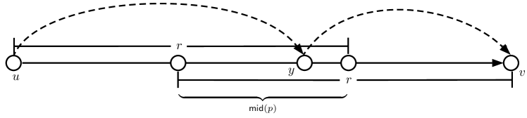
Figure 1: Example of a path $p=uv\diamond f$. If we can find a vertex $y\in\mathsf{mid}(p)$, then we can use $\mathcal{D}$ to compute $\|uy\diamond f\|$ and $\|yv\diamond f\|$, thus to compute the length of $p$.

Fix a large enough constant $C$, the preprocessing algorithm of $\mathrm{Extend}(\mathcal{D})$ is as follows: We preprocess $\mathcal{D}$, and then randomly sample a set $H$ of vertices, where every vertex $v\in V$ is in $H$ with probability $\min\{1,3CM\ln n/r\}$ independently. We have $|H|=\tilde{O}(nM/r)$ w.h.p.

Fix $u,v\in V$ and $f\in(V\cup E)$, suppose $p=uv\diamond f$ and $r\leq\|p\|<(3/2)r$. Then the probability that $H$ hits $\mathsf{mid}(p)$ (i.e. $H\cap\mathsf{mid}(p)\neq\varnothing$) is at least

$$1-(1-3CM\ln n/r)^{r/3M}\geq 1-1/n^{C}.$$

By a union bound over $O(n^{4})$ paths in $\mathcal{P}$, it follows that w.h.p. $H$ hits $\mathsf{mid}(p)$ for every path $p\in\mathcal{P}$.

The query algorithm for $\mathrm{Extend}(\mathcal{D})$ is as follows: Given a query $(u,v,f)$, if $\mathcal{D}(u,v,f)<r$, then we output $\mathcal{D}(u,v,f)$; otherwise we output

$$\min\left\{(3/2)r,\min_{h\in H,\mathcal{D}(u,h,f)<r,\mathcal{D}(h,v,f)<r}\left\{\mathcal{D}(u,h,f)+\mathcal{D}(h,v,f)\right\}\right\}.$$

It is easy to see that $\mathrm{Extend}(\mathcal{D})$ is a correct $(3/2)r$-truncated DSO, has preprocessing time $P+O(n^{2})$ and query time $\tilde{O}(nM/r)$.

2.4 Putting It Together

Let $a\in[0,1]$ be a constant that we pick later, and $r=n^{a}$. We first compute the APSP data using Theorem 1.3, which costs $\tilde{O}(n^{(3+\omega)/2}M^{1/2})$ time and will not be the bottleneck. Then we invoke Section 2.1 to build an $r$-truncated DSO $\mathcal{D}^{0}$ for $r=n^{a}$, which costs $\tilde{O}(r^{2}M\cdot\mathsf{MM}(n,n/r,n))$ time for directed graphs or $\tilde{O}(r\cdot Mn^{\omega})$ for undirected graphs. Then for every $1\leq i\leq\lceil\log_{3/2}(Mn/r)\rceil$, suppose we have an $r(3/2)^{i-1}$-truncated DSO $\mathcal{D}^{i-1}$, we can construct $\mathcal{D}^{i}=\mathrm{Fast}(\mathrm{Extend}(\mathcal{D}^{i-1}))$ which is an $r(3/2)^{i}$-truncated DSO. This step costs $\tilde{O}(n^{3}M/(r(3/2)^{i}))$ time. The preprocessing algorithm terminates when $i=i_{\star}=\lceil\log_{3/2}(Mn/r)\rceil=O(\log n)$, and we obtain an $r(3/2)^{i_{\star}}$-truncated DSO which is a (normal) DSO.

Case 1: the input graph is undirected.

The total preprocessing time is

$$\tilde{O}\left(r\cdot Mn^{\omega}+n^{3}M/r\right)=\tilde{O}\left(n^{\max\{\omega+a,3-a\}}M\right).$$

When $a=(3-\omega)/2$, this time complexity is $\tilde{O}(n^{(3+\omega)/2}M)=\tilde{O}(n^{2.6865}M)$.

Therefore, given an undirected graph $G=(V,E)$, there is a DSO with $\tilde{O}(n^{2.6865}M)$ preprocessing time and $O(1)$ query time.

Case 2: the input graph is directed.

The total preprocessing time is

$$\tilde{O}\left(r^{2}M\cdot\mathsf{MM}(n,n/r,n)+n^{3}M/r\right)=\tilde{O}\left(n^{2a+\omega(1-a)}M+n^{3-a}M\right).$$

(Recall that $\omega(1-a)$ is the exponent of multiplying an $n\times n^{1-a}$ matrix and an $n^{1-a}\times n$ matrix.)

Let $a=0.276724$, then $1-a=0.723276$. By convexity of the function $\omega(\cdot)$ [16], we have

$$\omega(1-a)\leq\frac{(a-0.25)\omega(0.7)+(0.3-a)\omega(0.75)}{0.75-0.7}.$$

We substitute $\omega(0.7)\leq 2.154399$ and $\omega(0.75)\leq 2.187543$ [12], and obtain:

$$\omega(1-a)\leq 20\cdot\left((a-0.25)\cdot 2.154399+(0.3-a)\cdot 2.187543\right)\leq 2.169829.$$

Therefore, given a directed graph $G=(V,E)$, there is a DSO with

$$\tilde{O}\left(n^{\max\{2a+\omega(1-a),3-a\}}M\right)=\tilde{O}(n^{2.723277}M)$$

preprocessing time and $O(1)$ query time.

3 Proof of 2.1 and Section 1.1

In this section, we prove 2.1. Note that Section 1.1 follows from 2.1 by setting $r=+\infty$.

See 2.1

3.1 The Preprocessing Algorithm

We review and slightly modify the preprocessing algorithm of [3]. For convenience, we denote $\|p\|_{r}=\min\{\|p\|,r\}$ for any path $p$ and number $r$.

Assigning priorities.

We assign each vertex a priority, which is independently sampled from the following distribution: for any positive integer $c$, each vertex has priority $c$ w.p. $1/2^{c}$. Denote $c(v)$ the priority of the vertex $v$. With high probability, all of the following are true:

• The maximum priority is $O(\log n)$.

• For every $c\leq O(\log n)$, there are $\tilde{O}(n/2^{c})$ vertices with priority $c$.

• Let $C$ be a large enough constant. For every shortest path $uv$ with at least $C\cdot 2^{c}\log n$ edges, there is a vertex on $uv$ whose priority is greater than $c$.

In the following discussions, we will assume that all of the above assumptions hold.

Fix a pair $u,v\in V$, let $s_{i}$ be the first vertex in $uv$ with priority $\geq i$, and $t_{i}$ be the last such vertex. Then we can write the path $uv$ as

$$u\rightsquigarrow s_{1}\rightsquigarrow s_{2}\rightsquigarrow\dots\rightsquigarrow s_{O(\log n)}\rightsquigarrow t_{O(\log n)}\rightsquigarrow\dots\rightsquigarrow t_{1}\rightsquigarrow v.$$

We say that the vertices $u,v,s_{i},t_{i}$ are key vertices, and the $i$-th key vertex is denoted as $k_{i}$. Then the path $uv$ can also be written as

$$u=k_{0}\rightsquigarrow k_{1}\rightsquigarrow\dots\rightsquigarrow k_{O(\log n)}=v.$$

It is important to see that

$$|k_{i}k_{i+1}|\leq C\cdot 2^{\min\{c(k_{i}),c(k_{i+1})\}}\log n$$ (1)

for every valid $i$, as otherwise there will be another key vertex between $k_{i}$ and $k_{i+1}$.

Data structures for quick location.

Suppose we are given a query $(u,v,f)$, the first thing we should do is to “locate” $f$, i.e. find the key vertices $k_{i},k_{i+1}\in uv$ such that $f\in k_{i}k_{i+1}$. We will utilize the following data (see also [2]).

• $\mathsf{CL}[u,v,c]$ (for “center left”): the first vertex in $uv$ with priority at least $c$;

• $\mathsf{CR}[u,v,c]$ (for “center right”): the last vertex in $uv$ with priority at least $c$; and

• $\mathsf{BCP}[u,v]$ (for “biggest center priority”): the maximum priority of any vertex on $uv$.

It is easy to compute these data in $\tilde{O}(n^{2})$ time: for every $u\in V$, we perform a depth-first search on the outgoing shortest path tree $T^{\sf out}(u)$ to compute $\mathsf{BCP}[u,\cdot]$; for every $u\in V$ and each priority $c$, we also perform a depth-first search on $T^{\sf out}(u)$ to compute $\mathsf{CL}[u,\cdot,c]$ and $\mathsf{CR}[u,\cdot,c]$.

In addition, for every $u,v\in V$, we store the key vertices on $uv$ into a hash table of size $O(\log n)$. Given a (vertex) failure $f$, we can output whether $f$ is among these key vertices on $uv$ in $O(1)$ worst-case time [10].

Data structures for avoiding a failure.

We use $\mathcal{D}$ to preprocess the input graph. Then we compute the following data:

1. For every $u,v\in V$, and every $1\leq i\leq\min\{C\cdot 2^{c(u)}\log n,|uv|\}$, let $x_{i}$ be the $i$-th vertex in the path $uv$. (Here $u$ is the $0$-th vertex.) We compute and store the value $\|uv\diamond x_{i}\|_{r}$. Also, let $e_{i}$ be the edge from $x_{i-1}$ to $x_{i}$, we compute and store $\|uv\diamond e_{i}\|_{r}$. Symmetrically, let $x_{-i}$ be the last $i$-th vertex in the path $vu$ (not $uv$!), and $e_{-i}$ be the edge from $x_{-i}$ to $x_{-(i-1)}$. For every $1\leq i\leq\min\{C\cdot 2^{c(u)}\log n,|vu|\}$, we compute and store $\|vu\diamond x_{-i}\|_{r}$ and $\|vu\diamond e_{-i}\|_{r}$.

2. For every $u,v\in V$ and consecutive key vertices $k_{i},k_{i+1}\in uv$ such that $k_{i}\neq u$ and $k_{i+1}\neq v$, let $y$ be the vertex in the portion $k_{i}\rightsquigarrow k_{i+1}$ that maximizes $\|uv\diamond y\|_{r}$. We compute and store $\|uv\diamond y\|_{r}$.

3. For every $u,v\in V$ and key vertex $k_{i}\in uv$, we compute and store $\|uv\diamond k_{i}\|_{r}$.

For each priority $c\leq\tilde{O}(1)$, there are $\tilde{O}(n/2^{c})$ vertices $u$ whose priority is exactly $c$. In (Data a), we make $\tilde{O}(n2^{c})$ queries for each such $u$ ($\tilde{O}(2^{c})$ queries for each $v\in V$). Therefore in total, we make $\tilde{O}(n^{2})$ queries in (Data a). We will show in Section 3.3 that we can compute (Data b) using $\tilde{O}(n^{2})$ queries to $\mathcal{D}$ and $\tilde{O}(n^{2})$ additional time. (Data c) can be computed in $\tilde{O}(n^{2})$ queries easily.

3.2 The Query Algorithm

Let $(u,v,f)$ be a query. We first check whether $f\in uv$ in the shortest path trees; if $f\not\in uv$, then it is easy to see that $\|uv\diamond f\|_{r}=\|uv\|_{r}$.

If $f$ is a vertex failure, we check whether $f$ is a key vertex on $uv$ (that is, $f=k_{i}$ for some $i$), using the hash tables. If this is the case, we return $\|uv\diamond f\|_{r}$ stored in (Data c) immediately.

Otherwise, we start by finding two consecutive key vertices $k_{i},k_{i+1}\in uv$ such that $f\in k_{i}k_{i+1}$. Recall that, if $\ell$ is the biggest priority of any vertex on $uv$, then the key vertices on $uv$ are

$$(u=){\sf CL}[u,v,1]\rightsquigarrow{\sf CL}[u,v,2]\rightsquigarrow\dots\rightsquigarrow{\sf CL}[u,v,\ell]\rightsquigarrow{\sf CR}[u,v,\ell]\rightsquigarrow\dots\rightsquigarrow{\sf CR}[u,v,2]\rightsquigarrow{\sf CR}[u,v,1](=v).$$

Denote $a$ and $b$ as the “tail” and “head” of $f$ respectively. In particular, if $f$ is a vertex failure then $a=b=f$; if $f$ is an edge failure then it is an edge from $a$ to $b$. We can find $k_{i}$ in $O(1)$ time using the following procedure:

• If $\mathsf{BCP}[b,v]=\ell$, then $f$ is in the range $(u,\mathsf{CR}[u,v,\ell])$, so we have $k_{i}=\mathsf{CL}[u,v,\mathsf{BCP}[u,a]]$.

• Otherwise, $f$ is in the range $(\mathsf{CR}[u,v,\ell],v)$ and we can see that $k_{i}=\mathsf{CR}[u,v,\mathsf{BCP}[b,v]+1]$.

We can find $k_{i+1}$ similarly. By Eq. (1), if $k_{i}=u$, then $|ub|\leq C\cdot 2^{c(u)}\log n$, and we can look up the value $\|uv\diamond f\|_{r}$ from (Data a) directly. Similarly, if $k_{i+1}=v$ then we can also look up $\|uv\diamond f\|_{r}$ from (Data a).

Now we assume that $k_{i}\neq u$ and $k_{i+1}\neq v$. A crucial observation is that

$$\|uv\diamond f\|=\min\{\|uk_{i+1}\diamond f\|+\|k_{i+1}v\|,\|uk_{i}\|+\|k_{i}v\diamond f\|,\|uv\diamond y\|\},$$ (2)

where $y$ is the vertex in $[k_{i},k_{i+1}]$ that maximizes $\|uv\diamond y\|$. The proof of Eq. (2) is as follows:

1. If $uv\diamond f$ goes through $k_{i}$, then $\|uv\diamond f\|=\|uk_{i}\|+\|k_{i}v\diamond f\|$.

2. If $uv\diamond f$ goes through $k_{i+1}$, then $\|uv\diamond f\|=\|uk_{i+1}\diamond f\|+\|k_{i+1}v\|$.

3. If $uv\diamond f$ goes through neither $k_{i}$ nor $k_{i+1}$, then it avoids the entire portion of $k_{i}\rightsquigarrow k_{i+1}$, thus also avoids $y$. We have $\|uv\diamond f\|\geq\|uv\diamond y\|$. But $\|uv\diamond y\|\geq\|uv\diamond a\|$ by definition of $y$, and $\|uv\diamond a\|\geq\|uv\diamond f\|$. (Recall that $a$ is the “tail” of $f$.) Thus $\|uv\diamond f\|=\|uv\diamond y\|$.

It is easy to see that a similar equation holds for $r$-truncated DSOs:

$$\|uv\diamond f\|_{r}=\min\{\|uk_{i+1}\diamond f\|_{r}+\|k_{i+1}v\|,\|uk_{i}\|+\|k_{i}v\diamond f\|_{r},\|uv\diamond y\|_{r},r\},$$ (3)

where $y$ is any vertex in $[k_{i},k_{i+1}]$ that maximizes $\|uv\diamond y\|_{r}$.

Recall that we already know the values $\|uk_{i}\|$ and $\|k_{i+1}v\|$. To compute $\|uk_{i+1}\diamond f\|_{r}$, we note that if $f$ is the last $j$-th vertex or edge in $uk_{i+1}$, then $j\leq C\cdot 2^{c(k_{i+1})}\log n$. Therefore we can look up the value of $\|uk_{i+1}\diamond f\|_{r}$ from (Data a). Similarly we can look up $\|k_{i}v\diamond f\|_{r}$. Finally, we can look up $\|uv\diamond y\|_{r}$ from (Data b).

We can see that the query time is $O(1)$.

3.3 Computing (Data b)

We will use the following notation. Let $p$ be a path from $u$ to $v$ which is fixed in context, and $a,b$ be two vertices in $p$. We will say that $a<b$ if $|p[u,a]|<|p[u,b]|$, i.e. $a$ appears strictly before $b$ on the path $p$. Similarly, $a>b$, $a\leq b$, $a\geq b$ mean $|p[u,a]|>|p[u,b]|$, $|p[u,a]|\leq|p[u,b]|$, $|p[u,a]|\geq|p[u,b]|$ respectively.

Let $u,v\in V$, and $s,t$ be two vertices on the path $uv$ such that $u<s<t<v$. Let $y\in[s,t]$ be the vertex in $[s,t]$ which maximizes $\|uv\diamond y\|_{r}$. We first show that assuming we have built some oracles, we can find this vertex $y$ in $O(\log n)$ oracle calls and $O(\log n)$ additional time. The idea is to use a binary search described in [3, Section 6].

Lemma 3.1.

Let $r$ be an integer, $u,v\in V$, and $s,t$ be two vertices on the path $uv$ such that $u<s<t<v$. Suppose we have the following oracles, each with $O(1)$ query time:

• an oracle that given a vertex $x\in st$, outputs $\|ut\diamond x\|_{r}$;

• an oracle that given a vertex $x\in st$, outputs $\|sv\diamond x\|_{r}$;

• an oracle that given an interval $[s^{\prime},t^{\prime}]$ such that $s\leq s^{\prime}\leq t^{\prime}\leq t$, outputs a vertex $x\in[s^{\prime},t^{\prime}]$ that maximizes the value $\|ut\diamond x\|_{r}$.

Then we can find a vertex $y\in[s,t]$ which maximizes $\|uv\diamond y\|_{r}$ in $O(\log n)$ time.

Proof 3.2.

For any $y\in[s,t]$, we denote

$$h(y)=\min\{\|ut\diamond y\|_{r}+\|tv\|,\|us\|+\|sv\diamond y\|_{r},r\}.$$

By Eq. (3), we have $\|uv\diamond y\|_{r}=\min\{h(y),\|uv\diamond y^{\star}\|_{r}\}$ where $y^{\star}$ is some vertex independent of $y$. Thus it suffices to find some $y\in[s,t]$ that maximizes $h(y)$.

We use a binary search. Assume that we know the optimal $y$ is in some interval $[s^{\prime},t^{\prime}]$, where $s\leq s^{\prime}<t^{\prime}\leq t$. (Initially we set $s^{\prime}=s$ and $t^{\prime}=t$.) If $|s^{\prime}t^{\prime}|=O(1)$ then we can use brute force to find a vertex $y\in[s^{\prime},t^{\prime}]$ that maximizes $h(y)$. Otherwise let $q$ be the middle point of $[s^{\prime},t^{\prime}]$, and we use the third oracle to find a vertex $y\in[s^{\prime},q]$ that maximizes $\|ut\diamond y\|_{r}$. There are two cases:

• If $\min\{\|ut\diamond y\|_{r}+\|tv\|,r\}=h(y)$, then we can restrict our attention to the interval $[q,t^{\prime}]$. This is because for every vertex $x\in[s^{\prime},q]$,

  $$h(x)\leq\min\{\|ut\diamond x\|_{r}+\|tv\|,r\}\leq\min\{\|ut\diamond y\|_{r}+\|tv\|,r\}=h(y).$$

• Otherwise, $h(y)=\|us\|+\|sv\diamond y\|_{r}$. Since $\|ut\diamond y\|_{r}+\|tv\|$ is strictly larger than $h(y)$, we know that $uv\diamond y$ does not go through $t$. Therefore $sv\diamond y$ avoids every vertex in $[q,t^{\prime}]$. (See Figure 2.) For every vertex $x\in[q,t^{\prime}]$,

  $$h(x)\leq\|us\|+\|sv\diamond x\|_{r}\leq\|us\|+\|sv\diamond y\|_{r}=h(y).$$

  It follows that we can restrict our attention to the interval $[s^{\prime},q]$ now.

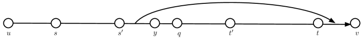
Figure 2: If $sv\diamond y$ does not go through $t$, then $sv\diamond y$ does not go through the whole interval $[q,t^{\prime}]$.

Therefore, we can always shrink the length of our candidate interval $[s^{\prime},t^{\prime}]$ by a half. It follows that we can find the desired vertex $y$ in $O(\log n)$ time.

Now we show how to compute (Data b) in $\tilde{O}(n^{2})$ time (assuming that (Data a) is ready). The most crucial ingredient is the following Range Maximum Query (RMQ) structures (used in the third item of Lemma 3.1).

For every $u,v\in V$, consider the following sequence (of length $\ell=\min\{|uv|-1,C\cdot 2^{c(v)}\log n\}$):

$$\left(\|uv\diamond x_{-1}\|_{r},\|uv\diamond x_{-2}\|_{r},\dots,\|uv\diamond x_{-\ell}\|_{r}\right),$$

where $x_{-i}$ denotes the last $i$-th vertex in the path $uv$ ($v$ is the last $0$-th). We build an RMQ structure of this sequence, which given a query $(s,t)$ ($1\leq s\leq t\leq\ell$), outputs a number $i\in[s,t]$ that maximizes $\|uv\diamond x_{-i}\|_{r}$. After we compute the above sequence, this data structure can be preprocessed in $O(\ell)$ time, and each query costs $O(1)$ time [1].

For every priority $c\leq O(\log n)$, there are $\tilde{O}(n/2^{c})$ vertices $v$ of this priority, and for each vertex $v$ we construct $n$ RMQ structures (one for each $u\in V$) on length-$\tilde{O}(2^{c})$ sequences. The total size of these RMQ structures is

$$\sum_{c=1}^{O(\log n)}\tilde{O}(n/2^{c})\cdot n\cdot\tilde{O}(2^{c})=\tilde{O}(n^{2}).$$

Therefore, these RMQ structures can be preprocessed in $\tilde{O}(n^{2})$ time. (Note that every element $\|uv\diamond x_{-i}\|_{r}$ is already computed in (Data a).)

To compute (Data b), we enumerate $u,v,k_{i},k_{i+1}$ where $k_{i},k_{i+1}$ are consecutive key vertices in $uv$. There are $\tilde{O}(n^{2})$ possible combinations of $(u,v,k_{i},k_{i+1})$. As argued in Section 3.2, we know that the following data are already computed in (Data a):

• $\|uk_{i+1}\diamond x\|_{r}$, for any $x\in k_{i}k_{i+1}$;

• $\|k_{i}v\diamond x\|_{r}$, for any $x\in k_{i}k_{i+1}$.

We also have the following RMQ oracles constructed above:

• An oracle that given any interval $[s^{\prime},t^{\prime}]$ on the path $uv$ such that $k_{i}\leq s^{\prime}\leq t^{\prime}\leq k_{i+1}$, finds the vertex $y\in[s^{\prime},t^{\prime}]$ that maximizes $\|uk_{i+1}\diamond y\|_{r}$ in $O(1)$ time.

It follows from Lemma 3.1 that we can find a vertex $y\in[k_{i},k_{i+1}]$ that maximizes $\|uv\diamond y\|_{r}$ in $O(\log n)$ time. The total time for computing (Data b) is thus $\tilde{O}(n^{2})$.

4 Reporting the Actual Path

In this section, we modify our DSO so that it also supports path-reporting queries: Given a query $(u,v,f)$, we want to report not only $\|uv\diamond f\|$, but also an actual shortest path from $u$ to $v$ that avoids $f$. If the path has length $\ell$, then the query algorithm runs in $O(\ell)$ time. Unfortunately, the size of the new DSO becomes $\tilde{O}(n^{2+a})$ where $a$ is the constant fixed in Section 2.4, i.e. $a=(3-\omega)/2$ for undirected graphs and $a=0.276724$ for directed graphs.

Recall that our DSO is constructed as follows. Fix $r=n^{a}$ and $i_{\star}=\lceil\log_{3/2}(Mn/r)\rceil$. Let $\mathcal{D}^{0}$ be an $r$-truncated DSO as in Section 2.1, and $\mathcal{D}^{i}=\mathrm{Fast}(\mathrm{Extend}(\mathcal{D}^{i-1}))$ for every $1\leq i\leq i_{\star}$. Then $\mathcal{D}^{i_{\star}}$ is a (normal) DSO.

Path-reporting structure for $\mathcal{D}^{0}$.

Recall that the structure $\mathcal{D}^{0}$ consists of subgraphs $G_{i}^{\mathsf{e}}$ and $G_{i}^{\mathsf{v}}$. For each subgraph, we can compute an implicit representation of the shortest paths of length at most $r$ as follows:

• If the graph is directed, we run the first $\lceil\log_{3/2}r\rceil$ iterations of the algorithm rand-short-path in [22]. After that, the matrix $W$ in [22, Figure 2] encodes shortest paths of length at most $r$.

• If the graph is undirected, we simply use [19, Section 4].

Given the implicit representations, it is easy to report the actual path for any query of $\mathcal{D}^{0}$. As we need to store $\tilde{O}(r)$ such representations, the size of our DSO becomes $\tilde{O}(n^{2}r)$.

Path-reporting algorithm for $\mathcal{D}^{i}$.

For every $1\leq i\leq i_{\star}$, the preprocessing algorithm of $\mathcal{D}^{i}$ invokes $\tilde{O}(n^{2})$ queries to $\mathrm{Extend}(\mathcal{D}^{i-1})$. For each such query $(u_{q},v_{q},f_{q})$:

• If $\|u_{q}v_{q}\diamond f_{q}\|\leq r$, then the path $u_{q}v_{q}\diamond f_{q}$ can be retrieved from $\mathcal{D}^{0}$, thus we do not need to store anything.

• Otherwise, suppose $i_{q}=\lfloor\log_{3/2}(\|u_{q}v_{q}\diamond f_{q}\|/r)\rfloor$, then $r(3/2)^{i_{q}}\leq\|u_{q}v_{q}\diamond f_{q}\|<r(3/2)^{i_{q}+1}$. If $i_{q}\geq i$, then $\mathcal{D}^{i}$ do not need the exact value of $\|u_{q}v_{q}\diamond f_{q}\|$; therefore we may assume $i_{q}<i$. This means that the query $(u_{q},v_{q},f_{q})$ is captured by $\mathcal{D}^{i_{q}+1}$ but not by $\mathcal{D}^{i_{q}}$. We store the “hitting vertex” $h_{q}$ in $\mathrm{Extend}(\mathcal{D}^{i_{q}})$ that hits $\mathsf{mid}(u_{q}v_{q}\diamond f_{q})$ (as in Section 2.3). Then, $u_{q}v_{q}\diamond f_{q}$ is the concatenation of $u_{q}h_{q}\diamond f_{q}$ and $h_{q}v_{q}\diamond f_{q}$, both of which can be retrieved from $\mathcal{D}^{i_{q}}$.

Consider a query $(u,v,f)$. By the query algorithm in Section 3.2, $uv\diamond f$ belongs to one of the following cases:

1. the concatenation of $uk$ and $kv\diamond f$, for some key vertex $k$;

2. the concatenation of $uk\diamond f$ and $kv$, for some key vertex $k$;

3. $uv\diamond y$ for the vertex $y$ computed in Section 3.3.

In all of these cases, $uv\diamond f$ is the concatenation of a shortest path in $G$ (that is, $uk$, $kv$, or the empty path) and some $u_{q}v_{q}\diamond f_{q}$, where $(u_{q},v_{q},f_{q})$ is a query recorded in the preprocessing algorithm.

• We can retrieve the shortest path in $G$ using the shortest path trees.

• If $\|u_{q}v_{q}\diamond f_{q}\|\leq r$, we can retrieve it in $\mathcal{D}^{0}$; otherwise we recursively find $u_{q}h_{q}\diamond f_{q}$ and $h_{q}v_{q}\diamond f_{q}$ in $\mathcal{D}^{i_{q}}$, and concatenate them together to form $u_{q}v_{q}\diamond f_{q}$.

Time complexity.

It remains to show that only $O(\ell)$ time is spent on retrieving a path of length $\ell$. The time complexity is proportional to $\ell$ plus the number of preprocessed queries $(u_{q},v_{q},f_{q})$ that we access (over all DSOs $\mathcal{D}^{i}$). Note that each $(u_{q},v_{q},f_{q})$ corresponds to a hitting vertex $h_{q}$ on the reported path, and different queries correspond to different $h_{q}$’s. Therefore the number of such queries is at most $\ell$, which means the path-reporting algorithm only takes $O(\ell)$ time.

5 Open Questions

The main open problem after this work is to improve the preprocessing time for DSOs. Can we improve the preprocessing time for directed graphs to $\tilde{O}(n^{2.5286}M)$, matching the current best algorithm for APSP in directed graphs [22]? A subsequent work by Yong Gu and the author [14] improved the preprocessing time to $\tilde{O}(n^{2.5794}M)$, but there is still a gap between this time bound and the time bound for APSP.

We can compute APSP for undirected graphs in $\tilde{O}(n^{\omega}M)$ time [18, 19], and another interesting question is whether there is a DSO for undirected graphs with the same preprocessing time (and constant query time).

Finally, can we extend our technique to deal with negative weights? There are a few candidate definitions of “$r$-truncated DSOs” in this case, if we interpret $r$ as the number of edges in the shortest path, instead of the length of the shortest path. For example, we may define a DSO is $r$-truncated if on a query $(u,v,f)$, it outputs some value no less than $\|uv\diamond f\|$, and when $|uv\diamond f|\leq r$, it outputs $\|uv\diamond f\|$ exactly. However, it seems that every definition of “$r$-truncated DSO” that we tried were not compatible with arguments in Section 3.3.

Appendix A Breaking Ties for Non-unique Shortest Paths

In this section, we prove Theorem 1.2 and 1.3.

Recall that in a subgraph $G^{\prime}$ of $G$, we denote $w_{G^{\prime}}(u,v)$ as the largest (w.r.t. $\prec$) edge $w$ such that there is a shortest path from $u$ to $v$ whose bottleneck edge (i.e. smallest w.r.t. $\prec$) is $w$. Also the path $\rho_{G^{\prime}}(u,v)$ is defined, inductively from the smallest $\|uv\|$ to the largest $\|uv\|$, as follows: If $u=v$, then $\rho_{G^{\prime}}(u,v)$ is the empty path; otherwise, suppose $w_{G^{\prime}}(u,v)$ is an edge from $u^{\star}$ to $v^{\star}$, then $\rho_{G^{\prime}}(u,v)$ is the concatenation of $\rho_{G^{\prime}}(u,u^{\star})$, $w_{G^{\prime}}(u,v)$ and $\rho_{G^{\prime}}(v^{\star},v)$.

See 1.2

Proof A.1.

In this proof we will always use the following notation: Let $w=w_{G^{\prime}}(u,v)$, and suppose $w$ is an edge from $u^{\star}$ to $v^{\star}$. Denote $p_{1}=\rho_{G^{\prime}}(u,u^{\star})$ and $p_{2}=\rho_{G^{\prime}}(v^{\star},v)$. We will prove Theorem 1.2 inductively, from the smallest $\|uv\|$ to the largest $\|uv\|$. Theorem 1.2 is clearly true when $u=v$.

(Property a): If both $u^{\prime},v^{\prime}\in p_{1}$, then (Property a) is true by induction on $p_{1}$. Similarly, if both $u^{\prime},v^{\prime}\in p_{2}$, then (Property a) is also true by induction on $p_{2}$.

Now suppose $u^{\prime}\in p_{1}$ and $v^{\prime}\in p_{2}$. Our first observation is that $w_{G^{\prime}}(u^{\prime},v^{\prime})=w_{G^{\prime}}(u,v)=w$. Actually, since $(\rho_{G^{\prime}}(u,v))[u^{\prime},v^{\prime}]$ is a shortest path from $u^{\prime}$ to $v^{\prime}$ with bottleneck edge $w$, we have $w_{G^{\prime}}(u^{\prime},v^{\prime})\succeq w$. But if there is any shortest path $p^{\prime}$ from $u^{\prime}$ to $v^{\prime}$ whose bottleneck edge is $\succ w$, the concatenation of $p_{1}[u,u^{\prime}]$, $p^{\prime}$ and $p_{2}[v^{\prime},v]$ will be a shortest path from $u$ to $v$ with bottleneck edge $\succ w$, a contradiction. Thus we can only have $w_{G^{\prime}}(u^{\prime},v^{\prime})=w$.

By induction on $p_{1}$, we have $\rho_{G^{\prime}}(u^{\prime},u^{\star})=p_{1}[u^{\prime},u^{\star}]$. By induction on $p_{2}$, we have $\rho_{G^{\prime}}(v^{\star},v)=p_{2}[v^{\star},v]$. Therefore, $\rho_{G^{\prime}}(u^{\prime},v^{\prime})$ is the concatenation of $p_{1}[u^{\prime},u^{\star}]$, $w$, and $p_{2}[v^{\star},v]$. This path coincides with the $u^{\prime}\rightsquigarrow v^{\prime}$ portion of $\rho_{G^{\prime}}(u,v)$.

(Property b): it suffices to prove $w_{G}(u,v)=w_{G^{\prime}}(u,v)$, and use induction on $p_{1}$ and $p_{2}$. Since $G^{\prime}$ is a subgraph of $G$, and the distance from $u$ to $v$ is the same in $G$ and $G^{\prime}$, we have $w_{G}(u,v)\succeq w_{G^{\prime}}(u,v)$. Since $\rho_{G}(u,v)$ is completely in $G^{\prime}$ and the bottleneck edge of $\rho_{G}(u,v)$ is $w_{G}(u,v)$, we have $w_{G^{\prime}}(u,v)\succeq w_{G}(u,v)$. This completes the proof.

See 1.3

Proof A.2 (Proof Sketch).

The first step is to compute $w_{G^{\prime}}(u,v)$ for every pair of vertices $u,v\in V$. This problem is exactly the same as the all-pairs bottleneck shortest paths problem (APBSP; [8, Theorem 4.4]). However, Theorem 4.4 of [8] only claims to work for unweighted graphs, so we verify that it also works for graphs with positive integer edge weights here.

We start by using [22] to compute $\|\rho_{G^{\prime}}(u,v)\|$ for every $u,v\in V$. Then, for every $0\leq i\leq\lceil\log_{3/2}(nM)\rceil$ and $r=(3/2)^{i}$, assuming we have computed $w_{G^{\prime}}(u,v)$ for every $u,v$ such that $\|\rho_{G^{\prime}}(u,v)\|\leq r$, we compute $w_{G^{\prime}}(u,v)$ for every $u,v$ such that $\|\rho_{G^{\prime}}(u,v)\|\leq(3/2)r$. This is done as follows. We sample a vertex set $H$ by adding each vertex into $H$ independently w.p. $\Theta(M\log n/r)$, then w.h.p. $H$ hits $\mathsf{mid}(\rho_{G^{\prime}}(u,v))$ for every $u,v$ such that $r<\|\rho_{G^{\prime}}(u,v)\|\leq(3/2)r$. (Recall that $\mathsf{mid}(\rho_{G^{\prime}}(u,v))$ is the “middle $1/3$ part” of $\rho_{G^{\prime}}(u,v)$.) Let $D,W$ be $V\times H$ matrices such that for every $u\in V,h\in H$,

• if $\|\rho_{G^{\prime}}(u,h)\|\leq r$, then $D[u,h]=\|\rho_{G^{\prime}}(u,h)\|$ and $W[u,h]=w_{G^{\prime}}(u,h)$;

• otherwise $D[u,h]=+\infty$ and $W[u,h]=-\infty$.

Then we compute the Distance-Max-Min product (Definition 4.3 of [8]) of $(D,W)$ and $(D^{\sf T},W^{\sf T})$ to obtain a $V\times V$ matrix $W^{\prime}$ such that

$$W^{\prime}[u,v]=\max_{h:D[u,h]+D[h,v]=\|\rho_{G^{\prime}}(u,v)\|}\left\{\min\left\{W[u,h],W[h,v]\right\}\right\}.$$

We can see that $W^{\prime}[u,v]=w_{G^{\prime}}(u,v)$ for every $u,v\in V$ such that $r<\|\rho_{G^{\prime}}(u,v)\|\leq(3/2)r$. This completes the description of the APBSP algorithm.

Now we analyze the time complexity. Let $|H|=n^{s}$, then $r=\tilde{O}(n^{1-s}M)$, and the finite entries in $D$ are in $\{1,2,\dots,r\}$. By [8, Theorem 4.3], the Distance-Max-Min product takes

$$O\left(\min\left\{n^{2+s},r^{1/2}n^{1+s/2+\omega(s)/2}\right\}\right)=\tilde{O}\left(\min\left\{n^{2+s},n^{(3+\omega(s))/2}M^{1/2}\right\}\right)\leq\tilde{O}\left(n^{(3+\omega)/2}M^{1/2}\right)$$

time. Since we only execute $O(\log n)$ rounds of Distance-Max-Min product, the overall running time of the algorithm is $\tilde{O}\left(n^{(3+\omega)/2}M^{1/2}\right)$.

Now we construct the outgoing shortest path trees from the table of $w_{G^{\prime}}(u,v)$ for every $u,v\in V$. It suffices to compute the parents of each node $v$ in the trees $T^{\sf out}(u)$ (which we denote as $\mathrm{parent}_{u}(v)$). We compute $\mathrm{parent}_{u}(v)$ inductively from the smallest $\|uv\|$ to the largest.

Let $(u,v)$ be the pair of vertices we are processing, and assume that for every $u^{\prime},v^{\prime}\in V$ such that $\|u^{\prime}v^{\prime}\|<\|uv\|$, we have already computed $\mathrm{parent}_{u^{\prime}}(v^{\prime})$. Suppose $w_{G^{\prime}}(u,v)$ is an edge from $u^{\star}$ to $v^{\star}$. If $v^{\star}=v$, then $\mathrm{parent}_{u}(v)=u^{\star}$. Otherwise, it is easy to see that $\|\rho_{G^{\prime}}(v^{\star},v)\|<\|\rho_{G^{\prime}}(u,v)\|$ and $\mathrm{parent}_{u}(v)=\mathrm{parent}_{v^{\star}}(v)$. Thus we can compute every outgoing shortest path tree in $\tilde{O}(n^{2})$ time. Similarly, the incoming shortest path trees can also be computed in $\tilde{O}(n^{2})$ time.

References

- [1] Michael A. Bender and Martin Farach-Colton. The LCA problem revisited. In Gaston H. Gonnet, Daniel Panario, and Alfredo Viola, editors, LATIN 2000: Theoretical Informatics, 4th Latin American Symposium, Punta del Este, Uruguay, April 10-14, 2000, Proceedings, volume 1776 of Lecture Notes in Computer Science, pages 88–94. Springer, 2000. URL: https://doi.org/10.1007/10719839_9.
- [2] Aaron Bernstein and David R. Karger. Improved distance sensitivity oracles via random sampling. In Shang-Hua Teng, editor, Proceedings of the Nineteenth Annual ACM-SIAM Symposium on Discrete Algorithms, SODA 2008, San Francisco, California, USA, January 20-22, 2008, pages 34–43. SIAM, 2008. URL: http://dl.acm.org/citation.cfm?id=1347082.1347087.
- [3] Aaron Bernstein and David R. Karger. A nearly optimal oracle for avoiding failed vertices and edges. In Michael Mitzenmacher, editor, Proceedings of the 41st Annual ACM Symposium on Theory of Computing, STOC 2009, Bethesda, MD, USA, May 31 - June 2, 2009, pages 101–110. ACM, 2009. URL: https://doi.org/10.1145/1536414.1536431.
- [4] Shiri Chechik and Sarel Cohen. Distance sensitivity oracles with subcubic preprocessing time and fast query time. In Konstantin Makarychev, Yury Makarychev, Madhur Tulsiani, Gautam Kamath, and Julia Chuzhoy, editors, Proccedings of the 52nd Annual ACM SIGACT Symposium on Theory of Computing, STOC 2020, Chicago, IL, USA, June 22-26, 2020, pages 1375–1388. ACM, 2020. URL: https://doi.org/10.1145/3357713.3384253.
- [5] Camil Demetrescu and Giuseppe F. Italiano. A new approach to dynamic all pairs shortest paths. J. ACM, 51(6):968–992, 2004. URL: https://doi.org/10.1145/1039488.1039492.
- [6] Camil Demetrescu, Mikkel Thorup, Rezaul Alam Chowdhury, and Vijaya Ramachandran. Oracles for distances avoiding a failed node or link. SIAM J. Comput., 37(5):1299–1318, 2008. URL: https://doi.org/10.1137/S0097539705429847.
- [7] Ran Duan and Seth Pettie. Dual-failure distance and connectivity oracles. In Claire Mathieu, editor, Proceedings of the Twentieth Annual ACM-SIAM Symposium on Discrete Algorithms, SODA 2009, New York, NY, USA, January 4-6, 2009, pages 506–515. SIAM, 2009. URL: http://dl.acm.org/citation.cfm?id=1496770.1496826.
- [8] Ran Duan and Seth Pettie. Fast algorithms for (max, min)-matrix multiplication and bottleneck shortest paths. In Claire Mathieu, editor, Proceedings of the Twentieth Annual ACM-SIAM Symposium on Discrete Algorithms, SODA 2009, New York, NY, USA, January 4-6, 2009, pages 384–391. SIAM, 2009. URL: http://dl.acm.org/citation.cfm?id=1496770.1496813.
- [9] Ran Duan and Tianyi Zhang. Improved distance sensitivity oracles via tree partitioning. In Faith Ellen, Antonina Kolokolova, and Jörg-Rüdiger Sack, editors, Algorithms and Data Structures - 15th International Symposium, WADS 2017, St. John’s, NL, Canada, July 31 - August 2, 2017, Proceedings, volume 10389 of Lecture Notes in Computer Science, pages 349–360. Springer, 2017. URL: https://doi.org/10.1007/978-3-319-62127-2_30.
- [10] Michael L. Fredman, János Komlós, and Endre Szemerédi. Storing a sparse table with worst case access time. In 23rd Annual Symposium on Foundations of Computer Science, Chicago, Illinois, USA, 3-5 November 1982, pages 165–169. IEEE Computer Society, 1982. URL: https://doi.org/10.1109/SFCS.1982.39.
- [11] François Le Gall. Powers of tensors and fast matrix multiplication. In Katsusuke Nabeshima, Kosaku Nagasaka, Franz Winkler, and Ágnes Szántó, editors, International Symposium on Symbolic and Algebraic Computation, ISSAC ’14, Kobe, Japan, July 23-25, 2014, pages 296–303. ACM, 2014. URL: https://doi.org/10.1145/2608628.2608664.
- [12] Francois Le Gall and Florent Urrutia. Improved rectangular matrix multiplication using powers of the Coppersmith-Winograd tensor. In Artur Czumaj, editor, Proceedings of the Twenty-Ninth Annual ACM-SIAM Symposium on Discrete Algorithms, SODA 2018, New Orleans, LA, USA, January 7-10, 2018, pages 1029–1046. SIAM, 2018. URL: https://doi.org/10.1137/1.9781611975031.67.
- [13] Fabrizio Grandoni and Virginia Vassilevska Williams. Faster replacement paths and distance sensitivity oracles. ACM Trans. Algorithms, 16(1):15:1–15:25, 2020. URL: https://doi.org/10.1145/3365835.
- [14] Yong Gu and Hanlin Ren. Constructing a distance sensitivity oracle in time. In 48th International Colloquium on Automata, Languages, and Programming, ICALP 2021, July 12-16, 2021, Glasgow, Scotland (Virtual Conference), volume 198 of LIPIcs, pages 76:1–76:20. Schloss Dagstuhl - Leibniz-Zentrum für Informatik, 2021. URL: https://doi.org/10.4230/LIPIcs.ICALP.2021.76.
- [15] Andrea Lincoln, Virginia Vassilevska Williams, and R. Ryan Williams. Tight hardness for shortest cycles and paths in sparse graphs. In Artur Czumaj, editor, Proceedings of the Twenty-Ninth Annual ACM-SIAM Symposium on Discrete Algorithms, SODA 2018, New Orleans, LA, USA, January 7-10, 2018, pages 1236–1252. SIAM, 2018. URL: https://doi.org/10.1137/1.9781611975031.80.
- [16] Grazia Lotti and Francesco Romani. On the asymptotic complexity of rectangular matrix multiplication. Theor. Comput. Sci., 23:171–185, 1983. URL: https://doi.org/10.1016/0304-3975(83)90054-3.
- [17] Ketan Mulmuley, Umesh V. Vazirani, and Vijay V. Vazirani. Matching is as easy as matrix inversion. Combinatorica, 7(1):105–113, 1987. URL: https://doi.org/10.1007/BF02579206.
- [18] Raimund Seidel. On the all-pairs-shortest-path problem in unweighted undirected graphs. J. Comput. Syst. Sci., 51(3):400–403, 1995. URL: https://doi.org/10.1006/jcss.1995.1078.
- [19] Avi Shoshan and Uri Zwick. All pairs shortest paths in undirected graphs with integer weights. In 40th Annual Symposium on Foundations of Computer Science, FOCS ’99, 17-18 October, 1999, New York, NY, USA, pages 605–615. IEEE Computer Society, 1999. URL: https://doi.org/10.1109/SFFCS.1999.814635.
- [20] Noam Ta-Shma. A simple proof of the isolation lemma. Electronic Colloquium on Computational Complexity (ECCC), 22:80, 2015. URL: https://eccc.weizmann.ac.il/report/2015/080.
- [21] Oren Weimann and Raphael Yuster. Replacement paths and distance sensitivity oracles via fast matrix multiplication. ACM Trans. Algorithms, 9(2):14:1–14:13, 2013. URL: https://doi.org/10.1145/2438645.2438646.
- [22] Uri Zwick. All pairs shortest paths using bridging sets and rectangular matrix multiplication. J. ACM, 49(3):289–317, 2002. URL: https://doi.org/10.1145/567112.567114.