Preconditioned Gradient Descent Algorithm for Inverse Filtering on Spatially Distributed Networks

Abstract

Graph filters and their inverses have been widely used in denoising, smoothing, sampling, interpolating and learning. Implementation of an inverse filtering procedure on spatially distributed networks (SDNs) is a remarkable challenge, as each agent on an SDN is equipped with a data processing subsystem with limited capacity and a communication subsystem with confined range due to engineering limitations. In this letter, we introduce a preconditioned gradient descent algorithm to implement the inverse filtering procedure associated with a graph filter having small geodesic-width. The proposed algorithm converges exponentially, and it can be implemented at vertex level and applied to time-varying inverse filtering on SDNs.

Keywords: Graph signal processing, Inverse filtering, Spatially distributed network, Gradient descent method, Preconditioning, Quasi-Newton method

I Introduction

Spatially distributed networks (SDNs) have been widely used in (wireless) sensor networks, drone fleets, smart grids and many real world applications [1]–[4]. An SDN has a large amount of agents and each agent equipped with a data processing subsystem having limited data storage and computation power and a communication subsystem for data exchanging to its “neighboring” agents within communication range. The topology of an SDN can be described by a connected, undirected and unweighted finite graph ${\mathcal{G}}:=(V,E)$ with a vertex in $V$ representing an agent and an edge in $E$ between vertices indicating that the corresponding agents are within some range in the spatial space. In this letter, we consider SDNs equipped with a communication subsystem at each agent to directly communicate between two agents if the geodesic distance between their corresponding vertices $i,j\in V$ is at most $L$,

$$\rho(i,j)\leq L,\vspace{-.5em}$$ (I.1)

where the geodesic distance $\rho(i,j)$ is the number of edges in a shortest path connecting $i,j\in V$, and we call the minimal integer $L\geq 1$ in (I.1) as the communication range of the SDN. Therefore the implementation of data processing on our SDNs is a distributed task and it should be designed at agent/vertex level with confined communication range. In this letter, we consider the implementation of graph filtering and inverse filtering on SDNs, which are required to be fulfilled at agent level with communication range no more than $L$.

A signal on a graph ${\mathcal{G}}=(V,E)$ is a vector ${\bf x}=(x(i))_{i\in V}$ indexed by the vertex set, and a graph filter ${\bf H}$ maps a graph signal ${\bf x}$ linearly to another graph signal ${\bf y}={\bf H}{\bf x}$, which is usually represented by a matrix ${\bf H}=(H(i,j))_{i,j\in V}$ indexed by vertices in $V$. Graph filtering ${\bf x}\mapsto{\bf Hx}$ and its inverse filtering ${\bf y}\mapsto{\bf H}^{-1}{\bf y}$ play important roles in graph signal processing and they have been used in smoothing, sampling, interpolating and many real-world applications [2], [5]–[9]. A graph filter ${\bf H}=(H(i,j))_{i,j\in V}$ is said to have geodesic-width $\omega({\bf H})$ if

$$H(i,j)=0\ \ {\rm for\ all}\ \ i,j\in V\ \ {\rm with}\ \ \rho(i,j)>\omega({\bf H})\vspace{-.5em}$$ (I.2)

[4, 10, 11]. For a filter ${\bf H}=(H(i,j))_{i,j\in V}$ with geodesic-width $\omega({\bf H})$, the corresponding filtering process

$$(x(i))_{i\in V}=:{\bf x}\longmapsto{\bf Hx}={\bf y}:=(y(i))_{i\in V}\vspace{-.5em}$$ (I.3)

can be implemented at vertex level, and the output at a vertex $i\in V$ is a “weighted” sum of the input in its $\omega({\bf H})$-neighborhood,

$$y(i)=\sum_{\rho(j,i)\leq\omega({\bf H})}H(i,j)x(j).\vspace{-.5em}$$ (I.4)

For SDNs with communication range $L\geq\omega({\bf H})$, the above implementation at vertex level provides an essential tool for the filtering procedure (I.3), in which each agent $i\in V$ has equipped with subsystems to store $H(i,j)$ and $x(j)$ with $\rho(j,i)\leq\omega({\bf H})$, to compute addition and multiplication in (I.4), and to exchange data to its neighboring agents $j\in V$ satisfying $\rho(j,i)\leq\omega({\bf H})$.

For an invertible filter ${\bf H}$, the implementation of the inverse filtering procedure

$${\bf y}\longmapsto{\bf H}^{-1}{\bf y}=:{\bf x}\vspace{-.3em}$$ (I.5)

cannot be directly applied for our SDNs, since the inverse filter ${\bf H}^{-1}$ may have geodesic-width larger than the communication range $L$. For the consideration of implementing inverse filtering on an SDN with communication range $L\geq 1$, we construct a diagonal preconditioning matrix ${\bf P}_{\bf H}$ in (II.1) at vertex level, and propose the preconditioned gradient descent algorithm (PGDA) (II.8) to implement inverse filtering on the SDN, see Algorithms II.1 and II.2.

A conventional approach to implement the inverse filtering procedure (I.5) is via the iterative quasi-Newton method

$${\bf e}^{(m)}={\bf H}{\bf x}^{(m-1)}-{\bf y}\ {\rm and}\ {\bf x}^{(m)}={\bf x}^{(m-1)}-{\bf G}{\bf e}^{(m)},\ m\geq 1,\vspace{-.3em}$$ (I.6)

with arbitrary initial ${\bf x}^{(0)}$, where the graph filter ${\bf G}$ is an approximation to the inverse ${\bf H}^{-1}$. A challenge in the quasi-Newton method is how to select the approximation filter ${\mathbf{G}}$ appropriately. For the widely used polynomial graph filters ${\bf H}=h({\bf S})=\sum_{k=0}^{K}h_{k}{\bf S}^{k}$ of a graph shift ${\bf S}$ where $h(t)=\sum_{k=0}^{K}h_{k}t^{k}$ [11]–[19], several methods have been proposed to construct polynomial approximation filters ${\bf G}$ [13, 14, 16, 17, 19]. However, for the convergence of the corresponding quasi-Newton method, some prior knowledge is required for the polynomial $h$ and the graph shift ${\bf S}$, such as the whole spectrum of the shift ${\bf S}$ in the optimal polynomial approximation method [19], the interval containing the spectrum of the shift ${\bf S}$ in the Chebyshev approximation method [16, 17, 19], and the spectral radius of the shift ${\bf S}$ and the zero set of the polynomial $h$ in the autoregressive moving average filtering algorithm [13, 14]. For a non-polynomial graph filter ${\bf H}$, the approximation filter in the gradient descent method is of the form ${\bf G}=\beta{\bf H}^{T}$ with selection of the optimal step length $\beta$ depending on maximal and minimal singular values of the filter ${\bf H}$ [12, 20], and the approximation filter in the iterative matrix inverse approximation algorithm (IMIA) could be selected under a strong assumption on ${\bf H}$ [10, Theorem 3.2]. The proposed PGDA (II.8) is the quasi-Newton method (I.6) with ${\bf P}_{\bf H}^{-2}{\bf H}^{T}$ being selected as the approximation filter ${\bf G}$, see (II.3). Comparing with the quasi-Newton methods in [10, 12, 13, 14, 16, 17, 19, 20], one significance of the proposed PGDA is that the sequence ${\bf x}^{(m)},m\geq 0$, in (II.8) converges exponentially to the output ${\bf x}$ of the inverse filtering procedure (I.5) whenever the filter ${\bf H}$ is invertible, see Theorems II.3 and III.1.

For a time-varying filter the quasi-Newton method (I.6) to implement their inverse filtering on SDNs should be self-adaptive as each agent does not have the whole time-varying filter and it only receives the submatrix of the filter within the communication range [4]. The IMIA algorithm is self-adaptive [10, Eq. (3.4)], and the gradient descent method [12, 20] is not self-adaptive in general except that the step length $\beta$ can be chosen to be time-independent. The second significance of the proposed PGDA is its self-adaptivity and compatibility to implement the time-varying inverse filtering procedure on our SDNs, as the preconditioner ${\bf P}_{\bf H}$ (and hence the approximation filter ${\bf P}_{\bf H}^{-2}{\bf H}^{T}$ in the PGDA) is constructed at vertex level with confined communication range, see Algorithm II.1.

II Preconditioned gradient descent algorithm for inverse filtering

Let ${\mathcal{G}}:=(V,E)$ be a connected, undirected and unweighted graph and ${\bf H}=(H(i,j))_{i,j\in V}$ be a filter on the graph ${\mathcal{G}}$ with geodesic-width $\omega({\bf H})$. In this section, we induce a diagonal matrix ${\bf P}_{\bf H}$ with diagonal elements $P_{\bf H}(i,i),i\in V$, given by

$$\hskip-5.78172pt{P}_{\bf H}(i,i):= \hskip-5.78172pt\max_{k\in B(i,\omega({\bf H}))}\Big{\{}\max\Big{(}\sum_{j\in B(k,\omega({\bf H}))}|H(j,k)|,$$ (II.1)

$$\qquad\qquad\quad\sum_{j\in B(k,\omega({\bf H}))}|H(k,j)|\Big{)}\Big{\}},\vspace{-.3em}$$

where we denote the set of all $s$-hop neighbors of a vertex $i\in V$ by $B(i,s)=\{j\in V,\ \rho(j,i)\leq s\},\ s\geq 0$. The above diagonal matrix ${\bf P}_{\bf H}$ can be evaluated at vertex level, and constructed on SDNs with communication range $L\geq\omega({\bf H})$, see Algorithm II.1.

Algorithm II.1 Realization of the preconditioner ${\bf P}_{\bf H}$ at a vertex $i\in V$.

  Inputs: Geodesic width $\omega({\bf H})$ of the filter ${\bf H}$ and nonzero entries $H(i,j)$ and $H(j,i)$ for $j\in B(i,\omega({\bf H}))$ in the $i$-th row and column of the filter ${\bf H}$.

  1) Calculate$d(i)=\max\Big{\{}\sum\limits_{j\in B(i,\omega({\bf H}))}|H(i,j)|,\sum\limits_{j\in B(i,\omega({\bf H}))}|H(j,i)|\Big{\}}$.

  2) Send $d(i)$ to all neighbors $k\in B(i,\omega({\bf H}))\backslash\{i\}$ and receive $d(k)$ from neighbors $k\in B(i,\omega({\bf H}))\backslash\{i\}$.

  3) Calculate $P_{\bf H}(i,i)=\max\limits_{k\in B(i,\omega({\bf H}))}d(k)$.

  Output: $P_{\bf H}(i,i)$.

For symmetric matrices ${\bf A}$ and ${\bf B}$, we use ${\bf B}\preceq{\bf A}$ and ${\bf B}\prec{\bf A}$ to denote the positive semidefiniteness and positive definiteness of their difference ${\bf A}-{\bf B}$ respectively. A crucial observation about the diagonal matrix $\bf P_{H}$ is as follows.

Theorem II.1.

Let ${\bf H}=(H(i,j))_{i,j\in V}$ be a graph filter with geodesic-width $\omega({\bf H})$ and ${\bf P}_{\bf H}$ be as in (II.1). Then

$${\bf H}^{T}{\bf H}\preceq{\bf P}_{\bf H}^{2}.\vspace{-.3em}$$ (II.2)

Proof.

For ${\bf x}=(x(i))_{i\in V}$, we have

$$0 \hskip-5.78172pt\leq \hskip-5.78172pt{\bf x}^{T}{\bf H}^{T}{\bf H}{\bf x}=\sum_{j\in V}\Big{|}\sum_{i\in V}H(j,i)x(i)\Big{|}^{2}$$

$$\hskip-5.78172pt\leq \hskip-5.78172pt\sum_{j\in V}\Big{(}\sum_{i\in V}|H(j,i)||x(i)|^{2}\Big{)}\times\Big{(}\sum_{i^{\prime}\in V}|H(j,i^{\prime})|\Big{)}$$

$$\hskip-5.78172pt= \hskip-5.78172pt\sum_{i\in V}|x(i)|^{2}\sum_{j\in B(i,\omega({\bf H}))}|H(j,i)|\times\Big{(}\sum_{i^{\prime}\in V}|H(j,i^{\prime})|\Big{)}$$

$$\hskip-5.78172pt\leq \hskip-5.78172pt\sum_{i\in V}|x(i)|^{2}P_{\bf H}(i,i)\sum_{j\in B(i,\omega({\bf H}))}|H(j,i)|$$

$$\hskip-5.78172pt\leq \hskip-5.78172pt\sum_{i\in V}({P}_{\bf H}(i,i))^{2}|x(i)|^{2}={\bf x}^{T}{\bf P}_{\bf H}^{2}{\bf x}.\vspace{-.7em}$$

This proves (II.2) and completes the proof. ∎

Denote the spectral radius of a matrix ${\bf A}$ by $r({\bf A})$. By Theorem II.1, ${\bf P}_{\bf H}^{-2}{\bf H}^{T}$ is an approximation filter to the inverse filter ${\bf H}^{-1}$ in the sense that

$$r({\bf I}-{\bf P}_{\bf H}^{-2}{\bf H}^{T}{\bf H})=r({\bf I}-{\bf P}_{\bf H}^{-1}{\bf H}^{T}{\bf H}{\bf P}_{\bf H}^{-1})<1.$$ (II.3)

Remark II.2.

Define the Schur norm of a matrix ${\bf H}=(H(i,j))_{i,j\in V}$ by

$$\hskip-2.8903pt\|{\bf H}\|_{\mathcal{S}}=\max\Big{\{}\max_{i\in V}\sum_{j\in V}|H(i,j)|,\ \max_{j\in V}\sum_{i\in V}|H(i,j)|\Big{\}},\vspace{-.5em}$$

and denote the zero and identity matrices of appropriate size by ${\bf O}$ and ${\bf I}$ respectively. One may verify that

$${\bf O}\prec{\bf H}^{T}{\bf H}\preceq\|{\bf H}\|_{\mathcal{S}}^{2}{\bf I}.\vspace{-.5em}$$ (II.4)

By (II.1), we have

$${\bf P}_{\bf H}\preceq\|{\bf H}\|_{\mathcal{S}}{\bf I}.\vspace{-.5em}$$ (II.5)

Then we may consider the conclusion (II.2) for the preconditioner ${\bf P}_{\bf H}$ as a distributed version of the well-known matrix dominance (II.4) for the graph filter ${\bf H}$.

Algorithm II.2 Implementation of the PGDA (II.8) at a vertex $i\in V$.

  Inputs: Iteration number $M$, geodesic-width $\omega({\bf H})$, preconditioning constant $P_{\bf H}(i,i)$, observation $y(i)$ at vertex $i$, and filter coefficients $H(i,j)$ and $H(j,i),\ j\in B(i,\omega({\bf H}))$.

  1) Calculate $\widetilde{H}(j,i)=H(j,i)/(P_{\bf H}(i,i))^{2}$.

  Initialization: Initial $x^{(0)}(j),j\in B(i,\omega({\bf H}))$, and $m=1$.

  2) Calculate $v^{(m)}(i)=y(i)-\sum\limits_{j\in B(i,\omega({\bf H}))}H(i,j)x^{(m-1)}(j)$.

  3) Send $v^{(m)}(i)$ to neighbors $j\in B(i,\omega({\bf H}))$ and receive $v^{(m)}(j)$ from neighbors $j\in B(i,\omega({\bf H}))$.

  4) Update $x^{(m)}(i)=x^{(m-1)}(i)+\sum\limits_{j\in B(i,\omega({\bf H}))}\widetilde{H}(j,i)v^{(m)}(j).$

  5) Send $x^{(m)}(i)$ to neighbors $j\in B(i,\omega({\bf H}))$ and receive $x^{(m)}(j)$ from neighbors $j\in B(i,\omega({\bf H}))$.

  6) Set $m=m+1$ and return to Step 2) if $m\leq M$.

  Outputs: $x(j):=x^{(M)}(j),\ j\in B(i,\omega({\bf H}))$.

Preconditioning technique has been widely used in numerical analysis to solve a linear system, where the difficulty is how to select the preconditioner appropriately. In this letter, we use ${\bf P}_{\bf H}$ as a right preconditioner to the linear system

$${\bf H}{\bf x}={\bf y}\vspace{-.5em}$$ (II.6)

associated with the inverse filtering procedure (I.5), and we solve the following right preconditioned linear system

$${\bf H}{\bf P}_{\bf H}^{-1}{\bf z}={\bf y}\ \ {\rm and}\ \ {\bf x}={\bf P}_{\bf H}^{-1}{\bf z},\vspace{-.5em}$$ (II.7)

via the gradient descent algorithm

$$\left\{\begin{array}[]{l}{\bf z}^{(m)}={\bf z}^{(m-1)}-{\bf P}_{\bf H}^{-1}{\bf H}^{T}\big{(}{\bf H}{\bf P}_{\bf H}^{-1}{\bf z}^{(m-1)}-{\bf y}\big{)}\\ {\bf x}^{(m)}={\bf P}_{\bf H}^{-1}{\bf z}^{(m)},\ \ m\geq 1,\end{array}\right.\vspace{-.3em}$$

with initial ${\bf z}^{(0)}$. The above iterative algorithm can be reformulated as a quasi-Newton method (I.6) with ${\bf G}$ replaced by ${\bf P}_{\bf H}^{-2}{\bf H}^{T}$,

$$\left\{\begin{array}[]{l}{\bf e}^{(m)}={\bf H}{\bf x}^{(m-1)}-{\bf y}\\ {\bf x}^{(m)}={\bf x}^{(m-1)}-{\bf P}_{\bf H}^{-2}{\bf H}^{T}{\bf e}^{(m)},\ \ m\geq 1\end{array}\right.\vspace{-0.3em}$$ (II.8)

with initial ${\bf x}^{(0)}$. We call the above approach to implement the inverse filtering procedure (I.5) by the preconditioned gradient descent algorithm, or PGDA for abbreviation.

Define ${\bf w}_{m}:={\bf P}_{\bf H}({\bf x}^{(m)}-{\bf H}^{-1}{\bf y}),\ m\geq 0$, and the norm $\|{\bf x}\|_{2}=(\sum_{j\in V}|x(j)|^{2})^{1/2}$ for ${\bf x}=(x_{j})_{j\in V}$. By (II.8), we have

$${\bf w}_{m}=\big{(}{\bf I}-{\bf P}_{\bf H}^{-1}{\bf H}^{T}{\bf H}{\bf P}_{\bf H}^{-1}\big{)}{\bf w}_{m-1},\ m\geq 1.\vspace{-.3em}$$ (II.9)

Therefore the iterative algorithm (II.8) converges exponentially by (II.3) and (II.9).

Theorem II.3.

Let ${\bf H}=(H(i,j))_{i,j\in V}$ be an invertible graph filter and ${\bf x}^{(m)},m\geq 0$, be as in (II.8). Then

$$\|{\bf P}_{\bf H}({\bf x}^{(m)}-{\bf H}^{-1}{\bf y})\|_{2} \hskip-5.78172pt\leq \hskip-5.78172pt\big{(}r({\bf I}-{\bf P}_{\bf H}^{-1}{\bf H}^{T}{\bf H}{\bf P}_{\bf H}^{-1})\big{)}^{m}$$

$$\hskip-5.78172pt\times\|{\bf P}_{\bf H}({\bf x}^{(0)}-{\bf H}^{-1}{\bf y})\|_{2},\ m\geq 0.$$

In addition to the exponential convergence in Theorem II.3, the PGDA is that each iteration can be implemented at vertex level, see Algorithm II.2. Therefore for an invertible filter ${\bf H}$ with $\omega({\bf H})\leq L$, the PGDA (II.8) can implement the inverse filtering procedure (I.5) on SDNs with each agent only storing, computing and exchanging the information in a $L$-hop neighborhood.

III Symmetric preconditioned gradient descent algorithm for inverse filtering

Algorithm III.1 Implementation of the SPGDA (III.3) at a vertex $i\in V$.

  Inputs: Iteration number $M$, geodesic-width $\omega({\bf H})$, observation $y(i)$ at vertex $i$, and filter coefficients $H(i,j)$ and $H(j,i),j\in B(i,\omega({\bf H}))$.

  1) Calculate $P_{\bf H}^{\rm sym}(i,i)=\sum\limits_{j\in B(i,\omega({\bf H}))}|H(i,j)|$, $\widetilde{H}(i,j)={H(i,j)}/{P_{\bf H}^{\rm sym}(i,i)}$ and $\tilde{y}(i)={y(i)}/{P_{\bf H}^{\rm sym}(i,i)},j\in B(i,\omega({\bf H}))$.

  Initialization: Initial $x^{(0)}(j),j\in B(i,\omega({\bf H}))$ and $m=1$.

  2) Compute$x^{(m)}(i)=x^{(m-1)}(i)+\tilde{y}(i)-\sum\limits_{j\in B(i,\omega({\bf H}))}\widetilde{H}(i,j)x^{(m-1)}(j)$.

  3) Send $x^{(m)}(i)$ to neighbors $j\in B(i,\omega({\bf H}))$ and receive $x^{(m)}(j)$ from neighbors $j\in B(i,\omega({\bf H}))$.

  4) Set $m=m+1$ and return to Step 2) if $m\leq M$.

  Outputs: $x(j):=x^{(M)}(j),j\in B(i,\omega({\bf H}))$.

In this section, we consider implementing the inverse filtering procedure (I.5) associated with a positive definite filter ${\bf H}=(H(i,j))_{i,j\in V}$ on a connected, undirected and unweighted graph ${\mathcal{G}}$. Define the diagonal matrix ${\bf P}_{\bf H}^{\rm sym}$ with diagonal entries

$${P}_{\bf H}^{\rm sym}(i,i)=\sum_{j\in B(i,\omega({\bf H}))}|H(i,j)|,\ i\in V,\vspace{-.3em}$$ (III.1)

and set

$$\widehat{\bf H}=({\bf P}_{\bf H}^{\rm sym})^{-1/2}{\bf H}({\bf P}_{\bf H}^{\rm sym})^{-1/2}.\vspace{-.3em}$$ (III.2)

We remark that the normalized matrix in (III.2) associated with a diffusion matrix has been used to understand diffusion process [21], and the one corresponding to the Laplacian ${\bf L}_{\mathcal{G}}$ on the graph ${\mathcal{G}}$ is half of its normalized Laplacian ${\bf L}_{\mathcal{G}}^{\rm sym}:=({\bf D}_{\mathcal{G}})^{-1/2}{\bf L}_{\mathcal{G}}({\bf D}_{\mathcal{G}})^{-1/2}$, where ${\bf D}_{\mathcal{G}}$ is degree matrix of ${\mathcal{G}}$ [11]. Similar to the PGDA (II.8), we propose the following symmetric preconditioned gradient descent algorithm, or SPGDA for abbreviation,

$${\bf x}^{({m})}={\bf x}^{(m-1)}-({\bf P}^{\rm sym}_{\bf H})^{-1}({\bf H}{\bf x}^{(m-1)}-{\bf y}),\ m\geq 1,\vspace{-.3em}$$ (III.3)

with initial ${\bf x}^{(0)}$, to solve the following preconditioned linear system

$$\widehat{\bf H}{\bf z}=({\bf P}_{\bf H}^{\rm sym})^{-1/2}{\bf y}\ \ {\rm and}\ \ {\bf x}=({\bf P}_{\bf H}^{\rm sym})^{-1/2}{\bf z}.\vspace{-.3em}$$ (III.4)

Comparing with the PGDA (II.8), the SPGDA for a positive definite graph filter has less computation and communication cost in each iteration and it also can be implemented at vertex level, see Algorithm III.1.

For ${\bf x}=(x(i))_{i\in V}$, we obtain from (III.1) and the symmetry of the matrix ${\bf H}$ that

$${\bf x}^{T}{\bf H}{\bf x}\leq\sum_{i,j\in V}|H(i,j)|\frac{(x(i))^{2}+(x(j))^{2}}{2}={\bf x}^{T}{\bf P}_{\bf H}^{\rm sym}{\bf x}.\vspace{-.3em}$$

Combining (II.1) and (III.1) proves that

$${\bf H}\preceq{\bf P}_{\bf H}^{\rm sym}\preceq{\bf P}_{\bf H},\vspace{-.3em}$$ (III.5)

cf. (II.2). This together with (III.2) implies that

$$r({\bf I}-({\bf P}_{\bf H}^{\rm sym})^{-1}{\bf H})=r({\bf I}-\widehat{\bf H})<1.\vspace{-.3em}$$ (III.6)

Similar to the proof of Theorem II.3, we have

Theorem III.1.

Let ${\bf H}$ be a positive definite graph filter. Then ${\bf x}^{(m)},m\geq 0$, in (III.3) converges exponentially,

$$\|({\bf P}^{\rm sym}_{\bf H})^{1/2}({\bf x}^{(m)}-{\bf H}^{-1}{\bf y})\|_{2}$$

$$\hskip-5.78172pt\leq \hskip-5.78172pt\big{(}r({\bf I}-({\bf P}_{\bf H}^{\rm sym})^{-1}{\bf H})\big{)}^{m}\big{\|}({\bf P}^{\rm sym}_{\bf H})^{1/2}({\bf x}^{(0)}-{\bf H}^{-1}{\bf y})\big{\|}_{2}.\vspace{-.3em}$$

IV Numerical simulations

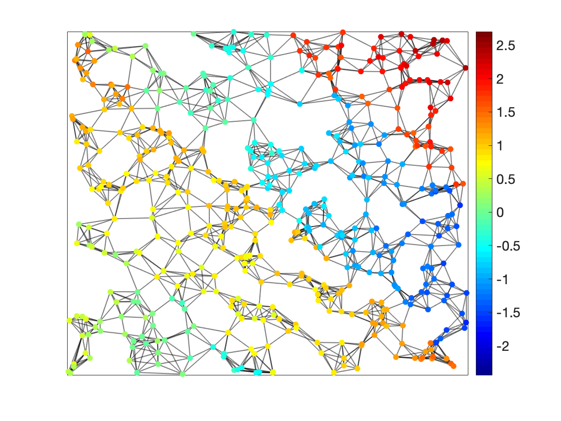
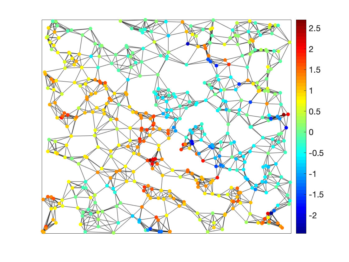
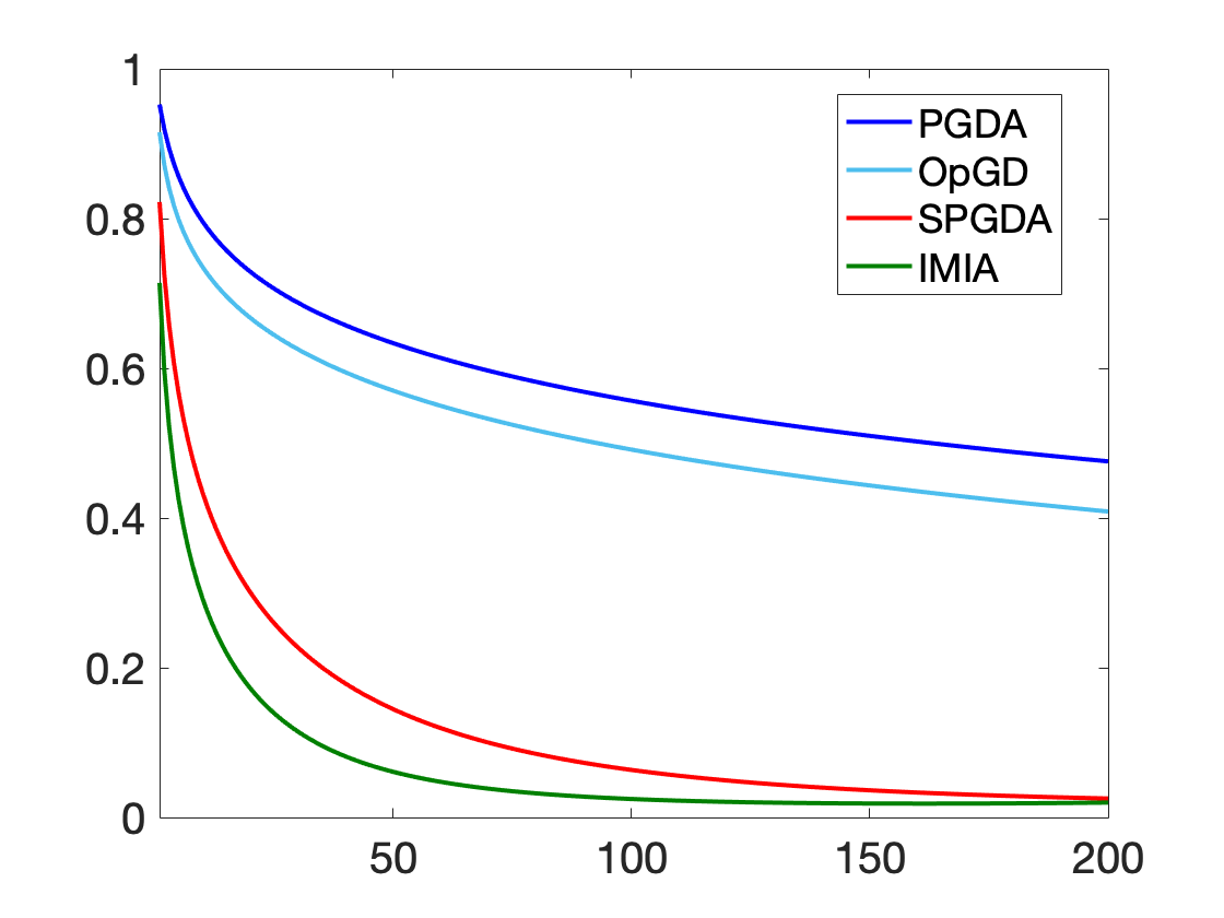
Figure 1: Plotted on the left is a corrupted blockwise polynomial signal ${\bf x}$ and in the middle is the output ${\bf y}={\bf H}{\bf x}$ of the filtering procedure, where $\|{\bf x}\|_{2}=24.8194,\|{\bf y}\|_{2}=21.5317$ and the condition number of the filter ${\bf H}$ is $107.40$. Shown on the right is average of the relative inverse filtering error $E_{2}(m)={\|{\bf x}^{(m)}-{\bf x}\|_{2}}/{\|{\bf x}\|_{2}},1\leq m\leq 200$ over 1000 trials, where $\eta=0.2,\gamma=0.05$ and ${\bf x}^{(m)}$, $m\geq 1$, are the outputs of SPGDA, PGDA, OpGD and IMIA.

Let ${\mathcal{G}}_{512}=(V_{512},E_{512})$ be a random geometric graph with 512 vertices deployed on $[0,1]^{2}$ and an undirected edge between two vertices if their physical distance is not larger than $\sqrt{2/512}$ [11, 22]. In the first simulation, we consider the inverse filtering procedure associated with the graph filter

$${\bf H}={\bf H}_{o}+({\bf L}_{{\mathcal{G}}_{512}}^{\rm sym})^{2},\vspace{-.4em}$$

where ${\bf L}_{{\mathcal{G}}_{512}}^{\rm sym}$ is the normalized Laplacian on the graph ${\mathcal{G}}_{512}$, the filter ${\bf H}_{o}=(H_{o}(i,j))_{i,j\in V_{512}}$ is defined by

$$\hskip-5.78172ptH_{o}(i,j)=\exp\Big{(}-2\times 512\times\|(i_{x},i_{y})-(j_{x},j_{y})\|_{2}^{2}-$$

$$\quad\quad-\frac{\|(i_{x},i_{y})+(j_{x},j_{y})\|_{2}^{2}}{2}\Big{)}+\frac{\gamma_{ij}+\gamma_{ji}}{2},\ \rho(i,j)\leq 2,\vspace{-.3em}$$

$(i_{x},i_{y})$ is the coordinator of a vertex $i\in V_{512}$ and $\gamma_{ij}$ are i.i.d random noises uniformly distributed on $[-\gamma,\gamma]$. Let ${\bf x}_{o}$ be the blockwise polynomial consisting of four strips and imposes $(0.5-2i_{x})$ on the first and third diagonal strips and $(0.5+i_{x}^{2}+i_{y}^{2})$ on the second and fourth strips respectively [11, 19]. In the simulation, the signals

$${\bf x}={\bf x}_{o}+\boldsymbol{\eta}\vspace{-.4em}$$

are obtained by a blockwise polynomial ${\bf x}_{o}$ corrupted by noises $\boldsymbol{\eta}$ with their components being i.i.d. random variables with uniform distribution on $[-\eta,\eta]$, and the observations ${\bf y}$ of the filtering procedure are given by ${\bf y}={\bf H}{\bf x}$, see the left and middle images of Figure 1. In the simulation, we use the SPGDA (III.3) and the PGDA (II.8) with zero initial to implement the inverse filtering procedure ${\bf y}\mapsto{\bf H}^{-1}{\bf y}$, and also we compare their performances with the gradient decent algorithm

$${\bf x}^{(m)}=({\bf I}-\beta_{op}{\bf H}^{T}{\bf H}){\bf x}^{(m-1)}+\beta_{op}{\bf H}^{T}{\bf y},\ m\geq 1\vspace{-.3em}$$ (IV.1)

with zero initial and optimal step length $\beta_{op}$ selected in [12, 19, 20], OpGD in abbreviation, and the iterative matrix inverse approximation algorithm,

$${\bf x}^{(m)}=({\bf I}-\tilde{\bf D}{\bf H}){\bf x}^{(m-1)}+\tilde{\bf D}{\bf y},\ m\geq 1\vspace{-.3em}$$ (IV.2)

IMIA in abbreviation, where ${\bf x}^{(0)}={\bf 0}$ and the diagonal matrix $\tilde{\bf D}$ has entries $H(i,i)/(\sum_{\rho(j,i)\leq 2}|H(i,j)|^{2}),i\in V$, see [10, Eq. (3.4)] with $\tilde{\sigma}=0$. Shown in Figure 1 is the average of the relative inverse filtering error $E_{2}(m),1\leq m\leq 200$ over 1000 trials, and it reaches the relative error 5% at about $57$th iteration for IMIA, 118th iteration for SPGDA, and more than 3000 iterations for PGDA and OpGD. This confirms that ${\bf x}^{(m)},m\geq 1$, in the SPGDA, PGDA, OpGD and IMIA converge exponentially to the output ${\bf x}$ of the inverse filtering, and the convergence rate are spectral radii of matrices ${\bf I}-({\bf P}_{{\bf H}}^{\rm sym})^{-1}{\bf H}$, ${\bf I}-{\bf P}_{{\bf H}}^{-2}{\bf H}^{T}{\bf H}$, ${\bf I}-\beta_{op}{\bf H}^{T}{\bf H}$ and ${\bf I}-\tilde{\bf D}{\bf H}$, see Theorems II.3 and III.1. Here the average of spectral radii in SPGDA, PGDA, OpGD and IMIA are $0.9786,0.9996,0.9993,0.9566$ respectively. We remark that the reason for PGDA and OpGD to have slow convergence in the above simulation could be that their spectral radii are too close to $1$. For the filter perturbation level $\gamma=0.1$, our simulations indicate that for some filters ${\bf H}$ being invertible but not positive definite, the corresponding PGDA and OpGD converge while SPGDA and IMIA diverge.

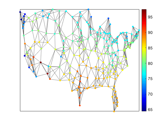
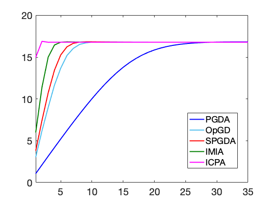
Figure 2: Plotted on the left is the original temperature data ${\bf x}_{12}$. Shown on the right is average of the signal-to-noise ratio $\text{SNR}(m)=-20\log_{10}{\|{\bf x}^{(m)}-{\bf x}_{12}\|_{2}}/{\|{\bf x}_{12}\|_{2}},1\leq m\leq 35$, over 1000 trials, where ${\bf x}^{(m)}$, $m\geq 1$, are the outputs of PGDA, SPGDA, OpGD, IMIA and ICPA, and average of the limit SNR is 16.7869.

Let ${\mathcal{G}}_{T}=(V_{T},E_{T})$ be the undirected graph with 218 locations in the United States as vertices and edges constructed by the 5 nearest neighboring locations, and let ${\bf x}_{12}$ be the recorded temperature vector of those 218 locations on August 1st, 2010 at 12:00 PM, see Figure 2 [19, 23]. In the second simulation, we consider to implement the inverse filtering procedure

$$\tilde{\bf x}=({\bf I}+\alpha{\bf L}_{\mathcal{G}_{T}}^{\rm sym})^{-1}{\bf b}\vspace{-.3em}$$

arisen from the minimization problem

$$\tilde{\bf x}:=\arg\min_{{\bf z}}\|{\bf z}-{\bf b}\|_{2}^{2}+\alpha{\bf z}^{T}{\bf L}_{\mathcal{G}_{T}}^{\rm sym}{\bf z}\vspace{-.3em}$$

in denoising the hourly temperature data ${\bf x}_{12}$, where ${\bf L}_{\mathcal{G}_{T}}^{\rm sym}$ is the normalized Laplacian on ${\mathcal{G}}_{T}$, $\alpha$ is a penalty constraint and ${\bf b}={\bf x}_{12}+\boldsymbol{\eta}$ is the temperature vector corrupted by i.i.d. random noise $\boldsymbol{\eta}$ with its components being randomly selected in $[-\eta,\eta]$ in a uniform distribution [19, 23]. Shown in Figure 2 is the performance of the SPGDA, PGDA, OpGD, IMIA and ICPA to implement the above inverse filtering procedure with noise level $\eta=35$ and the penalty constraint $\alpha=0.9075$ [19], where ICPA is the iterative Chebyshev polynomial approximation algorithm of order one [16, 17, 19]. This indicates that the 3rd term in ICPA, the 5th term in IMIA, the 8th term of SPGDA, the 10th term of OpGD and the 30th term of PGDA can be used as the denoised temperature vector $\tilde{\bf x}$.

To implement the inverse filter procedure (I.5) on SDNs, we observe from the above two simulations that OpGD outperforms PGDA while the selection of optimal step length in OpGD is computationally expensive. If the filter is positive definite, SPGDA, IMIA and ICPA may have better performance than OpGD and PGDA have. On the other hand, SPGDA always converges, but the requirement in [10, Theorem 3.2] to guarantee the convergence of IMIA may not be satisfied and ICPA is applicable for polynomial filters.

References

• [1] J. Yick, B. Mukherjee, and D. Ghosal, “Wireless sensor network survey,” Comput. Netw., vol. 52, no. 12, pp. 2292-2330, Aug. 2008.
• [2] D. I. Shuman, S. K. Narang, P. Frossard, A. Ortega, and P. Vandergheynst, “The emerging field of signal processing on graphs: extending high-dimensional data analysis to networks and other irregular domains,” IEEE Signal Process. Mag., vol. 30, no. 3, pp. 83-98, May 2013.
• [3] R. Hebner, “The power grid in 2030,” IEEE Spectrum, vol. 54, no. 4, pp. 50-55, Apr. 2017.
• [4] C. Cheng, Y. Jiang, and Q. Sun, “Spatially distributed sampling and reconstruction,” Appl. Comput. Harmon. Anal., vol. 47, no. 1, pp. 109-148, July 2019.
• [5] A. Sandryhaila and J. M. F. Moura, “Discrete signal processing on graphs,” IEEE Trans. Signal Process., vol. 61, no. 7, pp. 1644-1656, Apr. 2013.
• [6] A. Sandryhaila and J. M. F. Moura, “Big data analysis with signal processing on graphs: representation and processing of massive data sets with irregular structure,” IEEE Signal Process. Mag., vol. 31, no. 5, pp. 80-90, Sept. 2014.
• [7] A. Ortega, P. Frossard, J. Kovačević, J. M. F. Moura, and P. Vandergheynst, “Graph signal processing: overview, challenges, and applications,” Proc. IEEE , vol. 106, no. 5, pp. 808-828, May 2018.
• [8] M. Coutino, E. Isufi, and G. Leus, “Advances in distributed graph filtering,” IEEE Trans. Signal Process., vol. 67, no. 9, pp. 2320-2333, May 2019.
• [9] J. Jiang, D. B. Tay, Q. Sun and S. Ouyang, “Recovery of time-varying graph signals via distributed algorithms on regularized problems”, IEEE Trans. Signal Inf. Process. Netw., to appear, 2020.
• [10] J. Jiang, and D. B. Tay, “Decentralised signal processing on graphs via matrix inverse approximation,” Signal Process., vol. 165, pp.292-302, Dec. 2019.
• [11] J. Jiang, C. Cheng, and Q. Sun, “Nonsubsampled graph filter banks: theory and distributed algorithms,” IEEE Trans. Signal Process., vol. 67, no. 15, pp. 3938-3953, Aug. 2019.
• [12] S. Chen, A. Sandryhaila, J. M. F. Moura, and J. Kovačević, “Signal recovery on graphs: variation minimization,” IEEE Trans. Signal Process., vol. 63, no. 17, pp. 4609-4624, Sept. 2015.
• [13] E. Isufi, A. Loukas, A. Simonetto, and G. Leus, “Autoregressive moving average graph filtering,” IEEE Trans. Signal Process., vol. 65, no. 2, pp. 274-288, Jan. 2017.
• [14] E. Isufi, A. Loukas, N. Perraudin, and G. Leus, “Forecasting time series with VARMA recursions on graphs,” IEEE Trans. Signal Process., vol. 67, no. 18, pp. 4870-4885, Sept. 2019.
• [15] W. Waheed and D. B. H. Tay, “Graph polynomial filter for signal denoising,” IET Signal Process., vol. 12, no. 3, pp. 301-309, Apr. 2018.
• [16] D. I. Shuman, P. Vandergheynst, D. Kressner, and P. Frossard, “Distributed signal processing via Chebyshev polynomial approximation,” IEEE Trans. Signal Inf. Process. Netw., vol. 4, no. 4, pp. 736-751, Dec. 2018.
• [17] C. Cheng, J. Jiang, N. Emirov, and Q. Sun, “Iterative Chebyshev polynomial algorithm for signal denoising on graphs”, in Proceeding 13th Int. Conf. on SampTA, Bordeaux, France, July 2019, pp. 1-5.
• [18] J. Jiang, D. B. Tay, Q. Sun, and S. Ouyang, “Design of nonsubsampled graph filter banks via lifting schemes,” IEEE Signal Process. Lett., vol. 27, pp. 441-445, Feb. 2020.
• [19] N. Emirov, C. Cheng, J. Jiang, and Q. Sun, “Polynomial graph filter of multiple shifts and distributed implementation of inverse filtering,” arXiv: 2003.11152, Mar. 2020.
• [20] X. Shi, H. Feng, M. Zhai, T. Yang, and B. Hu, “Infinite impulse response graph filters in wireless sensor networks,” IEEE Signal Process. Lett., vol. 22, pp. 1113-1117, Aug. 2015.
• [21] B. Nadler, S. Lafon, I. Kevrekidis, and R. Coifman, “Diffusion maps, spectral clustering and eigenfunctions of Fokker-Planck operators,” In Advances in Neural Information Processing Systems 18, Y. Weiss, B. Schölkopf, and J. Platt eds, MIT Press, Cambridge, 2006, pp. 955-962.
• [22] P. Nathanael, J. Paratte, D. Shuman, L. Martin, V. Kalofolias, P. Vandergheynst, and D. K. Hammond, “GSPBOX: A toolbox for signal processing on graphs,” arXiv:1408.5781, Aug. 2014.
• [23] J. Zeng, G. Cheung, and A. Ortega, “Bipartite approximation for graph wavelet signal decomposition,” IEEE Trans. Signal Process., vol. 65, no. 20, pp. 5466-5480, Oct. 2017.