Optical simulation of atomic decay enhancement and suppression

Abstract

We discuss the decay of a two-level system into an engineered reservoir of coupled harmonic oscillators in the single-excitation manifold and propose its optical simulation with an homogeneous chain of coupled waveguides where individual elements couple to an external waveguide. We use two approaches to study the decay of the optical analogue for the probability amplitude of the two-level system being in the excited state. A Born approximation allows us to provide analytic closed-form amplitudes valid for small propagation distances. A Fourier-Laplace approach allows us to estimate an effective decay rate valid for long propagation distances. In general, our two analytic approximations match our numerical simulations using coupled mode theory and show non-Markovian decay into the engineered reservoir. In particular, we focus on two examples that provide enhancement or suppression of the decay decay rate using flat-top or Gaussian coupling distributions.

I Introduction

Engineered periodic photonic structures provide a robust and highly controllable platform to emulate a wide variety of quantum phenomena related to matter-radiation interactions using classical light Longhi (2009a); Rodríguez-Lara et al. (2018). For example, there exist proposals for photonic analogies to Bloch oscillations Peschel et al. (1998); Morandotti et al. (1999); Pertsch et al. (1999); Lenz et al. (1999); Rodríguez-Lara (2011); Villanueva Vergara and Rodríguez-Lara (2015), quantum collapses and revivals Berry et al. (2001); Longhi (2008), atom-strong-field interactions Longhi et al. (2003); Marangoni et al. (2005); Longhi (2005), Anderson localization Schwartz et al. (2008); Lahini et al. (2008); Thompson et al. (2010), and various models of the Jaynes-Cummings type Longhi (2011); Crespi et al. (2012); Rodríguez-Lara (2014) among others. Such proposals use classical light propagating through arrays of waveguides described by coupled mode theory Snyder (1972); McIntyre and Snyder (1973); Huang (1994) and are amenable to experimental realization via laser inscription techniques Davis et al. (1996); Blömer et al. (2006); Szameit and Nolte (2010). These optical structures offer an immediate and accessible platform to study and visualize new characteristics of their quantum counterparts.

The decay of a quantum emitter coupled to a continuum is an interesting scenario concerning the interaction of matter and radiation. The spin-boson model Leggett et al. (1987); Weiss (2009) is a well-known example of this,

$$\hat{H}= \int_{0}^{\infty}d\omega~{}\left\{\omega\hat{a}^{\dagger}(\omega)\hat{a}(\omega)+g(\omega)\left[\hat{\sigma}_{+}\hat{a}(\omega)+\hat{\sigma}_{-}\hat{a}^{\dagger}(\omega)\right]\right\}+\frac{1}{2}\omega_{0}\hat{\sigma}_{z}.$$ (1)

It models a single two-level system, described by Pauli matrices $\hat{\sigma}_{z}$ and $\hat{\sigma}_{\pm}$ and frequency $\omega_{0}$, linearly coupled with strength $g(w)$ to an environment composed of a continuum of harmonic oscillators, described by creation (annihilation) operators $\hat{a}^{\dagger}$ ($\hat{a}$) and frequency $\omega$. This is the open quantum systems workhorse to study the effects of decoherence and non-Markovian dynamics Shiokawa and Hu (2004); Guarnieri et al. (2016). The fact that it is possible to discretize and unfold the spin-boson model into that of a two-level system interacting with one end of a chain of coupled harmonic oscillators Vojta et al. (2005); Chin et al. (2010); Prior et al. (2010); Woods et al. (2014),

$$\hat{H}= \frac{1}{2}\omega_{0}\hat{\sigma}_{z}+g\left(\hat{\sigma}_{+}\hat{a}_{0}+\hat{\sigma}_{-}\hat{a}^{\dagger}_{0}\right)+\sum_{j=0}^{\infty}\left[\omega_{j}\hat{a}^{\dagger}_{j}\hat{a}_{j}+\gamma_{j}\left(\hat{a}_{j}^{\dagger}\hat{a}_{j+1}+\hat{a}_{j+1}\hat{a}_{j}^{\dagger}\right)\right],$$ (2)

opens the door for the optical simulation of decay from an emitter into engineered environments using, for example, photonic lattices. It allows the visualization and study of effects predicted to arise from impurities embedded within the geometric structure of atoms in a crystal Meade et al. (1995); Garanovich et al. (2012); for example, the theoretical and experimental proposals to realize bound states Longhi (2007a); Plotnik et al. (2011), decay control Dreisow et al. (2008); Longhi (2009b), or Zeno dynamics Longhi (2006, 2007b); Biagioni et al. (2008).

Here, we study the decay of an emitter into an engineered reservoir using an optical analogue for a two-level system coupled to the continuum of states given by a chain of identical oscillators Kockum et al. (2018); Longhi (2020). For the sake of simplicity, an external waveguide takes the role of the two-level emitter and we use the Bloch states of a chain of homogeneously coupled, identical waveguides as the optical analogue of the continuum. We control the placement of some of the chain waveguides around the external waveguide to simulate the interaction between emitter and continuum with engineered coupling profiles leading to non-Markovian decay where we observe enhancement or suppression of the decay. In the following, we describe our quantum model and the continuum of states in the chain, Sec. II. Then, we introduce our optical analogy using coupled mode theory and present two approaches to understand its dynamics, Sec. III. One uses Born approximation to calculate short distance propagation of light in the system. The other uses Fourier-Laplace transform and yields an analytic expression for the leading effective decay rate. In Section IV, we compare our analytic predictions with numerical experiments to good agreement and demonstrate enhancement and suppression of the effective decay rate using two coupling distributions: flat-top and Gaussian. In addition, we show that this phenomenon is robust against noise. Finally, we summarize our findings and state our conclusions in Section V.

II Quantum optics model

We focus on the analysis of a two-level system (TLS) interacting with coupled resonator optical waveguides (CROW)

$$\hat{H}= \sum_{j=-\infty}^{\infty}\left[\gamma\left(\hat{a}_{j}^{\dagger}\hat{a}_{j+1}+\hat{a}_{j+1}\hat{a}_{j}^{\dagger}\right)+g_{j}\left(\hat{\sigma}_{+}\hat{a}_{j}+\hat{\sigma}_{-}\hat{a}^{\dagger}_{j}\right)\right]+\delta\hat{\sigma}_{z},$$ (3)

where the resonators have identical frequency, $\omega$, and creation (annihilation) operators $\hat{a}_{j}^{\dagger}$ ($\hat{a}_{j}$). We consider an homogeneous inter-resonator coupling strength $\gamma$ and a variable coupling strength between the $j$-th resonator and the TLS given by $g_{j}$. This effective Hamiltonian rests in a frame defined by the total excitation number $\hat{N}=\sum_{j}\hat{a}_{j}^{\dagger}\hat{a}_{j}+\hat{\sigma}_{z}/2$ rotating at the frequency of the CROW resonators $\omega$, providing an effective detuning $\delta=(\omega_{0}-\omega)/2$.

As we are interested in the optical simulation of this quantum model, we study its dynamics in the single-excitation manifold,

$$|\psi(t)\rangle=\mathcal{E}_{\alpha}(t)|e,0\rangle+\int_{-\pi}^{\pi}d\phi~{}\mathcal{E}_{\phi}(t)|g,\phi\rangle,$$ (4)

where $|e,0\rangle$ has the TLS in the excited state and the CROW in vacuum and $|g,\phi\rangle$ has the TLS in the ground state and the CROW in a single-excitation Bloch state,

$$|\phi\rangle=\frac{1}{\sqrt{2\pi}}\sum_{k=-\infty}^{\infty}e^{i\phi k}|k\rangle,$$ (5)

where $|k\rangle$ has a single excitation in the $k$-th resonator and the rest in vacuum. Thus, we obtain equations of motion,

$$i\partial_{t}\mathcal{E}_{\alpha}(t)= ~{}\delta\mathcal{E}_{\alpha}(t)+\int_{-\pi}^{\pi}d\varphi~{}G^{\ast}(\varphi)\mathcal{E}_{\varphi}(t),$$ (6)

$$i\partial_{t}\mathcal{E}_{\phi}(t)= ~{}\Omega(\phi)\mathcal{E}_{\phi}(t)+G(\phi)\mathcal{E}_{\alpha}(t),$$ (7)

for the probability amplitude of finding the excitation in the TLS, $\mathcal{E}_{\alpha}$, or in the CROW, $\mathcal{E}_{\phi}$. These amplitudes are given in terms of the effective dispersion relation for the Bloch modes and their coupling strength to the TLS,

$$\Omega(\phi)= ~{}2\gamma\cos\phi,$$ (8)

$$G(\phi)= ~{}\frac{1}{\sqrt{2\pi}}\sum_{k=-\infty}^{\infty}g_{k}e^{i\phi k},$$ (9)

in that order. It is straightforward to argue an optical analogy using classical fields in a whispering gallery mode CROW where an extra resonator is placed close to the CROW to act as the classical analogue of the TLS.

III Coupled Mode Theory Model

Here, our interest lies on the optical simulation of the quantum optical system through arrays of evanescently coupled waveguides. The TLS is simulated by a single waveguide where $g_{j}$ denotes its coupling to the $j$-th waveguide in the chain. The CROW is simulated by an infinite array of identical waveguides with homogeneous first-neighbors coupling $\gamma$. The detuning $\delta=\beta_{0}-\beta$ is the difference between the effective propagation constants of the external waveguide and those in the homogeneous chain. A coupled mode theory analysis for these photonic lattices provides equivalent equations of motion,

$$-i\partial_{z}\mathcal{E}_{\alpha}(z)= ~{}\delta\mathcal{E}_{\alpha}(z)+\int_{-\pi}^{\pi}d\varphi~{}G^{\ast}(\varphi)\mathcal{E}_{\varphi}(z),$$ (10)

$$-i\partial_{z}\mathcal{E}_{\phi}(z)= ~{}\Omega(\phi)\mathcal{E}_{\phi}(z)+G(\phi)\mathcal{E}_{\alpha}(z),$$ (11)

for the modal field amplitudes in the external waveguide and the Bloch modes in the homogeneous chain, $\mathcal{E}_{\alpha}$ and $\mathcal{E}_{\phi}$. These modal field amplitudes play the analogue role of probability amplitudes in the quantum model. We favor photonic lattices as laser writing techniques allow for control of refractive index and placement position of individual waveguides in three dimensions Szameit and Nolte (2010); Gross and Withford (2015). It may be possible to complicate an experimental realization to address, for example, engineered dispersion relations by treating inhomogeneous chains or complex coupling patterns that depend on the propagation direction.

Here, we are interested in simulating the decay of an atomic excitation into an engineered reservoir. In order to provide an analytic guide, we follow an approach similar to that in the study of atomic decay into an oscillator reservoir. First, we take the equation for the optical analogue of the field probability amplitude and integrate it,

$$\!\!\mathcal{E}_{\phi}(z)=e^{i\Omega(\phi)z}\mathcal{E}_{\phi}(0)+iG(\phi)\!\!\int_{0}^{z}\!\!\!d\zeta\,e^{i\Omega(\phi)(z-\zeta)}\mathcal{E}_{\alpha}(\zeta).$$ (12)

Then, we substitute it into the equation for the optical analogue of the TLS excited state probability amplitude,

$$\partial_{z}\mathcal{E}_{\alpha}(z)= \,i\delta\mathcal{E}_{\alpha}(z)+i\int_{-\pi}^{\pi}d\varphi~{}G^{\ast}(\varphi)e^{i\Omega(\varphi)z}\mathcal{E}_{\varphi}(0)-\int_{-\pi}^{\pi}d\varphi~{}\int_{0}^{z}d\zeta~{}|G(\varphi)|^{2}e^{i\Omega(\varphi)(z-\zeta)}\mathcal{E}_{\alpha}(\zeta).$$ (13)

For the sake of simplicity, we focus on an initial condition set where the excitation starts at the waveguide playing the role of the TLS,

$$\mathcal{E}_{\alpha}(0)=1\qquad\mathrm{and}\qquad\mathcal{E}_{\phi}(0)=0.$$ (14)

Under these conditions and upon substitution of all the involved parameters, we obtain an integro-differential equation,

$$\partial_{z}\mathcal{E}_{\alpha}(z)= -\!\!\!\!\sum_{j,k=-\infty}^{\infty}\!\!i^{|k-j|}g_{j}^{\ast}g_{k}\!\int_{0}^{z}\!\!d\zeta\,J_{|k-j|}\left[2\gamma(z-\zeta)\right]\mathcal{E}_{\alpha}(\zeta)+i\delta\mathcal{E}_{\alpha}(z),$$ (15)

in terms of a sum of Bessel functions of the first kind weighted by a product of the coupling strength between individual waveguides in the chain and the external waveguide.

The standard method to solve integro-differential equations of this type is, first, to solve for the analogue of the TLS state probability amplitude,

$$\mathcal{E}_{\alpha}(z)=e^{i\delta z}\left\{1-\sum_{j,k=-\infty}^{\infty}i^{|k-j|}g_{j}^{\ast}g_{k}\int_{0}^{z}d\zeta_{1}~{}\int_{0}^{\zeta_{1}}d\zeta_{2}~{}e^{-i\delta\zeta_{1}}J_{|k-j|}\left[2\gamma(\zeta_{1}-\zeta_{2})\right]\mathcal{E}_{a}(\zeta_{2})\right\}.$$ (16)

Then, iterate the integral term until the solution converges. Here, we restrict ourselves to the scenario where the detuning in the individual propagation constants is larger than the coupling strength between waveguides in the chain and the external waveguide $\delta>g_{j}$. This is an analogy to Born weak-coupling approximation in the quantum system. It yields an approximate solution,

$$\mathcal{E}_{\alpha}^{(1)}(z)\approx e^{i\delta z}\left\{1-\sum_{j,k=-\infty}^{\infty}i^{|k-j|}g_{j}^{\ast}g_{k}\int_{0}^{z}d\zeta_{1}~{}\int_{0}^{\zeta_{1}}d\zeta_{2}~{}e^{i\delta(\zeta_{2}-\zeta_{1})}J_{|k-j|}\left[2\gamma(\zeta_{1}-\zeta_{2})\right]\right\},$$ (17)

where it is not possible to perform Markov approximation in the integral term as it is usually done in the standard atomic decay scenario. Nevertheless, it is possible to solve the integral in the right hand side of this equation if we expand the exponential in its Maclaurin series. This result is valid for small propagation values and it is hard to extract some physical insight from its closed form. Thus, we do not write it here. Instead, we discuss another approach to the solution that provides us with an approximation to the effective decay rate.

Let us start from the differential set in Eq.(10)-(11) and perform a Fourier-Laplace transform Hörmander (1990),

$$\tilde{f}(\zeta) =\int_{0}^{\infty}e^{-i\zeta z}f(z)dz,$$ (18)

that allows us to write the solution for the analogue of the TLS state probability amplitude under the atom decay conditions in Eq. (14),

$$\tilde{\mathcal{E}}_{\alpha}(\zeta) =\frac{-i}{\zeta-\delta-\Sigma(\zeta)},$$ (19)

where we use the shorthand notation for the coupling function

$$\Sigma(\zeta) =\int_{-\pi}^{\pi}\frac{\left|G(\phi)\right|^{2}}{\zeta-\Omega(\phi)}d\phi$$

$$=-i\sum_{j,k=-\infty}^{\infty}\frac{g_{j}g_{k}^{\ast}}{\sqrt{4\gamma^{2}-\zeta^{2}}}e^{-i|j-k|\arccos\frac{\zeta}{2\gamma}}.$$ (20)

It is possible to calculate the inverse Fourier-Laplace transform,

$$f(z)=\frac{1}{2\pi}\int_{-\infty+i\epsilon}^{\infty+i\epsilon}e^{i\zeta z}\tilde{f}(\zeta)d\zeta,$$ (21)

using the formula Visuri et al. (2018),

$$\mathcal{E}_{\alpha}(z)= -\frac{1}{\pi}\int_{-2\gamma}^{2\gamma}e^{i\zeta z}\Im\left[\frac{1}{\zeta-\delta-\Sigma(\zeta)}\right]d\zeta+i2\sum_{k}\mathrm{Res}(\mathcal{\zeta}_{\alpha};z_{k}),$$ (22)

where the first term is an integral around the branch cut defined by the square root in the auxiliary function $\Sigma(\zeta)$ and the second is the sum of residues for the $\alpha$-th pole on the real line outside the branch cut. As the detuning $\delta$ is real, the imaginary part of the coupling $\Sigma(\zeta)$ will rule the decay of the analogue of the TLS excited state probability amplitude and we can approximate,

$$\mathcal{E}_{\alpha}(z)=e^{-\Gamma z}\mathcal{A}(z),\quad\mathrm{with}\quad\Gamma=\Im\left[\Sigma(\delta)\right].$$ (23)

These results, the Born approximation for small propagation distances and the Fourier-Laplace method to approximate the effective decay, allow us to discuss particular examples where the decay can be enhanced or suppressed.

IV Enhancement and Suppression of Decay

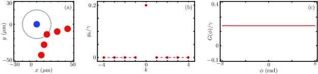
Figure 1: (a) Photonic lattice configuration, (b) coupling strength distribution between individual chain elements and the external waveguide in units of the chain coupling constant $g_{k}/\gamma$, and (c) effective coupling strength between the external waveguide to the Bloch modes of the homogeneous chain in units of the chain coupling constant $G(\phi)/\gamma$.

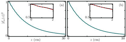
Figure 2: Optical analogue for the probability of finding the TLS in the excited state $|\mathcal{E}_{\alpha}(z)|^{2}$ (a) on-resonance $\delta=0$ and (b) off-resonance with $\delta=0.5\gamma$. We show coupled mode theory results (black solid line), numerical solution to the coupled integro-differential set (completely overlapped with black solid line), analytic solution using the Born approximation $\mathcal{E}_{\alpha}^{(3)}$ (red dashed line), analytic solution using the Fourier-Laplace approach (cyan dotted line) providing field amplitude decay rates (a) $\Gamma=2\times 10^{-2}~{}\gamma$, (b) $\Gamma=2.0656\times 10^{-2}~{}\gamma$.

In order to provide practical examples, we consider a host of single-mode waveguides with circular profile in the weak-guiding regime. For the homogeneous chain, we use cores with refractive index $n_{\mathrm{co}}^{(\mathrm{ch})}=1.4479$ and radius $r_{\mathrm{co}}^{(\mathrm{ch})}=4.5~{}\mu\mathrm{m}$ embedded in cladding with refractive index $n_{\mathrm{cl}}=1.4440$. Each core supports a single $\mathrm{LP}_{01}$ mode at wavelength $\lambda=1550~{}\mathrm{nm}$, the telecommunications C-band. For the waveguides in the homogeneous chain, we set the core to core separation at $d_{\mathrm{ch}}=15~{}\mu\mathrm{m}$. This yields a chain effective propagation constant and coupling strength $\beta=5.85975\times 10^{6}~{}\mathrm{rad}/\mathrm{m}$ and $\gamma=256.635~{}\mathrm{rad}/\mathrm{m}$, in that order. Our numerical coupled mode theory simulations use an homogeneous chain of $501$ elements where the last $20$ waveguides at each end are lossy in order to suppress back-reflections due to finite size.

We focus on two types of coupling strength distributions, flat-top and Gaussian, between individual waveguides of the homogeneous chain and the external waveguide. These are simple to realize in laser written photonic lattices. For each coupling distribution, we study on- and off-resonant scenarios. In the former, the external waveguide is identical to those in the chain. In the latter, the external waveguide has refractive index $n_{\mathrm{co}}^{(\mathrm{e})}=1.44794$ and radius $r_{\mathrm{co}}^{(\mathrm{e})}=4.5~{}\mu\mathrm{m}$ that yield an effective propagation constant $\beta_{0}=5.85988\times 10^{6}~{}\mathrm{rad}/\mathrm{m}$ and a detuning $\delta=0.5\gamma$.

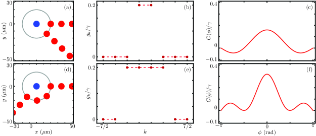
Figure 3: Same as Fig. 1 for (a)-(c) two- and (d)-(f) four-element flat-top coupling distributions.

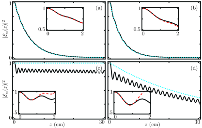
Figure 4: Optical analogue for the probability of finding the TLS in the excited state $|\mathcal{E}_{\alpha}(z)|^{2}$ for the two (a)-(b) and four element (c)-(d) flat-top coupling configurations with (a) and (c) on-resonance, $\delta=0$, and (b) and (d) off-resonance with $\delta=0.5\gamma$. We show coupled mode theory results (black solid line), numerical solution to the coupled integro-differential set (completely overlapped with black solid line), analytic solution using the Born approximation $\mathcal{E}_{\alpha}^{(3)}$ (red dashed line), analytic solution using the Fourier-Laplace approach (cyan dotted line) providing field amplitude decay rates (a) $\Gamma=4\times 10^{-2}~{}\gamma$, (b) $\Gamma=5.1640\times 10^{-2}~{}\gamma$, (c) $\Gamma=0$ and (d) $\Gamma=1.2910\times 10^{-2}~{}\gamma$.

First, we consider a flat-top distribution for the coupling strengths,

$$g_{k}=g\sum_{p=q_{\mathrm{min}}}^{q_{\mathrm{max}}}\delta_{k,p},$$ (24)

where the homogeneous chain elements from position $q_{\mathrm{min}}$ to $q_{\mathrm{max}}$ form a circle of constant radius $r=20.044~{}\mu\mathrm{m}$ around the external waveguide, Fig. 1(a), Fig. 3(a) and Fig. 3(d). This yields a constant coupling strength $g=0.2\gamma$. The scenario where just one waveguide from the homogeneous chain couples to the external waveguide belongs here, Fig. 1(a) and Fig. 1(b). This provides an optical simulation of a TLS coupled to an engineered reservoir such that the coupling strength is constant for all continuous modes, Fig. 1(c). The constant coupling strength $G(\phi)$ allows the use of Markov approximation in the resonant case to calculate the decay rate $\Gamma=g^{2}/(2\gamma)=2\times 10^{-2}~{}\gamma$, Fig. 2(a), which is in accordance with that obtained in the Fourier-Laplace approach,

$$\Gamma(\delta)=\frac{g^{2}}{\sqrt{4\gamma^{2}-\delta^{2}}}.$$ (25)

In this scenario, the off-resonant detuning in the propagation constants induces a slight increase in the effective field amplitude decay rate $\Gamma=2.0656\times 10^{-2}~{}\gamma$, Fig. 2(b).

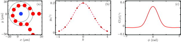
Figure 5: Same as Fig. 1 for Gaussian coupling distribution.

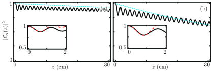
Figure 6: Same as Fig. 3 for couplings given in Fig. 4. The field amplitude decay rates calculated with the Fourier-Laplace approach are (a) $\Gamma=4.7591\times 10^{-4}~{}\gamma$ and (b) $\Gamma=3.0660\times 10^{-3}~{}\gamma$.

Coupling more elements from the homogeneous chain to the external waveguide, Fig. 3(a)-(b) and Fig. 3(d)-(e), simulates a reservoir whose effective coupling does not fulfill the requirements of Markov approximation, Fig. 3(c) and Fig. 3(f). The decay is no longer Markovian, still, it is possible to use Born approximation to good agreement in both on- and off-resonance scenarios, insets in Fig. 4. For two coupled elements, we find an enhancement of the decay rate, compared to the single-waveguide coupling scenario, with the addition of a high frequency oscillation, $\Gamma=4\times 10^{-2}~{}\gamma$ in Fig. 4(a) and $\Gamma=5.1640\times 10^{-2}~{}\gamma$ in Fig. 4(b). For four coupled elements, we find suppression of the decay rates, $\Gamma=0$ in Fig. 4(c) and $\Gamma=1.2910\times 10^{-2}~{}\gamma$ in Fig. 4(d).

Second, we implement a Gaussian distribution for the coupling strengths between elements of the homogeneous chain and the external waveguide,

$$g_{k}=ge^{-\left(\frac{k-p_{0}}{\sigma}\right)^{2}},$$ (26)

where the distribution is centered at the $p_{0}$-th waveguide in the chain and its standard deviation is $\sigma$. For the sake of simplicity, we use the zeroth waveguide as the center of the distribution. The homogeneous chain elements that couple to the external waveguide are distributed between the auxiliary circle defined above and a second auxiliary circle of radius $r=29.7087~{}\mu\mathrm{m}$, Fig. 5(a). This provides us with couplings following a Gaussian distribution, Fig. 5(b), with standard deviation $\sigma=2.31105$ that simulates a reservoir whose effective coupling follows Fig. 5(c). Again, the decay is non-Markovian, Fig. 6, and the decay rate is suppressed compared to the single-waveguide coupling case, $\Gamma=4.7591\times 10^{-4}~{}\gamma$ in Fig. 6(a) and $\Gamma=3.0660\times 10^{-3}~{}\gamma$ in Fig. 6(b).

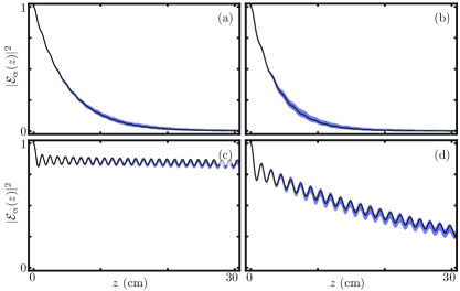
Figure 7: Same as Fig. 4, the black solid line shows the ideal evolution while the light blue region delimits one standard deviation above and below the average of 75 cases with up to $9\%$ random fluctuations in the coupling strength.

Disorder in photonic structures leads to effects like Anderson localization of light De Raedt et al. (1989); Schwartz et al. (2007); Segev et al. (2013) or crosstalk suppression Jaramillo Ávila et al. (2019). Such disorder may arise from manufacturing circumstances; for example, the step precision in the motor controlling laser writing stages Alberucci et al. (2020). For the sake of completeness, we study the effect of random fluctuations in our proposal. In particular, we add $z$-dependent random fluctuations to all the couplings in the chain using a spatial frequency of $81.6895~{}\mathrm{m}^{-1}$ and a maximum fluctuation amplitude of $9\%$, related to deviations of up to $250~{}\mathrm{nm}$ from the ideal position of the waveguides Alberucci et al. (2020). Figure 7 shows the ideal evolution from Fig. 4 and compares it with the region delimited by one standard deviation above and below the average for the evolution of 75 independent cases with such random fluctuations. Decay enhancement or suppression remains even for individual realizations including this type of fabrication imprecision.

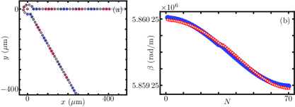
Figure 8: (a) FEM simulation of a normal mode and (b) comparison between effective mode propagation constants from CMT (filled blue dots) and FEM (empty red triangles) for the Gaussian profile in Fig. 5(a), with a total of 70 waveguides.

In addition to the comparison between our analytic approximations and numerical results, we compared between the normal modes calculated using coupled mode theory and a finite element model (FEM) simulation of a smaller system, with only $70$ waveguides, see Fig. 8. We found good agreement between these two approaches further informing ourselves on the validity of our parameter values.

V Conclusion

We study the decay of a two-level system into an engineered continuum reservoir produced by an infinite chain of oscillators. In order to propose an optical analogy using a photonic lattice, we restrict ourselves to the single-excitation manifold. The field amplitude in an external waveguide plays the role of the probability amplitude to find the two-level system in the excited state. The field in a chain of homogeneously coupled waveguides plays the role of the two-level system excitation decaying into an engineered continuum with nonlinear dispersion relation. In addition, we control the placement of the waveguides in the homogeneous chain with respect to the external one to produce different coupling profiles that simulate different coupling profiles between the two-level system and the engineered continuum. Our optical simulation may be experimentally realized by arrays of coupled laser inscribed waveguides.

We explore different coupling profiles. In particular, we discuss flat-top and Gaussian distributions and find non-Markovian decay that leads to enhancement or suppression of the decay rate compared to standard Markovian decay. We implement two analytic approaches that allow us to calculate short-distance propagation and long-distance effective decay rate. We validate these approximations with coupled mode theory numerical simulations for parameters from telecomm C-band experiments.

Exploring the interaction of a quantum system with its environment is a demanding task as these systems are hard to realize in a controlled manner. Optical analogues that simulate reservoir and coupling engineering may aid in this exploration, as they are easier to implement and control in the laboratory, and can provide a platform to benchmark models for system-environment dynamics.

References

References

- Longhi (2009a) S. Longhi, “Quantum-optical analogies using photonic structures,” Laser Photonics Rev. 3, 243 (2009a).
- Rodríguez-Lara et al. (2018) B. M. Rodríguez-Lara, R. El-Ganainy, and J. Guerrero, “Symmetry in optics and photonics: a group theory approach,” Sci. Bull. 63, 244 (2018), arXiv:1803.00121 [physics.optics] .
- Peschel et al. (1998) U. Peschel, T. Pertsch, and F. Lederer, “Optical Bloch oscillations in waveguide arrays,” Opt. Lett. 23, 1701 (1998).
- Morandotti et al. (1999) R. Morandotti, U. Peschel, J. S. Aitchison, H. S. Eisenberg, and Y. Silberberg, “Experimental observation of linear and nonlinear optical Bloch oscillations,” Phys. Rev. Lett. 83, 4756 (1999).
- Pertsch et al. (1999) T. Pertsch, P. Dannberg, W. Elflein, A. Bräuer, and F. Lederer, “Optical Bloch oscillations in temperature tuned waveguide arrays,” Phys. Rev. Lett. 83, 4752 (1999).
- Lenz et al. (1999) G. Lenz, I. Talanina, and C. M. de Sterke, “Bloch oscillations in an array of curved optical waveguides,” Phys. Rev. Lett. 83, 963 (1999).
- Rodríguez-Lara (2011) B. M. Rodríguez-Lara, “Exact dynamics of finite Glauber-Fock photonic lattices,” Phys. Rev. A 84, 053845 (2011), arXiv:1108.3004 [quant-ph] .
- Villanueva Vergara and Rodríguez-Lara (2015) L. Villanueva Vergara and B. M. Rodríguez-Lara, “Gilmore-Perelomov symmetry based approach to photonic lattices,” Opt. Express 23, 22836 (2015), arXiv:1506.02062 [physics.optics] .
- Berry et al. (2001) M. Berry, I. Marzoli, and W. Schleich, “Quantum carpets, carpets of light,” Phys. World 14, 39 (2001).
- Longhi (2008) S. Longhi, “Quantum bouncing ball on a lattice: An optical realization,” Phys. Rev. A 77, 035802 (2008).
- Longhi et al. (2003) S. Longhi, D. Janner, M. Marano, and P. Laporta, “Quantum-mechanical analogy of beam propagation in waveguides with a bent axis: Dynamic-mode stabilization and radiation-loss suppression,” Phys. Rev. E 67, 036601 (2003).
- Marangoni et al. (2005) M. Marangoni, D. Janner, R. Ramponi, P. Laporta, S. Longhi, E. Cianci, and V. Foglietti, “Beam dynamics and wave packet splitting in a periodically curved optical waveguide: Multimode effects,” Phys. Rev. E 72, 026609 (2005).
- Longhi (2005) S. Longhi, “Wave packet dynamics in a helical optical waveguide,” Phys. Rev. A 71, 055402 (2005).
- Schwartz et al. (2008) T. Schwartz, S. Fishman, and M. Segev, “Localisation of light in disordered lattices,” Electron. Lett. 44, 165 (2008).
- Lahini et al. (2008) Y. Lahini, A. Avidan, F. Pozzi, M. Sorel, R. Morandotti, D. N. Christodoulides, and Y. Silberberg, “Anderson localization and nonlinearity in one-dimensional disordered photonic lattices,” Phys. Rev. Lett. 100, 013906 (2008), arXiv:0704.3788 [cond-mat.other] .
- Thompson et al. (2010) C. Thompson, G. Vemuri, and G. S. Agarwal, “Anderson localization with second quantized fields in a coupled array of waveguides,” Phys. Rev. A 82, 053805 (2010).
- Longhi (2011) S. Longhi, “Jaynes-Cummings photonic superlattices,” Opt. Lett. 36, 3407 (2011), arXiv:1111.3457 [physics.atom-ph] .
- Crespi et al. (2012) A. Crespi, S. Longhi, and R. Osellame, “Photonic realization of the quantum Rabi model,” Phys. Rev. Lett. 108, 163601 (2012), arXiv:1111.6424 [quant-ph] .
- Rodríguez-Lara (2014) B. M. Rodríguez-Lara, “Intensity-dependent quantum Rabi model: spectrum, supersymmetric partner, and optical simulation,” J. Opt. Soc. Am. B 31, 1719 (2014), arXiv:1401.7376 [quant-ph] .
- Snyder (1972) A. W. Snyder, “Coupled-mode theory for optical fibers,” J. Opt. Soc. Am. 62, 1267 (1972).
- McIntyre and Snyder (1973) P. D. McIntyre and A. W. Snyder, “Power transfer between optical fibers,” J. Opt. Soc. Am. 63, 1518 (1973).
- Huang (1994) W.-P. Huang, “Coupled-mode theory for optical waveguides: an overview,” J. Opt. Soc. Am. A 11, 963 (1994).
- Davis et al. (1996) K. M. Davis, K. Miura, N. Sugimoto, and K. Hirao, “Writing waveguides in glass with a femtosecond laser,” Opt. Lett. 21, 1729 (1996).
- Blömer et al. (2006) D. Blömer, A. Szameit, F. Dreisow, T. Schreiber, S. Nolte, and A. Tünnermann, “Nonlinear refractive index of fs-laser-written waveguides in fused silica,” Opt. Express 14, 2151 (2006).
- Szameit and Nolte (2010) A. Szameit and S. Nolte, “Discrete optics in femtosecond-laser-written photonic structures,” J. Phys. B: At. Mol. Opt. Phys. 43, 163001 (2010).
- Leggett et al. (1987) A. J. Leggett, S. Chakravarty, A. T. Dorsey, M. P. A. Fisher, A. Garg, and W. Zwerger, “Dynamics of the dissipative two-state system,” Rev. Mod. Phys. 59, 1 (1987).
- Weiss (2009) U. Weiss, Quantum dissipative systems, 4th ed. (World Scientific, Singapore, 2009).
- Shiokawa and Hu (2004) K. Shiokawa and B. L. Hu, “Qubit decoherence and non-Markovian dynamics at low temperatures via an effective spin-boson model,” Phys. Rev. A 70, 062106 (2004), arXiv:quant-ph/0405147 .
- Guarnieri et al. (2016) G. Guarnieri, C. Uchiyama, and B. Vacchini, “Energy backflow and non-Markovian dynamics,” Phys. Rev. A 93, 012118 (2016), arXiv:1510.02333 [quant-ph] .
- Vojta et al. (2005) M. Vojta, N.-H. Tong, and R. Bulla, “Quantum phase transitions in the sub-ohmic spin-boson model: Failure of the quantum-classical mapping,” Phys. Rev. Lett. 94, 070604 (2005), arXiv:cond-mat/0410132 .
- Chin et al. (2010) A. W. Chin, A. Rivas, S. F. Huelga, and M. B. Plenio, “Exact mapping between system-reservoir quantum models and semi-infinite discrete chains using orthogonal polynomials,” J. Math. Phys. 51, 092109 (2010), arXiv:1006.4507 [quant-ph] .
- Prior et al. (2010) J. Prior, A. W. Chin, S. F. Huelga, and M. B. Plenio, “Efficient simulation of strong system-environment interactions,” Phys. Rev. Lett. 105, 050404 (2010), arXiv:1003.5503 [quant-ph] .
- Woods et al. (2014) M. P. Woods, R. Groux, A. W. Chin, S. F. Huelga, and M. B. Plenio, “Mappings of open quantum systems onto chain representations and Markovian embeddings,” J. Math. Phys. 55, 032101 (2014), arXiv:1111.5262 [quant-ph] .
- Meade et al. (1995) R. D. Meade, J. N. Winn, and J. D. Joannopoulos, Photonic crystals: Molding the flow of light, 2nd ed. (Princeton University Press, U.S.A., 1995).
- Garanovich et al. (2012) I. L. Garanovich, S. Longhi, A. A. Sukhorukov, and Y. S. Kivshar, “Light propagation and localization in modulated photonic lattices and waveguides,” Phys. Rep. 518, 1 (2012), arXiv:1107.2992 [physics.optics] .
- Longhi (2007a) S. Longhi, “Bound states in the continuum in a single-level Fano-Anderson model,” Eur. Phys. J. 57, 45 (2007a).
- Plotnik et al. (2011) Y. Plotnik, O. Peleg, F. Dreisow, M. Heinrich, S. Nolte, A. Szameit, and M. Segev, “Experimental observation of optical bound states in the continuum,” Phys. Rev. Lett. 107, 183901 (2011).
- Dreisow et al. (2008) F. Dreisow, A. Szameit, M. Heinrich, T. Pertsch, S. Nolte, A. Tünnermann, and S. Longhi, “Decay control via discrete-to-continuum coupling modulation in an optical waveguide system,” Phys. Rev. Lett. 101, 143602 (2008).
- Longhi (2009b) S. Longhi, “Optical analogue of coherent population trapping via a continuum in optical waveguide arrays,” J. Mod. Optic. 56, 729 (2009b).
- Longhi (2006) S. Longhi, “Nonexponential decay via tunneling in tight-binding lattices and the optical Zeno effect,” Phys. Rev. Lett. 97, 110402 (2006).
- Longhi (2007b) S. Longhi, “Control of photon tunneling in optical waveguides,” Opt. Lett. 32, 557 (2007b).
- Biagioni et al. (2008) P. Biagioni, G. Della Valle, M. Ornigotti, M. Finazzi, L. Duo, P. Laporta, and S. Longhi, “Experimental demonstration of the optical Zeno effect by scanning tunneling optical microscopy,” Opt. Express 16, 3762 (2008).
- Kockum et al. (2018) A. F. Kockum, G. Johansson, and F. Nori, “Decoherence-free interaction between giant atoms in waveguide quantum electrodynamics,” Phys. Rev. Lett. 120, 140404 (2018), arXiv:1711.08863 [quant-ph] .
- Longhi (2020) S. Longhi, “Photonic simulation of giant atom decay,” Opt. Lett. 45, 3017 (2020).
- Gross and Withford (2015) S. Gross and M. J. Withford, “Ultrafast-laser-inscribed 3D integrated photonics: challenges and emerging applications,” Nanophotonics 4, 332 (2015).
- Hörmander (1990) L. Hörmander, The Analysis of Linear Partial Differential Operators. I, Distribution Theory and Fourier Analysis, 2nd ed., Grundlehren Der Mathematischen Wissenschaften (Springer, Germany, 1990).
- Visuri et al. (2018) A.-M. Visuri, C. Berthod, and T. Giamarchi, “Impurity coupled to a lattice with disorder,” Phys. Rev. A 98, 053607 (2018), arXiv:1807.07744 [cond-mat.quant-gas] .
- De Raedt et al. (1989) H. De Raedt, A. Lagendijk, and P. de Vries, “Transverse localization of light,” Phys. Rev. Lett. 62, 47 (1989).
- Schwartz et al. (2007) T. Schwartz, G. Bartal, S. Fishman, and M. Segev, “Transport and Anderson localization in disordered two-dimensional photonic lattices,” Nature 446, 52 (2007).
- Segev et al. (2013) M. Segev, Y. Silberberg, and D. N. Christodoulides, “Anderson localization of light,” Nat. Photonics 7, 197 (2013).
- Jaramillo Ávila et al. (2019) B. Jaramillo Ávila, J. M. Torres, R. de J. León-Montiel, and B. M. Rodríguez-Lara, “Optimal crosstalk suppression in multicore fibers,” Sci. Rep. 9, 15737 (2019), arXiv:1905.09416 [physics.optics] .
- Alberucci et al. (2020) A. Alberucci, N. Alasgarzade, M. Chambonneau, M. Blotheand H. Kämmer, G. Matthäus, C. P. Jisha, and S. Nolte, “In-depth optical characterization of femtosecond-written waveguides in silicon,” Phys. Rev. Appl. 14, 024078 (2020).