Flexible nonstationary spatio-temporal modeling of high-frequency monitoring data

Abstract

Many physical datasets are generated by collections of instruments that make measurements at regular time intervals. For such regular monitoring data, we extend the framework of half-spectral covariance functions to the case of nonstationarity in space and time and demonstrate that this method provides a natural and tractable way to incorporate complex behaviors into a covariance model. Further, we use this method with fully time-domain computations to obtain bona fide maximum likelihood estimators—as opposed to using Whittle-type likelihood approximations, for example—that can still be computed efficiently. We apply this method to very high-frequency Doppler LIDAR vertical wind velocity measurements, demonstrating that the model can expressively capture the extreme nonstationarity of dynamics above and below the atmospheric boundary layer and, more importantly, the interaction of the process dynamics across it.

Keywords: Spectral domain, Doppler LIDAR, Meteorology, Atmospheric Boundary Layer

1 Introduction

Gaussian process (GP) models are versatile and useful tools for studying spatial and spatio-temporal processes. A GP model is completely specified by postulating a mean and covariance function, so that a collection of data points $\bm{y}=\left\{y_{j}\right\}_{j=1}^{N}$ observed at locations $\left\{\bm{x}_{j}\right\}_{j=1}^{N}$ has the distribution

$$\bm{y}\sim\mathcal{N}(\bm{\mu},\bm{\Sigma}),$$

where $\bm{\mu}(\bm{x})$ is a mean function and $\bm{\Sigma}_{j,k}=K(\bm{x}_{j},\bm{x}_{k})$ is the covariance matrix induced by covariance function $K$. A common estimation problem is to select a parametric form for $K$ and attempt to recover the parameters from data. For the duration of this paper, we assume $\bm{\mu}\equiv 0$. While this may seem restrictive, the analysis of anomaly fields instead of raw data is commonplace, and extensions of these methods to a nonzero mean would not be overly difficult.

If $K(\bm{x},\bm{y})$ is a function only of $\bm{x}-\bm{y}$, we call the process model stationary, an assumption which is enormously useful for a variety of both theoretical and computational reasons. For the vast majority of real-world processes, however, even among the ones for which a Gaussian process assumption is tolerable, a stationarity assumption is not. With modern computing tools and instrument infrastructure, spatial datasets are commonly large enough and dense enough that even visual inspection of the data will make it abundantly clear that a stationary process model would be fundamentally misrepresentative of the dynamics of the process. For this reason, developing natural and flexible nonstationary models to more accurately capture dependence structure in modern datasets is an exigent statistical problem.

Modeling such nonstationarity is difficult, however, in no small part because it is challenging to specify valid covariance models via positive definite functions. In the stationary case, perhaps the easiest way to verify that a function $K_{\bm{\theta}}$ is a valid covariance function is to find an integrable function for which $K$ in its one-argument form $K_{\bm{\theta}}(\bm{x},\bm{y})\equiv K_{\bm{\theta}}(\bm{x}-\bm{y})$ is its Fourier transform. One can then express $K_{\bm{\theta}}$ as

$$K_{\bm{\theta}}(\bm{s})=\int e^{i2\pi\left\langle\bm{f},\bm{s}\right\rangle}S_{\bm{\theta}}(\bm{f})\mathrm{d}\bm{f},$$

where $S_{\bm{\theta}}(\bm{f})$ is called the spectral density corresponding to $K$. If $S_{\bm{\theta}}(\bm{f})$ is positive and symmetric about zero, Bochner’s theorem implies that $K_{\bm{\theta}}$ is a positive definite real-valued function and thus a valid covariance function. In general, it is easier to specify positive and symmetric functions than positive definite ones, and many of the more exotic stationary covariance functions are derived, or at least confirmed to be valid, in the spectral domain. Many theoretical results about GPs that are relevant to the parameter estimation problem, like those about the equivalence and orthogonality of Gaussian measures, are proven and applied in the spectral domain (Ibragimov & Rozanov 1978, Stein 1999, Zhang 2004, Zhang & Zimmerman 2005), further emphasizing that the spectral domain is arguably often a more productive way to approach studying covariance structure.

Unfortunately, nonstationarity implies the nonexistence of a spectral density, and the full-dimensional Fourier transform of most covariance functions only exists in the distributional sense. Accordingly, it is necessary to find other ways to specify valid models, and there is a wealth of literature in the field that contributes methods and ideas towards solving this problem. Examples include careful stitching together of valid “local” models (Higdon 2002, Stein 2005a, Paciorek & Schervish 2006), deforming the coordinate system of a stationary process (Genton & Perrin 2004, Anderes & Stein 2008), spatial mixtures of different stationary fields (Fuentes & Smith 2001), nonparametric representations (Sampson & Guttorp 1992, Jun & Stein 2008), multiresolution models (Nychka et al. 2002, Matsuo et al. 2011, Katzfuss 2017), Bayesian methods (Katzfuss & Cressie 2012), separable models (Genton 2007), and many others. But each method has drawbacks, and for some it is difficult to compute true maximum likelihood estimators, so that approximated likelihoods are commonly substituted. With this in mind, we extend a methodology for continuing to think about nonstationary covariances in the spectral domain by modeling marginal spectra and coherences. Like every other method listed here, this strategy has its limitations and is not always available or prudent to use. It does, however, provide a way to incorporate and potentially compose several different ways of specifying nonstationarity and, as will be shown here, can be pushed into complex forms while maintaining validity, numerical robustness, and expressiveness.

2 Half-spectral covariance functions

A key observation made in Cressie & Huang (1999) and Stein (2005b) is that one can obtain a valid model by specifying a “half-spectral” form of a covariance function for a random field $Z(t,\bm{x})$, whereupon the stationary space-time covariance function is obtained by performing an inverse Fourier transform of a function $h(f,\bm{x}-\bm{x}^{\prime})$ with respect to time. The function

$$K(t-t^{\prime},\bm{x}-\bm{x}^{\prime}):=\int_{\Omega}e^{2\pi if(t-t^{\prime})}h(f,\bm{x}-\bm{x}^{\prime})\mathrm{d}f$$ (2.1)

gives a valid covariance function for discrete-time data ($\Omega=[-1/2\Delta t,1/2\Delta t)$) or continuous-time data ($\Omega=\mathbb{R}$). In discrete time, we advocate using $\sin(\pi f)$ instead of $f$ so that the periodic extension of the model is smooth with respect to $f$ at the endpoints. Stein (2005b) proposes an expression for $h$ of the form

$$h(f,\bm{x}-\bm{x}^{\prime})=S(f)C_{f}(\bm{x}-\bm{x}^{\prime})e^{ig(f)\bm{u}^{T}(\bm{x}-\bm{x}^{\prime})}$$

for a stationary but non-separable and asymmetric model, where $S(f)$ can be interpreted to be a marginal spectral density in time; $C_{f}$—a valid spatial correlation function—is the modulus of the coherence of $Z(\cdot,\bm{x})$ and $Z(\cdot,\bm{x}^{\prime})$; and $g(f)\bm{u}^{T}(\bm{x}-\bm{x}^{\prime})$ is the phase relation. Varying $C_{f}$ in (2.1) allows flexibility in the nature of nonseparability, with separability being the special case of $C_{f}$ and $g(f)$ not depending on $f$.

For measurements made at regular time intervals and a relatively small number of spatial locations, this modeling perspective can be considered as an augmented multiple time series approach for which incorporating new time series (measurements at a new spatial location) is possible in a model-consistent way and without the requirement of any new parameters. It affords the practitioner a convenient and approachable method for modeling space-time dependence primarily by thinking about marginal—or at least lower-dimensional—dependence structure. If the data is regular in time, for example, one can visually inspect marginal time spectra and immediately include features of those estimates in a valid, fully spatio-temporal covariance model. See Horrell & Stein (2017) for an extension to more complex stationary models of this form and Guinness & Stein (2013) for a nonstationary model in a similar vein.

We now extend this modeling framework to the case of processes that are nonstationary in space but stationary in time. Because this modeling perspective relies so heavily on specifying marginals, a nonstationary extension is very direct.

Theorem 1.

Let $\left\{S_{\bm{x}}(f)\right\}$ be temporal spectral densities indexed by spatial locations $\bm{x}$. If $C_{f}(\bm{x},\bm{x}^{\prime})$ is a real-valued correlation function and $g(f)$ is an odd function, then

$$K((t,\bm{x}),(t^{\prime},\bm{x}^{\prime}))=\int_{\Omega}e^{i2\pi f(t-t^{\prime})+ig(f)\bm{u}^{T}(\bm{x}-\bm{x}^{\prime})}\sqrt{S_{\bm{x}}(f)S_{\bm{x}^{\prime}}(f)}C_{f}(\bm{x},\bm{x}^{\prime})\mathrm{d}f$$ (2.2)

defines a valid covariance function for a spatially nonstationary real-valued space-time process $Z(t,\bm{x})$.

Proof.

As in the proof provided in Stein (2005b), we consider the matrix-valued function

$$\bm{\Phi}(f):=\left\{\sqrt{S_{\bm{x}_{j}}(f)S_{\bm{x}_{k}}(f)}C_{f}(\bm{x}_{j},\bm{x}_{k})e^{ig(f)\bm{u}^{T}(\bm{x}_{j}-\bm{x}_{k}^{\prime})}\right\}_{j,k=1}^{n}.$$ (2.3)

It is sufficient to prove that $\bm{\Phi}(f)$ is positive semi-definite for each $f$ and integrable. Note that we may write $\bm{\Phi}(f)=\bm{\mathcal{S}}(f)\circ\bm{C}(f)\circ\mathcal{P}(f)$, a Hadamard product of the time-spectra term, correlation function, and phase term. $\bm{C}(f)$ is by definition positive definite, and we note that $\bm{\mathcal{S}}(f)$ is positive semi-definite by recognizing the rank one structure of $\bm{\mathcal{S}}(f)=\bm{u}(f)\bm{u}(f)^{T}$ with $\bm{u}_{j}(f)=\sqrt{S_{\bm{x}_{j}}(f)}$. Similarly, $\mathcal{P}(f)$ has a Hermitian rank-one symmetric factorization since $e^{ig(f)\bm{u}^{T}(\bm{x}-\bm{x}^{\prime})}=e^{ig(f)\bm{u}^{T}\bm{x}}e^{-ig(f)\bm{u}^{T}\bm{x}^{\prime}}$. By the Schur product theorem, then, we conclude that $\bm{\Phi}(f)$ is positive semi-definite for all $f$. Since $\sqrt{S_{\bm{x}_{j}}(f)S_{\bm{x}_{k}}(f)}\leq\max_{j}S_{\bm{x}_{j}}(f)$ is integrable and both $C_{f}$ and the complex exponential are bounded, $\bm{\Phi}(f)$ is integrable. Finally, we observe that $\bm{\Phi}(f)=\overline{\bm{\Phi}(-f)}$ and thus conclude that K is a real-valued positive definite function. ∎

Several comments are in order. First, the proof of Theorem 1 demonstrates that this argument extends to a much broader class of functions than the one that will be studied here. For example, an algebraic representation of $\bm{\mathcal{S}}(f)=\bm{Q}(f)\bm{A}(f)\bm{Q}(f)^{T}$ where $\bm{A}$ is positive semidefinite could provide an even richer nonparametric representation for marginal and cross spectra of a spatio-temporal process. Building rank-deficient positive semi-definite matrices is easy, and per the argument of the proof above, such an extension would also yield an equally valid real-valued covariance function.

Second, temporal stationarity—or at most a restrictive form of nonstationarity—is required by this model. Most importantly, the existence of a spectral density is an implication of stationarity along that dimension. It is of course possible to have processes that are locally stationary but whose spectra evolve slowly and continuously with time (as were studied in Poppick et al. (2016), for example), but even this extension would substantially complicate the numerics required to build covariance matrices for maximum likelihood. Further, as will be discussed below, performing space-time domain computations with this model with minimal numerical concerns is only made feasible by the use of the Fast Fourier Transform algorithm (Cooley & Tukey 1965). This means that the covariance function can only conveniently be evaluated at the inverse Fourier frequencies, and so other relaxations of temporal stationarity like deformation-type methods would also be difficult to apply.

Finally, we note that the above argument still applies if $C_{f}$ is a bounded covariance function and not a correlation function, and that requiring it to be a correlation function primarily serves to mitigate identifiability problems. Moreover, $C_{f}$ need not be stationary. As will be demonstrated later in this work, between the space-dependent marginal time spectra $S_{\bm{x}}$ and a nonstationary coherence function $C_{f}(\bm{x},\bm{x}^{\prime})$, it is easily possible to compose this model with other nonstationary models to obtain an even more flexible valid covariance function.

Despite the difficulty discussed above, there are several restrictive ways to relax the temporal stationary of this model. While slightly more complex and involved ideas are possible, in this work we only employ the simplest possible extension in the form of a nonstationary scale.

Corollary 1.

If $K$ is the function given in (2.2) and $\lambda(\bm{x},t)\geq 0$ everywhere, then the function

$$\tilde{K}((\bm{x},t),(\bm{x}^{\prime},t^{\prime})):=\lambda(\bm{x},t)\lambda(\bm{x}^{\prime},t^{\prime})K((\bm{x},t),(\bm{x}^{\prime},t^{\prime}))+\eta^{2}\bm{1}_{\left\{(\bm{x},t)=(\bm{x}^{\prime},t^{\prime})\right\}}$$ (2.4)

is also a valid covariance function.

With the further addition of a “temporal nugget” $\eta_{t}^{2}\bm{1}_{\left\{t=t^{\prime}\right\}}$, in the same spirit as the “spatial nugget” of Gneiting (2002), this model is precisely the formulation we use here to explore our data.

For a relatively small number of spatial locations, using the FFT to numerically evaluate these integrals for all pairs of spatial locations and then to assemble covariance matrices is straightforward. With little numerical work, then, one can write simple models for marginal—or at least lower-dimensional—behavior and obtain all the function values necessary to build a valid space-time covariance matrix in $\mathcal{O}(n_{s}^{2}n_{t}\log_{2}n_{t})$ time complexity, where $n_{s}$ is the number of unique spatial locations and $n_{t}$ is the time width of the process. In particular, the integral approximation for discrete-time processes given by

$$\int_{-1/2}^{1/2}e^{2\pi ift}g(\sin\pi f)df\approx\frac{1}{N}\sum_{j=0}^{N-1}e^{2\pi if_{j}t}g(\sin\pi f_{j})$$

for Fourier frequencies $\left\{f_{j}\right\}$ can be evaluated simultaneously and efficiently at all necessary time lags $t$ via the inverse FFT algorithm. This is effectively an application of trapezoidal integration, and by also taking sufficiently long FFTs to avoid edge effects, these approximations can easily be made accurate to double precision for kernels that can be checked with a closed form expression. In our experience, taking an FFT length of $N=7\cdot n_{t}$ is more than sufficient. To the degree that any linear algebra for large ill-conditioned matrices is exact in finite precision arithmetic, then, the evaluation of the likelihood with covariance matrices assembled from this approximation is exact. As further evidence of this, the log-likelihood for FFT sizes ranging from $5\cdot n_{t}$ to $21\cdot n_{t}$ all agree to at least single precision in our experimentation, further suggesting that this numerical scheme provides effectively exact function evaluation and thus provides a way to minimize the exact likelihood.

Despite the many FFTs being computed here, in our use case with on the order of $30$ spatial locations and one thousand time locations, evaluating the function at all necessary space-time locations and aggregating the values takes less than one second on a Dell Latitude E5470 with an Intel Core i5-6200U@2.3GHz CPU, a mobile processor not designed for heavy computation, and poses no numerical or computational challenge. Once these values (and the values for the derivatives of (2.4) with respect to kernel parameters) have been computed, covariance matrices can be assembled and the likelihood and its derivatives can be evaluated as usual.

To motivate the application of this model, let us introduce the dataset to be explored in this work.

3 Doppler LIDAR wind measurement data

The US Department of Energy’s Atmospheric Radiation Measurement (ARM) program was created with the goal to provide long-term in situ and remotely sensed observations in various climate regimes to improve the understanding of processes impacting atmospheric radiation (Stokes & Schwartz 1994). The Southern Great Plains (SGP) observatory is the first ARM site and the largest climate research facility in the world, equipped with more than 50 instruments and providing continuous measurements ranging from basic meteorology and radiation to cloud and aerosol properties at several locations in the north-central Oklahoma and south Kansas region (Mather & Voyles 2013, Sisterson et al. 2016). In this work, we study measurements of the vertical component of the wind field at very high spatio-temporal resolution as observed by the $1.5\text{\,}\mathrm{\SIUnitSymbolMicro m}$ pulsed Doppler lidar (DL) deployed at the SGP central facility (CF).

The principle of operation of the DL is similar to that of the Doppler radars in that they both transmit pulses of energy into the atmosphere and measure the returned signal scattered back by clear-air irregularities (Gage & Balsley 1978, Muradyan & Coulter 2020). In other words, scattering is assumed to originate from atmospheric particulates moving at the same speed as the wind. The ARM DL has a full upper-hemispheric scanning capability, measuring the one-dimensional velocity projections across a range of angles in order to fully resolve the three-dimensional wind field (Newsom 2012). The general DL scanning strategy for this purpose at the SGP CF is to perform 8-beam plan-position-indicator scans once every approximately 15 minutes, and all sampling between those times is done in a vertically staring mode. When the DL is pointing vertically, it provides height- and time-resolved measurements of the vertical velocity.

As we focus exclusively on vertical measurements here, the resulting data from this instrument is multiple gappy time series of the vertical wind velocity components at $30\text{\,}\mathrm{m}$ vertical intervals (commonly referred to as “range gates”), which extend to a maximum of $9.6\text{\,}\mathrm{km}$ range and are sampled at approximately $1.2$ second intervals. For more details about the instrument’s theory of operation, functionality, and configuration, see Newsom (2012). Figure 1 shows an example collection of time series plots of the data at discrete range gates over the duration of fifteen minutes on June 2, 2015, while Figure 2 shows the time-height cross-section of the same data from about $200\text{\,}\mathrm{m}$ to $2.25\text{\,}\mathrm{km}$ above ground level (AGL).

Figure 1: Fifteen minutes of Doppler LIDAR vertical wind velocity measurements at several different range gates on June $2$, $2015$ at $1400$UTC, shortly after sunrise.

As one would expect, this data exemplifies extreme nonstationarity, which no sensible model could ignore. In space, the primary source of nonstationarity is the height of the atmospheric boundary layer (ABL), which is the layer directly in contact with the earth’s surface through turbulent mixing processes (Tucker et al. 2009). As can be seen in Figure 2 below, the ABL height increases during the day via solar heating of the surface, resulting in a well-mixed daytime convective boundary layer (BL). In the absence of solar radiation at night, the convection is stopped by heat loss to space, resulting in a thin nocturnal BL with typically $100300\text{\,}\mathrm{m}$ depth (Cushman-Roisin 2014). Above the BL height, the concentrations of particulates such as aerosols and cloud particles, which are the source of scattering, dramatically decrease, resulting in a substantial reduction in the backscatter signal and thus measurement quality. Typically, only the lowest $2$ to $3\text{\,}\mathrm{km}$ of the atmosphere yields high-quality measurements (Newsom 2012). In addition, the minimum range for the DL is approximately $100\text{\,}\mathrm{m}$, and even if data is available below that height, the lowest range gates are suspect and are recommended not to be used (personal communicaton with instrument mentor). As the maximum operational range of the ARM DL is up to $9.6\text{\,}\mathrm{km}$, this is a substantial truncation, but inspection of the data on its full domain would involve a great deal of preprocessing measurement artifacts, which is outside the scope of this work.

In order to study the dependence structure across the BL and capture the dynamics above and below simultaneously without having to contend too deeply with measurement quality concerns or computational issues, we focus this work on the time $1400$ UTC—shortly after the local sunrise in northern Oklahoma—when the ABL height has grown to approximately $400500\text{\,}\mathrm{m}$ on average. This part of the day is convenient as the ABL height is well above the minimum altitude of DL operation, so that plenty of high-quality measurements are available below it as well as above it. For the purpose of manageable data sizes, we focus on altitudes between about $200$ and $850\text{\,}\mathrm{m}$ in order to have large spatial samples of range gates both above and below the BL while also being able to work with full measurement segments between 3D scans. For reference, considering range gates $7$ to $28$ and a full time segment of vertical measurements (about $14$ minutes) amounts to approximately $17$ thousand data points.

Figure 2: An alternative view of the process from $1300$ to $1600$ UTC on June $24$th, $2015$, a day with particularly high activity, demonstrating the rising mixing height after sunrise and the dynamic domain of data reliability. The color scale for this image is highly truncated, as the unreliable measurements at altitudes with low SNR range sporadically between $20\text{\,}\mathrm{m}\text{/}\mathrm{s}$ and $-20\text{\,}\mathrm{m}\text{/}\mathrm{s}$.

This data source has several features and properties that make it interesting to study. For one, the spatial component is vertical and not horizontal. Just as time should not be treated as just another spatial dimension, we believe that the vertical dimension of many physical processes should be treated with the same care. The measurements here provide a good testing set for vertical modeling as well as a strong justification of this claim, as the spatial nonstationarity is very sharp and likely not even once differentiable, which is unusual to observe on such a fine spatial scale and with such high covariance.

As well as being uncommon in its spatial axis, this data source is a good motivating example for nonstationary models. The rate at which marginal dynamics change is noticeably faster than the rate at which covariance information decays, which is to say that two range gates can have obviously different dynamics but still be strongly informative about each other. The measurements at $300$ and $480\text{\,}\mathrm{m}$ in Figure 1, for example, clearly have very strong coherence at low frequencies despite how different finer-scale behavior is at each altitude. Any locally stationary model would necessarily be throwing out a great deal of information of that kind, which is arguably of the highest scientific interest. In some cases, the creation of intricate nonstationary models has been criticized for not actually capturing more behavior, as it is frequently the case that most information that can be learned about a spatial or spatio-temporal process corresponds to high frequency behavior of the spectral density (or is otherwise “micro-ergodic”), which thus largely corresponds to local information (Stein 1999). This data is an example of a situation when that type of pessimism is unnecessary.

Finally, the measurements used in this work are made at a much higher frequency than most other sources of environmental data. At the time scales of these measurements, a great deal can be inferred about smoothness properties of the field, as well as the study of wind gusts, turbulence and other small-scale meteorological phenomena, which will especially be critical in the lower portion of the ABL. In general, the features that require high-frequency resolution to observe also make the data more challenging to study. Things like measurement quantization when the wind velocity is very low at night, for example, are real concerns, as well as distinguishing real short time-scale velocity fluctuations from instrument noise. As will be clear, this work is only scratching the surface of what can be studied with this type of high-frequency and high-resolution monitoring data, and it is precisely its associated challenges that make it interesting.

4 A half-spectral model for Doppler LIDAR data

One of the strongest features of the data, as can be seen in Figure 2, is the strong low-frequency coherence across the entire domain, but especially above the ABL. Another is that the scale of the measurements appears to decay as the altitude increases above the ABL height. For the purposes of both parameter economy and interpretability, we introduce first a functional form that we use extensively in several parts of this model. Taking inspiration from the frequency response function of the Butterworth filter from signal processing (Butterworth 1930), whose signature feature is being flat in some neighborhood of zero and then decaying algebraically, we define the utility function $B(z)$ as

$$B(z;\xi_{0},\xi_{1},\xi_{2}):=e^{\xi_{0}}\left[1+\left(\frac{z}{\xi_{1}}\right)^{2\xi_{2}}\right]^{-1}.$$

As we demonstrate below, this function is convenient in three different parts of the specification of the model given by Equation 2.4.

With that preliminary complete, let us begin by specifying a form for the nonstationary scale parameters, which we choose to represent in a flexible form as

$$\lambda(x,t)=B((x-\beta)_{+}\;;\;0,\phi_{1},\phi_{2})\sum_{j=1}^{4}w_{j}(t)\theta_{t_{j}},$$

where $\left\{t_{j}\right\}$ are knots in time chosen evenly across the domain, and $w_{j}(t)$ are time-dependent weights that are normalized to sum to one, with unnormalized forms given by $\tilde{w}_{j}(t):=e^{-|t-t_{j}|/50\Delta t}$ (for reference, the time window for the data that will ultimately be fitted here is about $775\Delta t$). The spatial dependence of the scale comes in the form of the Butterworth-type function $B$, which starts to decay once the altitude $x$, in units of meters, is above the ABL height, which we denote with $\beta$, and is itself a model parameter. Due to the structure we see across several days of data, we prefer this representation for the spatial dependence on scale to knot-based function approximation.

To introduce spatial nonstationarity of components in the marginal spectrum and coherence while maintaining interpretability, we implement a very simple space-dependent parameter mapping given by, for example with the parameter $\rho$,

$$\rho(x):=(1-w(x))\rho_{0}+w(x)\rho_{1},$$

where

$$w(x):=(1+e^{-\tau(x-\beta)})^{-1},$$ (4.1)

and the subscripts $0$ and $1$ denote in this case the regimes of being below and above the ABL respectively, so that effectively the spatially-indexed parameters are logistic interpolants between two values. The inverse scale parameter $\tau$ of this logistic function is informative about the sharpness of the transition from below-ABL and above-ABL dynamics, and is very important to this model. For one reason, fixing a constant ABL height $\beta$ for $15$ minutes is obviously not correct from a brief inspection of Figure 2. Since that is a form of temporal nonstationarity that this model cannot easily account for, we introduce this $\tau$ parameter to at least allow the model the ability to communicate about the sharpness of this transition and capture better the dynamics at range gates near the mean height of the ABL.

Equipped with this parametric form of spatial dependence, we define the marginal spectral densities with

$$S_{x}(f)=(1+B(\sin\pi f\;;\;\xi_{0}(x),\xi_{1},\xi_{2}))(e^{\rho(x)}\sin^{2}\pi f+1)^{-\nu(x)-1/2},$$ (4.2)

where the spatial dependence of the low frequency multiplier $1+B$ comes in the form of the parameter $\xi_{0}(x)$, and $\xi_{1}$ and $\xi_{2}$ are fixed across space. As a small technical note, for time series measured at non-unit time steps, a change of variables in the Fourier transform suggests that a $\Delta t$ rescaling should be applied to $S_{x}$. We do not do that here and instead elect to simply treat the time sampling as unit sampling and scale nonparametric spectral density estimators consistently with that in the following section, implicitly absorbing this $\Delta t\approx 1.2$s into the $\theta_{j}$ parameters.

This spectral density corresponds closely to a filtered Matérn spectral density for continuously indexed processes, which is best characterized by its algebraic decay, so that $S(\bm{f})\sim\left\|\bm{f}\right\|_{2}^{-2\nu-d}$ in $d$ dimensions. In discrete time, $\nu$ is not so directly interpretable since even negative values yield spectral densities corresponding to non-pathological processes. But the algebraic tail decay is nonetheless convenient and at least heuristically informative about smoothness that would be implied by a continuous version of the model, and using $\sin\pi f$ instead of $f$ extends this functional form nicely to a function that is smooth on the unit torus. The extra multiplier of $1+B$ provides the model the ability to add extra low frequency energy without affecting the higher frequencies, which is a pronounced feature of the data and can be seen in the diagnostic figures of the next section.

The coherence function $C_{f}$ is crucial to this model, and is extremely different above and below the ABL. To be as flexible as possible, we choose $C_{f}$ to be a nonstationary Paciorek-Schervish-type correlation function with an extension to variable smoothness (Stein 2005a) given by

$$C_{f}(x,x^{\prime}):=\frac{\sqrt[4]{\gamma(x)\gamma(x^{\prime})}}{\gamma(x,x^{\prime})}\mathcal{M}_{(\nu_{s}(x)+\nu_{s}(x^{\prime}))/2}\left(\frac{|x-x^{\prime}|}{\gamma(x,x^{\prime})}\right),$$ (4.3)

where $\gamma(x,x^{\prime}):=\sqrt{(\gamma(x)+\gamma(x))/2}$, and we parameterize

$$\gamma(x)(f):=B(\sin\pi f;\;\zeta_{0}(x),\zeta_{1}(x),\zeta_{2}(x)),$$

using $\zeta$ instead of $\xi$ to distinguish between the parameters of $B(f)$ for $S_{x}$ and $C_{f}$. Unfortunately the spatially indexed smoothnesses for $C_{f}$ are not smoothly interpolated like other spatially indexed parameters in order to avoid taking derivatives of second-kind Bessel functions (refer to the Discussion section for more information) in the derivatives of $C_{f}$, and are instead discontinuously parameterized as

$$\nu_{s}(x)=\mathbf{1}\left\{x\leq\beta\right\}\frac{1}{2}+(1-\mathbf{1}\left\{x\leq\beta\right\})\frac{3}{4}.$$

We acknowledge that it is somewhat noteworthy to have fixed smoothnesses for this correlation function. Considering that there are only approximately $20$ spatial locations being considered in this model, however, our experimentation indicates that the effect of varying these parameters on the likelihood is modest.

Since the true phase dynamics of this process are almost certainly driven by nonlinearity that no Gaussian process model could capture, we include only the simplest form of $g(f)$ in this model, setting $g(f):=\alpha\sin\pi f$, with no spatial variation. With the inclusion of our space-time and temporal nuggets, we now have a complete covariance function of the form (2.4). Table $1$ provides a final summary and reference for the interpretation of each parameter in the model.

$\beta$	Boundary layer height
$\tau$	Shape parameter for boundary layer regime transition rate
$\theta_{t_{j}}$	Local scale parameters
$\phi_{j}$	Scale decay with altitude over boundary layer
$\xi_{j}(x)$	Space-dependent shape parameters for temporal low-frequency multipler $1+B(f)$
$\rho(x)$	Space-dependent temporal range-type parameter
$\nu(x)$	Space-dependent temporal smoothness-type parameter
$\zeta_{j}(x)$	Space-dependent shape parameters for coherence function $\gamma(x)$
$\alpha$	Phase function rate-type parameter
$\eta_{st}$	Spatio-temporal nugget size
$\eta_{t}$	Purely temporal nugget size

Table 1: A summary of all the parameters used in the covariance model as parameterized in (2.4).

With this model fully introduced, it merits comment that since it will be fitted with maximum likelihood estimators, parameters informing the high frequency behavior will be highly priotized over parameters that inform low frequency behavior. Because of the human tendency to focus on lower frequency behavior when performing visual inspection of simulations or other diagnostics, however, we have included several parameters and degrees of freedom here that do not heavily affect the likelihood. The $\left\{\xi(x)\right\}$ parameters, for example, are a good example of extra degrees of freedom that do not strongly affect the likelihood and are completely confined to the very lowest of frequencies. Their effect on visual diagnostics for conditional simulations, however, are very noticeable. For certain purposes, a smaller model could be used with similarly satisfying results, and the supplemental information compares visual diagnostics of the full model shown here and a reduced one. Since this work is an investigation into how well a Gaussian process model can capture the very complex dynamics of vertical wind velocity, however, we proceed with a maximalist approach here.

5 Estimation Results

Using the methods described at the end of section $2$, it is possible to evaluate the likelihood and its derivatives entirely in the space-time domain. In this section, we discuss the results of maximum likelihood estimation for the above model to six different days of data in June $2015$ that were judged to have comparable meteorological conditions. In each case, we performed the optimization over the $25$ parameters using a hand-written trust region method adapted directly from Nocedal & Wright (2006). In order to only use first derivatives of the covariance function with respect to parameters, we used a symmetrized stochastic estimator for the expected Fisher information matrix (Geoga et al. 2019) as an approximation for the Hessian (observed information). To further avoid costly matrix-matrix operations, we also used a symmetrized stochastic gradient. Optimization was terminated at a relative precision of $10^{-6}$ in the objective function.

To enable unconstrained optimization, the model was fitted with transformed variables, as many need to be positive. This was necessary due to the stochastic derivative estimators, as several parameters being reasonably close to zero means that even a very accurate stochastic gradient and expected Fisher matrix can cause domain issues. All point estimates and standard deviations provided in this section, however, are provided for the model as parameterized above, obtained by un-transforming the computed MLE and evaluating the likelihood and its derivatives once in that domain. This is not ideal considering that high-quality convergence criteria such as the size of the Newton step change in response to a nonlinear transformation of the variables, but we do not believe this issue to be overly invalidating in the interpretation of the estimates or their associated uncertainty. The code used to perform the estimation is spread out over the software packages HalfSpectral.jl for the half-spectral kernel function and GPMaxlik.jl for efficient optimization of the likelihood, both written in the Julia programming language (Bezanson et al. 2017). Example files in HalfSpectral.jl contain some specific scripts used to obtain the estimates below.

As described in Section $3$, we restrict the estimation here to approximately $14$ minute time segments (about $780$ measurements) and range gates between $210\text{\,}\mathrm{m}$ (the seventh gate) and either $690\text{\,}\mathrm{m}$ (the $23$rd gate) or $840\text{\,}\mathrm{m}$ (the $28$th gate) based on the height of the ABL so that both above- and below-mixing height dynamics have reasonable representation. These time segements correspond to measurements between the gaps noted previously, and the resulting data sizes are near the limit of the computational abilities of the hardware used for the estimation. We do stress, however, that the methods described here could equally well be applied to gappy regular monitoring data by virtue of the fact that performing the computations in the time domain means that an FFT is being applied to the analytical spectrum, not the data itself.

Table 2: Results from maximum likelihood estimation of the six days that were studied. Standard deviations obtained via the stochastic expected Fisher matrix are provided in parentheses.

$1.055\,626\,208\,760\,271\,5$ ($0.026\,424\,298\,766\,574\,53$)$0.722\,996\,251\,355\,872\,6$ ($0.088\,928\,562\,936\,467\,52$)$1.030\,186\,644\,934\,802\,7$ ($0.032\,989\,068\,519\,742\,12$)$1.127\,122\,386\,652\,885\,2$ ($0.023\,099\,720\,549\,153\,64$)$1.650\,984\,240\,180\,638\,3$ ($0.028\,403\,158\,632\,165\,71$)$1.543\,598\,265\,435\,324\,4$ ($0.036\,234\,368\,095\,309\,96$) $\theta_{t_{2}}$$1.181\,608\,341\,826\,014\,8$ ($0.027\,966\,037\,586\,357\,417$)$0.616\,923\,120\,889\,336\,2$ ($0.089\,600\,364\,562\,101\,84$)$1.225\,918\,303\,818\,577\,5$ ($0.034\,777\,977\,360\,913\,565$)$0.917\,768\,497\,616\,781\,1$ ($0.025\,601\,825\,905\,434\,982$)$1.780\,315\,176\,207\,628\,6$ ($0.029\,463\,409\,312\,946\,054$)$1.232\,669\,144\,567\,845\,3$ ($0.038\,188\,657\,787\,520\,37$) $\theta_{t_{3}}$$1.266\,068\,293\,208\,684\,2$ ($0.027\,916\,400\,371\,029\,864$)$0.635\,597\,630\,804\,224\,6$ ($0.089\,550\,349\,423\,295$)$1.626\,750\,203\,523\,075\,2$ ($0.034\,381\,799\,852\,393\,11$)$1.161\,379\,251\,653\,029\,7$ ($0.024\,741\,167\,106\,438\,887$)$1.858\,777\,257\,563\,530\,8$ ($0.029\,517\,967\,936\,912\,044$)$1.252\,365\,950\,166\,914\,4$ ($0.037\,916\,529\,005\,101\,34$) $\theta_{t_{4}}$$1.189\,610\,654\,842\,628\,2$ ($0.026\,263\,241\,978\,222\,388$)$0.824\,548\,347\,204\,948\,6$ ($0.088\,913\,355\,661\,829\,42$)$1.979\,833\,792\,541\,656\,3$ ($0.032\,614\,136\,786\,900\,81$)$1.264\,061\,949\,615\,961\,5$ ($0.022\,959\,968\,385\,943\,76$)$2.264\,140\,123\,708\,678\,7$ ($0.028\,220\,857\,609\,009\,838$)$0.874\,126\,028\,741\,982\,1$ ($0.036\,804\,450\,300\,389\,51$) $\rho_{0}$$2.718\,453\,552\,351\,492\,3$ ($0.140\,643\,595\,265\,621\,17$)$0.352\,379\,143\,629\,287\,5$ ($0.496\,833\,605\,596\,710\,4$)$3.476\,935\,558\,561\,451\,4$ ($0.144\,652\,300\,033\,813\,57$)$2.368\,616\,665\,065\,095$ ($0.114\,208\,094\,805\,316\,73$)$2.757\,604\,293\,733\,935\,6$ ($0.133\,670\,681\,503\,409\,66$)$2.863\,413\,789\,112\,529$ ($0.157\,145\,625\,967\,273\,27$) $\nu_{0}$$1.143\,637\,684\,123\,136\,8$ ($0.058\,287\,478\,028\,003\,215$)$7.071\,036\,700\,136\,331\,5$ ($2.534\,591\,305\,764\,318$)$1.023\,075\,217\,155\,951\,6$ ($0.041\,882\,662\,488\,122\,3$)$1.427\,851\,074\,192\,237$ ($0.065\,645\,081\,784\,998\,27$)$1.210\,833\,944\,826\,796\,6$ ($0.054\,117\,649\,305\,205\,906$)$1.345\,209\,228\,510\,582$ ($0.066\,590\,875\,311\,083\,75$) $\rho_{1}$$5.525\,591\,539\,265\,126$ ($0.175\,382\,654\,961\,793\,4$)$2.310\,759\,437\,801\,987\,6$ ($0.546\,079\,313\,763\,527\,4$)$6.761\,163\,700\,459\,53$ ($0.118\,446\,373\,557\,162\,09$)$8.926\,909\,979\,121\,648$ ($0.151\,262\,679\,573\,608\,42$)$4.885\,356\,713\,012\,435$ ($0.179\,978\,266\,700\,268\,37$)$6.246\,958\,603\,234\,542\,6$ ($0.188\,486\,284\,697\,332\,72$) $\nu_{1}$$2.139\,742\,354\,992\,843$ ($0.175\,395\,546\,690\,502\,03$)$20.052\,700\,039\,213\,416$ ($9.774\,254\,200\,268\,746$)$3.136\,564\,803\,509\,157\,3$ ($0.187\,443\,437\,477\,930\,27$)$0.371\,209\,470\,709\,341$ ($0.025\,830\,281\,901\,005\,607$)$2.113\,313\,519\,968\,596$ ($0.167\,712\,388\,596\,908$)$2.351\,354\,024\,441\,731\,5$ ($0.248\,941\,628\,833\,581\,84$) $\zeta_{00}$$12.456\,481\,904\,932\,77$ ($0.494\,636\,495\,745\,386\,5$)$13.637\,335\,735\,835\,578$ ($0.177\,180\,340\,923\,441\,6$)$0.496\,812\,859\,113\,053$ ($27\,107.970\,539\,093\,55$)$17.465\,524\,606\,902\,807$ ($0.886\,036\,522\,343\,168\,8$)$11.890\,452\,625\,368\,212$ ($0.293\,794\,705\,341\,327\,84$)$11.482\,418\,807\,490\,845$ ($0.442\,480\,215\,602\,140\,35$) $\zeta_{01}$$0.016\,520\,131\,519\,287\,76$ ($0.005\,620\,330\,799\,788\,851$)$0.010\,484\,992\,424\,042\,2$ ($0.002\,098\,428\,389\,374\,461\,8$)$0.033\,184\,699\,415\,237\,71$ ($0.005\,245\,187\,155\,527\,688$)$0.000\,208\,538\,240\,859\,707\,04$ ($0.000\,120\,300\,717\,803\,678\,99$)$0.070\,397\,495\,529\,311\,38$ ($0.012\,665\,293\,648\,571\,704$)$0.020\,008\,578\,723\,901\,934$ ($0.007\,655\,091\,635\,413\,272\,5$) $\zeta_{02}$$0.839\,564\,101\,909\,488\,4$ ($0.046\,384\,969\,836\,582\,48$)$0.771\,455\,075\,261\,889\,2$ ($0.043\,845\,982\,420\,887\,45$)$1.353\,570\,734\,601\,728$ ($0.060\,320\,627\,814\,665\,46$)$0.681\,784\,500\,113\,789\,3$ ($0.034\,942\,528\,971\,098\,764$)$1.088\,385\,197\,329\,873\,3$ ($0.055\,523\,159\,724\,022\,15$)$0.726\,648\,928\,877\,398\,6$ ($0.053\,009\,587\,316\,248\,41$) $\zeta_{10}$$16.793\,176\,920\,400\,71$ ($0.502\,266\,010\,961\,236\,7$)$13.568\,906\,732\,409\,545$ ($0.213\,843\,068\,559\,753\,57$)$18.133\,182\,962\,067\,444$ ($0.329\,197\,794\,536\,130\,24$)$24.814\,625\,240\,050\,45$ ($0.843\,653\,431\,181\,234$)$14.952\,590\,939\,136\,945$ ($0.307\,496\,290\,552\,448\,7$)$17.253\,802\,286\,249\,76$ ($0.491\,237\,254\,602\,323\,8$) $\zeta_{11}$$0.011\,595\,522\,882\,194\,436$ ($0.002\,511\,051\,743\,530\,177\,4$)$10.657\,394\,685\,525\,706$ ($3.524\,882\,488\,558\,071$)$0.000\,531\,487\,546\,840\,966\,5$ ($0.000\,193\,340\,123\,997\,305\,3$)$1.501\,157\,775\,293\,706\,610-5$ ($1.002\,894\,718\,379\,586\,710-5$)$0.039\,116\,551\,317\,130\,5$ ($0.004\,538\,829\,409\,167\,363$)$0.004\,385\,388\,344\,358\,817$ ($0.001\,090\,989\,900\,762\,981$) $\zeta_{12}$$1.383\,669\,202\,874\,107$ ($0.094\,231\,851\,676\,865\,03$)$69.027\,321\,851\,221\,91$ ($23.142\,467\,575\,824\,526$)$0.674\,281\,776\,776\,612\,2$ ($0.056\,924\,421\,911\,040\,85$)$1.022\,605\,305\,539\,614\,3$ ($0.048\,635\,544\,935\,276\,54$)$1.861\,159\,227\,408\,659\,7$ ($0.124\,002\,075\,661\,488\,59$)$0.970\,383\,928\,988\,044$ ($0.098\,188\,734\,845\,412\,8$) $\beta$$458.841\,071\,692\,587$ ($2.147\,502\,500\,896\,736$)$659.988\,129\,793\,974\,6$ ($4.099\,071\,131\,641\,573\,6$)$472.421\,412\,257\,123\,4$ ($3.181\,003\,466\,565\,874$)$682.399\,434\,990\,027$ ($1.232\,985\,853\,847\,615\,3$)$583.808\,869\,171\,055\,3$ ($3.493\,247\,794\,791\,414\,7$)$545.734\,517\,263\,595\,8$ ($3.944\,843\,080\,162\,433\,7$) $\tau$$0.056\,450\,164\,194\,192\,13$ ($0.002\,072\,203\,297\,736\,497\,2$)$0.040\,726\,982\,903\,226\,12$ ($0.002\,356\,610\,706\,978\,164$)$0.023\,901\,573\,736\,095\,35$ ($0.000\,776\,216\,563\,548\,962\,6$)$0.027\,046\,521\,963\,850\,24$ ($0.000\,447\,090\,005\,716\,045\,1$)$0.033\,306\,456\,786\,019\,53$ ($0.001\,315\,975\,743\,894\,569\,7$)$0.036\,040\,049\,780\,895\,01$ ($0.001\,277\,559\,747\,029\,874\,8$) $\xi_{00}$$3.578\,639\,178\,296\,149$ ($0.855\,745\,806\,702\,676\,5$)$18.982\,493\,267\,434\,105$ ($8.801\,716\,889\,295\,792$)$1.022\,912\,561\,381\,477\,3$ ($0.388\,702\,040\,588\,540\,9$)$14.940\,267\,793\,718\,695$ ($5.071\,835\,072\,114\,729$)$0.468\,116\,943\,579\,591\,4$ ($0.223\,110\,361\,518\,101\,43$)$37.069\,669\,719\,082\,33$ ($22.654\,546\,983\,234\,997$) $\xi_{01}$$7.076\,909\,630\,417\,635$ ($1.918\,324\,190\,944\,924$)$9.213\,539\,692\,471\,493$ ($4.724\,728\,718\,719\,655$)$0.020\,060\,935\,968\,813\,08$ ($0.233\,714\,342\,882\,645\,23$)$38.478\,107\,546\,027\,05$ ($14.238\,775\,076\,964\,256$)$1.574\,493\,891\,076\,900\,6$ ($0.609\,719\,257\,012\,627\,4$)$38.305\,892\,677\,745\,945$ ($24.499\,053\,550\,449\,357$) $\xi_{2}$$6.552\,778\,376\,515\,583$ ($2.930\,354\,073\,713\,726\,6$)$0.851\,916\,410\,720\,768\,3$ ($0.131\,141\,035\,298\,827\,1$)$12.982\,330\,294\,317\,986$ ($36.070\,558\,871\,422\,75$)$1.090\,548\,229\,751\,948\,7$ ($0.182\,571\,625\,034\,329\,92$)$5.987\,846\,877\,884\,677$ ($4.896\,466\,751\,271\,616$)$0.825\,318\,386\,968\,373\,9$ ($0.167\,083\,883\,049\,729\,35$) $\xi_{1}$$0.031\,432\,735\,240\,416\,2$ ($0.001\,856\,508\,010\,748\,643\,5$)$0.042\,607\,013\,039\,939\,51$ ($0.008\,387\,984\,848\,445\,816$)$0.020\,258\,817\,911\,405\,59$ ($0.002\,305\,710\,282\,458\,664$)$0.006\,805\,909\,471\,948\,028$ ($0.002\,029\,818\,682\,411\,227\,4$)$0.062\,462\,804\,280\,392\,456$ ($0.005\,614\,437\,628\,270\,14$)$0.002\,236\,474\,979\,156\,914\,4$ ($0.001\,361\,725\,469\,508\,449\,7$) $\phi_{1}$$106.556\,309\,905\,563\,14$ ($17.669\,285\,010\,950\,023$)$163.164\,296\,899\,874\,4$ ($17.630\,958\,187\,670\,95$)$225.680\,958\,469\,609\,98$ ($48.730\,490\,455\,517\,2$)$4.097\,526\,441\,846\,528\,5$ ($0.954\,251\,610\,251\,357\,7$)$107.684\,550\,726\,430\,69$ ($28.438\,806\,242\,750\,694$)$362.178\,581\,387\,904\,7$ ($45.747\,826\,330\,598\,706$) $\phi_{2}$$0.635\,972\,549\,073\,775\,1$ ($0.072\,992\,378\,039\,115\,89$)$1.203\,634\,030\,582\,968\,5$ ($0.272\,726\,806\,008\,042\,1$)$1.033\,383\,962\,894\,429$ ($0.325\,089\,430\,329\,806\,03$)$0.452\,868\,700\,374\,407$ ($0.035\,036\,802\,955\,833\,86$)$0.507\,617\,981\,210\,592\,2$ ($0.058\,467\,987\,657\,412\,23$)$1.137\,723\,704\,502\,574\,5$ ($0.393\,536\,019\,585\,896\,8$) $\alpha$$0.000\,213\,876\,148\,836\,481\,38$ ($0.000\,309\,209\,490\,061\,952\,57$)$0.000\,120\,742\,993\,604\,908\,5$ ($0.000\,134\,730\,742\,432\,832\,37$)$0.001\,827\,496\,398\,862\,378$ ($0.000\,336\,671\,994\,763\,312\,8$)$0.000\,692\,324\,390\,926\,253\,4$ ($0.000\,241\,056\,547\,679\,610\,1$)$0.000\,420\,883\,926\,094\,765\,04$ ($0.000\,194\,922\,731\,763\,093\,06$)$1.089\,373\,877\,613\,205\,210-5$ ($0.000\,265\,868\,560\,146\,854\,6$) $\eta_{st}$$0.035\,915\,930\,482\,619\,51$ ($0.000\,370\,518\,758\,114\,994\,5$)$0.110\,607\,859\,089\,434\,25$ ($0.001\,040\,560\,022\,762\,987\,7$)$0.024\,901\,597\,093\,122\,09$ ($0.000\,222\,718\,841\,763\,561\,18$)$0.066\,759\,462\,711\,712\,74$ ($0.000\,728\,196\,518\,310\,915\,2$)$0.056\,924\,525\,967\,230\,97$ ($0.000\,630\,908\,343\,579\,931\,3$)$0.071\,076\,968\,915\,724\,79$ ($0.000\,552\,664\,113\,101\,976\,2$) $\eta_{t}$$0.013\,877\,115\,982\,555\,983$ ($0.000\,693\,584\,826\,281\,175\,2$)$0.048\,576\,498\,205\,722\,44$ ($0.002\,007\,837\,052\,098\,120\,3$)$0.007\,468\,919\,813\,436\,987$ ($0.000\,433\,890\,860\,020\,708\,17$)$0.031\,288\,611\,541\,286\,22$ ($0.001\,395\,997\,264\,942\,208\,3$)$0.023\,329\,184\,634\,585\,37$ ($0.001\,103\,323\,531\,151\,892$)$0.028\,578\,073\,495\,440\,157$ ($0.001\,137\,862\,911\,016\,672\,8$)

Table 5 summarizes the point estimates for each day and provides the implied standard deviation from the expected Fisher matrix. Using this matrix as a proxy for the precision matrix of the MLE is a nontrivial approximation, considering that the necessary conditions for that to even hold asymptotically—for example, the log-likelihood looking quadratic near the MLE—are likely not met, or at least are not met for this data size. Nonetheless, as the expected Fisher matrix is the inverse of the Godambe information matrix for the score equations, it still serves an at least somewhat informative purpose about the uncertainty of each point estimate (Heyde 2008, Stein et al. 2013).

One main takeaway from these tables is that the parameters seem to be estimated reasonably precisely and have believable values, although of interest is the fact that for most days, there is at least one parameter that is not well-resolved, and it is not always the same parameter. In some sense we find this encouraging, as it is likely an unreasonable expectation that for a priori domain choices every parameter is resolvable across any nontrivial collection of days due to the domain variability discussed earlier. Robustness to this issue seems to be a more important and realistic priority than full resolution at every day and in all conditions. Further, the inconsistencies between which parameters are not well-resolved serve as at least an indirect indication that a model much simpler than the one used here would likely sacrifice some degrees of freedom that maximum likelihood does consider to be valuable in at least some circumstances.

Perhaps the most interesting of these estimates in its day-to-day variability is the time-marginal smoothness-type parameter $\nu$. On June $20$th, $\nu$ is quite low above the ABL, paradoxically indicating a rougher field above the ABL height than below it. This is surprising, as from both a heuristic application of meteorological principles and a visual inspection of the data, one might expect $\nu$ above the ABL to be reasonably large, and certainly larger than $\nu$ below the ABL. Moreover, considering that there are two nugget-type terms, it is noteworthy that maximum likelihood chose to represent the behavior of this field in $\nu$. This contrasts with the estimates for June $03$, where maximum likelihood did precisely the opposite: the estimated $\nu$ parameters are very large, but so are the nugget parameters compared to the other days. The variability of this parameter is particularly of interest considering that its continuous analog informs very important properties of the process, such as differentiability.

Figure 3: The correlation matrix of the MLE of the model for the data on June $02$.

Several other parameters vary interestingly across days. The parameters corresponding to marginal spectra do not vary in shocking ways, although the $\left\{\xi\right\}$ parameters—which only inform additional very low frequency power—appear to be reasonably sensitive to the particular structure of the fifteen minute segments. While phase parameters often do not strongly influence the likelihood, it is worth noting that for one of the six days (June $06$) the MLE suggests a slight but well-estimated phase asymmetry. Finally, we observe that the coherence parameters for the process above the ABL are particularly interesting for June $03$. Specifically, the MLE suggests that the coherence function above the ABL is almost flat at a value quite close to $1$, suggesting a sort of deterministic process whose randomness comes largely from the two nugget parameters. While it is obvious that coherence is high at low frequencies above the ABL, it is noteworthy that for one of the days—and only one of the days—maximum likelihood selected that type of structure.

Figure 4: Marginal spectra for gates above the ABL (blue/squares) and below the ABL (red/circles) on June $02$. Analytical estimates for these spectra (including nugget parameters) are overlaid as lines of corresponding colors. Estimators from individual range gates are shown faintly in grey.

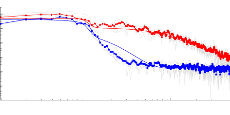
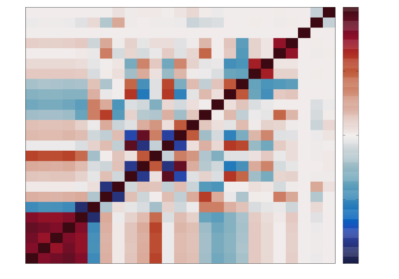
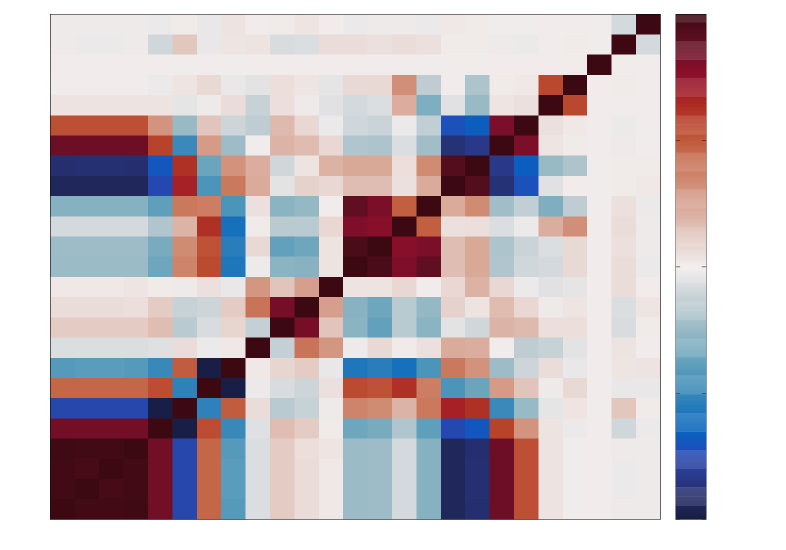
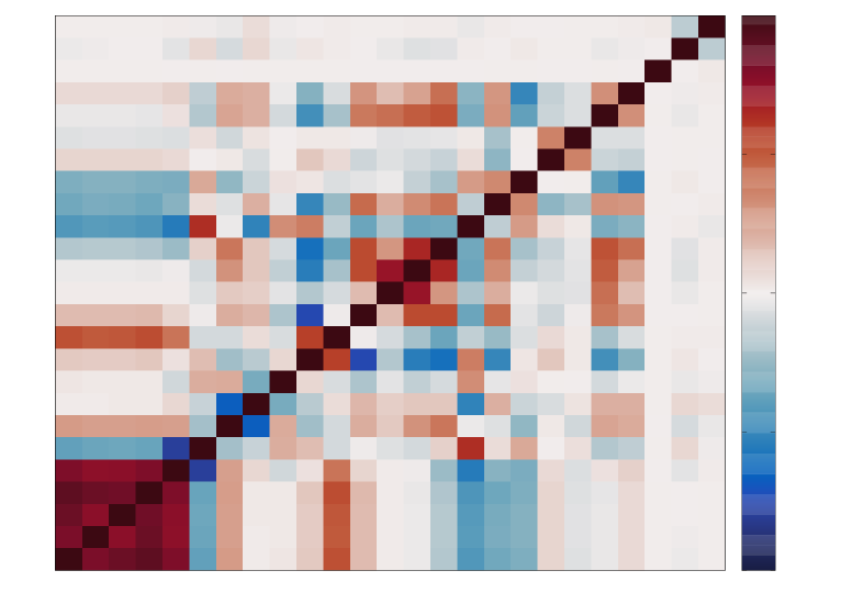
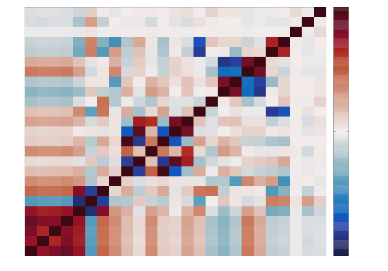
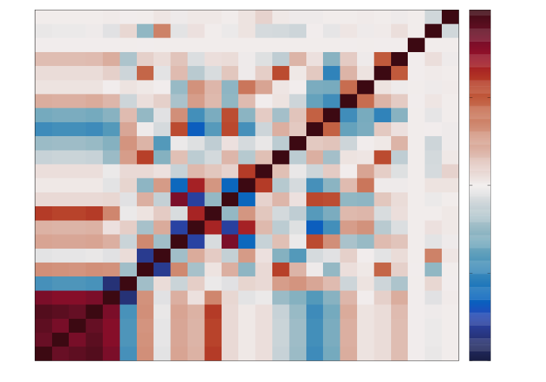
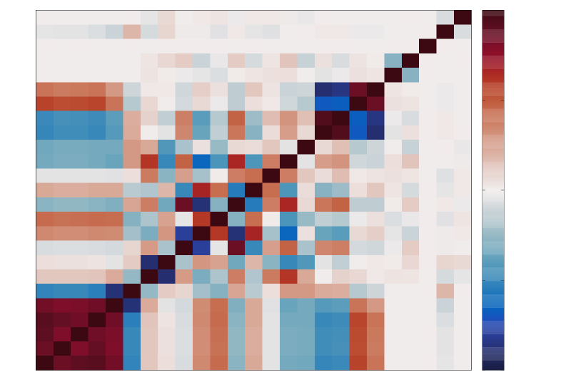
Figure 3 shows the correlation (not covariance) matrix for the MLE on June $02$. As one might expect, the parameters determining the effectively nonparametric scale function are highly correlated and are inversely correlated with the smoothness, as is the range-type parameter $\rho$. These types of correlation structure are quite common in stationary Matérn-type models. Moreover, there is strong negative correlation between the latter two parameters used in the parameterization of $B$, which is the same phenomenon as above. Of note, though, is that fixing one of those two parameters (or profiling one in terms of the other) resulted in substantially lower likelihoods and much more challenging optimization. Similarly, correlation of the $\left\{\zeta_{j}(x)\right\}$ parameters above and below the ABL is reasonably strong, likely due to the way that they are combined for range gates near the mean ABL height, although that is obviously another case where reducing the model would be wrong. Otherwise, correlations are not concerningly high in our assessment, and this further suggests that the model is formulated well enough to avoid identifiability problems despite the high parameter count.

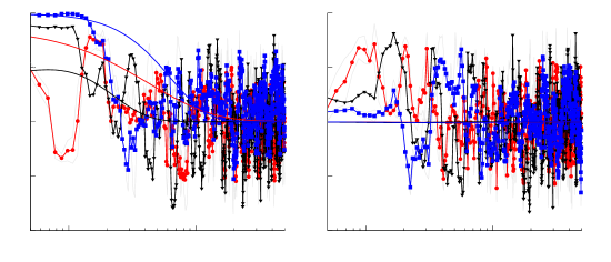
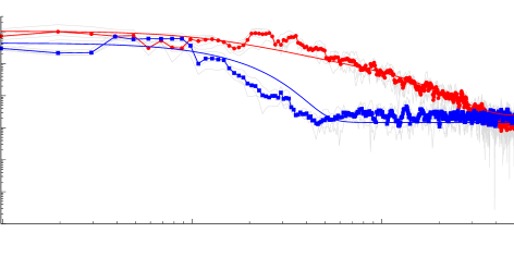
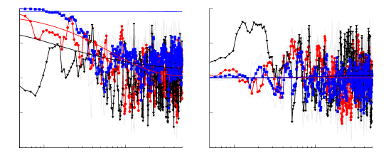
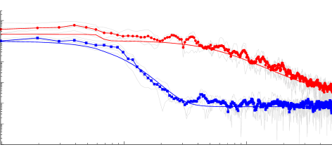
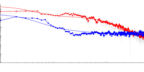
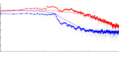
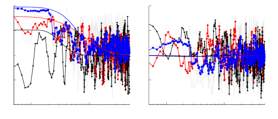
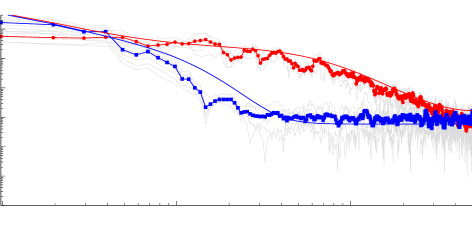
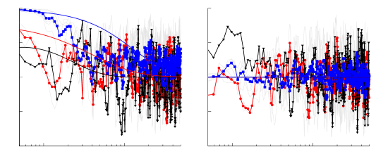
Figures 4 and 5 show the model-implied marginal spectra and coherences for several specific distance respectively, where coherences are shown in terms of their real and imaginary parts. The marginal spectra in general seem well-captured by the model (shown here with the nugget terms added), and the two-regime nonstationarity seems justifiable after inspecting the individual gate spectra that are shown faintly in grey. Maximum likelihood is well-known to prefer capturing high-frequency behavior as accurately as possible over low-frequency behavior, and this observation in an earlier stage of the model formulation was a primary motivator for the extra low-frequency term $(1+B(f))$ in (4.2), which costs a few extra parameters but substantially improves the model’s ability to capture the lowest frequency behavior. It can be seen in the modeled spectra above the ABL that the implied smoothness doesn’t agree as well as it could with the nonparametric estimator. In the supplemental information that shows every figure for all six days, this is a noticeable pattern. To some degree, this is most likely explained by the fact that the likelihood is presumably affected only weakly by changing $S_{x}$ above the ABL in that frequency band and making that parameter slightly incorrect in this marginal sense provided a greater improvement in some other aspect of capturing covariance structure.

Figure 5: Average real (left) and imaginary (right) parts of the complex coherence between measurements three range gates apart above the ABL (blue/squares), below it (red/circles), and twelve gates apart across it (black/triangles), with individual estimators in faint grey. Individual estimates were obtained using multitaper estimators with five sine tapers. Analytical estimates of each part from the MLE are overlaid in lines of the corresponding color.

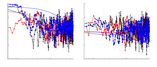
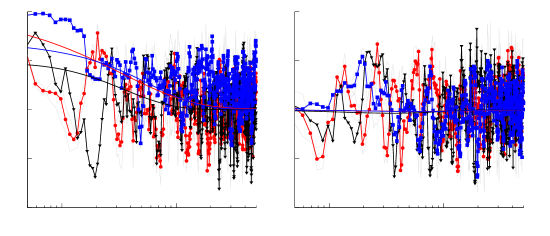
For measurements at this frequency and a reasonably small time segment, coherences are unfortunately very difficult to estimate without either very strong and potentially confounding bias or intractable variability. We attempt to strike a balance between the two in Figure 5, although the interpretation is still difficult. With frequency shown on the log scale, one may be tempted to interpret the imaginary part of the coherence as meaningful, it is quite variable and so it is unsurprising that the model in general suggests that most of the energy of the coherence is in the real part.

&

Figure 6: Side-by-side comparisons of the data used for estimation (above) and a simulation from the GP model with estimated parameters (below), all in units of m/s, for each fitted day.

Bearing in mind that the lowest frequencies are difficult to estimate and so the nonparametric coherence estimators themselves may be suspect, the results suggest that the model is not perfectly specified, in particular above the ABL and in the form of the spatial dependence. In general, the coherence modeling here is more difficult than in Stein (2005b), for example, because of the very high rate of measurements. Noting that these plots again show frequency on the log scale, we see that the coherence estimates are not discernibly different from noise at even relatively low frequencies, and so assessing the quality of the estimated coherence is challening. A slightly more heuristic interpretation of the parametric estimators indicates that the results are plausible, however, in that the MLE does suggest near-unit coherence at low-frequencies above the ABL. While it is tempting to claim that a more complex parametric form might represent these coherences better, inspection of similar figures for other days in the supplementary material suggest that much of what one might interpret to be structure in these estimates does not consistently appear across days, and a more complex form for the coherence might result in overfitting that makes multi-day extensions more challenging, rather than less so.

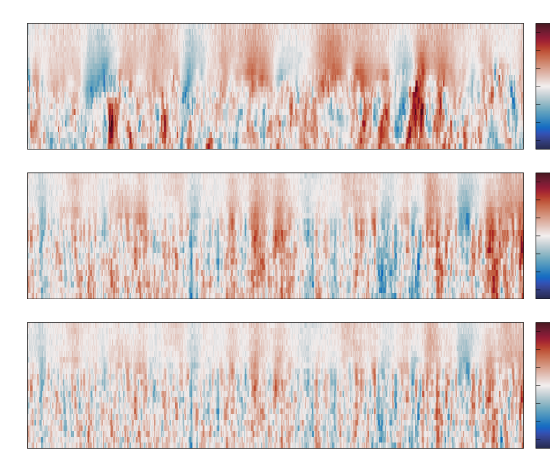
Finally, Figure 4 provides side-by-side cross-section plots (reminiscent of Figure 2) of the measurement data and a simulation from the fitted model for each of the six days. While Table 5 is valuable in assessing the quality of the estimates, for a model of this complexity we also believe that assessing the plausibility of simulations is important. In general, we find the simulations to be satisfying in that regard, although several model mis-specifications are uniquely visible in this format. Interestingly, having a fixed estimator for the ABL height $\beta$ and a smearing-type parameter $\tau$ does seem to effectively create simulations where $\beta$ does not look fixed so long as $\tau$ is relatively small. It does, however, highlight that a fixed $\beta$ means that the estimate will always be near the ABL’s highest point in the data. This makes sense considering that maximum likelihood will certainly penalize under-estimation of uncertainty more harshly than over-estimation. (For example, the likelihood of a $N(0,\sigma=100)$ variable being close to zero is much larger than a $N(0,\sigma=1)$ being close to $100$). The extra variability below the ABL means that the estimate for $\beta$ on June $28$th, for example, is off by as much as $100\text{\,}\mathrm{m}$ from what one might obtain via more sophisticated and targeted methods, for example those of Tucker et al. (2009).

In summary, this model does reasonably well in capturing both quantitative and qualitative features of the process’s covariance structure in the marginal spectra. Moreover, visual assessment of the simulations suggests that at least qualitative features of the coherence are reasonably well-captured. Considering that the quality of the fits and simulations seems reasonably high across all days, we find this to be generally encouraging. See the supplemental material for analogs of all figures shown here for all six of the days studied.

6 Discussion

We have presented here a very flexible modeling framework for regularly measured but nonstationary data. This method provides a convenient and powerful way to think almost exclusively about single-dimension marginal properties of random fields (like spectra and coherences) and obtain fully nonseparable, asymmetric, and nonstationary covariance functions. We are not aware of other methods that are sufficiently flexible that one can specify a $25$-parameter model that composes two different and convenient representations of nonstationarity and for which true maximum likelihood estimation can be performed. On a slightly less significant note, we point out that this method is also uniquely capable of providing estimates for the smoothness $\nu$ and its uncertainty. Derivatives of the modified second-kind Bessel function $\mathcal{K}_{\nu}$ with respect to the smoothness $\nu$ do exist, and there are series expansions that theoretically facilitate computing them (Olver et al. 2010), but we are not aware of any code to do that, and in our own experimentation it is a daunting numerical challenge. In the Fourier domain, however, the derivatives are straightforward. Because of this, the derivative of covariance matrices with respect to $\nu$ are obtained completely analytically, and so there is no need to be concerned with derivative approximations like finite differencing for the kernel function or covariance matrix with respect to $\nu$.

With that said, however, this method of course has drawbacks and is somewhat limited in the way that it can incorporate temporal nonstationarity (or, more generally, nonstationarity in whatever marginal dimension is being transformed over). Further, while some forms of irregularity in time can be mitigated with proper padding and FFT-based interpolation, complete data irregularity—like randomly sampled points—would make this covariance model much more onerous to evaluate. In that sense, we see this method as being complementary to other methods that are more robust in that respect, such as deformation methods (Anderes & Stein 2008) or convolution-based methods (Higdon 2002, Paciorek & Schervish 2006).

The data introduced here—and high-frequency vertical measurements of meteorological processes in general, of which Doppler LIDAR measurements are but one of many—provide a unique opportunity to study space-time random fields. Unlike the well-studied Irish wind data (Haslett & Raftery 1989, Gneiting 2002, Stein 2005a, de Luna & Genton 2005, Horrell & Stein 2017), this data source provides signed measurements at such a high rate in both space and time that it is arguably a different regime in both the relevant atmospheric physics and the relevant statistical concerns. The nonstationarity in altitude—a rarely-considered spatial dimension that is as different from the other two as they all are from time—is sufficiently sharp that there is strong dependence at two altitudes with obviously different marginal behaviors, and thus provides an exceptional testing ground for nonstationary models where they are the most necessary.

With regard to the estimation procedure, it merits consideration that the analytical estimates of the marginal quantities via the MLE are quite different than those obtained via approximate likelihoods, and almost necessarily will look worse visually. In many spectral domain likelihood approximations, one is effectively performing estimation via nonlinear least squares, which is a much more direct attempt at curve fitting. Maximum likelihood, on the other hand, will absolutely sacrifice the very low frequency representation of marginal spectra, for example, if changing such a parameter would increase the likelihood at higher spatio-temporal frequencies. As such, while one should of course expect the estimated quantities $S_{x}$ and $C_{f}$ to be reasonably reflective of marginal spectra and coherences, the estimation procedure itself is not attempting to compartmentalize those quantities or provide the best visual fit of a parametric curve to a nonparametric estimator. In this sense, we find the visual agreement of Figures 4 and 5 to be satisfying, even if a simpler curve-fitting estimation method could likely provide a more impressive visualization.

A major objective of this work was to attempt to write a parametric model that can do a reasonably good job of representing the covariance structure on different days so that eventually those models may be stitched together to form one that is cyclostationary in time on the timescale of weeks. A myriad of other concerns become relevant at that timescale; rain, clouds, and even migratory birds and insect swarms (Muradyan & Coulter 2020) can introduce confounding structure that this model is not adequately equipped to capture. Nonetheless, however, we are encouraged by what has been achieved here, and are hopeful that, going forward, modifications for cyclostationarity will be made possible. One notable concern from the estimation even across just June $2015$, however, is that the day-to-day variation seems high enough that a purely periodic model for many of the parameters (for example $\nu_{1}$) would likely miss a lot of subtle features of the data that are arguably the most interesting, and perhaps most informative about the micrometeorology of the area. A Bayesian perspective may be more appropriate.

More generally, a primary objective for scientists when studying this data is to provide an estimator for the ABL height, which we have denoted as $\beta$. Many works in the meteorological literature provide time series-based methods for estimating this quantity—for example Tucker et al. (2009)—but these methods often do not fully exploit spatio-temporal structure, work on a coarser time scale to provide estimates, and assimilate estimators from multiple data sources. While those estimators are obviously better than the estimate for $\beta$ that is obtained via fitting the model described here, we believe that this work demonstrates that it should be possible to bridge the gap between what the meteorological community does to estimate this quantity and what the spatio-temporal statistics community might do. A Bayesian approach that puts a Matérn-plus-drift prior on the time-varying process $\beta(t)$, for example, might reasonably provide meaningful posterior estimates for the ABL height on the time scale of seconds, as opposed to the time scale of $15$ minutes in Tucker et al. (2009). Moreover, by virtue of being a fully spatio-temporal model, such a procedure could exploit much more structure in the data while also mitigating some potentially non-physical artifacts that occur from estimators that primarily exploit only time dependence, such as large spatial discontinuities. We believe that these and other similar questions are exigent and will likely be fruitful topics of future work.

Government License: The submitted manuscript has been created by UChicago Argonne, LLC, Operator of Argonne National Laboratory (“Argonne”). Argonne, a U.S. Department of Energy Office of Science laboratory, is operated under Contract No. DE-AC02-06CH11357. The U.S. Government retains for itself, and others acting on its behalf, a paid-up nonexclusive, irrevocable worldwide license in said article to reproduce, prepare derivative works, distribute copies to the public, and perform publicly and display publicly, by or on behalf of the Government. The Department of Energy will provide public access to these results of federally sponsored research in accordance with the DOE Public Access Plan. http://energy.gov/downloads/doe-public-access-plan.

Supplementary Material

Figure 7: From top to bottom: The measurements used for fitting on June $03$, a simulation from the full model using fitted parameters, and a simulation from using fitted parameters of a subsetted model with the $\left\{\xi\right\}$ parameters and phase parameter $\alpha$ removed, both using the same random seed. The difference in log-likelihood for all $\approx 17000$ points was only $183$ units, which is a very small per-observation difference. But as can be seen, the difference in visual quality of the simulations is substantial.

Figure 8: Same as Figures 3, 4, and 5 respectively, for June $02$.

Figure 9: Same as Figures 3, 4, and 5 respectively, for June $03$.

Figure 10: Same as Figures 3, 4, and 5 respectively, for June $06$.

Figure 11: Same as Figures 3, 4, and 5 respectively, for June $20$.

Figure 12: Same as Figures 3, 4, and 5 respectively, for June $24$.

Figure 13: Same as Figures 3, 4, and 5 respectively, for June $28$.

References

- (1)
- Anderes & Stein (2008) Anderes, E. B. & Stein, M. L. (2008), ‘Estimating deformations of isotropic Gaussian random fields on the plane’, Annals of Statistics 36(2), 719–741.
- Bezanson et al. (2017) Bezanson, J., Edelman, A., Karpinski, S. & Shah, V. B. (2017), ‘Julia: A fresh approach to numerical computing’, SIAM Review 59(1), 65–98.
- Butterworth (1930) Butterworth, S. (1930), ‘In the theory of filter amplifires’, Experimental Wireless & the Wireless Engineer 7, 536–541.
- Cooley & Tukey (1965) Cooley, J. W. & Tukey, J. W. (1965), ‘An algorithm for the machine calculation of complex Fourier series’, Mathematics of Computation 19(90), 297–301.
- Cressie & Huang (1999) Cressie, N. & Huang, H.-C. (1999), ‘Classes of nonseparable, spatio-temporal stationary covariance functions’, Journal of the American Statistical Association 94(448), 1330–1339.
- Cushman-Roisin (2014) Cushman-Roisin, B. (2014), ‘Atmospheric boundary layer’, Environmental Fluid Mechanics pp. 165–186.
- de Luna & Genton (2005) de Luna, X. & Genton, M. G. (2005), ‘Predictive spatio-temporal models for spatially sparse enviromental data’, Statistica Sinica 15(2), 547–568.
- Fuentes & Smith (2001) Fuentes, M. & Smith, R. (2001), A new class of nonstationary models, Technical report, Tech. report at North Carolina State University, Institute of Statistics.
-
Gage & Balsley (1978)
Gage, K. S. & Balsley, B. B. (1978), ‘Doppler radar probing of the clear atmosphere’, Bulletin of the
American Meteorological Society 59(9), 1074–1094.
https://journals.ametsoc.org/bams/article/59/9/1074/50676/Doppler-Radar-Probing-of-the-Clear-Atmosphere - Genton (2007) Genton, M. G. (2007), ‘Separable approximations of space-time covariance matrices’, Environmetrics 18(7), 681–695.
- Genton & Perrin (2004) Genton, M. G. & Perrin, O. (2004), ‘On a time deformation reducing nonstationary stochastic processes to local stationarity’, Journal of Applied Probability 41(1), 236–249.
- Geoga et al. (2019) Geoga, C. J., Anitescu, M. & Stein, M. L. (2019), ‘Scalable gaussian process computations using hierarchical matrices’, Journal of Computational and Graphical Statistics 0(0), 1–11.
- Gneiting (2002) Gneiting, T. (2002), ‘Nonseparable, stationary covariance functions for space–time data’, Journal of the American Statistical Association 97(458), 590–600.
- Guinness & Stein (2013) Guinness, J. & Stein, M. L. (2013), ‘Interpolation of nonstationary high frequency spatial–temporal temperature data’, Annals of Applied Statistics 7(3), 1684–1708.
- Haslett & Raftery (1989) Haslett, J. & Raftery, A. E. (1989), ‘Space-time modelling with long-memory dependence: assessing ireland’s wind power resource’, Journal of the Royal Statistical Society: Series C (Applied Statistics) 38(1), 1–21.
- Heyde (2008) Heyde, C. C. (2008), Quasi-likelihood and its application: a general approach to optimal parameter estimation, Springer Science & Business Media. Google-Books-ID: forqBwAAQBAJ.
- Higdon (2002) Higdon, D. (2002), Space and space-time modeling using process convolutions, in C. W. Anderson, V. Barnett, P. C. Chatwin & A. H. El-Shaarawi, eds, ‘Quantitative Methods for Current Environmental Issues’, Springer, London, pp. 37–56.
- Horrell & Stein (2017) Horrell, M. T. & Stein, M. L. (2017), ‘Half-spectral space–time covariance models’, Spatial Statistics 19, 90–100.
- Ibragimov & Rozanov (1978) Ibragimov, I. A. & Rozanov, Y. A. (1978), Gaussian random processes, Stochastic Modelling and Applied Probability, Springer-Verlag, New York.
- Jun & Stein (2008) Jun, M. & Stein, M. L. (2008), ‘Nonstationary covariance models for global data’, Annals of Applied Statistics 2(4), 1271–1289.
- Katzfuss (2017) Katzfuss, M. (2017), ‘A multi-resolution approximation for massive spatial datasets’, Journal of the American Statistical Association 112(517), 201–214.
- Katzfuss & Cressie (2012) Katzfuss, M. & Cressie, N. (2012), ‘Bayesian hierarchical spatio-temporal smoothing for very large datasets’, Environmetrics 23(1), 94–107.
- Mather & Voyles (2013) Mather, J. H. & Voyles, J. W. (2013), ‘The arm climate research facility: a review of structure and capabilities’, Bulletin of the American Meteorological Society 94(3), 377–392.
- Matsuo et al. (2011) Matsuo, T., Nychka, D. W. & Paul, D. (2011), ‘Nonstationary covariance modeling for incomplete data: Monte Carlo EM approach’, Computational Statistics & Data Analysis 55(6), 2059–2073.
Muradyan & Coulter (2020)
Muradyan, P. & Coulter, R. (2020),
Radar Wind Profiler (RWP) and Radio Acoustic Sounding
System (RASS) Instrument Handbook (DOE/SC-ARM-TR-044), DOE
Office of Science Atmospheric Radiation Measurement (ARM) Program, United
States.
https://www.arm.gov/publications/tech_reports/handbooks/rwp_handbook.pdf -
Newsom (2012)
Newsom, R. K. (2012), Doppler lidar (Dl)
handbook, Technical Report DOE/SC-ARM/TR-101, DOE Office of Science
Atmospheric Radiation Measurement (ARM) Program (United States).
https://www.osti.gov/biblio/1034640 -
Newsom & Krishnamurthy (2010)
Newsom, R. & Krishnamurthy, R. (2010), Doppler Lidar (DLFPT), Technical report,
Atmospheric Radiation Measurement (ARM) user facility.
doi: 10.5439/1025185.
https://www.archive.arm.gov/metadata/html/sgpdlfptS01.b1.html - Nocedal & Wright (2006) Nocedal, J. & Wright, S. (2006), Numerical optimization, Springer Science & Business Media.
- Nychka et al. (2002) Nychka, D., Wikle, C. & Royle, J. A. (2002), ‘Multiresolution models for nonstationary spatial covariance functions’, Statistical Modelling 2(4), 315–331.
- Olver et al. (2010) Olver, F. W., Lozier, D. W., Boisvert, R. F. & Clark, C. W. (2010), NIST handbook of mathematical functions hardback and CD-ROM, Cambridge university press.
- Paciorek & Schervish (2006) Paciorek, C. J. & Schervish, M. J. (2006), ‘Spatial modelling using a new class of nonstationary covariance functions’, Environmetrics 17(5), 483–506.
- Poppick et al. (2016) Poppick, A., McInerney, D. J., Moyer, E. J. & Stein, M. L. (2016), ‘Temperatures in transient climates: Improved methods for simulations with evolving temporal covariances’, Annals of Applied Statistics 10(1), 477–505.
- Sampson & Guttorp (1992) Sampson, P. D. & Guttorp, P. (1992), ‘Nonparametric estimation of nonstationary spatial covariance structure’, Journal of the American Statistical Association 87(417), 108–119.
- Sisterson et al. (2016) Sisterson, D. L., Peppler, R. A., Cress, T. S., Lamb, P. J. & Turner, D. D. (2016), ‘The arm southern great plains (Sgp) site’, Meteorological Monographs 57, 6.1–6.14.
- Stein (1999) Stein, M. L. (1999), Interpolation of spatial data: some theory for kriging, Springer Science & Business Media.
- Stein (2005a) Stein, M. L. (2005a), Nonstationary spatial covariance functions, Technical report.
- Stein (2005b) Stein, M. L. (2005b), ‘Statistical methods for regular monitoring data’, Journal of the Royal Statistical Society: Series B (Statistical Methodology) 67(5), 667–687.
- Stein et al. (2013) Stein, M. L., Chen, J. & Anitescu, M. (2013), ‘Stochastic approximation of score functions for Gaussian processes’, Annals of Applied Statistics 7(2), 1162–1191.
- Stokes & Schwartz (1994) Stokes, G. M. & Schwartz, S. E. (1994), ‘The atmospheric radiation measurement (Arm) program: programmatic background and design of the cloud and radiation test bed’, Bulletin of the American Meteorological Society 75(7), 1201–1222.
- Tucker et al. (2009) Tucker, S. C., Senff, C. J., Weickmann, A. M., Brewer, W. A., Banta, R. M., Sandberg, S. P., Law, D. C. & Hardesty, R. M. (2009), ‘Doppler lidar estimation of mixing height using turbulence, shear, and aerosol profiles’, Journal of Atmospheric and Oceanic Technology 26(4), 673–688.
- Zhang (2004) Zhang, H. (2004), ‘Inconsistent estimation and asymptotically equal interpolations in model-based geostatistics’, Journal of the American Statistical Association 99(465), 250–261.
- Zhang & Zimmerman (2005) Zhang, H. & Zimmerman, D. L. (2005), ‘Towards reconciling two asymptotic frameworks in spatial statistics’, Biometrika 92(4), 921–936.