Controllable non-Markovianity in phase relaxation

Abstract

Recently remarkable progress in quantum technology has been witnessed. In view of this it is important to investigate an open quantum system as a model of such quantum devices. Quantum devices often require extreme conditions such as very low temperature for the devices to operate. Dynamics can be non-Markovian in such a situation in contrast with Markovian dynamics in high temperature regime. This observation necessitates us to investigate a non-Markovian open quantum system, both theoretically and experimentally. In this paper, we report two important results: 1) Exact solution of a simple but non-trivial theoretical model and 2) demonstration of this model by NMR experiments, where non-Markovianity is continuously controllable. We observe qualitative agreement between theory and experiment.

I Introduction

Quantum resources provide us with novel protocols in several fields in particular in quantum information processing, such as quantum communication, quantum computing and quantum sensing [1]. Many of such protocols have already been demonstrated in actual physical systems thanks to the advance of quantum technology. Since quantum devices suffer from environmental noise, it is important to investigate open quantum systems [2]. Quantum devices are often cooled down to very low temperature to make the devices work. In such situations, the system dynamics often shows non-Markovian behaviour [3, 4, 5, 6, 7] while Markovian one is observed commonly in higher temperature regime. Therefore, it is necessary for us to investigate open quantum systems in various environments theoretically [8, 9, 10] and experimentally [11, 12, 13, 14]. It is, however, generally difficult to experimentally control non-Markovianity of a system dynamics.

Recently, a simple model that showed time-homogeneous, time-inhomogeneous Markovian relaxations and non-Markovian relaxations was proposed in Ref. [15]. The system considered was composed of three subsystems, namely, System I (principal system), Markovian environment and System II inserted between System I and the environment. They analysed the dynamics of this system by solving the Gorini-Kossakowski-Lindblad-Sudarshan (GKLS) master equation [16, 17] analytically. They found that the characteristics of relaxation of System I was controlled by tuning parameters of the environment as well as coupling/decoupling System II with System I. Moreover, they experimentally demonstrated the theoretical results with star-topology molecules in isotropic liquids by using NMR. Through their study, it was found that System II worked as a temporal storage of quantum information that was stored in System I and was dissipating into the Markovian environment.

The coupling between System I and System II in Ref. [15] was simply turned on and off by using an NMR technique called decoupling [18]. It is the purpose of this paper to further extend the model discussed in Ref. [15] by controlling the coupling strength between System I and System II. We analyze this model by solving the GKLS master equation [16, 17] analytically under some reasonable assumptions [19, 20, 21] and compare the theoretical results with those obtained from liquid state NMR experiments. It turns out that our model continuously interpolates between Markovian regime and non-Markovian regime.

The rest of this paper is organized as follows. In Sec. II, we introduce our theoretical model that is made of System I, System II and environment. It is shown that non-Markovianity of the principal system dynamics is controlled by adjusting an external field applied to System II. The dynamics is studied by solving the GKLS equation analytically. We conducted NMR experiments, in which our theoretical model was implemented, and compare theoretical predictions with experimental results in Sec. III. We introduce a quantitative measure of non-Markovianity in our dynamics in Sec. II and compare the theoretical prediction of this measure with experimental results in Sec. III. Section IV is devoted to conclusion and discussion. Details of some derivations are given in Appendix.

II ENGINEERED ENVIRONMENT: THEORY

It is well known that a quantum system relaxes exponentially if it interacts with an environment that has an infinitesimally short memory. This process is called “Markovian”. On the other hand, the relaxation is non-exponential when the system interacts with an environment with a long-time memory. In this case, information of the system temporarily stays in the surrounding environment before it totally dissipates. We call this process “non-Markovian”. There are many studies on Markovian and non-Markovian dynamics; in particular, non-Markovian dynamics is currently attracting much attention [2, 3, 4, 5, 6, 7, 22, 23]. Non-Markovian dynamics often manifests itself in low temperature [3, 4, 5, 6, 7], small size environment, and/or strong coupling regime, for example .

We propose a theoretical model where non-Markovianity of the system dynamics is controlled by adjusting an external field. The first step is to construct an open system that shows non-Markovian dynamics. This is realised by employing the prescription proposed in Ref. [15, 24] as depicted in Fig. 1. System I in Fig. 1 (a) interacts with the environment with a very short-time memory and shows Markovian relaxation. In Fig. 1 (b), System I is surrounded by System II, where two systems interact with each other with a fixed strength. While System II interacts with the Markovian environment, System I interacts with the environment only weakly. Hence the main contribution of the relaxation of System I comes through the interaction with System II. Relaxation of System I in this case can be non-Markovian. System II works as a temporal memory and quantum information escaped from System I is temporarily stored in System II before it totally dissipates into the environment. In other words, System I is in a composite environment (System II and the environment), which has a long-time memory. In the following, we consider a case in which System I is made of one qubit while System II is made of $n~{}(\geq 1)$ identical qubits.

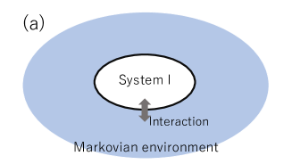
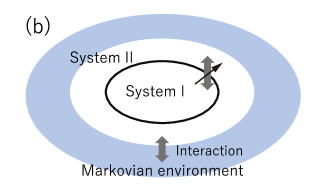
Figure 1: (a) System I interacts with the Markovian environment directly. (b) System I interacts with the Markovian environment indirectly through System II, which results in non-Markovian behaviour in System I. The arrow symbol in the coupling of Systems I and II indicates the coupling strength is effectively variable.

Let us illustrate how to control non-Markovianity before we present detailed calculations. As mentioned before, Systems I and II interact with a fixed strength. However, the coupling strength can be effectively reduced by applying an external field that rotates qubits in System II so that the coupling is partially time-averaged. In the high-field limit, the coupling strength is totally averaged out and System I suffers only from the Markovian environment. In this way, it is possible to interpolates between Markovian and non-Markovian regimes continuously.

II.1 Markovian environment

Let us consider the dynamics of System I of Fig. 1 (a) composed of a single qubit, whose state is given by $\rho$. See also Ref. [15]. Dynamics of the qubit as an open quantum system is governed by the GKLS master equation [2, 16, 17],

$$\frac{d\rho}{dt}=-i[H,\rho]+{\cal L}[\rho],$$ (1)

where $H$ is the Hamiltonian of System I and we call ${\cal L}$ the Lindbladian, which represents the effect of environment. We take $H=0$ here to simplify our analysis. We use the natural unit $\hbar=1$ throughout this paper. The Lindbladian for any completely positive semigroup has the following form [16, 17]:

$${\cal L}[\rho]:=\sum_{i}\gamma_{i}(2L_{i}\rho L^{\dagger}_{i}-\{L_{i}^{\dagger}L_{i},\rho\})$$ (2)

where $\{\gamma_{i}\}$ are positive constants. We consider the case where the environment randomly flip-flops a qubit, in which the explicit form of $\mathcal{L}$ is given by

$${\cal L}[\rho]:=\sum_{\pm}\gamma_{\pm}\left(2\frac{\sigma_{\pm}\rho\sigma_{\mp}}{4}-\left\{\frac{\sigma_{\mp}\sigma_{\pm}}{4},\rho\right\}\right),$$ (3)

where $\sigma_{\pm}=(\sigma_{x}\pm i\sigma_{y})/{2}$ and $\sigma_{k}~{}(k=x,y,z)$ are the Pauli matrices [2]. In this equation, $\gamma_{\pm}$ represents the flip-flop ($|\downarrow\rangle\leftrightarrow|\uparrow\rangle$) rate of the qubit and we assume these rates are symmetric, namely $\gamma_{+}=\gamma_{-}:=\gamma_{\rm I}$.

Now GKLS equation is given by

$$\frac{d\rho}{dt}=\sum_{\pm}\gamma_{\rm I}\left(2\frac{\sigma_{\pm}\rho\sigma_{\mp}}{4}-\left\{\frac{\sigma_{\mp}\sigma_{\pm}}{4},\rho\right\}\right).$$ (4)

It is shown that Eq. (4) is solved exactly leading to exponential relaxation with a characteristic time $2/\gamma_{\rm I}$.

II.2 Non-Markovian environment: $(1+1)$-qubit case

We now introduce a theoretical model, in which non-Markovianity can be continuously controlled by an external field. First, we consider the simplest case where both Systems I and II consist of a single qubit, which we call the $(1+1)$-system. The System I qubit has an index 0 while the System II qubit has an index 1. The density matrix $\rho^{(1)}$ of the total system is given by

$$\rho^{(1)}=\frac{1}{2}\begin{pmatrix}\rho_{11}&\rho_{12}&\rho_{13}&\rho_{14}\\ \rho^{*}_{12}&\rho_{22}&\rho_{23}&\rho_{24}\\ \rho^{*}_{13}&\rho^{*}_{23}&\rho_{33}&\rho_{34}\\ \rho^{*}_{14}&\rho^{*}_{24}&\rho^{*}_{34}&\rho_{44}\\ \end{pmatrix}.$$ (5)

Here the basis vectors are ordered as $\{|00\rangle,|01\rangle,|10\rangle,|11\rangle\}$ with $|ab\rangle=|a\rangle_{0}\otimes|b\rangle_{1},\ a,b\in\{0,1\}$. Each qubit in this system is subject to the flip-flop noise independently. The Lindbladian in this case is given by

$${\cal L}[\rho^{(1)}]=\sum_{i={\rm 0,1}}\sum_{\pm}\gamma_{i}\left(2\frac{\sigma^{(i)}_{\pm}\rho^{(1)}\sigma^{(i)}_{\mp}}{4}-\left\{\frac{\sigma^{(i)}_{\mp}\sigma^{(i)}_{\pm}}{4},\rho^{(1)}\right\}\right):=\sum_{i={\rm 0,1}}{\cal L}^{(i)}[\rho^{(1)}],$$ (6)

where $\sigma^{(i)}_{\mu}$ is the $\mu$-component of the Pauli matrices acting non-trivially only on the $i$-th qubit, i.e., $\sigma^{(0)}_{\mu}=\sigma_{\mu}\otimes\sigma_{0}$, $\sigma^{(1)}_{\mu}=\sigma_{0}\otimes\sigma_{\mu}$ and $\sigma^{(i)}_{\pm}={\sigma^{(i)}_{x}\pm i\sigma^{(i)}_{y}}/{2}$ and $\sigma_{0}$ is the $2\times 2$ identity matrix. Here $\gamma_{i}$ is the flip-flop rate of the $i$-th qubit. $\gamma_{0}(\gamma_{1})$ is also called $\gamma_{\rm I}(\gamma_{\rm II})$ because the $\gamma_{0}(\gamma_{1})$ is the flip-flop rate of the qubit in System I (II). Suppose the Hamiltonian of the total system is given by

$$H^{(1)}=H_{J}^{(1)}+H_{\omega_{1}}^{(1)},H_{J}^{(1)}:=J\frac{\sigma^{(0)}_{z}\sigma^{(1)}_{z}}{4},H_{\omega_{1}}^{(1)}:=\omega_{1}\frac{\sigma^{(1)}_{x}}{2}.$$ (7)

$H_{J}^{(1)}$ is a qubit-qubit interaction with a constant strength $J$, while $H_{\omega_{1}}^{(1)}$ represents a controllable external field $\omega_{1}$ coupled to the $x$-component of the System II qubit.

The dynamics of this system is governed by the GKLS master equation,

$$\frac{d\rho^{(1)}}{dt} =-i[H^{(1)},\rho^{(1)}]+{\cal L}[\rho^{(1)}]={\cal D}^{(1)}[\rho^{(1)}]+{\cal L}^{(0)}[\rho^{(1)}],$$

$${\cal D}^{(1)}[\bullet] :=-i\left[H^{(1)},~{}\bullet~{}\right]+{\cal L}^{(1)}[\bullet].$$ (8)

Let us write the density matrix $\rho^{(1)}$ in the following form:

$$\rho^{(1)}=\frac{\sigma^{(0)}_{0}}{2}\cdot\frac{A_{1}^{(1)}+A_{2}^{(1)}}{2}+\frac{\sigma^{(0)}_{z}}{2}\cdot\frac{A_{1}^{(1)}-A_{2}^{(1)}}{2}+\frac{\sigma^{(0)}_{+}}{2}\cdot B^{(1)}+\frac{\sigma^{(0)}_{-}}{2}\cdot(B^{(1)})^{\dagger},$$ (9)

where

$$A_{1}^{(1)}:=\sigma_{0}\otimes\begin{pmatrix}\rho_{11}&\rho_{12}\\ \rho^{*}_{12}&\rho_{22}\end{pmatrix},~{}A_{2}^{(1)}:=\sigma_{0}\otimes\begin{pmatrix}\rho_{33}&\rho_{34}\\ \rho^{*}_{34}&\rho_{44}\end{pmatrix},~{}B^{(1)}:=\sigma_{0}\otimes\begin{pmatrix}\rho_{13}&\rho_{14}\\ \rho_{23}&\rho_{24}\end{pmatrix}.$$ (10)

We easily find that Eq. (8) is decomposed into the following four equations,

$$\frac{dA_{1}^{(1)}}{dt}=f(A_{1}^{(1)},A_{2}^{(1)}),~{}\frac{dA_{2}^{(1)}}{dt}=g(A_{1}^{(1)},A_{2}^{(1)}),~{}\frac{dB^{(1)}}{dt}=h(B^{(1)}),~{}\frac{d(B^{(1)})^{\dagger}}{dt}=[h(B^{(1)})]^{\dagger}.$$ (11)

An important observation is that the dynamics of $B^{(1)}$ is decoupled from those of $A_{1}^{(1)}$, $A_{2}^{(1)}$ and $(B^{(1)})^{\dagger}$.

Now we solve Eq. (11) with an appropriate initial condition. Suppose qubit 0 is polarized along the $x$ axis and qubit 1 is uniformly mixed at $t=0$;

$$\rho^{(1)}(0)=|+\rangle\langle+|\otimes\frac{1}{2}\sigma_{0}=\frac{1}{2\cdot 2}\begin{pmatrix}1&0&1&0\\ 0&1&0&1\\ 1&0&1&0\\ 0&1&0&1\end{pmatrix},$$ (12)

where $|+\rangle=\frac{1}{\sqrt{2}}(|0\rangle+|1\rangle)$. This initial condition is rewritten as

$$A_{1}^{(1)}(0)=A_{2}^{(1)}(0)=B^{(1)}(0)=(B^{(1)})^{\dagger}(0)=\sigma_{0}\otimes\frac{1}{2}\sigma_{0}.$$ (13)

Then it turns out that the first two equations in Eq. (11) have no dynamics: $f(A_{1}^{(1)},A_{2}^{(1)})=g(A_{1}^{(1)},A_{2}^{(1)})=0$ at any $t$. In other words, $A_{1}^{(1)}$ and $A_{2}^{(1)}$ are time-independent with this initial condition. As a result we only need to solve ${dB^{(1)}}/{dt}=h(B^{(1)})$ to find the dynamics of the GKLS equation. To write down the dynamical equation of $B^{(1)}$, we now evaluate the GKLS equation on $\frac{1}{2}\sigma^{(0)}_{+}\cdot B^{(1)}$. First note that ${\cal L}^{(0)}$ acts only on $\sigma^{(0)}_{+}$ and gives just a scalar multiplication:

$${\cal L}^{(0)}\left[\frac{\sigma^{\rm I}_{+}}{2}\cdot B^{(1)}\right]=-\Bigl{(}\frac{\gamma_{\rm I}}{2}\cdot\frac{\sigma^{(0)}_{+}}{2}\Bigr{)}\cdot B^{(1)}.$$ (14)

This implies that $B^{(1)}$ is factorised as $B^{(1)}=e^{-\gamma_{\rm I}t/2}\tilde{B}^{(1)}$. The dynamics of $\tilde{B}^{(1)}$ following from the GKLS equation (8) is written as

$$\frac{d}{dt}\Bigl{(}\frac{\sigma_{+}^{(0)}}{2}\cdot\tilde{B}^{(1)}\Bigr{)}={\cal D}^{(1)}\left[\frac{\sigma_{+}^{(0)}}{2}\cdot\tilde{B}^{(1)}\right].$$ (15)

The dynamics of $B^{(1)}$ can be obtained by multiplying $e^{-\gamma_{\rm I}t/2}$ to $\tilde{B}^{(1)}$ (or, $B^{(1)}$ with $\gamma_{\rm I}=0$). Therefore, we will consider the case when $\gamma_{\rm I}=0$ hereafter.

$\tilde{B}^{(1)}$ can be expanded as $\tilde{B}^{(1)}=\frac{1}{2}\sum_{k=0,x,y,z}b_{k}\sigma^{(1)}_{k}$, where

$$b_{0}=\rho_{13}+\rho_{24},~{}b_{x}=\rho_{14}+\rho_{23},~{}b_{y}=i(\rho_{14}-\rho_{23}),~{}b_{z}=\rho_{13}-\rho_{24}.$$

We now evaluate the right-hand side of Eq. (15). The action on each basis $\frac{1}{2}\sigma^{(0)}_{+}\cdot(\sigma^{(1)}_{k}/2)$ of $\frac{1}{2}\sigma^{(0)}_{+}\cdot\tilde{B}^{(1)}$ is given as

$${\cal D}^{(1)}\left[\frac{\sigma_{+}^{(0)}}{2}\cdot\frac{\sigma^{(1)}_{0}}{2}\right] =-i\frac{J}{2}\Bigl{(}\frac{\sigma_{+}^{(0)}}{2}\cdot\frac{\sigma^{(1)}_{z}}{2}\Bigr{)},$$

$${\cal D}^{(1)}\left[\frac{\sigma_{+}^{(0)}}{2}\cdot\frac{\sigma^{(1)}_{x}}{2}\right] =-\frac{\gamma_{\rm II}}{2}\Bigl{(}\frac{\sigma_{+}^{(0)}}{2}\cdot\frac{\sigma^{(1)}_{x}}{2}\Bigr{)},$$

$${\cal D}^{(1)}\left[\frac{\sigma_{+}^{(0)}}{2}\cdot\frac{\sigma^{(1)}_{y}}{2}\right] =\omega_{1}\Bigl{(}\frac{\sigma_{+}^{(0)}}{2}\cdot\frac{\sigma^{(1)}_{z}}{2}\Bigr{)}-\frac{\gamma_{\rm II}}{2}\Bigl{(}\frac{\sigma_{+}^{(0)}}{2}\cdot\frac{\sigma^{(1)}_{y}}{2}\Bigr{)},$$

$${\cal D}^{(1)}\left[\frac{\sigma_{+}^{(0)}}{2}\cdot\frac{\sigma^{(1)}_{z}}{2}\right] =-i\frac{J}{2}\Bigl{(}\frac{\sigma_{+}^{(0)}}{2}\cdot\frac{\sigma^{(1)}_{0}}{2}\Bigr{)}-\gamma_{\rm II}\Bigl{(}\frac{\sigma_{+}^{(0)}}{2}\cdot\frac{\sigma^{(1)}_{z}}{2}\Bigr{)}-\omega_{1}\Bigl{(}\frac{\sigma_{+}^{(0)}}{2}\cdot\frac{\sigma^{(1)}_{y}}{2}\Bigr{)}.$$ (16)

We summarise the action of ${\cal D}^{(1)}$ on $\frac{1}{2}\sigma_{+}^{(0)}\cdot\tilde{B}^{(1)}$ as

$${\cal D}^{(1)}\left[\frac{\sigma_{+}^{(0)}}{2}\cdot\tilde{B}^{(1)}\right]=\frac{\sigma_{+}^{(0)}}{2}\cdot\sum_{k,m=0,x,y,z}b_{k}({\mathbb{M}}_{0})_{km}\frac{\sigma^{(i)}_{m}}{2},$$ (17)

where

$${\mathbb{M}_{0}}:=\frac{1}{2}\begin{matrix}0~{}~{}~{}~{}~{}x~{}~{}~{}~{}~{}~{}y~{}~{}~{}~{}~{}~{}z\\ \begin{pmatrix}0&0&0&-iJ\\ 0&-\gamma_{\rm II}&0&0\\ 0&0&-\gamma_{\rm II}&2\omega_{1}\\ -iJ&0&-2\omega_{1}&-2\gamma_{\rm II}\end{pmatrix}.\end{matrix}$$ (18)

Comparing the coefficients of each basis $\frac{1}{2}\sigma^{(0)}_{+}\cdot(\sigma^{(1)}_{k}/2)$ in the left-hand side and the right-hand side of Eq. (15), we obtain the following differential equations for $b_{k}$:

$$\frac{d}{dt}\begin{pmatrix}b_{0}\\ b_{x}\\ b_{y}\\ b_{z}\end{pmatrix}={\mathbb{M}_{0}}^{\rm T}\begin{pmatrix}b_{0}\\ b_{x}\\ b_{y}\\ b_{z}\end{pmatrix}.$$ (19)

Note that the dynamics of $b_{x}$ is totally decoupled from the other variables. Hereafter, we ignore the dynamics of $b_{x}$ by employing the initial condition (13), that is, $b_{0}(0)=1$ and $b_{x}(0)=b_{y}(0)=b_{z}(0)=0$. The remaining equations are concisely written in the following matrix form:

$$\frac{d}{dt}\begin{pmatrix}b_{0}\\ b_{y}\\ b_{z}\end{pmatrix}={\mathbb{M}}^{\rm T}\begin{pmatrix}b_{0}\\ b_{y}\\ b_{z}\end{pmatrix},$$ (20)

where

$${\mathbb{M}}:=\frac{1}{2}\begin{pmatrix}0&0&-iJ\\ 0&-\gamma_{\rm II}&2\omega_{1}\\ -iJ&-2\omega_{1}&-2\gamma_{\rm II}\end{pmatrix}.$$ (21)

This equation is analytically solvable since $\mathbf{M}$ is constant and its eigenvalues and eigenvectors are easily found (See Appendix A).

Let us evaluate the reduced density matrix of System I, $\rho_{\rm I}^{(1)}$ by tracing out System II with the initial condition (13). After straightforward calculation, we obtain

$$\rho^{(1)}_{{\mathrm{I}}}={\rm Tr_{II}}(\rho^{(1)})=\frac{1}{2}\begin{pmatrix}1&e^{-\gamma_{\rm I}t/2}b_{0}(t)\\ e^{-\gamma_{\rm I}t/2}b_{0}(t)&1\end{pmatrix}.$$ (22)

The explicit form of $b_{0}(t)$ is given in Appendix A, where we also show that $b_{0}(t)$ is real. Note that $\rho^{(1)}_{{\mathrm{I}}}(0)=|+\rangle\langle+|$ and $\rho^{(1)}_{{\mathrm{I}}}(\infty)=\sigma_{0}/2$.

II.3 Non-Markovian environment: $(1+n)$-qubit case

The above analysis is readily generalised to the case where System II consists of $n$ identical qubits. We call this system the $(1+n)$-system [15]. We consider a system in which the System I qubit interacts with all System II qubits with equal coupling strength $J$ while the qubits in System II do not interact among themselves. Moreover, there is an external field $\omega_{1}$ that couples equally with all the System II qubits. The Hamiltonian of this system is then given by

$$H=\sum^{n}_{i=1}\left(H^{(i)}_{J}+H^{(i)}_{\omega_{1}}\right),\ H^{(i)}_{J}:=J\frac{\sigma^{(0)}_{z}\sigma^{(i)}_{z}}{4},\ H^{(i)}_{\omega_{1}}:=\omega_{1}\frac{\sigma^{(i)}_{x}}{2},$$ (23)

where $\sigma_{\mu}^{(i)}=\sigma_{0}\otimes\ldots\otimes\sigma_{0}\otimes\sigma_{\mu}\otimes\sigma_{0}\otimes\ldots\otimes\sigma_{0}$ nontrivially acts only on the $i$-th qubit. Here we assign an index 0 to the System I qubit while indices 1 to $n$ to the System II qubits. The basis vectors are ordered as

$$\{|00\ldots 00\rangle,|00\ldots 01\rangle,|00\ldots 11\rangle,\ldots,|11\ldots 10\rangle,|11\ldots 11\rangle\},$$ (24)

where $|ab\ldots cd\rangle=|a\rangle_{0}\otimes|b\rangle_{1}\otimes\ldots\otimes|c\rangle_{n-1}\otimes|d\rangle_{n}$.

The Lindbladian which represents the flip-flop noise that acts on all qubits independently is

$${\cal L}[\rho]=\sum^{n}_{i=0}\sum_{\pm}\gamma_{i}\left(2\frac{\sigma^{(i)}_{\pm}\rho\sigma^{(i)}_{\mp}}{4}-\left\{\frac{\sigma^{(i)}_{\mp}\sigma^{(i)}_{\pm}}{4},\rho\right\}\right):=\sum^{n}_{i=0}{\cal L}^{(i)}[\rho].$$ (25)

We assume from now on that the strength $\gamma_{i}$ for all the qubits in System II are identical: $\gamma_{1}=\gamma_{2}=\ldots=\gamma_{n}=:\gamma_{\rm II}$.

The dynamics of the density matrix $\rho^{(n)}$ of Systems I and II is described by

$$\frac{d\rho^{(n)}}{dt} =-i[H,\rho^{(n)}]+{\cal L}[\rho^{(n)}]=\sum^{n}_{i=1}{\cal D}^{(i)}[\rho^{(n)}]+{\cal L}^{(0)}[\rho^{(n)}],$$

$${\cal D}^{(i)}[\bullet] :=-i\left[(H^{(i)}_{J}+H^{(i)}_{\omega_{1}}),~{}\bullet~{}\right]+{\cal L}^{(i)}[\bullet].$$ (26)

Let us write $\rho^{(n)}$ in the same form as the $(1+1)$-case,

$$\rho^{(n)}=\frac{\sigma^{(0)}_{0}}{2}\cdot\frac{A_{1}^{(n)}+A_{2}^{(n)}}{2}+\frac{\sigma^{(0)}_{z}}{2}\cdot\frac{A_{1}^{(n)}-A_{2}^{(n)}}{2}+\frac{\sigma^{(0)}_{+}}{2}\cdot B^{(n)}+\frac{\sigma^{(0)}_{-}}{2}\cdot(B^{(n)})^{\dagger}.$$ (27)

$A_{1}^{(n)}$, $A_{2}^{(n)}$ and $B^{(n)}$ respectively have matrix forms $\sigma_{0}\otimes{A_{1}^{\prime}}^{(n)}$, $\sigma_{0}\otimes{A^{\prime}_{2}}^{(n)}$ and $\sigma_{0}\otimes{B^{\prime}}^{(n)}$ where ${A^{\prime}_{1}}^{(n)}$, ${A^{\prime}_{2}}^{(n)}$ and ${B^{\prime}}^{(n)}$ are $2^{n}\times 2^{n}$ matrices. Equivalently, $\rho^{(n)}$ can be represented by the following block matrix form:

$$\rho^{(n)}=\begin{pmatrix}{A^{\prime}_{1}}^{(n)}&{B^{\prime}}^{(n)}\\ ({B^{\prime}}^{(n)})^{\dagger}&{A^{\prime}_{2}}^{(n)}\end{pmatrix}.$$ (28)

We can find that the dynamics of $B^{(n)}$ is decoupled from those of $A_{1}^{(n)}$, $A_{2}^{(n)}$ and $(B^{(n)})^{\dagger}$ as in the (1+1)-case. We are interested in the initial state

$$\rho^{(n)}(0)=|+\rangle\langle+|\otimes(\frac{1}{2}\sigma_{0})^{\otimes n}=\frac{1}{2^{n+1}}\begin{pmatrix}\sigma^{\otimes n}_{0}&\sigma^{\otimes n}_{0}\\ \sigma^{\otimes n}_{0}&\sigma^{\otimes n}_{0}\end{pmatrix},$$ (29)

which is a generalisation of Eq. (12) for the $(1+1)$-system to the $(1+n)$-system. This initial condition in terms of $A_{1}^{(n)},A_{2}^{(n)},B^{(n)}$ and $(B^{(n)})^{\dagger}$ is

$$A_{1}^{(n)}(0)=A_{2}^{(n)}(0)=B^{(n)}(0)=(B^{(n)})^{\dagger}(0)=\sigma_{0}\otimes\frac{1}{2^{n}}\sigma^{\otimes n}_{0}\qquad(t\geq 0)$$ (30)

Solutions of $A_{1}^{(n)}$ and $A_{2}^{(n)}$ are time independent with this initial condition.

Since the action of ${\cal L}^{(0)}$ gives just a scalar multiplication as mentioned previously, we find that the GKLS equation (26) can be rewritten as

$$\frac{d}{dt}\Bigl{(}\frac{\sigma_{+}^{(0)}}{2}\cdot\tilde{B}^{(n)}\Bigr{)}=\sum^{n}_{i=1}{\cal D}^{(i)}\left[\frac{\sigma_{+}^{(0)}}{2}\cdot\tilde{B}^{(n)}\right],$$ (31)

where $\tilde{B}^{(n)}:=e^{-\gamma_{\rm I}t/2}B^{(n)}$. We write

$$\tilde{B}^{(n)}=\prod^{n}_{i=1}\varsigma^{(i)}$$ (32)

where

$$\varsigma^{(i)}=\frac{1}{2}\sum_{k=0,x,y,z}b^{(i)}_{k}\sigma_{k}^{(i)}$$ (33)

with $b^{(i)}_{k}\in\mathbb{C}$. Our initial condition gives $b^{(i)}_{0}(0)=1,b^{(i)}_{x}(0)=b^{(i)}_{y}(0)=b^{(i)}_{z}(0)=0$ where $1\leq i\leq n$. It turns out that $b^{(i)}_{x}$ decouples from the dynamics of the other $b^{(i)}_{k}$’s and we can set $b^{(i)}_{x}(t)=0$ from the given initial condition. It follows from Eq. (32) that the density matrix $\rho^{(n)}$ correctly reflects the symmetry under arbitrary permutation of $n$ qubits in System II and that there are no correlations among them.

We then calculate the action of ${\cal D}^{(i)}$. Since ${\cal D}^{(i)}$ acts only on the $0$-th and $i$-th qubits, it sufficies to consider the term $\frac{1}{2}\sigma_{+}^{(0)}\cdot\varsigma^{(i)}$ only. The action of ${\cal D}^{(i)}$ on $\frac{1}{2}\sigma_{+}^{(0)}\cdot({\sigma^{(i)}_{\mu}}/{2})$ is given as

$${\cal D}^{(i)}\left[\frac{\sigma_{+}^{(0)}}{2}\cdot\frac{\sigma^{(i)}_{0}}{2}\right] =-i\frac{J}{2}\Bigl{(}\frac{\sigma_{+}^{(0)}}{2}\cdot\frac{\sigma^{(i)}_{z}}{2}\Bigr{)},$$

$${\cal D}^{(i)}\left[\frac{\sigma_{+}^{(0)}}{2}\cdot\frac{\sigma^{(i)}_{y}}{2}\right] =\omega_{1}\Bigl{(}\frac{\sigma_{+}^{(0)}}{2}\cdot\frac{\sigma^{(i)}_{z}}{2}\Bigr{)}-\frac{\gamma_{\rm II}}{2}\Bigl{(}\frac{\sigma_{+}^{(0)}}{2}\cdot\frac{\sigma^{(i)}_{y}}{2}\Bigr{)},$$

$${\cal D}^{(i)}\left[\frac{\sigma_{+}^{(0)}}{2}\cdot\frac{\sigma^{(i)}_{z}}{2}\right] =-i\frac{J}{2}\Bigl{(}\frac{\sigma_{+}^{(0)}}{2}\cdot\frac{\sigma^{(i)}_{0}}{2}\Bigr{)}-\gamma_{\rm II}\Bigl{(}\frac{\sigma_{+}^{(0)}}{2}\cdot\frac{\sigma^{(i)}_{z}}{2}\Bigr{)}-\omega_{1}\Bigl{(}\frac{\sigma_{+}^{(0)}}{2}\cdot\frac{\sigma^{(i)}_{y}}{2}\Bigr{)}.$$ (34)

We summarise the action of ${\cal D}^{(i)}$ on $\frac{\sigma_{+}^{(0)}}{2}\cdot\varsigma^{(i)}$ as

$${\cal D}^{(i)}\left[\frac{\sigma_{+}^{(0)}}{2}\cdot\varsigma^{(i)}\right]=\frac{\sigma_{+}^{(0)}}{2}\cdot\sum_{k,m=0,y,z}b^{(i)}_{k}({\mathbb{M}})_{km}\frac{\sigma^{(i)}_{m}}{2},$$ (35)

where

$${\mathbb{M}}=\frac{1}{2}\begin{matrix}0~{}~{}~{}~{}~{}y~{}~{}~{}~{}~{}z\\ \begin{pmatrix}0&0&-iJ\\ 0&-\gamma_{\rm II}&2\omega_{1}\\ -iJ&-2\omega_{1}&-2\gamma_{\rm II}\end{pmatrix}\end{matrix},$$ (36)

which is the same ${\mathbb{M}}$ introduced in the $(1+1)$-system. The dynamics of $\tilde{B}^{(n)}$ following from Eq. (31) is written as

$$\frac{d}{dt}\Bigl{(}\frac{\sigma_{+}^{(0)}}{2}\cdot \prod^{n}_{i=1}\varsigma^{(i)}\Bigr{)}=\sum^{n}_{i=1}{\cal D}^{(i)}\left[\frac{\sigma_{+}^{(0)}}{2}\cdot\Bigl{(}\prod^{n}_{i=1}\varsigma^{(i)}\Bigr{)}\right]$$

$$= \frac{\sigma_{+}^{(0)}}{2}\cdot\left[\Bigl{(}\sum_{k,m=0,y,z}b^{(1)}_{k}({\mathbb{M}})_{km}\frac{\sigma^{(1)}_{m}}{2}\Bigr{)}\cdot\varsigma^{(2)}\cdot\ldots\cdot\varsigma^{(i)}\cdot\ldots\cdot\varsigma^{(n)}\right]+\ldots$$

$$+\ldots+\frac{\sigma_{+}^{(0)}}{2}\cdot\left[\varsigma^{(1)}\cdot\ldots\cdot\Bigl{(}\sum_{k,m=0,y,z}b^{(i)}_{k}({\mathbb{M}})_{km}\frac{\sigma^{(i)}_{m}}{2}\Bigr{)}\cdot\ldots\cdot\varsigma^{(n)}\right]$$

$$+\ldots+\frac{\sigma_{+}^{(0)}}{2}\cdot\left[\varsigma^{(1)}\cdot\ldots\cdot\varsigma^{(i)}\cdot\ldots\cdot\Bigl{(}\sum_{k,m=0,y,z}b^{(n)}_{k}({\mathbb{M}})_{km}\frac{\sigma^{(n)}_{m}}{2}\Bigr{)}\right].$$ (37)

Comparing the coefficients of each basis in the left-hand side and the right-hand side, we obtain differential equations for each coefficient $b^{(1)}_{k}\ldots b^{(i)}_{k}\ldots b^{(n)}_{k}$ as

$$\frac{d}{dt}(b^{(1)}_{k}\ldots b^{(i)}_{k}\ldots b^{(n)}_{k})= \Bigl{(}\sum_{m=0,y,z}({\mathbb{M}}^{\rm T})_{km}b^{(1)}_{m}\Bigr{)}b^{(2)}_{k}\ldots b^{(i)}_{k}\ldots b^{(n)}_{k}+\ldots$$

$$+ b^{(1)}_{k}\ldots b^{(i-1)}_{k}\Bigl{(}\sum_{m=0,y,z}({\mathbb{M}}^{\rm T})_{km}b^{(i)}_{m}\Bigr{)}b^{(i+1)}_{k}\ldots b^{(n)}_{k}+\ldots$$

$$+ b^{(1)}_{k}\ldots b^{(i)}_{k}\ldots b^{(n-1)}_{k}\Bigl{(}\sum_{m=0,y,z}({\mathbb{M}}^{\rm T})_{km}b^{(n)}_{m}\Bigr{)}.$$ (38)

We rewrite this equation as

$$\Bigl{(}\frac{db^{(1)}_{k}}{dt}-\sum_{m=0,y,z}({\mathbb{M}}^{\rm T})_{km}b^{(1)}_{m}\Bigr{)}b^{(2)}_{k}\ldots b^{(i)}_{k}\ldots b^{(n)}_{k}+\ldots$$

$$+ b^{(1)}_{k}\ldots b^{(i-1)}_{k}\Bigl{(}\frac{db^{(i)}_{k}}{dt}-\sum_{m=0,y,z}({\mathbb{M}}^{\rm T})_{km}b^{(i)}_{m}\Bigr{)}b^{(i+1)}_{k}\ldots b^{(n)}_{k}+\ldots$$

$$+ b^{(1)}_{k}\ldots b^{(i)}_{k}\ldots b^{(n-1)}_{k}\Bigl{(}\frac{db^{(n)}_{k}}{dt}-\sum_{m=0,y,z}({\mathbb{M}}^{\rm T})_{km}b^{(n)}_{m}\Bigr{)}=0.$$ (39)

We obtain the differential equations

$$\frac{d}{dt}\begin{pmatrix}b^{(i)}_{0}\\ b^{(i)}_{y}\\ b^{(i)}_{z}\end{pmatrix}={\mathbb{M}}^{\rm T}\begin{pmatrix}b^{(i)}_{0}\\ b^{(i)}_{y}\\ b^{(i)}_{z}\end{pmatrix},\qquad 1\leq i\leq n.$$ (40)

Note that these differential equations are the same as Eq. (20) in the $(1+1)$-system. Moreover, the initial conditions are the same for all $i$ and thus the dynamics is solvable for any $n$ by employing $b_{0}(t)$ obtained for the (1+1)-system. This solution is reasonable because the qubits in System II are identical.

Let us evaluate the reduced density matrix $\rho_{\rm I}^{(n)}$ of System I, by tracing out System II. Note that ${\rm Tr}(\varsigma^{(i)})=b_{0}$ since Pauli matrices are traceless. We obtain

$$\rho^{(n)}_{\mathrm{I}}(t):={\rm Tr}_{\rm II}\,\rho^{(n)}= \frac{\sigma^{(0)}_{0}}{2}\cdot{\rm Tr}\left(\prod^{n}_{i=1}\frac{\sigma^{(i)}_{0}}{2}\right)+e^{-\gamma_{\rm I}t/2}\left[\frac{\sigma^{(0)}_{+}}{2}\cdot{\rm Tr}\left(\prod^{n}_{i=1}\varsigma^{(i)}\right)+\mbox{h.c.}\right]$$

$$= \frac{\sigma^{(0)}_{0}}{2}+e^{-\gamma_{\rm I}t/2}\left(\frac{\sigma^{(0)}_{+}}{2}b_{0}^{n}+\mbox{h.c.}\right)$$

$$= \frac{1}{2}\begin{pmatrix}1&e^{-\gamma_{\rm I}t/2}\left(b_{0}(t)\right)^{n}\\ e^{-\gamma_{\rm I}t/2}\left(b_{0}(t)\right)^{n}&1\end{pmatrix}.$$ (41)

We find that the effect of the direct coupling of the Markovian environment with System I, shown as the factor of $e^{-\gamma_{\rm I}t/2}$, is well separated from those through System II, which is the origin of the non-Markovian dynamics of System I. We introduce

$$\beta_{n}(t):=e^{-\gamma_{\rm I}t/2}(b_{0}(t))^{n}$$ (42)

for later convenience.

One might think that our model is a trivial extension of one introduced in Ref. [15] since the only difference is the existence of the external field $\omega_{1}$. However, $H_{\omega_{1}}^{(i)}$ does not commute with $H_{J}^{(i)}$, which makes our solution highly non-trivial compared to that obtained in Ref. [15]. Moreover, the dynamics of our model has three degrees of freedom, while that of Ref. [15] has only two degrees of freedom. As a result, this model shows drastically different behaviours from the previous one. It is possible to control non-Markovianity of the dynamics continuously by changing the external field strength $\omega_{1}$ as will be shown in Sec. III.

II.4 Non-Markovianity measure

We will discuss control of non-Markovianity of dynamics by manipulating an external field in Sec. III. To this end, let us first introduce a measure ${\cal N}$ to quantify non-Markovianity of dynamics. We employ the measure proposed in [25], which is based on the concept of information backflow from the environment. This measure is described in terms of the trace distance $D[\rho(t),\rho^{\prime}(t)]={\rm Tr}|\rho(t)-\rho^{\prime}(t)|/2$ between two states $\rho$ and $\rho^{\prime}$ of a system of interest. Note that the environmental freedoms are traced out here. ${\cal N}$ introduced in [25] is defined as

$${\cal N}:=\max_{\rho(0),\rho^{\prime}(0)}\int_{\Omega_{+}}\frac{dD[\rho(t),\rho^{\prime}(t)]}{dt}dt,$$ (43)

where $\Omega_{+}:=\{t\in[0,\infty)|dD[\rho(t),\rho^{\prime}(t)]/dt\geq 0\}$ is a disjoint union of many intervals in general.

In this study, let us restrict the maximisation in ${\cal N}$ with respect to the initial System I states written as

$$\rho_{\rm I}^{(n)}(t=0,\theta)=\frac{1}{2}\begin{pmatrix}1&e^{i\theta}\\ e^{-i\theta}&1\end{pmatrix},~{}\theta\in{\mathbb{R}}.$$ (44)

Note that $\rho_{\rm I}^{(n)}(t=0,\theta)$ corresponds the following initial state of System I and II since the initial state of System II is fixed to $\displaystyle\prod^{n}_{i=1}\frac{\sigma^{(i)}_{0}}{2}$.

$$\rho^{(n)}(t=0,\theta)=\frac{1}{2}\begin{pmatrix}1&e^{i\theta}\\ e^{-i\theta}&1\end{pmatrix}\otimes\Bigl{(}\prod^{n}_{i=1}\frac{\sigma^{(i)}_{0}}{2}\Bigr{)},$$ (45)

The dynamics of the reduced density matrix of System I starting from the above initial state can be written as

$$\rho_{\rm I}^{(n)}(t,\theta)=\frac{1}{2}\begin{pmatrix}1&e^{i\theta}\beta_{n}(t)\\ e^{-i\theta}\beta_{n}(t)&1\end{pmatrix}.$$ (46)

Thus, we calculate the trace distance between any two states initially written as Eq. (44):

$$D[\rho_{\rm I}^{(n)}(t,\theta_{1}),\rho_{\rm I}^{(n)}(t,\theta_{2})] =\Big{|}\beta_{n}(t)\sin\Bigl{(}\frac{\theta_{1}-\theta_{2}}{2}\Bigr{)}\Big{|}.$$ (47)

A pair of pure states in System I with antipodal initial Bloch vectors, $\rho_{\rm I}^{(n)}(0,\theta)$ and $\rho_{\rm I}^{(n)}(0,\theta+\pi)$, gives the maximum value of the integrand $dD[\rho_{\rm I}^{(n)}(t,\theta),\rho_{\rm I}^{(n)}(t,\theta+\pi)]/dt$ at any $t>0$. Thus, ${\cal N}$ is rewritten as

$${\cal N}=\int_{\Omega_{+}}dt\frac{dD[\rho_{\rm I}^{(n)}(t,\theta),\rho_{\rm I}^{(n)}(t,\theta+\pi)]}{dt}=\int_{\Omega_{+}}dt\frac{d|\beta_{n}(t)|}{dt}.$$ (48)

In Sec. III, we evaluate ${\cal N}$ and compare them with those obtained by NMR experiment.

III non-Markovianity Control: Experiment

III.1 Experimental Setup and Hamiltonian

In Sec. II, we conducted theoretical analysis of a fictitious system that is made of one-qubit System I, identical $n$-qubit System II and Markovian environment. In this section, we map this model to a molecular system that can be realised in liquid-state NMR. We briefly introduce this system to make our work self-contained. See Ref. [15] for further details.

In NMR, a spin-1/2 nucleus is identified with a qubit. Under a strong magnetic field, the nucleus has a well-defined spin-up (spin-down) state that corresponds to $|0\rangle$ ($|1\rangle$) qubit state. We take a star-topology molecule for Systems I and II, in which System I is the central nucleus while System II is formed by the surrounding nuclei, see Fig. 2. We consider a molecule in which the nucleus of System I and nuclei of System II belong to different nuclear species while all nuclei in System II are identical. Because of the symmetry of System II, System I nucleus interact with each nucleus of System II with equal strength $J$. Interactions among nuclei of System II effectively vanish because of symmetry and motional narrowing [18]. In addition, an external RF (radio frequency) magnetic field is applied on the molecule. If the RF frequency is equal to the Larmor frequency of the spins in System II, it acts as a static external field for the spins in System II, while it has no effect on the spin in System I in the rotating frame of respective nuclei. As a result, the Hamiltonian of System I and II is approximated by

$$H =J\sum^{n}_{i=1}\frac{\sigma^{(0)}_{z}\sigma^{(i)}_{z}}{4}+\omega_{1}\sum^{n}_{i=1}\frac{\sigma^{(i)}_{x}}{2}.$$ (49)

which reproduces Eq. (23). Here $J$ is the common coupling strength between the System I spin and the System II spins while $\omega_{1}$ is a measure of the RF magnetic field amplitude.

We employed Tetramethylsilane (TMS, ${\rm C}_{4}{\rm H}_{12}{\rm Si}$) as such a molecule in our experiment. A TMS molecule is a star-topology molecule that corresponds to the $(1,12)$ system (Fig. 2). The central nucleus of ²⁹Si acts as System I while surrounding 12 hydrogen nuclei form System II. Molecules are solved in acetone-d6 that is isotropic [18]. The spin flip-flop rates $\gamma_{\rm I}$ and $\gamma_{\rm II}$ can be controlled by adding some magnetic impurities into the sample solution, see Ref. [15, 26, 27, 28]. Although we did not intentionally add the magnetic impurities into the solvent in our experiment, oxygen molecules in the solvent act as the magnetic impurities. In NMR experiments, we observe Free Induction Decay signals (FID’s hereinafter) that represent the relaxation of the expectation value of $\sigma_{x}$ and $\sigma_{y}$ (strictly speaking, it is an ensemble average over many TMS molecules). In our model, this relaxation is described with $\beta_{n}(t)$. To compare the theoretical and experimental results, we first measured $\gamma_{\rm I}$ by fitting the decoupling (Markovian) limit of the experimental data with a function $e^{-\gamma_{\rm I}t/2}$. We independently measured $T_{1}$ of H nuclei with a standard NMR technique called the inverse-recovery method to evaluate $\gamma_{\rm II}=1/T_{1}$. We will use $(\gamma_{\rm I},\gamma_{\rm II})=(0.41,0.20)$ rad/s thus obtained, as listed in Ref. [15].

Now the dynamics of the total system including the environment is described by the GKLS equation (26) and our theoretical analysis developed in Sec. II is straightforwardly applicable to the molecular system.

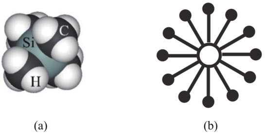
Figure 2: (a) Tetramethylsilane (TMS) molecule. (b) Schematic picture of the star-topology spin network of TMS. The open circle is System I (²⁹Si nucleus) while the filled circles form System II (H nuclei).

III.2 FID Signals

Figure 3 shows the theoretical and experimental FID’s. The right panels are the normalized experimental FID’s while the left panels show the theoretical ones. We plot the real (imaginary) parts of the normalised FID’s. In the right panels, we also show smooth curves obtained by moving-averaging the experimental data, which will be used to calculate non-Markovianity in the next subsection.

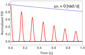
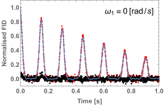
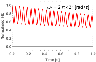
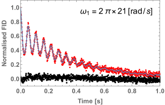
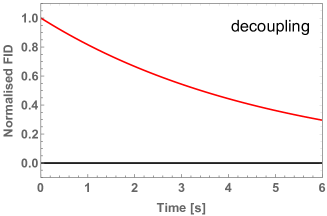
Figure 3: Left three panels show the theoretical results while the right ones show the corresponding experimental data. The red (black) lines represent the real (imaginary) parts of normalised FID’s. In theoretical dynamics, we employed the parameters $(\gamma_{\rm I},\gamma_{\rm II},J)=(0.41,0.20,2\pi\times 6.6)$ rad/s  [15]. $\omega_{1}$ is shown on the top right of each panel. The blue lines in the right panels are obtained by moving-averaging the corresponding experimental data. The dotted line in the top-left panel is $e^{-\gamma_{I}t/2}$, which shows the direct influence of the Markovian environment on System I.

Clearly, theoretical calculations well reproduce the experimental FID’s in both the Markovian (decoupling) and non-Markovian ($\omega_{1}=0$ rad/s) limits, as discussed in Ref. [15]. The peaks in the top-left panel are smaller than $e^{-\gamma_{\rm I}t/2}$ which implies that the information stored in System I can flow into the environment through System II. In other words, the information can escape into the environment even if $\gamma_{\rm I}=0$. In the intermediate region ($\omega_{1}=2\pi\times 21$ rad/s case in Fig. 3), we can see that our theoretical dynamics qualitatively agree with the experimental data. However, there is a quantitative difference between theory and experiment. The observed decay is faster than the theoretical prediction. This difference can be attributed to spatial inhomogeneity of $\omega_{1}$ [29]. The sample was sealed in an NMR test tube with finite size and $\omega_{1}$ is slightly different for TMS molecules at different parts of the tube. The observed FID signal is a result of ensemble average over a macroscopic number of TMS molecules from various positions in the test tube and they have dynamics corresponding to the local $\omega_{1}$. As a result, the observed FID signal involves average over $\omega_{1}$, namely average over different dynamics, which leads to faster decay. For the non-Markovian limit, such spatial inhomogeneity does not occur since $\omega_{1}=0$. The Markovian (decoupling) limit is now achieved by WALTZ-16, a decoupling pulse sequence robust against spatial inhomogeneity of $\omega_{1}$ [30]. This is the reason why theory well reproduces the experimental observation in both limits.

III.3 Engineering Non-Markovianity

Let us study how non-Markovianity measure $\cal N$ changes as a function of $\omega_{1}$ in our theory and experiment. We evaluate ${\cal N}$ from the analytical solution of $\beta_{12}(t)$ as shown in Fig. 4. The upper limit of the integration (48) is taken to be $t=50~{}{\rm s}\sim 20/\gamma_{\rm I}$ instead of $t\rightarrow\infty$, which is sufficiently large compared to the time scale $2/\gamma_{\rm I}$ of the dynamics.

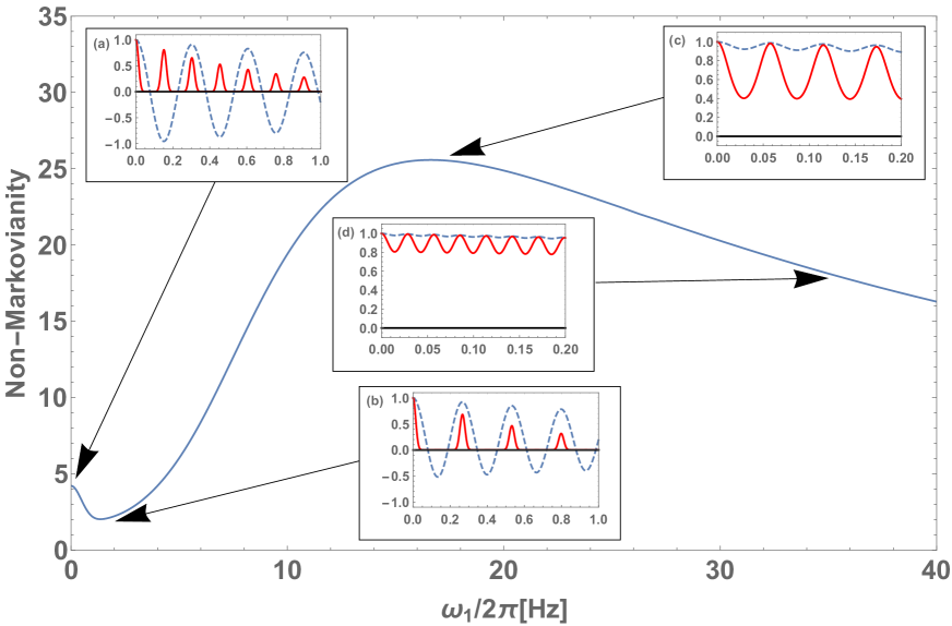
Figure 4: Non-Markovianity measure ${\cal N}$ as a function of $\omega_{1}$. Each inset shows the dynamics of the FID signal $\beta_{12}(t)$ (red line) and $\beta_{1}(t)$ (dashed blue line) for the corresponding $\omega_{1}$: (a) $\omega_{1}=0$ rad/s, (b) $\omega_{1}=2\pi\times 1.8$ rad/s, (c) $\omega_{1}=2\pi\times 17$ rad/s and (d) $\omega_{1}=2\pi\times 35$ rad/s. The plotted time interval of insets (a) and (b) is $[0,1.0]$ s while that of (c) and (d) is $[0,0.2]$ s. The parameters are $(\gamma_{\rm I},\gamma_{\rm II},J)=(0.41,0.20,2\pi\times 6.6)$ rad/s.

Note that $\cal N$ does not decrease monotonically in this theoretical curve. There is a dip in the small $\omega_{1}$ region. This behaviour is understood by examining insets in Fig. 4, which plots $\beta_{12}(t)$, the FID signal of the $(1+12)$-system. We also plot $\beta_{1}(t)$ for comparison. The magnitude of the signal is suppressed as a power of $n$ in the vicinity of $t$ satisfying $\beta_{1}(t)=0$ (Inset (a) in Fig. 4). The time intervals with such suppressed signals hardly contribute to ${\cal N}$. While $\omega_{1}$ increases, the oscillation centre of $\beta_{1}(t)$ is gradually lifted up. Suppression occurs prominently when the lower end of the oscillation is located around zero (Inset (b)); thus ${\cal N}$ first decreases near $\omega_{1}\sim 0$ and hits the minimum. After $\beta_{1}(t)$ is lifted up totally above zero, $n$ rather enhances the non-Markovianity since the oscillation is amplified according to the power of $n$ (Inset (c)). This causes the dip shown in Fig. 4. In the remaining region, ${\cal N}$ monotonically decreases since the oscillation gradually disappears (Inset (d)).

We show ${\cal N}$ obtained from the experimental data in Fig. 5. To avoid influence of the spatial inhomogeneity of $\omega_{1}$, we truncate the upper limit of the integration at a short time, $t=0.2$ s. In experiments, ${\cal N}$ is evaluated by using the moving-averaged experimental data explained in Fig. 3. We also give ${\cal N}$ for the theoretical dynamics with the same truncated integration interval to be compatible with the experimental results. The outline of this theoretical curve is the same as the curve shown in Fig. 4 although this curve has ripple structure because of the truncated integration interval. We see that the dip and peak in the experimental result are qualitatively reproduced by the theoretical calculation. The experimental results, however, basically shows smaller ${\cal N}$ than theoretical ones. This difference can be understood as the effect of the spatial inhomogeneity of $\omega_{1}$ as discussed in Sec. III.2. The faster decay of FID signals in the experiment makes ${\cal N}$ smaller.

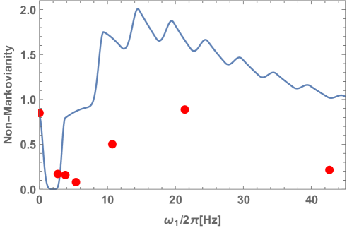
Figure 5: Non-Markovianity ${\cal N}$with a truncated integral interval $[0,0.2]$ s. The blue line is a theoretical result while the red points are obtained from the experimental data.

IV Summary

We have proposed an open-system model of which dynamics can be continuously tuned from non-Markovian to Markovian by changing an external field. The model consists of System I that is the principal system of interest, System II surrounding System I, and Markovian environment. We have shown that the dynamics of this model can be solved analytically with a reasonable initial condition. We compared our theoretical results with the experimental data.

We have shown that the results of the theoretical model qualitatively agree with the experimental results: in particular, the transition from Markovian to non-Markovian dynamics is well reproduced. Then we evaluated non-Markovianity of our model by introducing a non-Markovianity measure $\cal N$ based on the trace distance. Our model is expected to serve to understand non-Markovian open systems.

Appendix A Exact solution of Eq. (20)

Here we will show the exact form of $b_{0}(t)$ by solving Eq. (20). To do this, it is enough to find the eigenvalues and eigenvectors of ${\mathbb{M}}^{\prime}$ defined as

$${\mathbb{M}}^{\prime}:=2{\mathbb{M}}^{\rm T}=\begin{pmatrix}0&0&-iJ\\ 0&-\gamma_{\rm II}&-2\omega_{1}\\ -iJ&2\omega_{1}&-2\gamma_{\rm II}\end{pmatrix}.$$ (50)

The eigenvalues of ${\mathbb{M}}^{\prime}$ are

$$\lambda_{1}=-\gamma_{\rm II}-\frac{D}{C}+\frac{C}{3},\,\,\,\,\lambda_{2}=-\gamma_{\rm II}-\frac{D}{C}-\Bigl{(}\frac{1-\sqrt{3}i}{2}\Bigr{)}\frac{C}{3},\,\,\,\,\lambda_{3} =\lambda_{2}^{*}$$

$$C=\Bigl{(}54\gamma_{\rm II}\omega_{1}^{2}+3\sqrt{3}\sqrt{108\gamma_{\rm II}^{2}\omega_{1}^{4}+D^{3}}\Bigr{)}^{\frac{1}{3}},\,\,\,\,D=J^{2}-\gamma_{\rm II}^{2}+4\omega_{1}^{2}$$ (51)

Note that $C$ is always real with our parameters $(\gamma_{\rm I},\gamma_{\rm II},J)=(0.41,0.20,2\pi\times 6.6)$ rad/s. The corresponding (unnormalised) eigenvectors are given as

$$\vec{v}_{1}=\begin{pmatrix}1\\ -2i\frac{\omega_{1}}{J}\frac{\lambda_{1}}{\lambda_{1}+\gamma_{\rm II}}\\ i\frac{\lambda_{1}}{J}\end{pmatrix},\vec{v}_{2}=\begin{pmatrix}1\\ -2i\frac{\omega_{1}}{J}\frac{\lambda_{2}}{\lambda_{2}+\gamma_{\rm II}}\\ i\frac{\lambda_{2}}{J}\end{pmatrix},\vec{v}_{3}=\begin{pmatrix}1\\ -2i\frac{\omega_{1}}{J}\frac{\lambda^{*}_{2}}{\lambda^{*}_{2}+\gamma_{\rm II}}\\ i\frac{\lambda^{*}_{2}}{J}\end{pmatrix}.$$ (52)

By using the above eigenvalues and eigenvectors, the solution is written as

$$\begin{pmatrix}b_{0}\\ b_{y}\\ b_{z}\end{pmatrix}=\sum_{i=1,2,3}u_{i}\vec{v}_{i}\exp(\lambda_{i}t/2)$$ (53)

where $\{u_{i}\}_{i=1,2,3}$ are constant parameters determined by the initial condition. When assigning the initial values $(b_{0}(0),b_{y}(0),b_{z}(0))=(1,0,0)$, we obtain

$$u_{1} =\frac{|\lambda_{2}|^{2}(\lambda_{1}+\gamma_{\rm II})}{\gamma_{\rm II}\bigl{(}(\lambda_{1}-\lambda^{R}_{2})^{2}+(\lambda_{2}^{I})^{2}\bigr{)}},$$

$$u_{2} =\frac{\lambda^{2}_{1}\gamma_{\rm II}-\lambda_{1}(|\lambda_{2}|^{2}+2\lambda^{R}_{2}\gamma_{\rm II})}{2\gamma_{\rm II}\bigl{(}(\lambda_{1}-\lambda^{R}_{2})^{2}+(\lambda_{2}^{I})^{2}\bigr{)}}+i\frac{\lambda_{1}(\lambda_{1}-\lambda^{R}_{2})(|\lambda_{2}|^{2}+\lambda^{R}_{2}\gamma_{\rm II})+\lambda^{1}(\lambda^{I}_{2})^{2}\gamma_{\rm II}}{2\lambda^{I}_{2}\gamma_{\rm II}\bigl{(}(\lambda_{1}-\lambda^{R}_{2})^{2}+(\lambda_{2}^{I})^{2}\bigr{)}},$$

$$u_{3} =u_{2}^{*},$$ (54)

where we introduce the real (imaginary) part of $\lambda_{2}$: $\lambda_{2}=\lambda^{R}_{2}+i\lambda^{I}_{2},~{}\lambda^{R}_{2},\lambda^{I}_{2}\in{\mathbb{R}}$. Thus, the explicit form of $b_{0}(t)$ is

$$b_{0}(t) =u_{1}\exp(\lambda_{1}t/2)+u_{2}\exp(\lambda_{2}t/2)+u_{3}\exp(\lambda_{3}t/2)$$

$$=u_{1}\exp(\lambda_{1}t/2)+2\exp(\lambda^{R}_{2}t/2)\bigl{(}u^{R}_{2}\cos(\lambda^{I}_{2}t/2)-u^{I}_{2}\sin(\lambda^{I}_{2}t/2)\bigr{)},$$ (55)

where $u_{2}^{R}$ $(u_{2}^{I})$ is a real (imaginary) part of $u_{2}$. Note that $b_{0}(t)$ is always real with our parameters.

References

- [1] M.A. Nielsen and I.L. Chuang. Quantum Computation and Quantum Information. Cambridge Series on Information and the Natural Sciences. Cambridge University Press, 2000.
- [2] U. Weiss. Quantum Dissipative Systems. Series in Modern Condenced Matter Physics. World Scientific Publishing Company, 1999.
- [3] Vittorio Gorini, Maurizio Verri, and Alberto Frigerio. Non-markovian behavior in low-temperature damping: An application of the averaging method. Physica A: Statistical Mechanics and its Applications, 161(2):357 – 384, 1989.
- [4] Heinz-Peter Breuer, Elsi-Mari Laine, Jyrki Piilo, and Bassano Vacchini. Colloquium: Non-markovian dynamics in open quantum systems. Rev. Mod. Phys., 88:021002, Apr 2016.
- [5] Inés de Vega and Daniel Alonso. Dynamics of non-markovian open quantum systems. Rev. Mod. Phys., 89:015001, Jan 2017.
- [6] Jing Liu, Kewei Sun, Xiaoguang Wang, and Yang Zhao. Quantifying non-markovianity for a chromophore-qubit pair in a super-ohmic bath. Phys. Chem. Chem. Phys., 17:8087–8096, 2015.
- [7] Govinda Clos and Heinz-Peter Breuer. Quantification of memory effects in the spin-boson model. Phys. Rev. A, 86:012115, Jul 2012.
- [8] B. M. Garraway. Nonperturbative decay of an atomic system in a cavity. Phys. Rev. A, 55:2290–2303, Mar 1997.
- [9] D. Tamascelli, A. Smirne, S. F. Huelga, and M. B. Plenio. Nonperturbative treatment of non-markovian dynamics of open quantum systems. Phys. Rev. Lett., 120:030402, Jan 2018.
- [10] F. Ciccarello, G. M. Palma, and V. Giovannetti. Collision-model-based approach to non-markovian quantum dynamics. Phys. Rev. A, 87:040103, Apr 2013.
- [11] Andrea Chiuri, Chiara Greganti, Laura Mazzola, Mauro Paternostro, and Paolo Mataloni. Linear optics simulation of quantum non-markovian dynamics. Scientific Reports, 2:968 EP –, 12 2012.
- [12] Jiasen Jin, Vittorio Giovannetti, Rosario Fazio, Fabio Sciarrino, Paolo Mataloni, Andrea Crespi, and Roberto Osellame. All-optical non-markovian stroboscopic quantum simulator. Phys. Rev. A, 91:012122, Jan 2015.
- [13] J. F. Haase, P. J. Vetter, T. Unden, A. Smirne, J. Rosskopf, B. Naydenov, A. Stacey, F. Jelezko, M. B. Plenio, and S. F. Huelga. Controllable non-markovianity for a spin qubit in diamond. Phys. Rev. Lett., 121:060401, Aug 2018.
- [14] Ya-Nan Lu, Yu-Ran Zhang, Gang-Qin Liu, Franco Nori, Heng Fan, and Xin-Yu Pan. Observing information backflow from controllable non-markovian multichannels in diamond. Phys. Rev. Lett., 124:210502, May 2020.
- [15] Le Bin Ho, Yuichiro Matsuzaki, Masayuki Matsuzaki, and Yasushi Kondo. Realization of controllable open system with NMR. New Journal of Physics, 21(9):093008, sep 2019.
- [16] G. Lindblad. On the generators of quantum dynamical semigroups. Communications in Mathematical Physics, 48(2):119–130, Jun 1976.
- [17] V. Gorini, A. Kossakowski, and E.C.G. Sudarshan. Completely positive dynamical semigroups on -level systems. Journal of Mathematical Physics, 17:821–825, 1976.
- [18] M.H. Levitt. Spin Dynamics: Basics of Nuclear Magnetic Resonance. Wiley, 2008.
- [19] William B. Davis, Michael R. Wasielewski, Ronnie Kosloff, and Mark A. Ratner. Semigroup representations, site couplings, and relaxation in quantum systems. The Journal of Physical Chemistry A, 102(47):9360–9366, 1998.
- [20] Lorenza Viola. ”Experimental dynamical decoupling” in ”Quantum Error Correction”. Cambridge University Press, New York, 2013.
- [21] Frederico Brito and T Werlang. A knob for markovianity. New Journal of Physics, 17(7):072001, jul 2015.
- [22] Bassano Vacchini, Andrea Smirne, Elsi-Mari Laine, Jyrki Piilo, and Heinz-Peter Breuer. Markovianity and non-markovianity in quantum and classical systems. New Journal of Physics, 13(9):093004, sep 2011.
- [23] Sabrina Maniscalco and Francesco Petruccione. Non-markovian dynamics of a qubit. Phys. Rev. A, 73:012111, Jan 2006.
- [24] Yasushi Kondo, Mikio Nakahara, Shogo Tanimura, Sachiko Kitajima, Chikako Uchiyama, and Fumiaki Shibata. Generation and suppression of decoherence in artificial environment for qubit system. Journal of the Physical Society of Japan, 76(7):074002, 2007.
- [25] Heinz-Peter Breuer, Elsi-Mari Laine, and Jyrki Piilo. Measure for the degree of non-markovian behavior of quantum processes in open systems. Phys. Rev. Lett., 103:210401, Nov 2009.
- [26] Yasushi Kondo, Yuichiro Matsuzaki, Kei Matsushima, and Jefferson G Filgueiras. Using the quantum zeno effect for suppression of decoherence. New Journal of Physics, 18(1):013033, jan 2016.
- [27] Ai Iwakura, Yuichiro Matsuzaki, and Yasushi Kondo. Engineered noisy environment for studying decoherence. Phys. Rev. A, 96:032303, Sep 2017.
- [28] Yasushi Kondo and Masyuki Matsuzaki. Study of open systems with molecules in isotropic liquids. Modern Physics Letters B, 32(15):1830002, April 2018.
- [29] Elham Hosseini Lapasar, Koji Maruyama, Daniel Burgarth, Takeji Takui, Yasushi Kondo, and Mikio Nakahara. Estimation of coupling constants of a three-spin chain: a case study of hamiltonian tomography with nuclear magnetic resonance. New Journal of Physics, 14(1):013043, jan 2012.
- [30] T. D. W. Claridge. High-Resolution NMR Techniques in Organic Chemistry, volume 27 of TETRAHEDRON ORGANIC CHEMISTRY SERIES. Elsevier, second edition, 2009.