Magnetic Flux Ropes in the Solar Corona: Structure and Evolution toward Eruption ^∗

Abstract

Magnetic flux ropes are characterized by coherently twisted magnetic field lines, which are ubiquitous in magnetized plasmas. As the core structure of various eruptive phenomena in the solar atmosphere, flux ropes hold the key to understanding the physical mechanisms of solar eruptions, which impact the heliosphere and planetary atmospheres. Strongest disturbances in the Earth’s space environments are often associated with large-scale flux ropes from the Sun colliding with the Earth’s magnetosphere, leading to adverse, sometimes catastrophic, space-weather effects. However, it remains elusive as to how a flux rope forms and evolves toward eruption, and how it is structured and embedded in the ambient field. The present paper addresses these important questions by reviewing current understandings of coronal flux ropes from an observer’s perspective, with emphasis on their structures and nascent evolution toward solar eruptions, as achieved by combining observations of both remote sensing and in-situ detection with modeling and simulation. It highlights an initiation mechanism for coronal mass ejections (CMEs) in which plasmoids in current sheets coalesce into a ‘seed’ flux rope whose subsequent evolution into a CME is consistent with the standard model, thereby bridging the gap between microscale and macroscale dynamics.

1 Introduction

Large-scale ordered magnetic fields are ubiquitous in plasmas permeating the universe (Schrijver & Zwaan 2000; Beck 2012; Blackman 2015). Among them, helical magnetic fields have attracted great interest in diverse areas: they play important roles in fundamental physical processes such as magnetic reconnection and particle acceleration (e.g., Shibata & Tanuma 2001; Drake et al. 2006; Daughton et al. 2011); they are important agents in shaping the dynamics of the solar corona (e.g., Rust & Kumar 1996), of the heliosphere (e.g., Burlaga et al. 1981), and of the Earth’s magnetotail (e.g., Slavin et al. 2003), in coupling the interplanetary and planetary magnetic fields (e.g., Russell & Elphic 1979), and in propelling astrophysical jets with scales up to thousands of light years (e.g., Marscher et al. 2008). Additionally, according to the theory of plasma relaxation, a system with a fixed amount of magnetic helicity is destined to relax into a force-free, minimum-energy state of helical fields to the largest scale available (Taylor 1974, 1986; Blackman 2015).

Particularly, helical magnetic fields are observed to be systematically present in the solar atmosphere and to exhibit certain recurring patterns, e.g., the spiral shapes of sunspot fibrils (Hale 1927), helical-shaped filaments (e.g., Figure 1a; Rust & Kumar 1994; Pevtsov et al. 2003; Gilbert et al. 2007), sigmoidal-shaped coronal X-ray or EUV emissions (e.g., Figure 1b; Rust & Kumar 1996; Canfield et al. 1999; Sterling et al. 2000), and interplanetary magnetic clouds (MCs; Rust 1994). Interpretations of the sense of magnetic helicity in these observed structures have revealed a hemispheric helicity rule whereby patterns of negative helicity occur predominantly in the northern solar hemisphere, and those of positive helicity in the south (Pevtsov & Balasubramaniam 2003; Pevtsov et al. 2014).

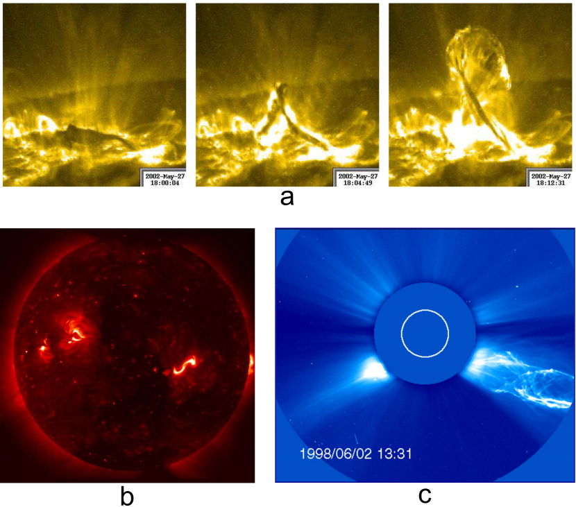
Figure 1: Exemplary helical structures observed in the solar atmosphere. a) Evolution of a filament observed at 195 Å by the Transition Region and Coronal Explorer (TRACE). The low-lying, dark filament first transforms into an inverted $\gamma$ and then an inverted $\delta$ shape through a rotation and writhing of the filament spine, which is a hallmark of the helical kink instability (Ji et al. 2003; Török & Kliem 2005; Gilbert et al. 2007). b) A full-Sun X-ray image from the X-Ray Telescope (XRT) on-board Hinode. A bright S-shaped structure is visible in the southwest quadrant. c) A coronal mass ejection (CME) observed by the Large Angle and Spectrometric Coronagraph (LASCO) on-board the Solar and Heliospheric Observatory (SOHO). A occulting disk obscures bright light from the photosphere and the white circle in the center indicates the size and location of the solar disk.

Often the term “magnetic flux rope” or “flux rope” is used to refer to a group of helical field lines collectively winding around a common axis. The proximity of the Sun makes the solar atmosphere an ideal laboratory to study the physics of flux ropes. A prodigious amount of data at multi-wavelengths, high cadence, and high resolution have been systematically collected for over the last fifty years. However, to explain the genesis of such an organized, coherent structure in the solar corona is a long-standing challenge, largely owing to the fact that we are still unable to properly measure the three-dimensional distribution of coronal magnetic fields. Further, in contrast to the coherency observed in coronal flux ropes, their footpoints ‘anchored’ in the dense photosphere are subject to turbulent shuffling motions due to the convection and granulation whose temporal and spatial scales are much smaller than those of coronal flux ropes (Stein 2012).

The size of coronal flux ropes spans quite a few orders of magnitude: flux ropes associated with coronal mass ejections (CMEs) are comparable in size as the Sun ($10^{7-8}$ km) and can retain their coherency when propagating through the Earth and beyond (Webb & Howard 2012); mini flux ropes in coronal jets may span only a few to tens of arcsecs ($10^{3-4}$ km; Patsourakos et al. 2008; Sterling et al. 2015); plasma blobs of scales $10^{4-5}$ km flowing intermittently along ray-like structures in the wake of CMEs (Lin et al. 2008) or above helmet streamers (Sheeley et al. 2009; Rouillard et al. 2010, 2011) are believed to be small flux ropes formed and ejected through magnetic reconnection in the rays. Similarly, interplanetary flux ropes have a diverse size distribution. Magnetic clouds (MCs) typically lasts one day (or about 0.1 AU) at the Earth’s orbit, as compared with much smaller flux ropes whose durations range from tens of minutes to a few hours (Cartwright & Moldwin 2008; Chen et al. 2019).

A flux rope’s magnetic twist implies that it possesses field-aligned electric currents inside the rope in the low-$\beta$ coronal environment. It has been debated whether coronal flux tubes are isolated and therefore current-neutralized (Melrose 1995; Parker 1996; Melrose 1996, 2017). In case of neutralization, the current flowing in the corona as expected from a twisted or sheared magnetic flux tube, also known as ‘direct current’, is completely canceled by a ‘return current’ that flows in the opposite direction around the tube, supposedly at its surface, which shields the ambient field from the direct current, therefore suppressing any current-driven instabilities. However, both observation (e.g., Georgoulis et al. 2012; Cheng & Ding 2016; Liu et al. 2017b) and numeric modeling (e.g., Török et al. 2014; Dalmasse et al. 2015) are against current neutralization. In case of non-neutralization, two mechanisms might be at work to produce the twisted fields: they can be twisted by photospheric and sub-photospheric flow motions (Klimchuk & Sturrock 1992; Török & Kliem 2003; Yan et al. 2015; Dalmasse et al. 2015), or transported into the corona through the emergence of current-carrying flux tubes (Leka et al. 1996; Longcope & Welsch 2000; Fan 2001; Török et al. 2014). With the measurements of photospheric transverse magnetic fields becoming more reliable, it has been revealed that electric currents tend to be non-neutralized in flare- and CME-producing active regions (Wheatland 2000; Georgoulis et al. 2012; Liu et al. 2017b; Kontogiannis et al. 2017), especially when magnetic shear is present around polarity inversion lines (PILs). Although the controversy has not been completely settled, many studies support that current-driven instabilities and current-channel interactions are important triggering mechanisms for solar eruptions.

In this review, we will first introduce how to identify flux ropes by quantifying magnetic connectivty and magnetic twist (§ 2), and recapitulate key observational and modeling results relevant to flux ropes in the solar corona, particularly in solar eruptions (§ 3). We then focus on what we have learned about how a flux rope forms and evolves toward eruption in the corona (§ 4), and how a flux rope is structured (§ 5), including its twist profile (§ 5.1) and boundary structure (§ 5.2), as well as more complex configurations such as ‘double-deckers’ (§ 5.3). We also draw the reader’s attention to other reviews devoted to magnetic flux ropes in the solar atmosphere as well as in interplanetary space, including, but not limited to, Russell et al. (1990); Marubashi (2000); Low (2001); Démoulin (2008); Linton & Moldwin (2009); Filippov et al. (2015); Cheng et al. (2017); Chen (2017); Gibson (2018); Wang & Liu (2019).

2 Quantification and Identification

2.1 Magnetic Topology

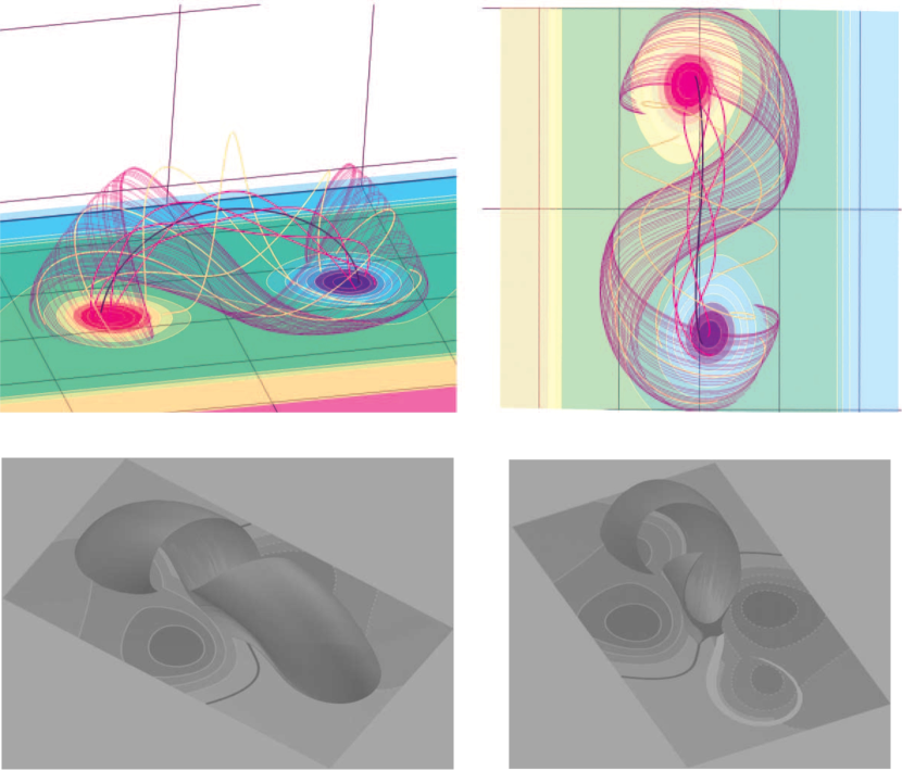
Figure 2: Topological structures associated with a flux rope embedded in a potential field. Top: a bald patch separatrix surface (BPSS) in different perspectives (from Gibson et al. 2004). The BPSS is made up of the field lines (magenta) tangent to the photophsere at the bald patch (BP) points, and wraps around other sample flux-rope field lines (red and yellow). Bottom: a hyperbolic flux tube (HFT; left) and the corresponding cross section in the center (right; from Titov 2007).

Despite their ubiquitous presence in plasmas, flux ropes have not been quantitatively defined. The term can loosely refer to any type of helical fields in the literature. Here we adopt a qualitative definition that is generally accepted by the solar community, i.e., a group of helical field lines collectively winding around a common axis. This simple description, however, has two important implications in regard to the coherence of the structure: 1) magnetic field lines inside the flux rope share similar orientations and are anchored in similar places at the photosphere, i.e., they have similar magnetic connectivities; 2) these fields lines hence have distinct magnetic connectivities than those surrounding the rope, i.e., a magnetic boundary may be present to separate the twisted field of a flux rope from its surrounding untwisted field.

Indeed, a flux rope whose underside is attached to the photosphere is wrapped around by a bald patch separatrix surface (BPSS; Titov & Démoulin 1999; Gibson & Fan 2006a, top panels in Figure 2). Separatrix surfaces define the boundaries of topologically distinct domains, and magnetic field lines threading a BPSS are tangent to the sections of the photospheric PIL called “bald patches”, where $(\mathbf{B}\cdot\nabla)B_{z}>0$ (Titov et al. 1993). On the other hand, a flux rope suspended in the corona is wrapped around by a hyperbolic flux tube (HFT; bottom panels in Figure 2), which is composed of two intersecting quasi-separatrix layers (QSLs), thin volumes across which field lines are drastically different in terms of magnetic connectivity. The HFT displays an X-shaped cross section beneath the flux rope (Titov 2007; Aulanier et al. 2010), hence is considered as the three-dimensional counterpart of the two-dimensional X-type magnetic null. When a BPSS flux rope rises in altitude, the BPSS configuration is transformed to HFT (e.g., Titov 2007; Aulanier et al. 2010). Both BPSS and HFT are the preferential sites for the formation of current-sheets, which can be driven by shearing motions of magnetic-field footpoints at the photosphere (e.g., Low 1987; Titov et al. 2003) or induced by MHD instabilities such as the helical kink instability (e.g., Fan & Gibson 2004; Török et al. 2004, see also § 3.2).

To understand the magnetic connectivities in an active region, one typically extrapolate the photospheric field into the higher solar atmosphere, because it is still impossible to measure the full three-dimensional distribution of the magnetic field from above the photosphere to the corona. Most extrapolations invoke the force-free assumption, which neglects non-magnetic forces in the low-$\beta$ corona, and consequently the Lorentz-force must also vanish in equilibrium. Compared with potential and linear force-free field extrapolations, the nonlinear force-free field (NLFFF) model is a more realistic approach by taking the force-free parameter $\alpha=\nabla\times\mathbf{B}/\mathbf{B}$ as a function of position. To understand the evolution of an active region, one may build a series of NLFFF models (e.g., Liu et al. 2016b). The force-free assumption may not be valid during the impulsive phase of the flares, when plasmas are accelerated primarily by Lorentz forces; but the flare-related changes of the coronal field can be inferred from a comparison of the NLFFF before and after the flare. For a self-consistent description of the plasma and magnetic field, however, one must relax the force-free assumption and turn to magnetohydrostatic or magnetohydrodynamic models (see the review by Inoue 2016; Wiegelmann et al. 2017).

Obviously, a flux rope may exist in any but the potential model of the coronal magnetic fields, but to identify and study the rope in a quantifiable manner, one must first quantify the magnetic connectivity and the magnetic twist, which are explicated below.

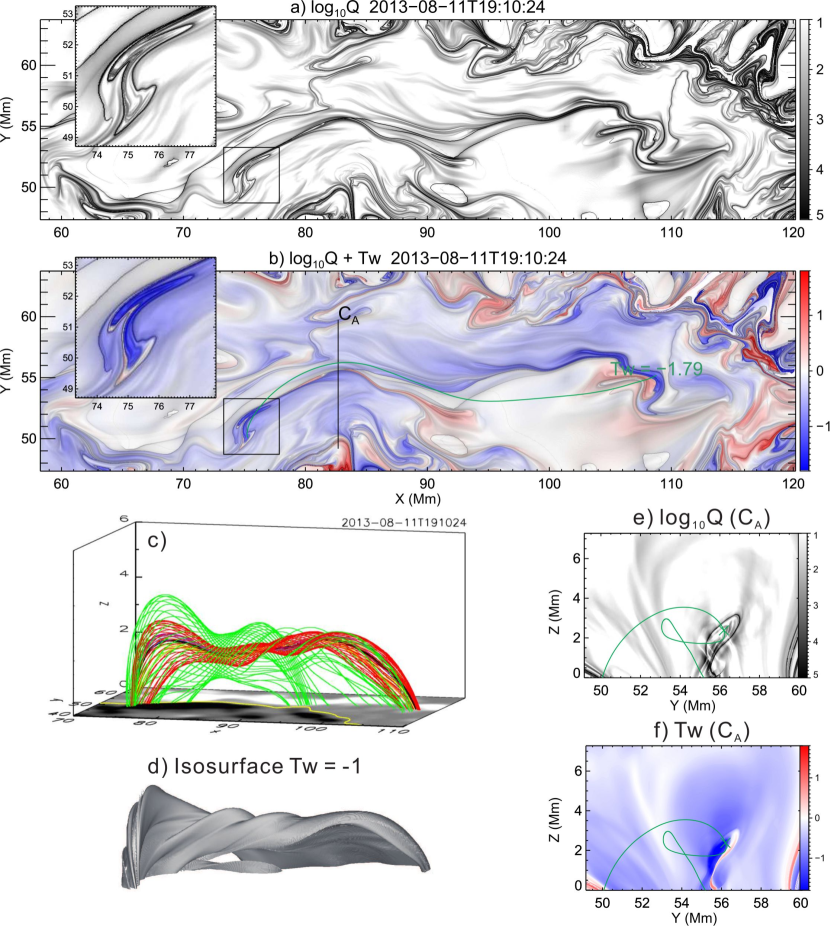
Figure 3: A flux rope identified in the NOAA active region 11817 before a C2.1-class flare on 2013 August 11 (adapted from Liu et al. 2016b). a) Distribution of $\log Q$ above 1 (white) and saturated at 5 (black) at the photosphere. b) Twist number saturated at $\pm 1.8$ and blended with the same distribution of $\log Q$ as in (a). In (a) and (b) a rectangle marks the flux rope’s eastern feet. This rectangular region is enlarged and redisplayed in the upper left corner. c) Three-dimensional perspective of the flux rope shown in field lines. Rainbow-colored field lines are in the vicinity of the axis (black). Red and green field lines are farther away from the axis. d) Isosurface of $T_{w}=-1$ viewed from the same perspective as (d). e) and f) show $\log Q$ and $T_{w}$ in a cutting plane C_A (marked in (b)), respectively. A representative twisted field line (dark green) of $T_{w}=-1.79$ is projected onto both C_A (e & f) and the photosphere (b). The symbol ‘x’ indicates where the field line threads the cutting plane.

2.2 Quantifying Magnetic Connectivity

Magnetic connectivities can be quantified by the squashing factor $Q$ of elemental magnetic flux tubes (Demoulin et al. 1996; Titov et al. 2002; Titov 2007), which is defined through the mapping between two footpoints of a field line that threads twice a plane, usually the photosphere, i.e., $\Pi_{12}:\mathbf{r}_{1}(x_{1},\ y_{1})\mapsto\mathbf{r}_{2}(x_{2},\ y_{2})$. With the Jacobian matrix of the mapping

$$D_{12}=\left[\frac{\partial\mathbf{r}_{2}}{\partial\mathbf{r}_{1}}\right]=\begin{pmatrix}\partial x_{2}/\partial x_{1}&\partial x_{2}/\partial y_{1}\\ \partial y_{2}/\partial x_{1}&\partial y_{2}/\partial y_{1}\end{pmatrix}\equiv\begin{pmatrix}a&b\\ c&d\end{pmatrix},$$ (1)

the squashing factor associated with the field line is given as follows

$$Q\equiv\frac{a^{2}+b^{2}+c^{2}+d^{2}}{|B_{n,1}(x_{1},y_{1})/B_{n,2}(x_{2},y_{2})|},$$ (2)

where $B_{n,1}(x_{1},y_{1})$ and $B_{n,2}(x_{2},y_{2})$ are the components normal to the plane of the footpoints, and their ratio is equivalent to the determinant of $D_{12}$. High-$Q$ structures (typically $Q\geq 100$), where the field-line mapping has a steep yet finite gradient, are referred to as quasi-separatrix layers (QSLs), whereas $Q\rightarrow\infty$ at topological structures (Titov et al. 2002). It is helpful to visualize these complex three-dimensional structures by calculating $Q$ in a three-dimensional volume box. This can be done by stacking up maps of $Q$ in uniformly spaced cutting planes (Liu et al. 2016b). To calculate such a $Q$-map in each cutting plane, the chain rule of the Jacobian is employed (Pariat & Démoulin 2012), e.g., if the above-mentioned field line threads a cutting plane at $\mathbf{r}_{c}(x_{c},y_{c})$, then

$$D_{12}=\left[\frac{\partial{\bf r}_{2}}{\partial{\bf r}_{1}}\right]=\left[\frac{\partial{\bf r}_{2}}{\partial{\bf r}_{c}}\right]\times\left[\frac{\partial{\bf r}_{c}}{\partial{\bf r}_{1}}\right],$$ (3)

where $[\partial\mathbf{r}_{c}/\partial\mathbf{r}_{1}]$ is given by its inverse,

$$\left[\frac{\partial{\bf r}_{c}}{\partial{\bf r}_{1}}\right]=\frac{1}{|B_{n,c}(x_{c},y_{c})/B_{n,1}(x_{1},y_{1})|}\begin{pmatrix}\partial y_{1}/\partial y_{c}&-\partial x_{1}/\partial y_{c}\\ -\partial y_{1}/\partial x_{c}&\partial x_{1}/\partial x_{c}\end{pmatrix},$$ (4)

so that each point on the cutting plane can be assigned a $Q$ value (see Tassev & Savcheva 2017 and Scott et al. 2017 for an alternative implementation). To eliminate spurious high-$Q$ structures introduced by field lines touching the cutting plane, i.e., $B_{n,c}(x_{c},y_{c})\rightarrow 0$, an optimal solution is to apply Eq. 3 to a local plane perpendicular to the field line under question (Titov 2007; Liu et al. 2016b).

2.3 Quantifying Magnetic Twist

Magnetic twist number measures how many turns a magnetic field line winds about the axis. For an idealized axisymmetric flux rope, this can be given by $B_{\phi}/rB_{z}$ in radians per unit length in cylindrical coordinates $(r,\phi,z)$, with $z$ along the rope axis. In practice, this approach cannot be directly applied to quantifying the intrinsic twist or ‘knottedness’ (Moffatt 1969) in flux ropes that do not possess a clearly defined axis. In general, suppose that $\mathbf{x}(s)$ is a smooth, non-self-intersecting curve parametrized by the arclength $s$, and that $\mathbf{y}$ a second such curve surrounding $\mathbf{x}$ to form a ribbon, Berger & Prior (2006, their Eq. 12) gave the number of turns that $\mathbf{y}$ makes about $\mathbf{x}$,

$$\mathcal{T}_{g}=\frac{1}{2\pi}\int_{\mathbf{x}(s)}\widehat{\mathbf{T}}(s)\cdot\widehat{\mathbf{V}}(s)\times\frac{d\widehat{\mathbf{V}}(s)}{ds}\,ds,$$ (5)

which is considered as the general definition of twist number; here $\widehat{\mathbf{T}}(s)=d\mathbf{x}/ds$ is the unit tangent vector to the axis curve, and $\widehat{\mathbf{V}}(s)$ is a unit vector normal to $\widehat{\mathbf{T}}(s)$ and pointing to $\mathbf{y}$ at the point $\mathbf{y}(s)=\mathbf{x}(s)+\varepsilon\widehat{\mathbf{V}}(s)$, so that $\mathbf{y}$ is also parameterized by $s$ along the axis curve $\mathbf{x}(s)$.

Berger & Prior (2006, their Eq. 16) gave an alternative twist number $\mathcal{T}_{w}$ to approximate $\mathcal{T}_{g}$ in the vicinity of $\mathbf{x}$ ($\varepsilon\ll 1$) in a magnetic field,

$$\mathcal{T}_{w}=\frac{\mu_{0}}{4\pi}\int_{L}\frac{\mathbf{J}\cdot\mathbf{B}}{B^{2}}\,dl.$$ (6)

In a force-free field, $\nabla\times\mathbf{B}=\alpha\mathbf{B}$, so that

$$\mathcal{T}_{w}=\frac{1}{4\pi}\int_{L}\alpha\,dl.$$ (7)

In particular, for a cylindrically symmetric flux tube of length $L_{z}$, it is well known that the twist number about the axis $z$ is

$$\mathcal{N}(r)=\frac{1}{2\pi}\frac{L_{z}B_{\phi}(r)}{rB_{z}(r)}.$$ (8)

Liu et al. (2016b) concluded that $\mathcal{T}_{g}$ is the generalization of $\mathcal{N}$, and $\mathcal{T}_{w}$ approaches $\mathcal{T}_{g}$ in the vicinity of the axis of a nearly cylindrically symmetric flux tube, but deviates otherwise. Below we derive succinctly the relations among these three twist numbers; readers are referred to Appendix C in Liu et al. (2016b) for details.

2.3.1 Relations among $\mathcal{T}_{g}$, $\mathcal{T}_{w}$, and $N$

To clarify the relationship between $\mathcal{T}_{g}$ (Eq. 5) and $\mathcal{T}_{w}$ (Eq. 6), we need express $d\widehat{\mathbf{V}}/ds$ in terms of physical quantities, in this case, the magnetic field. Obviously $\widehat{\mathbf{T}}(s)=\widehat{\mathbf{B}}(\mathbf{x}(s))=\mathbf{B}/B$ for magnetic field lines. The distance between $\mathbf{x}$ and $\mathbf{y}$ at point $s$, $\delta\mathbf{r}(s)=\varepsilon(s)\widehat{\mathbf{V}}(s)=\mathbf{y}(s)-\mathbf{x}(s)$, changes at a rate

$$\frac{d}{ds}\delta\mathbf{r}=\frac{d\mathbf{y}}{ds}-\frac{d\mathbf{x}}{ds}.$$

Given the arclength $s^{\prime}$ and unit tangent vector $\widehat{\mathbf{T}}^{\prime}$ at $\mathbf{y}$, we can rewrite $d\mathbf{y}/ds=d\mathbf{y}/ds^{\prime}\cdot ds^{\prime}/ds=\widehat{\mathbf{T}}^{\prime}\cdot ds^{\prime}/ds=\widehat{\mathbf{B}}(\mathbf{y}(s))\cdot ds^{\prime}/ds$. For $\varepsilon\ll 1$, $ds^{\prime}\approx ds$, so that

$$\frac{d}{ds}\delta\mathbf{r}\simeq\widehat{\mathbf{B}}(\mathbf{x}(s)+\delta\mathbf{r}(s))-\widehat{\mathbf{B}}(\mathbf{x}(s))\simeq\delta\mathbf{r}\cdot\frac{\partial\widehat{\mathbf{B}}}{\partial\mathbf{r}}.$$

Thus,

$$\frac{d\widehat{\mathbf{V}}}{ds}\simeq\widehat{\mathbf{V}}\cdot\frac{\partial\widehat{\mathbf{B}}}{\partial\mathbf{r}}-\frac{1}{\varepsilon}\frac{d\varepsilon}{ds}\widehat{\mathbf{V}}.$$ (9)

Inserting Eq. 9 into the local density of $\mathcal{T}_{g}$, we have

$$\frac{d\mathcal{T}_{g}}{ds}=\frac{1}{2\pi}\widehat{\mathbf{T}}\cdot\widehat{\mathbf{V}}\times\frac{d\widehat{\mathbf{V}}}{ds}\simeq\frac{1}{2\pi}\widehat{\mathbf{T}}\cdot\widehat{\mathbf{V}}\times\left(\widehat{\mathbf{V}}\cdot\frac{\partial\widehat{\mathbf{B}}}{\partial\mathbf{r}}\right).$$

Splitting $\partial\mathbf{B}/\partial\mathbf{r}$ into symmetric and antisymmetric parts, it can be derived that

$$\left[\widehat{\mathbf{V}}\cdot\frac{\partial\widehat{\mathbf{B}}}{\partial\mathbf{r}}\right]_{i}=\frac{1}{B}\left(\mathcal{S}_{ij}\widehat{V}_{j}+\frac{1}{2}\mu_{0}\epsilon_{jik}\widehat{V}_{j}J_{k}\right)-\frac{\widehat{T}_{i}}{B}\widehat{V}_{j}\frac{\partial B}{\partial x_{j}}.$$

Here $\mu_{0}\,\mathbf{J}=\nabla\times\mathbf{B}$ and $\mathcal{S}_{ij}\equiv[\mathbb{S}]_{ij}$ denotes the symmetric part of $\partial\mathbf{B}/\partial\mathbf{r}$. Generally, $\mathbb{S}\cdot\widehat{\mathbf{V}}=c_{1}\,\widehat{\mathbf{T}}+c_{2}\,\widehat{\mathbf{V}}+c_{3}\,\widehat{\mathbf{T}}\times\widehat{\mathbf{V}}$, where the coefficients $c_{1}$, $c_{2}$, and $c_{3}$ depend on both $\mathbb{S}$ and $\widehat{\mathbf{V}}$. With some vector calculus, it turns out that only the $c_{3}$ term of $\mathbb{S}\cdot\widehat{\mathbf{V}}$ and the antisymmetric part of $\partial\mathbf{B}/\partial\mathbf{r}$ remain:

$$\frac{d\mathcal{T}_{g}}{ds}\simeq\frac{c_{3}}{2\pi B}+\frac{\mu_{0}J_{\parallel}}{4\pi B},$$ (10)

where all quantities are taken at the axis field line $\mathbf{x}(s)$. In contrast, $\mathcal{T}_{w}$ (Eq. 6) is evaluated at the field line of interest, $\mathbf{y}(s)$. Thus,

$$\lim_{\varepsilon\to 0}\mathcal{T}_{w}(\varepsilon)=\mathcal{T}_{g}-\int_{\mathbf{x}(s)}\frac{c_{3}}{2\pi B}\,ds,$$ (11)

which specifies two conditions for $\mathcal{T}_{w}$ to reliably approximate $\mathcal{T}_{g}$: first, the field line must be sufficiently close to the axis such that $J_{\parallel}/B$ on $\mathbf{x}$ and $\mathbf{y}$ are approximately equal; second, the contribution from $\mathbb{S}$ proportional to $c_{3}$ can be negligible, in other words, the flux rope must possess certain degree of coherence. For example, in cylindrical symmetry, $B_{r}=0$, $B_{\phi}=B_{\phi}(r)$, and $B_{z}=B_{z}(r)$, all elements of $\mathbb{S}$ vanish identically except

$$S_{r\phi}\equiv\frac{1}{2}r\frac{\partial}{\partial r}\left(\frac{B_{\phi}}{r}\right),$$

which vanishes at the axis, too, for a smooth distribution of $J_{\parallel}(r)$. This is the case for both a constant-$\alpha$ force-free flux rope (Lundquist 1950) and a uniformly twisted flux rope(Gold & Hoyle 1960). Therefore the smaller the ratio of the two terms in Eq. 10, $2c_{3}/\mu_{0}J_{\parallel}$, locally the closer a flux rope approaches to cylindrical symmetry.

Now apply Eq. 5 directly to a cylindrical flux tube: for all $s$, $\widehat{\mathbf{T}}=\widehat{\mathbf{e}}_{z}$, $\widehat{\mathbf{V}}=\widehat{\mathbf{e}}_{r}$, and

$$\frac{d\widehat{\mathbf{V}}}{dz}=\frac{d\phi}{dz}\,\widehat{\mathbf{e}}_{\phi}.$$

From the field-line equation in cylindrical coordinates, $dr/B_{r}=rd\phi/B_{\phi}=dz/B_{z}=ds/B$, we recover the classical formula for $\mathcal{N}$ (Eq. 8),

$$\mathcal{T}_{g}=\frac{1}{2\pi}\int d\phi=\frac{1}{2\pi}\int\frac{B_{\phi}(r)}{rB_{z}(r)}dz=\mathcal{N}(r).$$

2.3.2 Application of $\mathcal{T}_{w}$

$\mathcal{T}_{g}$ is pertinent to strict stability analyses, but it depends on the precise determination of the axis, which is both non-trivial and demanding for numerical magnetic fields. On the other hand, $\mathcal{T}_{w}$ can be computed straightforwardly for any field lines. Approaching with caution, one can combine a map of $\mathcal{T}_{w}$ and the corresponding map of squashing factor $Q$ to conveniently identify and characterize flux ropes.

$\mathcal{T}_{w}$ is also useful in locating a flux rope’s axis, a necessary requirement for computing $\mathcal{T}_{g}$. One can see that from Eq. 6 the radial profile of $J_{\parallel}/B$, or $\alpha(r)$ in force-free fields, determines where $\mathcal{T}_{w}$ peaks in the cross section of flux ropes. For a flux rope with some degree of cylindrical symmetry, $\mathcal{T}_{w}$ reaches a local extremum at the axis, unless $J_{\parallel}/B$ is uniform around the axis. For example, $\mathcal{T}_{w}$ matches $\mathcal{N}$ at the axis in either a constant-$\alpha$ force-free flux rope (Lundquist 1950) or a uniformly twisted flux rope (Gold & Hoyle 1960); but away from the axis, $\mathcal{T}_{w}$ overestimates (underestimates) $\mathcal{N}$ in the former (latter) case (Appendix C in Liu et al. 2016b). This is further checked against an approximately force-free Titov-Démoulin flux-rope equilibrium (Titov & Démoulin 1999), using two different toroidal current density $J_{\mathrm{t}}(r)$, one roughly uniform, the other strongly peaked at $r=0$. $\mathcal{T}_{w}$ and $\mathcal{N}$ are found to agree to within 5% at the axis. $\mathcal{T}_{w}$ reaches the maximum (minimum) at the axis with the peaked (uniform) $J_{\mathrm{t}}(r)$ (Liu et al. 2016b).

Liu et al. (2016b) ran a tomography scan of a flux rope identified in the NLFFF by computing $\mathcal{T}_{w}$ maps in vertical cutting planes throughout the rope and tracing in each map a field line from the peak-$|\mathcal{T}_{w}|$ point. These field lines coincide within the limits of numerical accuracy over nearly the whole rope axis. This is further confirmed by cutting the rope perpendicularly at where it runs horizontally (e.g., at the apex point). The in-plane field vectors display a rotational pattern centered at the identified axis point, and that current density is enhanced normal to the cutting plane; both features are consistent with the existence of a flux rope (Liu et al. 2016b, their Figure 4). Outlined by high-$Q$ lines, the flux rope displays a rather compact and vertically elongated cross section (Figure 3(e & f)). Tracing field lines from points following this shape in the cutting plane (red lines in Figure 3c) or plotting the isosurface of $|\mathcal{T}_{w}|=1$ (Figure 3d) demonstrates the three dimensional configuration of this flux rope.

To summarize, one can define a coherent flux rope as a three-dimensional volume of enhanced $|\mathcal{T}_{w}|$ as enclosed by QSLs or BPSS. In the cross section of a flux rope with approximate cylindrical symmetry, the axis is located at the local extremum of the $|\mathcal{T}_{w}|$ map, unless $J_{\parallel}(r)/B(r)$ is uniformly distributed. This criteria has helped identify flux ropes of various configurations in various extrapolations (e.g., Wang et al. 2015a, 2017b; Yang et al. 2016; Liu et al. 2017a; Zhu et al. 2017; Awasthi et al. 2018; Su et al. 2018) or MHD models (e.g., Guo et al. 2017; Jiang et al. 2018) of coronal magnetic fields.

2.3.3 Field Line Helicity

An alternative quantity to characterize flux ropes is the field line helicity, which is given by an integral along a magnetic field line of length $L$

$$\mathcal{A}(L)=\int_{L}\frac{\mathbf{A}\cdot\mathbf{B}}{B}\,dl$$ (12)

where $l$ is the field-line arclength and $\mathbf{B}=\nabla\times\mathbf{A}$. However, the vector potential $\mathbf{A}$ is gauge-dependent and nonlocal, so is $\mathcal{A}$ (Yeates & Hornig 2016). Alternatively, $\mathcal{A}$ can be calculated as the limit in the infinitesimal tubular volume $D_{\epsilon}$ around the magnetic field line, which possesses magnetic flux $\Phi_{\epsilon}$ and an infinitesimal radius $\epsilon$ (Berger 1988),

$$\mathcal{A}(L)=\lim_{\varepsilon\to 0}\frac{1}{\Phi_{\epsilon}}\int_{D_{\epsilon}}\mathbf{A}\cdot\mathbf{B}\,dV.$$ (13)

Integrating over all field lines $L\supset D$ gives the total helicity $H=\int_{D}\mathbf{A}\cdot\mathbf{B}\,dV$ in the volume $D$. Thus, the field line helicity effectively describes how $H$ is distributed within the coronal volume, and flux ropes can be identified as concentrations of high field-line helicity in the corona (Yeates & Hornig 2016; Lowder & Yeates 2017). Naturally, $\mathcal{A}$ is correlated with $\mathcal{T}_{w}$ (Yeates & Hornig 2016). This is because the helicity within the infinitesimal tubular volume $D_{\epsilon}$ can be written as $H_{\epsilon}=\Phi_{\epsilon}\mathcal{A}\simeq\Phi_{\epsilon}^{2}\mathcal{T}_{w}$, if we neglect the contribution from the writhe assuming that the flux tube is not highly kinked, and if we consider only the self-helicity assuming that the field line is isolated. The same argument applies to calculating the helicity of a flux rope by its twist (Guo et al. 2013). With these assumptions, one has

$$\mathcal{A}\simeq\mathcal{T}_{w}\Phi_{\epsilon}.$$ (14)

However, since $\mathcal{A}$ is nonlocal, it remains an open question whether $\mathcal{A}$ can precisely quantify flux ropes, which often have a definite boundary.

3 Magnetic Flux Ropes in solar eruptions

Solar flares, filament/prominence eruptions, and coronal mass ejections (CMEs) in the solar atmosphere are the most spectacular phenomena in the solar system. Colloquially, when these events occur together, as they frequently do, we refer to them as solar storms. A typical storm releases more than $10^{32}$ ergs of energy, as it ejects up to $10^{16}$ g of plasma into interplanetary space with speeds often exceeding 1000 km s^-1, heats local coronal plasmas to temperatures in excess of 10 MK, and accelerates particles up to GeV energies.

Magnetic field plays a dominant role in solar storms, because in the solar atmosphere where most of the disturbances take place, the typical plasma $\beta$ is less than 0.1. It has been a consensus that solar eruptive phenomena draw energy from highly stressed magnetic fields in the corona (Forbes 2000). The magnetic field $\mathbf{B}$ can be always decomposed into a current-free, potential component $\mathbf{B}_{p}$ and a current-carrying, non-potential component $\mathbf{B}_{c}$, so that the magnetic energy $E_{m}$ in a volume $V$ can be written as (Sakurai 1981)

$$E_{m}=\int_{V}\frac{B^{2}}{8\pi}\,dV=\frac{1}{8\pi}\int_{V}B_{p}^{2}\,dV+\frac{1}{2c}\int_{V}\mathbf{A}_{c}\cdot\mathbf{J}\,dV,$$ (15)

where $\mathbf{B}_{c}=\nabla\times\mathbf{A}_{c}$ and $\mathbf{J}=\frac{c}{4\pi}\nabla\times\mathbf{B}_{c}$, because $\nabla\times\mathbf{B}_{p}=0$. In the solar atmosphere, the first term is the energy of the potential field produced by sub-surface currents, which is inaccessible to the coronal plasma. The free energy powering solar eruptions can only be contained in the second term carrying electric currents above the surface. Indeed, the gradual buildup of free energy over days or even weeks prior to eruptions in active regions is typically manifested as the development of strong-field, strong-gradient, highly-sheared polarity-inversion lines (PILs; Toriumi & Wang 2019). Obviously the field around such a PIL carries significant electrical currents because a current-free field is perpendicular to the PIL. It is debatable whether such electric currents represent the presence of a flux rope before eruption (see § 4.1).

3.1 Observation

From observational perspective, flux ropes are clearly present “after” CMEs, as evidenced, in particular, by in-situ detected magnetic clouds at 1 AU (Burlaga et al. 1981, see also Figure 9b), which possess a stronger, smoothly rotating magnetic field and a lower ion temperature than the ambient solar wind. Considerable efforts have been invested into developing flux rope models to characterize magnetic clouds, based on in-situ measurements of magnetic field and plasma parameters along the single-point traversing path made by spacecrafts through magnetic clouds. The approach varies from parametric fitting with different flux-rope solutions (e.g., Burlaga 1988; Wang et al. 2015b), including the famous linear force-free Lundquist solution (Lundquist 1950) with twist increasing from the axis to the boundary and the nonlinear force-free Gold-Hoyle solution with uniform twist (Gold & Hoyle 1960), to the Grad-Shafranov reconstruction based on the magnetohydrostatic theory (Hu & Sonnerup 2002; Hu 2017). The geometry of models ranges from symmetric cylinder (e.g., Burlaga 1988), asymmetric cylinder (e.g., Mulligan & Russell 2001) to torus (e.g., Marubashi & Lepping 2007). Cane & Richardson (2003) found that 100% of the interplanetary counterparts of CMEs (ICMEs) detected during solar minimum were magnetic clouds, but the fraction reduces to $<20$% during solar maximum. Some authors argue that all ICMEs contain a flux rope (e.g., Gopalswamy et al. 2013; Xie et al. 2013; Hu et al. 2014). Awasthi et al. (2018), on the other hand, found that a complex ICME originates from a system of multiple flux ropes braiding about each other.

Near the Sun, about 1/3 of CMEs exhibit a three-part structure of a bright loop front ahead of an emission-depleted cavity embedding a bright core, which is often attributed to prominence material (Illing & Hundhausen 1986). Recent observations, however, demonstrate that the CME core can also arise from the eruption of a flux rope void of prominence material (Howard et al. 2017; Veronig et al. 2018; Gou et al. 2019; Song et al. 2019). The three-part structure can often be traced back to a coronal streamer with a teardrop-shaped cavity underneath. It was recognized early that the cavity rather than the prominence core drove the CME (Hundhausen 1987). Generally, concave-upward or circular or helical features that appear before or during CMEs are believed to be consistent with the flux-rope geometry, and such CMEs are referred to as “flux rope CMEs” (Dere et al. 1999; Krall 2007; Vourlidas et al. 2013). Taking into account loop-CMEs that exhibit a bright loop font followed by emission depletion and jet-CMEs that contain helical structures, Vourlidas et al. (2013) estimated the occurrence rate of flux-rope CMEs to be 41%, which is close to the occurrence rate (35%) of magnetic clouds among ICMEs (Chi et al. 2016). In particular, a streamer may gradually swell into a slow CME with a three-part structure, leaving the streamer significantly depleted in its wake. Such “streamer blowout” CMEs exhibit the flux rope morphology at a much higher rate (61%) than regular CMEs (Vourlidas & Webb 2018).

Below we focus on filaments and sigmoids, which are of most frequently observed CME progenitors and of most trusted flux-rope indicators on the Sun. Many observational features of filaments and sigmoids can be naturally explained by a flux-rope model. A caveat to keep in mind is that most of these features, if not all, can also be accommodated by a sheared magnetic arcade consisting of weakly twisted field lines, which wind less than a full turn about a central axis.

3.1.1 Filaments

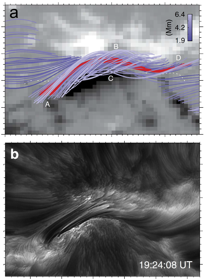
Figure 4: Extrapolated flux rope in relation to an active-region filament (from Wang et al. 2015a). a) Twisted field lines (red) surrounded by less twisted field lines (purple) from a NLFFF extrapolation model of the NOAA active region 11817 before a C2.1-class flare on 2013 August 11. The field lines are projected upon the photospheric $B_{z}$ distribution. b) The filament located within the same active region is observed with a spatial resolution as high as 60 km at the $H\alpha$ line center by the 1.6-m Goode Solar Telescope.

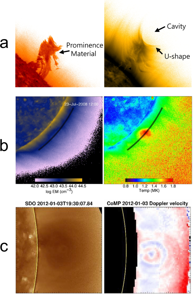
Figure 5: Structures of coronal cavities. a): A cavity observed by SDO/AIA at 304 Å (left) and at 171 Å (right; negative image) on 2010 June 13 (from Régnier et al. 2011). b): A cavity observed by Hinode/XRT on 2008 July 23 (from Reeves et al. 2012). The maps of emission measure (left) and temperature (right) are derived using the XRT Thin-Be/Ti-poly filter pair. c): A coronal cavity observed by SDO/AIA at 193 Å on 2012 January 3 (left) and the corresponding Doppler velocity pattern obtained by the Coronal Multi-Channel Polarimeter (CoMP) (right; from Bąk-Stȩślicka et al. 2013).

Solar filaments are composed of dense (10^11-12 cm^-3) and cold plasma (10⁴ K) suspended in the tenuous (10^8-9 cm^-3) and hot (10⁶ K) corona, hence appear dark in chromospheric lines such as H$\alpha$ against the solar disk, but in emission above the limb, hence termed prominences (see comprensive reviews by Tandberg-Hanssen 1995; Martin 1998; Mackay et al. 2010; Labrosse et al. 2010; Parenti 2014; Gibson 2018). Filaments are located in filament channels, where the chromospheric fibrils in H$\alpha$ are aligned with the PIL (Gaizauskas 1998). These fibrils are thought to give the direction of the magnetic field in the chromosphere. Similarly, filament threads are most likely aligned with magnetic field (Lin et al. 2005, see also Figure 4). In EUV, a dark corridor termed “EUV filament channel” is well extended in width beyond the H$\alpha$ filament. This is explained by Lyman continuum absorption of EUV radiation ($\lambda<912$ Å) and “volume blocking”, an additional reduction in EUV intensity because the cool plasma occupying the corridor does not emit any EUV radiation (Anzer & Heinzel 2005). Above the limb, the dense filament material is seen at the bottom of a cavity, which is density-depleted and overarched by coronal loops (Figure 5). These observations imply that the filament traces only a portion of a much larger, tunnel-like structure that extends from the photosphere throughout into the low corona.

Three distinct magnetic configurations have been proposed for filaments, namely the empirical wires (Martin & Echols 1994; Lin et al. 2008), the sheared magnetic arcade (Kippenhahn & Schlüter 1957), and the twisted flux rope (Kuperus & Raadu 1974). The empirical wire model assumes that a filament is composed of field-aligned fine threads. It differs from the other two in the absence of magnetic dips. Present either at the top of a sheared arcade or the bottom of a flux rope, magnetic dips are essential in supporting dense filament material against gravity, but become less indispensable when filament material is highly dynamic (Karpen et al. 2006). The flux-rope model is appealing in that its helical windings provide for filament material both the support against gravity and the thermal insulation from the hot corona. Besides, it demonstrates structural and morphological similarities with coronal cavities (§3.3 in Gibson 2018, see also Figure 5) as well as consistency with many active-region filaments (e.g., Dudík et al. 2008; Canou & Amari 2010; Sasso et al. 2014; Liu et al. 2014, 2016b, see also Figure 4). Further, it explains the inverse-polarity configuration observed often in quiescent filaments (Leroy et al. 1984; Bommier & Leroy 1998), i.e., the magnetic field traversing the filament is directed from negative to positive polarity. The sheared arcade model generally implies a normal-polarity configuration, which is more often found in active-region filaments than quiescent filaments. In reality, magnetic configurations of filaments can be complicated. For example, Guo et al. (2010b) found that a flux rope and a sheared arcade match two sections of a filament separately. A mixture of normal- and inverse-polarity dips is found in numerical experiments (Aulanier et al. 2002). To explain a ‘double-decker’ filament that was resolved stereoscopically and later erupted partially, Liu et al. (2012a) proposed two possible configurations, either a double flux rope or a single flux rope atop a sheared arcade. See §5.3 for more details.

The pattern of filament chirality provides an additional modeling constraint. By definition, a filament is dextral (sinistral) if its axial magnetic field points right (left) when a hypothetical observer is standing at the positive-polarity side of the PIL. It is believed that a dextral (sinistral) filament has right-bearing (left-bearing) barbs, a bundle of filament threads extruding out of the filament spine in a way similar to right- or left-bearing exit ramps off a highway. The majority of filaments in the northern (southern) hemisphere indeed have right-bearing (left-bearing) barbs and are overarched by left-skewed (right-skewed) coronal arcades, corresponding to the dominantly negative (positive) helicity in the same hemisphere (Martin 1998; Pevtsov et al. 2003; Yeates et al. 2007). However, it is argued that the correspondence between the filament chirality and the bearing sense of barbs works only for filaments supported by flux ropes and the correspondence is reversed for sheared arcades, if the sheared arcade possesses the same sign of helicity as the flux rope (Guo et al. 2010b; Chen et al. 2014). Alternatively, Chen et al. (2014) proposed that a filament is dextral (sinistral) if during the eruption the conjugate sites of plasma draining are right-skewed (left-skewed) with respect to the PIL. Employing this new criteria, it is found that the hemispheric rule of filament chirality is significantly strengthened (Ouyang et al. 2017; Zhou et al. 2020b).

In equilibrium, dense filament plasmas may only trace a portion of magnetic field lines, but when disturbed, they flow dominantly along field lines in a low-$\beta$ plasma environment, thereby providing clues on the magnetic configuration of the filament (e.g., Su & van Ballegooijen 2013; Awasthi et al. 2019; Awasthi & Liu 2019) or how it interacts with the surrounding field (e.g., Liu et al. 2018). It is also possible the observed flows represent motions of the magnetic structure itself instead of being along stationary field lines (Williams et al. 2009; Okamoto et al. 2016). It becomes even more elusive to determine the nature of mass motions in so-called tornado filaments (Li et al. 2012; Wang et al. 2017d). Counterstreaming flows along the filament spine (Schmieder et al. 1991; Zirker et al. 1998; Lin et al. 2003; Wang et al. 2018b) seem to be in favor of the sheared arcade model (e.g., Luna et al. 2012; Alexander et al. 2013; Zhou et al. 2020a); but within the cavity, swirling motions in plane of sky projection (Wang & Stenborg 2010; Li et al. 2012; Panesar et al. 2013; Wang et al. 2017d) and line-of-sight flows that forming a bullseye pattern (Bak-Steslicka et al. 2016, see also Figure 5c) are reminiscent of the nested toroidal flux surfaces of a flux rope’s cross section. Writhing deformations (e.g., Figure 1a; see also § 3.2.2) as well as unwinding motions (e.g., Yan et al. 2014; Xue et al. 2016) observed in erupting filaments also indicate the presence of magnetic twist.

Large-amplitude oscillations in filaments are also employed to probe the filament magnetic field. Often activated by shock waves impacting filaments side-on, transverse oscillations perpendicular to the filament spine are modeled by a damped harmonic oscillator with magnetic tension serving as the restoring force (Hyder 1966; Zhou et al. 2018). Longitudinal oscillations along the spine, on the other hand, are often activated by a subflare (e.g., Jing et al. 2003, 2006) or a jet (e.g., Luna et al. 2014; Awasthi et al. 2019) at one end of the filament, or, occasionally by a shock wave propagating along the filament spine (e.g., Shen et al. 2014). Various restoring forces have been considered since the discovery of this phenomenon (Jing et al. 2003), e.g., the magnetic pressure gradient (Vršnak et al. 2007), the gas pressure gradient (Jing et al. 2003; Vršnak et al. 2007), and the projected gravity in a magnetic dip (Jing et al. 2003; Zhang et al. 2012b; Luna & Karpen 2012). The first two forces have implications that are seldom observed, either predicting motions perpendicular to the local magnetic field (however, see Zhang et al. 2017) or requiring a temperature difference of several million Kelvins (Vršnak et al. 2007). The simple pendulum model, however, appears self-consistent and can provide magnetic parameters such as the curvature of the field-line dip and the minimum field strength (Luna & Karpen 2012; Luna et al. 2014; Zhou et al. 2017a, 2018). Awasthi et al. (2019) investigated mass motions driven by a surge initiated at one end of an active-region filament, and found that the filament material predominately exhibits rotation about the spine, which is evidenced by antisymmetric Doppler shifts about the spine, and longitudinal oscillations along the spine, featuring a dynamic barb extending away from the H$\alpha$ spine until the transversal edge of the EUV filament channel. Combined together, the composite motions are consistent with a double-decker structure comprising a flux rope atop a sheared-arcade system (see also § 5.3).

At the base of quiescent prominences, dome-like structures termed “bubbles” appear dark in H$\alpha$ and Ca II but bright in EUV (Berger et al. 2010). Sometimes they are observed to emerge from underneath and expand into quiescent prominences. The arc-shaped boundary of bubbles is an active location for the formation of rising ’plumes’ (Berger et al. 2010, 2011, 2017), which are suggested to be a probable source of mass supply into the prominence, as part of a “magneto-thermal convection” cycle to compensate the downward draining of prominence material (Berger et al. 2011). It is generally agreed that the bubble is filled with low-density plasma, which complicates the further plasma diagnostics, since most of the light we see may be coming from the foreground and background coronal plasma shining through the bubble. Gunár et al. (2014) argued that the apparent brightening is due to the prominence-corona-transition-region outside the bubble, which explains the presence of cool prominence material in the lines of sight intersecting the bubble. It is believed that the origin of prominence bubbles is associated with emergence of magnetic flux from below. Particularly, it is argued that bubbles could be formed due to perturbations in the prominence field by emerging parasitic bipoles from below (Dudík et al. 2012; Gunár et al. 2014). The absence of dips in the arcade field lines of the bipoles explains why a bubble is devoid of filament material (Dudík et al. 2012). Using He I D3 spectropolarimetric observations Levens et al. (2016) estimated that the magnetic field strength is higher inside the bubble than outside in the prominence. Thus, the rise of bubbles may be driven by the relatively large magnetic pressure rather than hot plasma inside the bubble. Naturally a magnetic separatrix or quasi-separatrix layer would form to separate the bubble from the surrounding prominence field, and the generation of plumes could be caused by reconnection at the separatrix (Dudík et al. 2012; Gunár et al. 2014; Shen et al. 2015), while the dynamic behaviors of plumes are consistent with the magnetic Rayleigh-Taylor and Kelvin-Helmholtz instabilities (Ryutova et al. 2010; Berger et al. 2017). The generation of large mushroom-headed plumes, a signature of the Kelvin-Helmholtz instability progressing into the non-linear explosive stage (Ryutova et al. 2010), seems conducive to the bubble formation and expansion (Awasthi & Liu 2019). Besides plumes, plasma inside bubbles can be dynamic. Awasthi & Liu (2019) observed a prominence bubble with a disparate morphology in the H$\alpha$ line-center compared to line-wings. Combining Doppler maps with flow maps in the plane of sky reveals a complex yet organized flow pattern inside the bubble, which is interpreted to be outlining a flux rope undergoing kink instability (see also § 3.2.2). Likely related to rising plumes, Zhang et al. (2014) found that prior to eruption a prominence is perturbed multiple times by underlying chromospheric fibrils that rise upward and merge into the prominence, whose subsequent eruption can be interpreted by a ‘flux feeding’ mechanism (see § 5.3).

3.1.2 Sigmoids

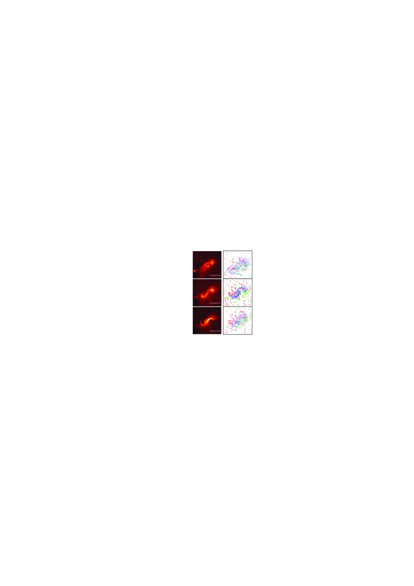
Figure 6: Evolution of a sigmoid (from Savcheva & van Ballegooijen 2009). Left: SXR images obtained by the X-Ray Telescope (XRT) on-board Hinode at different times, displaying a transformation from a double-J (top) to S (middle) configuration. When the sigmoid erupts (bottom), coronal dimmings can be seen inside the hooked parts of the S shape. Right:: selected field lines from NLFFF modeling with a flux-rope insertion method; in the background, red and green indicate positive and negative polarity, respectively.

Coronal sigmoids are S-shaped structures emitting in soft X-rays (SXR) and extreme ultraviolet (EUV) (Figure 6; Sakurai et al. 1992; Canfield et al. 1999; Moore et al. 2001). Typically the central part of a sigmoid is approximately aligned with the photospheric PIL, indicating the concentration of magnetic stresses and electric currents, hence they are described either by a flux rope (Rust & Kumar 1996; Titov & Démoulin 1999; McKenzie & Canfield 2008; Savcheva & van Ballegooijen 2009) or by a highly sheared magnetic arcade (Moore et al. 2001). Sigmoids are first discovered by the Soft X-Ray Telescope on-board Yohkoh, and soon recognized as an important CME progenitor (Canfield et al. 1999). In the wake of eruption, the sigmoid evolves into a post-flare cusp or arcade, known as the sigmoid-to-arcade evolution (Sterling et al. 2000). The majority of sigmoids are found to be forward (reverse) S-shaped in the southern (northern) hemisphere, following the hemispheric helicity rule, i.e., positive (negative) helicity is preferred in the southern (northern) hemisphere (Pevtsov et al. 2014).

Some sigmoids can be visible for days, but become bright only shortly prior to or during the early impulsive phase of flares. In a minority of SXR sigmoids, a continuous S shape is observed to appear through a transition from a double J shape prior to the onset of eruption (Figure 6). This transition is consistent with flux rope formation from a sheared arcade through reconnection (Green & Kliem 2009; Green et al. 2011; Green & Kliem 2014). Flux-rope models, however, suggest that the sigmoidal emission does not trace out the axis of the erupting flux rope, but highlight the formation of a sigmoidal current sheet at its underside (Titov & Démoulin 1999; Fan & Gibson 2003; Kliem et al. 2004; Savcheva & van Ballegooijen 2009, see also § 2.1).

More recently, the complexity in the structure and evolution of coronal sigmoids are further revealed by high-resolution SXR images obtained with the X-Ray Telescope on-board Hinode and high-resolution, high-cadence EUV images obtained with the the Atmospheric Imaging Assembly (AIA) onboard the Solar Dynamic Observatory (SDO). AIA is equipped with EUV filters sensitive to hot plasmas, such as the 94 Å (Fe 18, $\log T=6.85$) and 131 Å (Fe 21, $\log T=7.05$) passbands. Tripathi et al. (2009b) found that a double J-shaped hot arcs ($T>2$ MK) coexists with an S-shaped cold loop ($T\approx 1-1.3$ MK) bridging the gap of the double J structure in a decaying active region. This can be explained by the cooling of plasma carried by flux shells during earlier reconnection. Liu et al. (2010b) observed that an EUV sigmoid transforms continuously from a pair of opposing J-shaped loops first to a continuous S-shaped loop and then to a semi-circular eruptive structure (Figure 11(c1–c3)). The transformation in the latter stage, which is likely related to the rise of a faint, nearly linear feature in SXRs (Moore et al. 2001; McKenzie & Canfield 2008; Green et al. 2011) and is also recognized as the appearance of a “hot channel” in EUV (Zhang et al. 2012a), indicates the formation of a highly coherent but unstable structure, most likely a flux rope. The hot channel may appear different from different viewing angles, e.g., a blob if viewed along the axis (Cheng et al. 2011b; Nindos et al. 2015). Hundreds of hot channels have been detected by SDO/AIA in recent years (Zhang et al. 2015; Nindos et al. 2015), and detailed investigations into a few cases show that the hot channel forms either prior to the eruption onset, during a flare precursor or a slow-rise phase leading up to eruption (Liu et al. 2010b; Zhang et al. 2012a; Cheng et al. 2013a, b; Joshi et al. 2017), or during confined flares preceding the eruptive flare (Patsourakos et al. 2013).

3.1.3 Filament-Sigmoid Relationship

It is difficult to understand the relationship between filaments and sigmoids that are aligned along the same PIL. To be consistent with the hemispheric helicity rule, it is suggested that a sigmoid is represented by sigmoidal field lines threading the current sheet formed at the BPSS or HFT underneath an upwardly kinked flux rope, whose sense of S shape is opposite to that of the sigmoid (Titov & Démoulin 1999; Fan & Gibson 2003; Kliem et al. 2004; Savcheva & van Ballegooijen 2009). This scenario may find support in observations of the apex rotation during filament eruptions. Associated with a forward (reverse) S-shaped sigmoid, the filament apex rotates clockwise (counterclockwise) if viewed from above, suggesting that the filament is embedded in a right-handed (left-handed) flux rope (Green et al. 2007; Zhou et al. 2020b). However, it is unclear whether the flux rope already takes on an S shape opposite to the sigmoid before the eruption, because the cold filament and the hot sigmoid almost always display similar S shapes (e.g., Pevtsov 2002; Cheng et al. 2014b; Zhou et al. 2017b, 2020b). The filament can indeed reverse the sense of its S shape through apex rotations during the eruption (Rust & LaBonte 2005; Romano et al. 2005; Green et al. 2007; Zhou et al. 2020b). This may indicate that the sign of magnetic writhe is maintained when the originally low-lying flux rope rises to high altitudes during the eruption (Török et al. 2010).

However, this does not explain why the filament often survives the eruption, showing no significant changes beneath the post-flare arcade, which replaces the sigmoid during the eruption. In some cases one can clearly see the undisturbed filament underneath the sigmoid and between the two flare ribbons during the whole process of the eruption (Pevtsov 2002; Liu et al. 2007a; Cheng et al. 2014b), which excludes the possibility that a filament may reform immediately after the eruption. One possibility is that magnetic reconnection occurs within the flux rope but above the embedded filament, which leads to a CME without a corresponding filament eruption (Gilbert et al. 2000; Gibson & Fan 2006b; Liu et al. 2007b).

It is also possible that the low-lying filament and the high-lying sigmoid is only part of a much more complex structure, e.g., a double-decker (see § 5.3). Régnier et al. (2002) and Régnier & Amari (2004) employed NLFFF extrapolations to investigate the magnetic configuration of an S-shaped filament (height 30 Mm) and a sigmoid (height 45 Mm) aligned along the same PIL in the NOAA active region 8151. They found both structures have the similar S shape and can be described by a twisted flux tube with a twist number short of unity, but the electric current density is positive in the right-handed filament and negative in the left-handed sigmoid. In addition, a right-handed flux rope with a twist number slightly exceeding unity is present at a higher altitude (60 Mm). Thus, the structure is essentially consistent with one of the two double-decker configurations, comprising a flux rope atop a sheared arcade (see § 5.3; Liu et al. 2012a). Cheng et al. (2014b) invoked the other double-decker configuration, i.e., a double flux rope, to explain the sigmoid eruption on 2012 July 12: a low-lying flux rope associated the sigmoid and a co-spatial filament forms in two groups of sheared arcades a half day before the eruption; a high-lying flux rope in the form of an S-shaped hot channel appears 2 hrs before the eruption. Although only the low-lying rope is identified in the NLFFF model, the hot channel is verified to be a flux rope when it is detected in situ as a magnetic cloud three days later.

In partial eruptions, the filament-sigmoid association becomes more complicated. That a sigmoid splits during eruption or a sigmoid immediately reforms after eruption is often considered to be the signature of a BPSS flux rope whose lower part of the rope is tied to the dense photosphere (Gibson & Fan 2006b; Green et al. 2011). For a sigmoid forming in the underside of an HFT flux rope, it is expected that the whole flux rope is ejected and that the sigmoid ceases to exist after the eruption (Aulanier et al. 2010; Fan 2010, 2012). When a filament is involved, however, multiple factors may affect whether a full, partial, or failed filament eruption will occur; these include how much the magnetic dips are filled with filament material and where these material is located relative to where the rope breaks into two due to internal magnetic reconnections (Gibson & Fan 2006b; Gilbert et al. 2000, 2007). The brightening within a filament body and its subsequent splitting during eruptions is perhaps the most convincing observational signature of internal reconnections (Liu et al. 2008; Tripathi et al. 2009a; Cheng et al. 2018a), which may take place at a central vertical current sheet that forms as the rope writhes and expands upward, specifically, between the BPSS field lines and the ambient field lines, including those in the flux rope and the surrounding magnetic arcades (Gibson & Fan 2006a). Liu et al. (2008) reported that a discontinuous sigmoid becomes a continuous S lying above the filament at the eruption onset, yet both the filament and sigmoid still bifurcate during the eruption, suggesting that reconnections take place both above and within the filament. Alternatively, internal reconnections may naturally occur at the HFT within a double-decker configuration (see § 5.3) or between braided flux ropes (e.g., Awasthi et al. 2018).

3.2 Modeling

The eruptions in the solar atmosphere exhibit distinctly diverse patterns across a vast range of spatio-temporal scales, from CMEs in the shape of stellar-sized bubbles, to localized flares within active regions that harbor sunspots, to collimated jets down to the resolution limit of modern telescopes. Although the complexity and diversity of eruptive phenomena makes it impossible to build a ‘universal’ model that is capable of explaining all observational aspects in all events, the standard or CSHKP flare model (Carmichael 1964; Sturrock 1966; Hirayama 1974; Kopp & Pneuman 1976) is successful in explaining the major characteristics of two-ribbon eruptive flares, which provides a solid basis to understand the flare-CME coupling (see reviews by Forbes 2000; Priest & Forbes 2002; Forbes et al. 2006): destabilized by an unspecified trigger, a flux rope starts to rise and stretch the overlying magnetic field, also termed “strapping field”, which serves to constrain the rope; as a result, a vertical current sheet develops in the wake of the rope, where successive magnetic reconnections add layers of plasma and magnetic flux to the rope and simultaneously produce the growing flare loop system whose footpoints correspond to the separating flare ribbons in the lower atmosphere. By converting magnetic fluxes of the strapping field to those of the flux rope, the role of flare reconnection is therefore twofold: it reduces the downward-pointing but increases the upward-pointing Lorentz forces exerted upon the flux rope, making it rise and expand faster, which in turn enhances the plasma inflow toward the current sheet and therefore the reconnection rate. This positive feedback creates a snowballing CME propagating into the outer corona.

More recently, aided by nonlinear force-free field or MHD modeling of the coronal magnetic field, it has been demonstrated that H$\alpha$ and UV flare ribbons often coincide with the footprints of QSLs (e.g., Demoulin et al. 1997; Démoulin 2006; Liu et al. 2014, 2016a, 2018; Su et al. 2018; Jiang et al. 2018; Janvier et al. 2014, 2016). In particular, the footprints of QSLs wrapping around the flux rope correspond to a pair of J-shaped ribbons of high electric current densities, with their hooks surrounding the rope legs (Janvier et al. 2014, 2016; Wang et al. 2017c). In a data-driven MHD simulation, Jiang et al. (2018) tracked the footpoints of field lines newly reconnected at the HFT below the flux rope, where the QSL intersects itself. They found that the location of these footpoints not only match the observed flare ribbons as well as the boundary of the rope’s feet at far ends of the ribbons, but their evolution also emulates the temporal separation of the flare ribbons. Motivated by these observational and modeling results, it has been proposed that the two-dimensional standard model can be extended to three dimensions to address the shape, location, and dynamics of flares with a double J-shaped ribbons (Aulanier et al. 2013, 2012; Janvier et al. 2013, 2015).

The mainstream models of solar eruptions are in the ‘storage and release’ category, i.e. the free magnetic energy is quasi-statically accumulated in the corona on time-scales of days to weeks, and then rapidly released during the eruption on time-scales of minutes to hours (see the reviews by Chen 2011; Forbes et al. 2006; Forbes 2010). The key parameters and detailed processes that govern the evolution leading up to an eruption are not fully understood, nor does the pre-eruption magnetic configuration. But in all storage-and-release models, the core erupting structure is a flux rope, no matter it is embedded in the pre-eruption configuration or formed by magnetic reconnection on the fly. In the former scenario, including the standard flare model (Kopp & Pneuman 1976), the pre-existent flux rope may originally emerge from below the photosphere into the corona (e.g., Fan 2001; Roussev et al. 2012; Török et al. 2014), or form in the low corona by slow magnetic reconnection in a sheared magnetic arcade (van Ballegooijen & Martens 1989), which is driven by the gradual evolution of the magnetic field in the photospheric boundary (e.g., Amari et al. 2014). In the latter scenario, the initial state typically contains sheared arcades and a new flux rope forms via magnetic reconnection during the course of the eruption (Antiochos et al. 1999; Moore et al. 2001; Karpen et al. 2012).

The models of solar eruptions can also be categorized as either ideal or resistive according to the initiation and driving mechanism. In resistive models, magnetic reconnection is responsible for the onset and growth of the eruptive structure in time, as well as for the formation of the flux rope during the eruption (e.g., Antiochos et al. 1999; Moore et al. 2001). In ideal models, the coronal magnetic field reaches a critical point where a loss of equilibrium (also known as a ‘catastrophe’; e.g., Lin & Forbes 2000) or a loss of stability (e.g., Török & Kliem 2005; Kliem & Török 2006) occurs, leading to the eruption. Both catastrophe and instability can lead to the formation of a vertical current sheet underneath the flux rope, as in the standard flare model, but magnetic reconnection at the current sheet is only invoked as a byproduct in these ideal models. The two most frequently cited ideal MHD instabilities are the torus and the kink instability, both are driven by electric currents. It is argued that the catastrophe and the torus instability are equivalent descriptions for the eruption onset condition of a flux rope (Démoulin & Aulanier 2010; Kliem et al. 2014a). Below we first focus on the torus instability (§ 3.2.1) and the kink instability (§ 3.2.2), both involving a single flux rope, and then touch on instabilities involving interacting flux ropes or current systems (§ 3.2.3).

3.2.1 Torus Instability

The torus instability arises in a competition between the upward ‘hoop’ force, which is the Lorentz force between a toroidal current and its own poloidal field, and the downward ‘strapping’ force, which is the Lorentz force between the same toroidal current and an external potential field perpendicular to the axis of the torus (Bateman 1978; Chen 1989; Kliem & Török 2006). The torus instability, also termed lateral kink instability, sets in against expansion if the external field decreases fast enough in the direction of the major axis of the torus. The rate at which the field decreases with height is quantified by the decay index $n=-d\ln B/d\ln h$, where $h$ is the height above the photosphere. The threshold value of the instability $n_{\mathrm{crit}}$ is derived to be 1.5 for a toroidal current channel (Kliem & Török 2006), while for a straight current channel, $n_{\mathrm{crit}}\gtrsim 1$ (Démoulin & Aulanier 2010).

In comparison with the prototypical magnetic configuration of a CME progenitor, i.e., a flux rope is embedded in a sheared external field, which becomes less sheared at higher altitudes, approaching a potential field, one can see that both the toroidal component of the external field and the poloidal current of the flux rope are missing in the idealized, analytical models. Hence, it is not surprising that in numerical studies (e.g., Fan & Gibson 2007; Kliem et al. 2013; Zuccarello et al. 2015), $n_{\mathrm{crit}}$ is found to vary in a relatively wide range [1.4–2.0]. Additionally, the analysis in Kliem & Török (2006) applies to a slender flux rope. When it comes to a flux rope of finite size, it is unclear whether the decay index should be computed at the rope apex or axis (Zuccarello et al. 2016). In calculating the decay index, it is difficult to decouple the external magnetic field from the field induced by the electric currents inside the flux rope. The usual practice is to use the potential field extrapolated from the vertical component of the photospheric magnetic field to approximate the strapping field. This is because potential fields are expected to be perpendicular to PILs along which filament channels that host flux ropes are formed. But it is unclear as to how good the approximation is, especially when PILs are curved, and what role is played by the sheared, nonpotential component of the external field. Also, one may need take into account nonradial expansion that is frequently observed in filament eruptions (Liu et al. 2009b); one solution is to compute the decay index along the eruption direction (Duan et al. 2019).

In a laboratory experiment, Myers et al. (2015) recognized four separated regimes in the parameter space spanned by the torus instability parameter, decay index $n$, and the kink instability parameter, safety factor $q$, which is approximately the inverse of twist number (see §2.3). Besides the expected ‘stable’, ‘eruptive’, and ‘failed kink’ states, they found a new ‘failed torus’ regime, in which a torus-unstable but kink-stable flux rope fails to erupt, due to the Lorentz force between the rope’s poloidal current and the external toroidal field. When similar scatter plots are made for solar eruptions, it is unclear whether a failed torus regime actually exists (Jing et al. 2018; Zhou et al. 2019; Duan et al. 2019). Zhou et al. (2019) found that significant rotational motion, which may be caused by the helical kink instability, tends to be associated with failed filament eruptions that are normally judged to be torus unstable. However, the rotation driven by the helical kink instability cannot be easily distinguished from that caused by a Lorentz force resulting from the misalignment between the flux rope’s toroidal current and the external toroidal field (Isenberg & Forbes 2007; Kliem et al. 2012). Thus, it remains obscure as to what parameters can differentiate failed from successful CMEs.

Despite the simplifications and obscurities, how the magnetic field overlying an eruptive structure decays with height is indeed found to play an important role in regulating eruptive behaviors (e.g., Török & Kliem 2005; Liu 2008; Guo et al. 2010a; Cheng et al. 2011a; Zuccarello et al. 2014; Wang et al. 2017a; Baumgartner et al. 2018; Amari et al. 2018). Two types of $n(h)$ profiles emerge in observation (Guo et al. 2010a; Cheng et al. 2011a; Wang et al. 2017a): 1) $n$ increases monotonically as the height increases; and 2) the $n(h)$ profile is saddle-like, exhibiting a local minimum $n_{b}$ at a height higher than the critical height $h_{\mathrm{crit}}$ corresponding to $n_{\mathrm{crit}}=1.5$, which is approximately half of the distance between the centroids of opposite polarities in active regions (Wang et al. 2017a). The saddle-like $n(h)$ profile is found exclusively in active regions of multipolar field configuration, despite that the majority cases of monotonously growing $n(h)$ also originate from multipolar field. Supposedly the saddle-like profile provides a potential to confine an eruptive structure if the local minimum $n_{b}$ at the bottom of the saddle is significantly below $n_{\mathrm{crit}}$. Indeed Wang et al. (2017a) found that $h_{\mathrm{crit}}$ is significantly higher for confined flares than for eruptive ones, and that $n_{b}$ is significantly smaller in confined flares than that in eruptive ones. In a data-driven MHD simulation, Guo et al. (2019a) computed the decay index along the eruption path of a flux rope, and found that the rope starts to rise rapidly at the same height as the decay index crosses the canonical critical value of 1.5. Similarly, recent studies on the height-time profiles of eruptive filaments (Vasantharaju et al. 2019; Zou et al. 2019b; Myshyakov & Tsvetkov 2020; Cheng et al. 2020) and of hot channels (Cheng et al. 2020) generally concluded that the decay index at the height where the slow rise transitions to fast rise is close to the threshold of the torus instability.

The torus instability can be triggered or suppressed by magnetic reconnection that modifies the overlying field. This effect is often invoked to explain sympathetic eruptions, a sequence of eruptions that occur at different places within a relatively short time interval. The distanced regions can be connected by magnetic reconnection of large-scale magnetic field, as suggested by observational investigations (Liu et al. 2009a; Zuccarello et al. 2009; Schrijver & Title 2011; Schrijver et al. 2013; Jiang et al. 2011; Titov et al. 2012; Shen et al. 2012b; Yang et al. 2012; Joshi et al. 2016; Wang et al. 2016a, 2018a; Zou et al. 2019a) and corroborated by numerical simulations (Ding et al. 2006; Török et al. 2011; Lynch & Edmondson 2013). Unlike flare reconnection in active regions, Wang et al. (2018a) found that magnetic reconnection of the large-scale field in the quiet-Sun corona is subtly manifested through serpentine flare ribbons extending along chromospheric network, coronal dimmings, apparently growing hot loops, and contracting cold loops. The reconnection continually strengthens the strapping field of one filament that undergoes a failed eruption, but weakens the strapping field of the other that later erupts successfully.

3.2.2 Kink Instability

In a cylindrical flux rope of radius $a$ and length $L$, the safety factor $q(r)=rB_{z}(r)/LB_{\theta}(r)$, which is related to the twist angle through $\Phi=2\pi/q$, is key to the flux-rope stability. The external kink instability occurs when $q(a)<1$, which exceeds the Kruskal-Shafranov limit of one field-line turn about the flux-rope axis (Kruskal & Tuck 1958; Shafranov 1958). The kink is associated with the $m=1$ mode in the Fourier decomposition of linear perturbations in terms of $\exp(im\theta+ikz)$. This mode helically displaces the central axis as well as the surroundings, hence is also termed the helical kink instability. Taking into account the stabilizing effect of line-tying — both footpoints of any coronal flux tubes anchor firmly in the dense photosphere — Hood & Priest (1981) showed analytically that the critical value of twist angles for a force-free, uniform-twist equilibrium of infinite radial extent is $\Phi=2.49\pi$. The actual critical twist value turns out to be rather sensitive to equilibrium details (e.g., Einaudi & van Hoven 1983; Baty & Heyvaerts 1996; Baty 2001; Török & Kliem 2003), including the embedding of the flux rope in the external field, the radial twist profile, the radius of the rope, e.g., the critical twist number is larger for a thinner flux rope (see also Wang et al. 2016b), as well as the weight of prominence material at the bottom of the flux rope (Fan 2018).

The external kink instability has been proposed as a trigger for magnetic reconnection responsible for coronal heating (Browning et al. 2008; Hood et al. 2009) or flare heating (Hood & Priest 1979; Pariat et al. 2009; Srivastava et al. 2010). The invoke of this instability in solar eruptions is mainly motivated by the dramatic development of helical eruptive structures (e.g., Ji et al. 2003; Romano et al. 2003; Rust & LaBonte 2005; Williams et al. 2005; Alexander et al. 2006; Liu et al. 2007b; Patsourakos et al. 2008; Liu & Alexander 2009; Cho et al. 2009; Karlický & Kliem 2010; Kumar et al. 2012; Yang et al. 2012; Kumar & Cho 2014), typically when a filament rises and rotates into an inverted $\gamma$ or $\delta$ shape in projection (Figure 1a; Gilbert et al. 2007). These events exhibit not only a winding of the filament threads about the axis (e.g., Wang et al. 2015a, see also Figure 4b), arguing for the existence of considerable twist, but also an overall helical shape, indicating a writhed axis. This combination therefore strongly indicates the helical kink instability of a flux rope, whereby magnetic twist (winding of magnetic field lines around the rope axis) is abruptly converted to magnetic writhe (winding of the axis itself). Such a conversion reduces the bending of the field lines as well as the magnetic energy of the flux rope, resulting in a rotation of the rope apex (Kliem et al. 2012).

Meanwhile, a vertical current sheet is formed underneath as the rising rope stretches the overlying field, as predicted by the standard flare model, and a helical current sheet wrapping around and passing over the rope is formed through the helical displacement (Török et al. 2004). These current sheets have two important observational consequences. First, field lines that thread either of the current sheets are sigmoidal in projection (Titov & Démoulin 1999; Fan & Gibson 2003; Kliem et al. 2004; Gibson et al. 2004), whose orientation agrees with the chirality of sigmoids (Rust & Kumar 1996; Pevtsov et al. 1997; Green et al. 2007; Zhou et al. 2020b). A coronal sigmoid may be produced because the plasma located in/near the current sheets is heated by current dissipation or magnetic reconnection. Second, when a flux rope is kinked into the inverted $\gamma$ or $\delta$ shape, its two legs are forced to interact with each other, producing a hard X-ray or microwave source at the crossing point of the inverted $\gamma$ or $\delta$ in addition to the footpoint sources (Alexander et al. 2006; Liu & Alexander 2009; Karlický & Kliem 2010; Kliem et al. 2010). This can be explained by magnetic reconnection at the current sheets between the two approaching legs. The so-called leg–leg reconnection may break up the flux rope, with the upper part of the original rope evolving into a CME (Cho et al. 2009; Kliem et al. 2010). Kliem et al. (2010) found in MHD simulations that sections of the helical current sheet are squeezed into a temporary double current sheet between the two approaching flux-rope legs, thereby facilitating fast reconnection and the formation of moving plasmoids through subsequent island coalescence. These plasmoids are believed to propagate along the helical current sheet to, and merge at, the top of the flux rope, where they are observed as a compact microwave source rising rapidly with the erupting rope (Karlický & Kliem 2010; Kliem et al. 2010).

However, it is debatable whether the helical kink instability plays a significant role in solar eruptions. A doubt on the sufficiency of magnetic twist in active regions (Leamon et al. 2003) was apparently settled by examining localized active-region flux ropes (Leka et al. 2005), but there are more issues for consideration, in addition to the inaccuracy of magnetic twist derived from NLFFF extrapolations or imaging observations. First of all, the helical kink instability may quickly saturate (e.g., Török & Kliem 2005), therefore it is often associated with failed eruptions rather than successful ones leading up to CMEs. Second, eruptive structures with a clear writhing feature are relatively rare, which raises a question as to how often the helical kink instability triggers eruptions. Third, helical patterns are often present only during eruptions (e.g., Vrsnak et al. 1991, 1993; Romano et al. 2003; Gary & Moore 2004; Srivastava et al. 2010; Kumar et al. 2012), which makes it difficult to determine whether the twist is accumulated prior to the eruption or built up in the course of the eruption. Magnetic reconnection in the vertical current sheet beneath the flux rope indeed contributes a significant amount of magnetic flux to the CME (Lin et al. 2004; Qiu et al. 2007). The observed kink might be a byproduct of the eruption. Finally, the shear component of the ambient field can cause writhing motions of a flux rope in a similar manner as the kink mode (Isenberg & Forbes 2007). This effect is difficult to be excluded unless the writhing is extremely strong with an apex rotation significantly larger than 90 degrees (Kliem et al. 2012). Alternatively, a rotation could also result from a relaxation of magnetic writhe, whose direction is opposite to that driven by the kink instability (e.g., Alexander et al. 2006, their Figure 4), or from a relaxation of magnetic twist, probably due to magnetic reconnections between the flux rope and the ambient field (Vourlidas et al. 2011; Xue et al. 2016; Li et al. 2016).

The internal kink instability, on the other hand, is associated with the existence of singular radial positions at $q(r_{s})=1$ for $0<r_{s}<a$ (§ 9.4 in Goedbloed et al. 2019). In other words, if magnetic twist is large enough within the flux rope, the core would become kink unstable, with perturbations confined inside the flux rope boundary. Wang et al. (2017c) found that a flux rope forms a highly twisted core with a less twisted envelope during the eruption; such a twist profile may be favorable for the internal kink instability (see also § 5.1). The internal mode possesses a smaller growth rate and tends to be more energetically benign than its external counterpart, and hence is proposed for the quasi-steady heating of coronal loops (Galsgaard & Nordlund 1997; Haynes & Arber 2007). Awasthi & Liu (2019) found that mass motions inside a prominence bubble exhibit a counter-clockwise rotation with blue-shifted material flowing upward and red-shifted material flowing downward, which could be envisaged as counter-streaming mass motions in a helically distorted field resulting from the internal kink mode $m=2$. Since the bubble roughly maintains its shape and shows no obvious sign of heating, the internal kink is preferred over the external kink. Mei et al. (2018) performed three-dimensional isothermal magnetohydrodynamic (MHD) simulations in a finite plasma-$\beta$ environment, and found that both external and internal instability compete to drive a complex evolution of a flux rope through magnetic reconnection within and around the rope. Guo et al. (2012) argued that the internal kink instability could drive internal reconnection, which may result in hard X-ray emission at the flux-rope footpoints (see also Liu & Alexander 2009).

3.2.3 Instabilities of interacting flux ropes

Here we briefly introduce ideal MHD instabilities related to interacting flux ropes or current systems. For a more comprehensive review from modeling perspectives, readers are referred to Keppens et al. (2019).

Two current-carrying flux ropes that are juxtaposed would attract or repel each other depending on whether the two currents run parallel or antiparallel to each other. Like-directed current channels are related to the coalescence instability (Finn & Kaw 1977), while opposing-directed current channels to the tilt instability (Finn et al. 1981). Exploiting the energy principle, Richard et al. (1990) confirmed that the tilt instability operates on the ideal MHD timescale, making it relevant in the solar context. Contrary to the torus setup, it does not require toroidal curvature of the flux ropes. Embedded in a confining external magnetic field, two flux ropes would not move directly away from each other, as usually expected, but undergo a combined rotation and separation on Alfvénic timescales (Richard et al. 1990; Keppens et al. 2014). Keppens et al. (2014) demonstrated an interplay between the kink and tilt instability in full three dimensions: a combination of helical and tilt deformations makes the two flux ropes swirl around, and separate from, each other. Thus, the tilt-kink evolution may provide a novel route to initiate CMEs, especially for the active regions where the opposite signs of helicity coexist (e.g., Régnier & Amari 2004; Su et al. 2018; Awasthi et al. 2019) or are injected sequentially from below (e.g., Liu et al. 2010a; Chandra et al. 2010; Vemareddy & Démoulin 2017).

The development of tilt and coalescence instability may trigger magnetic reconnection between flux ropes. Depending on the angle between both rope axes and on whether they carry the like or opposite signs of magnetic helicity, the two ropes may bounce, merge, slingshot, or tunnel (Linton et al. 2001). Except tunneling, evidence for these interactions is often found in observations of solar filaments. For example, filaments of the same chirality may merge at their endpoints, but those of opposite chirality do not join (Schmieder et al. 2004). The two ropes in a double-decker configuration (§ 5.3) may coalesce into an unstable structure before eruption (Zhu et al. 2015; Tian et al. 2018) or merge into a CME after successive eruptions (Dhakal et al. 2018). In observations indicating the slingshot reconnection, two adjacent filaments typically approach each other, merge at their middle sections, and then separate again, in a way similar to the classic X-type reconnection (Kumar et al. 2010; Chandra et al. 2011; Török et al. 2011; Jiang et al. 2013). CMEs are sometimes observed to interact with each other in the corona as well as in interplanetary space (see Lugaz et al. 2017; Shen et al. 2017, for reviews). Shen et al. (2012a) found two CMEs interact in such a way that the total kinetic energy increases by about 6.6%, supposedly at the expense of magnetic energy and/or thermal energy. The interaction is hence dubbed the “super-elastic collision”. Further analysis reveals a spectrum of collisional behaviors ranging from being perfectly inelastic to being super elastic as far as the change of total kinetic energy before and after the “collision” is concerned (Shen et al. 2017; Mishra et al. 2017). But this is also where the “collision” analogy stops, because no interaction under scrutiny results in the separation of two CMEs. After the interaction, CMEs are found to be either coalesced into one coherent flux rope (e.g., Kilpua et al. 2019) or in the process of coalescence (e.g., Feng et al. 2019; Zhao et al. 2019) in interplanetary space, with a boundary layer formed between two flux ropes (e.g., Feng et al. 2019, see also § 5.2).

4 Formation

4.1 Theoretical Debate

The nature of the magnetic configuration prior to solar eruptions has been under intense debate. Relevant to the debate are two prominent classes of flare/CME models that have been developed over the years. In the first, including the standard model of solar flares, a flux rope is present prior to the eruption (Kopp & Pneuman 1976; Forbes & Priest 1995; Lin & Forbes 2000; Titov & Démoulin 1999; Aulanier et al. 2012). In the second, the initial state typically contains a sheared magnetic arcade and a new flux rope forms via magnetic reconnection during the course of the eruption (Antiochos et al. 1999; Moore et al. 2001; Lynch et al. 2004; Karpen et al. 2012; Dahlin et al. 2019). On the other hand, sheared magnetic arcades can evolve continually toward the flux-rope configuration, driven by ubiquitous turbulent flows and flux cancellation in the photosphere (van Ballegooijen & Martens 1989; Amari et al. 2003b; Aulanier et al. 2010; Amari et al. 2014). Thus, it seems to be a reasonable assumption that the longer a pre-eruption structure evolves, the more likely a coherent flux rope or at least its ‘seed’ is present in the structure. One may envisage a spectrum of pre-eruptive configurations, with a pure magnetic sheared arcade or a pure flux rope at two extremes of the spectrum, but a ‘hybrid’ state in the middle. Indeed, with pre-eruption photospheric field measurements as the boundary condition, coronal magnetic field models, including force-free, magnetohydrostatics, and magnetohydrodynamic models, frequently generate a coherent flux rope (e.g., see the review by Inoue 2016; Guo et al. 2017); yet realistic photospheric boundary conditions have not been adopted in MHD simulations that rely solely on sheared magnetic arcades.

It remains open as well how a flux rope can be formed in the corona prior to an eruption. It may be formed in the convection zone, but forced by magnetic buoyancy to emerge through the solar surface into the corona (Rust & Kumar 1994; Low 1996); or it can be formed in the low corona by magnetic reconnection in a sheared magnetic arcade, which is also referred to as the arcade-to-rope topology transformation (van Ballegooijen & Martens 1989).

The role of flux emergence, however, may be limited in the flux-rope formation, because it is impossible for large-scale flux ropes between active regions and in the quiet Sun to be formed by emergence. Moreover, although magnetic twist can help to suppress the fragmentation of an emerging flux tube and to enable the buoyancy instability, still a coherent flux rope cannot rise bodily into the corona at ease: the original rope axis stops essentially at photospheric layers, due to the heavy plasma trapped at the bottom concave portions of the helical field lines (see the review by Cheung & Isobe 2014). The upper portions of the helical field lines that expand into the corona are twisted up, as torsional (Fan 2009; Sturrock et al. 2015) or shear Alfvén waves (Manchester et al. 2004) transport twist from the rope’s interior portion toward its expanded coronal portion, which drive photospheric rotation of the polarities and shearing/converging motions along the PIL, respectively.

The emerged arcade may keep the arcade topology under continuous shearing of the magnetic field above the photosphere, until a loss of equilibrium occurs days later (van Ballegooijen & Mackay 2007). But more often, as demonstrated by various flux-emergence simulations (e.g., Manchester et al. 2004; Magara 2006; Archontis & Török 2008; Archontis & Hood 2010; Leake et al. 2013; MacTaggart & Haynes 2014), the sheared magnetic field lines gradually develop a J shape, a current sheet gradually builds up above the PIL, and a post-emergence flux rope is formed by magnetic reconnection at the current sheet in a way closely related to the ‘tether-cutting’ reconnection (Moore et al. 2001), or the ‘flux-cancellation’ reconnection (van Ballegooijen & Martens 1989); both mechanisms involve reconnections between converging opposite polarities in a sheared arcade, but the latter takes place so low in the solar atmosphere that the shorter reconnected loops are small enough to be pulled under the photosphere by magnetic tension force, while the longer reconnected loops may form a flux rope with the BPSS topology (§ 2.1). Such gradual arcade shearing or gradual arcade-to-rope transformation (e.g., Amari et al. 2003a, b) can be driven by the dispersal and diffusion of photospheric flux concentrations, and by flows shearing along and converging toward the PIL. The newly formed rope is not associated with the axis of the sub-photospheric flux tube any more; it can find a stable equilibrium or erupt readily, depending on the relative strength and orientation between the emerging and preexisting field (e.g., Archontis & Török 2008; Archontis & Hood 2012; Leake et al. 2014).

4.2 Observational Exploration

In observation, our ability to pinpoint when and how a flux rope forms in the corona is severely hampered by two inherent difficulties: 1) the direct measurement of the coronal magnetic field has not been made a routine practice, because coronal polarization signals are weak and complicated by not only the 180^∘ ambiguity but also the 90^∘ (Van Vleck) ambiguity and the line-of-sight integration in the optically thin corona (e.g., Rachmeler et al. 2013); and 2) morphologically speaking, the interpretation of any coronal structure is subject to the projection effect and again the line-of-sight confusion.

In spite of the above difficulties, efforts have been made to interpret the time sequences of magnetograms as a three-dimensional representation of the emerging subsurface magnetic fields, which remains controversial because of the complexity of physics involved in the rising of flux tubes in a strongly stratified layer (Cheung & Isobe 2014). In particular, two features associated with flux emergence are interpreted as a flux rope rising coherently from below the photosphere to above optical depth unity, i.e., 1) the widening and subsequent narrowing of the filament channel, also known as the ‘sliding-door’ effect, and 2) the apparent rotation of the transverse field with respect to the PIL during the passage of the twisted tube (Okamoto et al. 2008, 2009; Lites et al. 2010). Although MacTaggart & Hood (2010) were able to reproduce both effects in numerical simulations, Vargas Domínguez et al. (2012) pointed out two additional observable effects in simulations, which have not yet been verified in observations, i.e., the increase of unsigned flux at either side of the PIL and the shear flows driven by the emergence of flux ropes.

Efforts have also been devoted to seeking signatures of the flux-rope formation in the pre-eruption evolution of flare/CME source regions. A key feature is the appearance of a continuous S-shaped loop in a sigmoidal active region from tens of minutes to hours before the eruption (see also § 3.1.2), in which a double-J-to-S transformation is interpreted by the conversion of the sheared-arcade field into a flux rope through flux-cancellation reconnection (van Ballegooijen & Martens 1989) or tether-cutting reconnection (Moore et al. 2001). Originally the overall S shape of the sigmoid comprises two opposite bundles of J-shaped loops, whose straight sections run anti-parallel to each other in the middle of the S, on opposite sides of the PIL. As the continuous S loop appears, its middle section crosses the PIL inversely, i.e., from the side of negative polarity to that of positive polarity, while its two ‘elbows’ cross the PIL regularly (e.g., Green & Kliem 2009; Green et al. 2011). The inverse PIL crossing is co-located with where canceling flux patches converge (e.g., Green et al. 2011). The continuous sigmoid may remain stable for several hours before the eruption; but the structure that erupts is often not the entire sigmoid, indicating that the flux rope either partially erupts or undergoes a further transition shortly before the CME (Green & Kliem 2014). For example, McKenzie & Canfield (2008) reported that before any soft X-ray flaring begins, a diffuse linear structure almost as long as the sigmoid lifts off from the middle of the sigmoid and shows slight clockwise rotation. Similarly, Green et al. (2011) observed a hot linear feature rises as part of the eruption and suggested that this feature likely traces out the field lines close to the axis of the flux rope.

Before suddenly rising fast, coronal cavities as well as their entrained prominences typically rises slowly for hours at a speed of the order 1  km s^-1 (McCauley et al. 2015; Gibson 2015). Meanwhile they undergo subtle morphological changes, which might be associated with the transition from the BPSS to HFT topology (§ 2.1): the cavity often narrows in the bottom part and becomes increasingly more like an inverse teardrop. Teardrop-shaped cavities more likely erupt than elliptical or semicircular ones (Gibson et al. 2006; Forland et al. 2013). This ‘necking’ process is sometimes associated with the appearance of a U-shaped ‘horn’ in EUV, extending from the top of a prominence into the cavity above (e.g., Figure 5a; Berger 2012; Schmit & Gibson 2013). The horn is thought to outline a flux rope above the prominence (Berger 2012; Fan 2012), while the prominence threads can be supported by numerous dips of tangled magnetic fields within a large-scale current sheet standing vertically above the PIL but underneath the rope. (van Ballegooijen & Cranmer 2010; Berger 2012).

In the era of SDO, the transition from the S loop to the eruptive structure is observed in greater detail. Liu et al. (2010b) found that under persistent converging flows toward the PIL a continuous S-shaped loop with temperatures about 6 MK appears to form by connecting two opposite bundles of J-shaped cold loops. The S loop remains in quasi-equilibrium for about 50 min with its central dipped portion rising slowly at about 10 km s^-1. About 10 minutes before the flare onset, the rising speed increases to about 60 km s^-1, and the S loop quickly transforms into a semi-circular shape that eventually erupts as a CME. Similarly, Zhang et al. (2012a) reported that a writhed sigmoidal structure as hot as 10 MK transforms toward a semi-circular shape.

These so-called hot channels were found in a significant fraction (up to 50%) of eruptive events (Nindos et al. 2015; Zhang et al. 2015). They are presumed to be in the form of a coherent flux rope but exhibit a variety of morphology. When viewed edge-on, a hot channel may appear to be a ‘plasmoid’ (e.g., Cheng et al. 2011b; Patsourakos et al. 2013; Song et al. 2014; Xue et al. 2017; Gou et al. 2019); when viewed face-on it may display tangled threads of emission that appear to wind around an axis (e.g., Cheng et al. 2014c). Song et al. (2014) reported that a plasmoid with an X shape underneath forms mysteriously from an expanding arcade during eruption and discussed the possibility that the flux rope may form on the fly. Typically the initial slow rise of a hot channel is followed by a fast acceleration phase, during which the rising channel compresses the surrounding medium into a relatively cold, leading front (e.g., Cheng et al. 2013a, 2014c), while the channels are further heated up (Cheng et al. 2012). Occasionally a hot channel is observed to entrain cold and dense plasma of an eruptive prominence Cheng et al. (e.g., 2014a, c), which might evolve into a typical three-part CME in white light.

Generally, it is agreed that a coherent flux rope does not appear “out of thin air”, but most likely builds up on a ‘seed’, e.g., plasmoids or blobs, which are frequently observed in the atmosphere. Below we elaborate on the connection between the small-scale plasmoids and the large-scale CMEs and on the buildup process of CME flux ropes.

4.2.1 Plasmoid & Seed CME

Plasmoids, mini flux ropes naturally born through tearing and coalescence instabilities in current sheets of large aspect ratios (Daughton et al. 2011; Bárta et al. 2011), are believed to be a key leading to the fast reconnection in solar flares. They are continuously formed and ejected in a hierarchical, fractal-like fashion in current sheets, known as the plasmoid instability (Shibata & Tanuma 2001; Loureiro & Uzdensky 2016). Such behaviors not only influences the reconnection rate but also enhances the particle acceleration efficiency in a Fermi-like process (Drake et al. 2006, 2013; Oka et al. 2010; Nishizuka & Shibata 2013). Uzdensky et al. (2010) and Loureiro et al. (2012) showed that due to plasmoid coalescence the distribution of both plasmoid fluxes and half-widths follow an inverse-square law in the large-Lundquist-number, plasmoid-dominated regime. They concluded that large disruptive events, i.e., ejections of “monster” plasmoids, are an inevitable feature of large-Lundquist-number reconnection. Nishizuka & Shibata (2013) argued that the the power-law distribution of plamoid sizes via the fractal reconnection process can naturally explain the power-law spectrum in nonthermal emissions.

As an extension of the standard flare model, it is suggested that the formation and ejection of plasmoids play an essential role in flares by inducing a strong inflow into reconnection region, under high-Lundquist-number solar conditions (Shibata et al. 1995; Shibata & Tanuma 2001). As it forms initially, a plasmoid staying in the current sheet reduces the reconnection rate by inhibiting inflows towards the reconnection region. Only when the plasmoid ejects out from the current sheet, can a substantial amount of magnetic flux enter the reconnection region. The reconnection outflow facilitates the ejection of the plasmoid, which in turn enhances the inflow of new magnetic flux, with faster ejection being translated to faster reconnection inflows. Through this positive feedback, the plasmoid ejection and acceleration are closely coupled with the reconnection process. Meanwhile, plasmoids break up into smaller ones and simultaneously collide with each other to make bigger ones. When these plasmoids are ejected out of the current sheet, fast reconnection occurs at various different scales in a highly time-dependent, intermittent manner. The ejection of the largest plasmoid is associated with the greatest energy release, probably corresponding to the impulsive phase of flares. It has been verified by high-resolution three-dimensional numerical simulations that small-scale plasmoids in distorted shapes are formed inside current sheets and their ejections increase the reconnection rate locally and intermittently (Nishida et al. 2013; Mei et al. 2017). A similar mechanism involving a mini flux rope is suggested for micro- and nano- flares as well as jets occurring at various altitudes on different scales (Shibata & Tanuma 2001; Shibata et al. 2007; Pariat et al. 2009; Sterling et al. 2015; Wyper et al. 2017).

Also termed plasma blobs in the context of solar observations, plasmoids seem ubiquitous in various eruptive phenomena ranging from CMEs, flares, jets, down to small-scale reconnection events. They have been discovered to eject upward above flare loops in soft X-rays (e.g., Shibata et al. 1995; Tsuneta 1997; Ohyama & Shibata 1997, 1998; Shimizu et al. 2008), in hard X-rays or microwaves (e.g., Hudson et al. 2001; Kundu et al. 2001; Sui & Holman 2003; Karlický & Kliem 2010), and in EUV (e.g., Reeves & Golub 2011; Cheng et al. 2011b; Liu et al. 2013; Kumar&Cho2013; Gou et al. 2019), which often lead up to CMEs, and also found to propagate along bright white-light rays trailing CMEs (e.g., Lin et al. 2005; Chae et al. 2017) or above helmet streamers (e.g., Sheeley et al. 2009). Plasmoids are also frequently found in coronal jets (Zhang & Ji 2014; Ni et al. 2017), and are revealed by subarcsecond imaging spectroscopy in UV bursts in the low atmosphere, with a size scale smaller than $0^{\prime\prime}.2$ and a time scale of seconds (Rouppe van der Voort et al. 2017).

Particularly in flares, a plasmoid is typically formed and heated up to multi-MK temperatures before the impulsive phase (Ohyama & Shibata 1997; Patsourakos et al. 2013; Gou et al. 2019); it rises slowly until experiencing a strong acceleration, which is coupled to the enhanced reconnection inflow, particle acceleration, and plasma heating during the impulsive phase of the flare (Ohyama & Shibata 1997; Liu et al. 2013; Gou et al. 2017). A similar relation is found between the CME acceleration and the energy release (Zhang et al. 2001; Qiu et al. 2004; Temmer et al. 2010). Associated with the interaction or coalescence of multiple plasmoids in the current sheet, magnetic reconnection proceeds in a patchy, turbulent, and fractal fashion (Shibata & Tanuma 2001; Aschwanden 2002; Linton & Longcope 2006; Lazarian et al. 2012). As a result, electric field in the reconnection region varies rapidly, which modulates the acceleration of electrons and ions, therefore producing bursty HXR or microwave lightcurves (McAteer et al. 2007; Nishizuka et al. 2009, 2010) as well as drifting pulsating structures (DPSs) in dynamic radio spectra (Kliem et al. 2000; Karlický & Bárta 2007, 2011; Nishizuka et al. 2015; Takasao et al. 2016). Bi-directional plasmoid ejections are linked to the simultaneous detection of both negative and positive DPSs (Kumar&Cho2013) and double coronal X-ray sources with their centroid separation decreasing with energy (Liu et al. 2013). Milligan et al. (2010) studied the merging of a downward-propagating plasmoid with a looptop source in the 9–18 keV energy range. The merge may provide additional particle acceleration, resulting in enhanced nonthermal coronal emission in radio.

When the flare loop system is viewed face-on, showing cusp-shaped loops, an erupting plasmoid is found to be connected to the flare loops by a hot linear feature of temperatures about 10 MK, which is identified as the vertical current sheet in the standard flare model (Reeves & Golub 2011; Hannah & Kontar 2013; Zhu et al. 2016; Gou et al. 2019). Liu et al. (2013) reported V-shaped EUV emission on the trailing edge of an erupting plasmoid, mirroring the underlying inverted V-shaped flare loops; both V are associated with distinct X-ray sources, reminiscent of two opposing Y-type null points in the standard flare model. Plasmoids are also observed to embed in, and move both upward and downward along, the linear feature (e.g., Takasao et al. 2012; Liu 2013; Liu et al. 2013; Zhu et al. 2015; Kumar&Cho2013; Cheng et al. 2018b; Gou et al. 2019). Cheng et al. (2018b) showed that the intensity variation along the current sheet has a power-law distribution in the spatial frequency domain, and that the intensity and velocity of the sunward outflows along the current sheet also display power-law distributions in the temporal frequency domain, which are attributed to the ongoing fragmented and turbulent magnetic reconnections. When the flare loop system is viewed side-on, showing an arcade structure, tadpole-like dark voids are observed to flow through a diffuse fan-shaped ‘haze’ toward the flare arcade, known as surpa-arcade downflows (e.g., McKenzie & Hudson 1999; McKenzie & Savage 2009; Chen et al. 2017), which are interpreted to be plasmoids in the downward reconnection outflow (Asai et al. 2004; Liu et al. 2013; Liu 2013).

A few exemplary events, e.g., the C4.9-class flare on 2010 November 3 (Reeves & Golub 2011; Cheng et al. 2011b; Hannah & Kontar 2013), the X2.8-class flare on 2013 May 13 (Gou et al. 2017, 2019), and the X8.2-class flare on 2017 September 10 (Veronig et al. 2018; Cheng et al. 2018b; Yan et al. 2018), are observed from such a fortuitous viewing angle that the eruptive structure emulates the standard-flare morphology with a rising flux rope connecting to the flare loops by a vertical current sheet, which casts a great light on how the flux rope forms before, and builds up during, the eruption. In the 2013-May-13 event, Gou et al. (2019) observed how plasmoids that are barely resolved merge and evolve continuously into a CME bubble within half an hour. The eruptive structure appears as a hollow ellipsoid whose bottom is connected to the top of flare loops through an extended linear feature of width $\sim\,$2^′′. The ellipsoid is visible in EUV passbands sensitive to hot plasma of 3–10 MK; it has a hot outer shell, but slightly cooler than the linear feature that is exclusively visible in 131 Å (Fe XXI and XXIII; $\gtrsim\,$10 MK). Both the morphological and thermodynamic features fully agree with the standard model: hot plasmas are expected to emit not only at the vertical current sheet and the flare loops, but also in the outermost layer of the flux rope, where the magnetic field is newly reconnected (Lin & Forbes 2000; Lin et al. 2004), while the inner layers of the rope have already cooled. Thus, the ellipsoid is identified as a flux rope and the linear feature as the vertical current sheet. Gou et al. (2019) showed that the current sheet is not only present during the impulsive phase of the eruption, but evolves continuously from a shorter one in the wake of a preceding confined flare, located beneath a magnetically sheared arcade. As it extends upward slowly at $\sim\,$10  km s^-1, the current sheet is fragmented into multiple plasmoids of widths $\sim\,$2^′′. About ten minutes before the flare onset, a leading plasmoid appears at the upper tip of the current sheet. Underneath, a chain of plasmoids move along the current sheet and merge with the leading plasmoid, which evolves into an ellipsoid of width $\sim\,$4^′′ as hot as 14–19 MK immediately before the eruption. This leading plasmoid is termed a ‘seed’ flux rope, because it keeps a coherent shape — a hollow ellipsoid in AIA 131 Å with an aspect ratio of about 1.5 – -as it balloons into the CME bubble; it also exhibits two legs connecting to the surface, revealing its three-dimensional nature.

It has also been noticed that a seed flux rope may arise in the form of a hot plasmoid during one or a few confined flares at the same section of PIL, where an eruption takes place later (e.g., Patsourakos et al. 2013). The formation and initial slow rise of the rope may set up a topology (e.g., HFT) that favors coronal magnetic reconnection or lift the rope toward the critical height at which the torus instability or mechanical loss of equilibrium becomes relevant. Patsourakos et al. (2013) identified a seed flux rope during a confined flare 7 hrs before its ejection on 2012 July 19. A few observational features argue in favor of the flux-rope interpretation, i.e., the structure has a high degree of coherency, displaying a plasmoid core threaded by “half-loop” legs; the plasmoid core is as hot as 10 MK, consisting of intertwined threads; it is formed by a continuous addition of new outer layers; the bottom part of the core together with the underlying cusp-shaped flare loops resembles an “X”, probably corresponding to the HFT beneath the flux rope.

4.2.2 Buildup

In the standard two-dimensional or 2.5-dimensional flare model, magnetic reconnection takes place at a vertical current sheet below an erupting flux rope, and the amount of flux closed down into post-flare loops is identical to that closing up into the flux rope. How the flaring reconnection proceed in the corona is mapped by bright flare ribbons in the chromosphere, which respond instantly to the energy transported downward along field lines from the reconnection site, because the timescales of magnetic reconnection, energy transport, and heating of the lower atmosphere (a fraction of a second to a few seconds) are much shorter than the cooling time of flare ribbons (several minutes). Due to flux conservation, a connection between the coronal field undergoing reconnection and the lower-atmosphere field at the energy deposit site is established as follows (Forbes & Priest 1984; Forbes & Lin 2000),

$$\frac{\partial\mathit{\Phi}_{\mathrm{r}}}{\partial t}=\frac{\partial}{\partial t}\int B_{c}\,dS_{c}=\frac{\partial}{\partial t}\int B_{n}\,dS_{n},$$ (16)

where $\mathit{\Phi}_{\mathrm{r}}$ is the reconnection flux and $\partial\mathit{\Phi}_{\mathrm{r}}/\partial t$ gives the magnetic reconnection rate. $\mathit{\Phi}_{\mathrm{r}}$ is given by integrating the inflow field $B_{c}$ at the reconnection site over the reconnection area $S_{c}$ in the corona. But since the measurement of coronal field is unavailable, one can obtain $\mathit{\Phi}_{\mathrm{r}}$ by measuring the magnetic flux swept by flare ribbons as they separate in the lower atmosphere, i.e., by integrating the field normal component $B_{n}$ over the ribbon-swept area $S_{n}$ (e.g., Qiu et al. 2004). It is noteworthy that Eq. 16 has been generalized to three dimensions (Forbes & Lin 2000), although it is originally derived for two-dimensional configurations with a translational symmetry (Forbes & Priest 1984). The basic assumption underlying Eq. 16 is that the ribbon motion observed in the lower atmosphere depicts the motion of a separatrix that separates two topologically distinct domains, i.e., a three-dimensional generalization of the two-dimensional concept of magnetic reconnection. If there is a translational symmetry along the ribbon, the equation is reduced to (Forbes & Priest 1984)

$$E_{c}=V_{\parallel}\,B_{n},$$ (17)

which gives a uniform electric field $E_{c}$ along the vertical current sheet through the horizontal velocity $V_{\parallel}$ of the ribbon expansion.

Assuming that a flux rope does not change its magnetic morphology during its transit in interplanetary space, one can learn a lot about the flux rope by comparing magnetic flux reconnected in the low-corona and the flux inside the associated magnetic cloud (MC). If the flux rope contains a significant amount of pre-existent flux, one expects to find a poor correlation between the toroidal MC flux at 1 AU and the low-corona reconnection flux, at the same time a much greater poloidal MC flux than the reconnection flux. On the other hand, if the flux rope is mainly formed on the fly, one expects that the reconnection flux can largely account for the MC flux. Despite large uncertainties in estimating the MC flux, it was found that the poloidal MC flux at 1 AU is comparable to and scaled with the total reconnection flux, and that the toroidal MC flux is only a fraction of the reconnection flux (Qiu et al. 2007; Hu et al. 2014). This result has a few important implications: 1) magnetic clouds are highly twisted (see § 5.1), since the average twist can be estimated by the ratio of poloidal over toroidal flux (see also Wang et al. 2016b); 2) even if a flux rope is preexistent, it does not possess a significant amount of magnetic flux before eruption; 3) magnetic reconnection during flares contribute a significant amount of magnetic flux to CME flux ropes.

It is possible to directly observe the buildup process of an erupting flux rope. When the viewing angle is favorable, limb events may display the evolution of the rope’s cross section, similar to coronal cavities; disk-center events, on the other hand, display the evolution of the rope’s feet. In two limb events on 2013 March 15 and 2017 September 10, the erupting flux rope is found to have a hot rim ($T\simeq 10-15$ MK) enclosing a dark cavity, when both its height and cross-section area increase exponentially (Gou et al. 2019; Veronig et al. 2018; Yan et al. 2018; Cheng et al. 2018b). This absence of plasma emission inside the flux rope is expected for a twofold reason: first, the cavity plasma is brought into the rope by earlier reconnections at the current sheet, and have since cooled down via conduction, radiation, and expansion (Lin et al. 2004); second, plasma pressure is depressed so that the total pressure, which is dominated by magnetic pressure, can be balanced with the surroundings. The hot rim, on the other hand, is produced by the most recent reconnections in the current sheet beneath, which feed poloidal flux and frozen-in plasma to the flux rope. The strong acceleration of the flux rope is associated with a rapid increase in X-ray fluxes, as well as a sudden increase in inflow speeds exceeding 100  km s^-1 (Gou et al. 2017; Yan et al. 2018; Cheng et al. 2018b), suggesting an enhanced reconnection rate induced by the plasmoid ejection. The bursty HXR emission in the nonthermal range ($\geq 25$ keV) suggests that the reconnection-related electric field rapidly varies with time and/or space, therefore modulating the particle acceleration (Gou et al. 2017, 2019). In both events (Gou et al. 2019; Veronig et al. 2018), the ellipsoid evolves into the core of the white-light CME, which challenges the traditional interpretation of the CME three-part morphology.

The buildup of a flux rope as manifested by the evolution of its feet can be mapped by post-eruptive coronal dimmings, due primarily to the ejection of emitting plasma and the expansion of the eruptive structure (Webb et al. 2000; Attrill et al. 2006; Qiu et al. 2007; Cheng & Qiu 2016; Dissauer et al. 2018), and occasionally by hard X-ray (Liu & Alexander 2009; Guo et al. 2012) or microwave emission (Chen et al. 2020). Plasma diagnostics shows that dimmings are associated with outflowing material, and that the mass loss in dimming regions accounts for a significant fraction of the CME mass (e.g., Harra & Sterling 2001; Tian et al. 2012; Veronig et al. 2019). Hence, post-eruptive dimmings, particularly the core dimmings that consist of a conjugated pair associated with opposite polarities of the photospheric field, are intimately related with the CME expansion and the flare reconnection. The pre-eruptive dimmings, on the other hand, are mostly associated with the slow rise and gradual expansion of the eruptive structure (Qiu & Cheng 2017; Wang et al. 2019). The dimming regions may expand, shrink, or drift during the eruption (e.g., Miklenic et al. 2011; Wang et al. 2017c; Dissauer et al. 2018), reflecting the interaction between the erupting flux rope and the surrounding fields (Aulanier & Dudík 2019). The magnetic flux in dimming regions provides an estimate of the toroidal flux in the erupting flux rope (Webb et al. 2000; Qiu et al. 2007). Temmer et al. (2017) reported a post-flare increase in the dimming flux by more than 25%, suggesting a continual flux contribution to the flux rope after the eruption. In a different case, Wang et al. (2017c, their Supplementary Figure 4) found that the dimming flux slowly diminishes during the gradual phase, which is likely due to interactions between the the flux rope and the ambient field. This is further evidenced by in-situ observations (Wang et al. 2017c, their Figure 4 and Supplementary Note): the suprathermal electron beams are dominated by an unidirectional flow rather than counterstreaming flows that are often associated with ICMEs, and the ICME’s interval as determined by plasma composition extends several hours before and after the MC boundary. Wang et al. (2019) combined the pre- and post-eruptive dimmings to measure the magnetic flux and electric current through the feet of a flux rope, and found that its magnetic twist increases from $1.0\pm 0.5$ to $2.0\pm 0.5$ turns during a five-hour pre-eruptive dimming period, and further to about 4.0 turns AU^-1 when it arrives at Earth. This kind of analysis, however, is subject to large uncertainties because dimming regions are often diffuse and poorly defined in EUV images.

It has also been proposed that the footprints of the QSLs wrapping around the flux rope correspond to a pair of J-shaped ribbons of high electric current densities, and that the flux rope is anchored within the hooked parts of the ribbons (Aulanier et al. 2012, 2013; Janvier et al. 2013). However, the hooks are usually ‘open’ and hence poorly demarcate the rope’s feet. Such an ‘open’ double-J morphology is taken as an indication that field lines of the flux rope are twisted by no more than one turn (Janvier et al. 2014). Wang et al. (2017c) recognized a new flare-ribbon morphology — double J-shaped ribbons with closed hooks in an M3.7-class flare on 2015 November 4. The eruption leads to a flux rope which passes through near-Earth spacecrafts as a typical magnetic cloud 3 days later. At first look, the flare is a classic two-ribbon one, but when the two ribbons extend to their full length along the PIL in a zipping-like fashion, co-temporal with a gradual increase in soft X-rays, an irregular bright ring takes form and expands outward from the far end of each ribbon, which is associated with coronal dimming developing inside each ring, rapid ribbon separation, and impulsive HXR bursts (Figure 7). The conjugated pair of dimmings, which map the rope’s feet, are clearly visible and fully encompassed by the bright rings in all of AIA’s EUV passbands, indicating mass depletion along the rope legs. Each ring originates and expands outward from a point-like brightening, which strongly suggests that the bulk of the rope is formed on the fly. Counting magnetic flux through the feet as enclosed by the bright rings and that through the ribbon-swept area, Wang et al. (2017c) reveals that the rope’s core is highly twisted (up to $\sim\,$10 turns), much more than its average of $\sim\,$4 turns. We will further look into the twist profile of flux ropes in § 5.1.

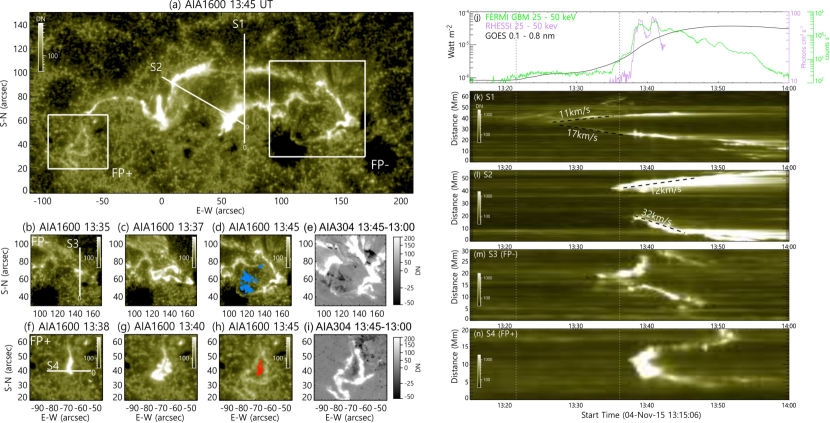
Figure 7: Formation and evolution of a flux rope’s feet (adapted from Wang et al. 2017c). Panel (a) shows the flare morphology with two irregular bright rings (marked by rectangles) attached to the far ends of flare ribbons, observed by AIA 1600 Å. The evolution of the feet associated with negative polarity (FP-) is shown in (b–e) and that associated with positive polarity (FP+) in (f–i). Panels (e and i) show coronal dimmings in 304 Å base-difference images. The dimmed pixels within FP- and FP+ are replotted in (d) and (h) in blue and red colors, respectively. Four virtual slits (S1–S4) are indicated in Panels (a), (b), and (f), with their starting points marked by ‘0’. The evolution of the flare ribbons as seen through S1 and S2 and the evolution of the bright rings as seen through slits S3 (for FP-) and S4 (for FP+) are shown in Panels (k–n), respectively. Panel (j) shows 0.1–0.8 nm flux obtained by the Geostationary Operational Environmental Satellite (GOES), 25–50 keV count rate by the Gamma-ray Burst Monitor (GBM) onboard the Fermi Gamma-ray Space Telescope, and 25–50 keV photon flux observed by the Reuven Ramaty High-Energy Solar Spectroscopic Imager (RHESSI). The 1st vertical dotted line marks the flare onset with the initial appearance of flare ribbons; the 2nd line marks the beginning of the flare main phase characterized by the rapid ribbon separation and nonthermal hard X-ray production.

5 Structure

5.1 Twist Profile

So far magnetic twist, like other characteristics of flux ropes on the Sun, can only be inferred indirectly from observation and modeling. Occasionally hard X-ray and microwave emission is observed at the projected crossing point of the kinked, inverted $\gamma$ or $\delta$-shaped filaments (Alexander et al. 2006; Liu & Alexander 2009; Cho et al. 2009; Karlický & Kliem 2010), which suggests that the their legs approach each other and interact near the crossing point. This is possible when the flux rope is highly twisted (Kliem et al. 2010; Hassanin & Kliem 2016). Vrsnak et al. (1991) measured the pitch angles of helical-shaped threads in H$\alpha$ prominences and found that the twist angles in eruptive prominences are generally larger (up to $\sim 15\pi$) than stable ones. Using the same method, Romano et al. (2003) derived that the twist angle of one helical thread in a prominence is about 10$\pi$ and relaxes to about 2$\pi$ during the eruption. Srivastava et al. (2010) estimated that a coronal loop observed in the EUV 171 Å passband possesses a twist angle of about 12$\pi$ according to the bright-dark alternating streaks along its long axis. Yan et al. (2014) inferred that the twist angle of a filament is at least 5$\pi$ based on the observed unwinding motions. Gary & Moore (2004) found an erupting four-turn helical structure observed in the UV 1600 Å passband. Since the estimated twist far exceeds the critical number of $2.5\pi$ or 1.25 turns found for a line-tying force-free flux rope with uniform twist (Hood & Priest 1981, see also § 3.2.2), the helical kink instability is suggested to be involved in these eruptions. However, it is difficult to assess to what extent one can trust such estimates of twist, because they suffer inevitably from either the projection effects or the line-of-sight confusion, in addition to complex interactions between magnetic field and plasma.

Alternatively, the magnetic field in the upper atmosphere can be constructed by NLFFF extrapolation techniques and magnetohydrostatic or magnetohydrodynamic models (see the review by Inoue 2016; Guo et al. 2017; Wiegelmann et al. 2017), based on the pre-eruption photospheric magnetic field. Flux ropes reconstructed in strong field regions tend to be moderately twisted ($\leq 2$ turns) and low lying (e.g., Régnier et al. 2002; Guo et al. 2010b; Jing et al. 2010; Inoue et al. 2011; Liu et al. 2014, 2016b; Chintzoglou et al. 2015; James et al. 2018), while those in weak-field regions tend to be highly twisted and high lying (e.g., Jiang et al. 2019; Guo et al. 2019b; Su & van Ballegooijen 2012, 2013; Su et al. 2015). In addition, the magnetic reconnection taking place at the vertical current sheet beneath an erupting flux rope will add a considerable amount of magnetic fluxes into the rope by converting overlying field to its envelope (Lin et al. 2004; Qiu et al. 2007). The post-eruption structure of the flux rope can be directly measured as a magnetic cloud by in-situ instruments on-board spacecrafts.

Revealed by various fitting and reconstruction techniques, some magnetic clouds are found to possess a large twist density, e.g., 8 turns per AU found in a magnetic cloud by Farrugia et al. (1999) and 2.4 turns per AU by Dasso et al. (2006). Wang et al. (2016b) applied a velocity-modified Gold-Hoyle model (Wang et al. 2015b) to 126 magnetic clouds, and found the distribution of twist density has a median value of about 5 turns per AU. Assuming that the cloud axial length ranges between 2–$\pi$ AU, Wang et al. (2016b) concluded that most of magnetic clouds have a twist angle significantly larger than the theoretical kink-instability threshold of $2.5\pi$ radians, but well bounded by 2 times a cylindrical rope’s aspect ratio. The total twist is subject to large uncertainties, as twist density may not be uniform along the MC field lines, whose lengths are also unknown. One way to infer the field-line length is to employ the velocity dispersion profile of in-situ energetic particles. For example, Larson et al. (1997) inferred that in a magnetic cloud the field-line length varies from about 3 AU near the edge to about 1.2 AU near the center. Expanding the study to more cases, Kahler et al. (2011) found that the field-line lengths inside magnetic clouds range between 1.3 and 3.7 AU.

Besides the local twist density, the Grad-Shafranov technique is capable of reconstructing the twist profile inside magnetic clouds (Hu & Sonnerup 2002; Hu 2017), i.e., the distribution of twist density in a cloud’s cross section. Assuming a translation symmetry along the axis, this method solves the Grad-Shafranov equation in the plane perpendicular to the flux-rope axis. Hu et al. (2014) studied twist profiles inside 18 magnetic clouds and found that about half of the cases that are associated with erupting filaments have a nearly uniform and relatively low twist, while the other half exhibit high twist ($\geq 5$ turns per AU) near the axis but low twist toward the edge. Further, Hu et al. (2015) estimated the field-line lengths based on Grad-Shafranov fitting results and found a good correlation with those estimated from the energetic electrons by Kahler et al. (2011). The measured field-line lengths are more consistent with Gold & Hoyle (1960) than Lundquist (1950) flux-rope models.

Additional insight into the twist profile inside magnetic clouds can be obtained when a magnetic cloud reconnects with the ambient interplanetary magnetic field, by which magnetic fluxes are peeled off from the cloud (McComas et al. 1994; Wei et al. 2003a; Dasso et al. 2006; Ruffenach et al. 2015). Wang et al. (2018c) studied a magnetic cloud observed sequentially by four spacecrafts near Mercury, Venus, Earth, and Mars, respectively, and found that the axial flux and helicity of the cloud decrease but its twist increases with increasing heliocentric distance. The imbalance in the azimuthal flux of the cloud at far distances implies that it has been eroded significantly. The erosion together with the increase in twist suggests that the cloud has a highly twisted core enveloped by a less twisted envelope.

Efforts have been made to compare the flux content of magnetic clouds with that of coronal flux ropes estimated from dimming signatures of eruptions (Webb et al. 2000; Mandrini et al. 2005; Attrill et al. 2006; Jian et al. 2006; Qiu et al. 2007). Post-eruption dimmings are caused by mass depletion and often appear in a pair near the flaring PIL, thus mapping the feet of the eruptive flux rope. These studies indicate a dominance of the poloidal flux over the axial flux, typically by a factor of 3 (e.g., Mandrini et al. 2005; Attrill et al. 2006; Qiu et al. 2007). However, dimming regions are often diffuse, lacking in a definite boundary. Wang et al. (2017c) made a first comparative study on the twist profile between a coronal flux rope and its interplanetary counterpart, taking advantage of a rare observation in which the rope’s feet are clearly identified and their formation starting from two brightening points during the eruption are closely monitored. Wang et al. (2017c) obtained the rope’s toroidal (axial) flux $\mathit{\Phi}_{\mathrm{t}}$ as the magnetic flux through the footpoint regions, which are identified as the conjugated coronal dimmings completely enclosed by irregular bright rings at the far ends of flare ribbons (Figure 7). The temporal variation of $\mathit{\Phi}_{\mathrm{t}}$ indicates the growth of the flux rope with time, but more importantly gives a glimpse of different ‘shells’ that build up sequentially within the rope (Figure 8). The rope’s poloidal flux $\mathit{\Phi}_{\mathrm{p}}$ can be derived from the magnetic flux swept by flare ribbons, i.e., the reconnection flux $\mathit{\Phi}_{\mathrm{r}}$ (Forbes & Priest 1984; Qiu et al. 2007). Since the flux rope in this particular case is mainly formed during the course of the eruption, $\mathit{\Phi}_{\mathrm{r}}$ may account for most of the rope’s flux, i.e., $\mathit{\Phi}_{\mathrm{r}}\approx\mathit{\Phi}_{\mathrm{p}}+\mathit{\Phi}_{\mathrm{t}}$. However, counting brightened flare area in the chromosphere gives the flux swept by both the flare ribbons and rings, denoted by $\mathit{\Phi}_{\mathrm{R}}$. It is important to keep in mind that the ribbons and the rings correspond to footpoints of topologically distinct magnetic structures: the rings highlight footpoints of the longer reconnected field lines that are newly assimilated by the burgeoning rope, therefore marking the boundary of the rope’s feet, while the ribbons represent footpoints of the shorter reconnected field lines that pile up upon the growing flare loop system. But the rings are only slightly dimmer than, and therefore cannot be distinguished from, the ribbons; as a result, $\mathit{\Phi}_{\mathrm{t}}$ is counted twice in $\mathit{\Phi}_{\mathrm{R}}$, which leads to $\mathit{\Phi}_{\mathrm{p}}\approx\mathit{\Phi}_{\mathrm{R}}-2\mathit{\Phi}_{\mathrm{t}}$.

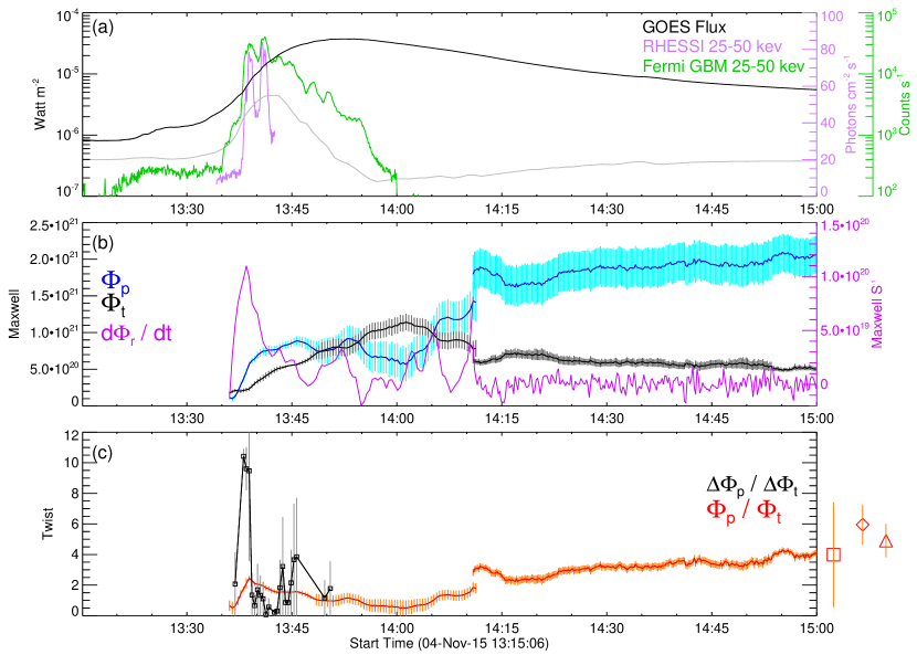
Figure 8: Temporal evolution of a flux rope in relation to the flare on 2015 November 4 (from Wang et al. 2017c). a) 0.1–0.8 nm SXR flux observed by the Geostationary Operational Environmental Satellite (GOES; black), its time derivative in an arbitrary unit (gray), and 25–50 keV HXR count rate observed by the Gamma-ray Burst Monitor (GBM) on-board the Fermi Gamma-ray Space Telescope (green) and by the Reuven Ramaty High-Energy Solar Spectroscopic Imager (RHESSI; magenta). b) Temporal evolution of poloidal flux $\mathit{\Phi}_{\mathrm{p}}$ and toroidal flux $\mathit{\Phi}_{\mathrm{t}}$ in the flux rope. Also shown is the time derivative of reconnection flux $\mathit{\Phi}_{\mathrm{r}}=\mathit{\Phi}_{\mathrm{p}}+\mathit{\Phi}_{\mathrm{t}}$. c) Temporal evolution of twist number in the flux rope as gauged by $\mathit{\Phi}_{\mathrm{p}}/\mathit{\Phi}_{\mathrm{t}}$ and $\Delta\mathit{\Phi}_{\mathrm{p}}/\Delta\mathit{\Phi}_{\mathrm{t}}$. Marked on the right are $\mathit{\Phi}_{\mathrm{p}}/\mathit{\Phi}_{\mathrm{t}}$ given by the Gold-Hoyle (square) and Lundquist (diamond) fittings and the Grad-Shafranov reconstruction (triangle) of the interplanetary magnetic cloud. .

Using $\Delta\mathit{\Phi}_{\mathrm{p}}(t)/\Delta\mathit{\Phi}_{\mathrm{t}}(t)$ to estimate the twist number at a certain shell and $\mathit{\Phi}_{\mathrm{p}}/\mathit{\Phi}_{\mathrm{t}}$ to measure the average twist number across the rope, Wang et al. (2017c) inferred that the spatial distribution of magnetic twist within the flux rope is characterized by a highly twisted core (up to about 10 turns) and less twisted outer shells (down to 1–2 turns; Figure 8c). This is corroborated by the Grad-Shafranov reconstruction of the corresponding magnetic cloud, which exhibits high twist in the center ($\sim\,$2.7 turns per AU, or, 5.4–8.5 turns given the cloud axial length ranging between 2–$\pi$ AU) and lower twist towards the boundary. Further, Wang et al. (2017c) showed similar temporal variations between $\Delta\mathit{\Phi}_{\mathrm{p}}(t)/\Delta\mathit{\Phi}_{\mathrm{t}}(t)$ (Figure 8c), the nonthermal HXR emission (Figure 8a, a proxy of both the particle and CME acceleration; Temmer et al. 2010), and the time derivative of the reconnection flux $\mathit{\Phi}_{\mathrm{r}}$ (Figure 8b, a proxy of the reconnection rate), which suggests that the instantaneous twist number may reflect the frequency of reconnections between sheared field lines, with each reconnection adding roughly one turn into the twisted field line in formation.

From theoretical perspectives, the flare ribbon morphology contains clues to the twist profile of flux ropes. Analytical models demonstrate that the photospheric footprints of the QSLs wrapping around the flux rope display two J-shaped ribbons, while the rope is anchored within the hooked parts (e.g., Démoulin et al. 1996; Titov & Démoulin 1999; Pariat & Démoulin 2012). A pair of closed hooks are associated with a flux rope of high twist numbers ($\geq 2$ turns; Démoulin et al. 1996; Pariat & Démoulin 2012), in agreement with Wang et al. (2017c), while a pair of open hooks are associated with a flux rope of moderate twist numbers ($\leq 1$ turn; Janvier et al. 2014). Twisted field lines are believed to be produced by magnetic reconnection between sheared field lines, which converts mutual to self helicity (van Ballegooijen & Martens 1989; Longcope & Beveridge 2007).

Priest & Longcope (2017) proposed that the magnetic twist builds up in the same pace as flare reconnection, which often proceeds in two phases: first the 3D “zipper reconnection” of sheared flux, which is associated with the extension of flare ribbons along the PIL, and then the quasi-2D “main phase reconnection” of unsheared flux around the flux rope, which is associated with the separation of flare ribbons away from the PIL. The zipper reconnection in a sheared arcade creates a flux rope of roughly one turn; but if starting with a preexisting flux rope under the arcade, the zipper reconnection can add substantial extra twist to the rope. Either way, the subsequent main-phase reconnection adds a layer of uniform twist of only a few turns. In this model, most of twist in the flux rope is created by zipper reconnection prior to the eruption (Threlfall et al. 2018). This is at odds with the observation made by Wang et al. (2017c, Figure 8), in which the highly twisted core is produced at around the HXR peak during the main phase rather than the zipper phase. On the other hand, motivated by Priest & Longcope (2017), Xing et al. (2020) argued that the magnetic shear angle is reflected in the geometric shear of flare ribbons, assuming a uniform distribution of magnetic flux in the area swept by flare ribbons. Applying this idea to four cases of two-ribbon flares with a preexisting flux rope but no obvious zipper ribbon motion, Xing et al. (2020) found that the preexisting rope may possess a significant amount of toroidal flux compared with that contributed by the quasi-2D reconnection during the main phase. A similar geometric argument was made by Green et al. (2011) to estimate how much flux is contributed by flux cancellation to a flux rope forming in a sigmoidal active region.

The above studies suggest that a CME flux rope builds up like an onion with nested layers of magnetic flux added sequentially as the eruption progresses, by which a non-uniform twist profile is often resulted (Hu et al. 2014; Wang et al. 2017c). Awasthi et al. (2018) brought up an alternative scenario, in which multiple flux ropes or flux bundles braid about each other and signatures of internal reconnection including nonthermal electrons, flaring plasma, and bidirectional outflowing blobs are identified. In general, a force-free flux rope embedded in potential field is expected to have a non-uniform radial twist profile to match the field at the rope surface (e.g., Török et al. 2004, their Figure 2). A quasi-separatrix layer must exist between the layers of strongly different twist. As electric currents are prone to accumulate at QSLs (§ 2.1), heating and dynamic motions are expected inside flux ropes of nonuniform twist profiles. MHD simulations of the prominence-cavity system (Xia et al. 2014; Fan 2018; Fan & Liu 2019) also reveal that there exist different types of twisted field lines threading the cavity. These field lines also possess different thermodynamic properties, therefore giving rise to the substructures of different appearances in EUV images. This may help understand disk-like or ring-like substructures observed in coronal flux ropes, even in a stable state, e.g., bright U-shaped “horns” that extend nonradially from the top of prominences (Figure 5a; Régnier et al. 2011; Schmit & Gibson 2013), hot central cores of cavities (also termed “chewy nougats”, Figure 5b; Hudson et al. 1999; Reeves et al. 2012), and nested ring-like Doppler patterns within cavities (Figure 5c; Bak-Steslicka et al. 2016).

5.2 Boundary

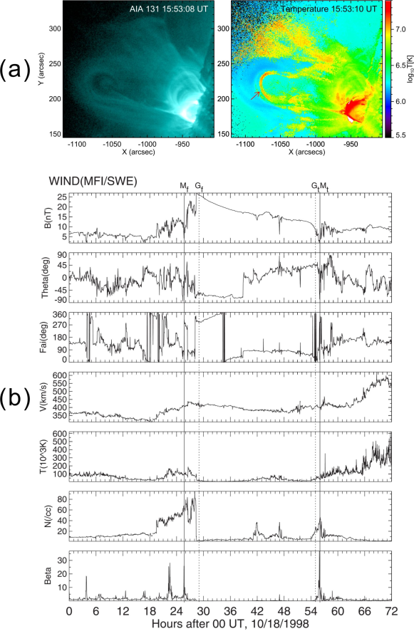
Figure 9: Boundary of erupting flux ropes observed near the Sun and in interplanetary space. a: a flux rope observed by SDO/AIA at 131 Å (left), which is enclosed by a hot shell of temperatures over 10 MK as shown in the temperature map (right; adapted from Gou et al. 2019). b: an interplanetary flux rope, also known as magnetic cloud, which is enclosed by a front and a tailing boundary layer as marked by vertical lines (adapted from Wei et al. 2003a). The boundary layers are characterized by enhanced proton temperature, proton density, and plasma $\beta$, a sudden drop in field magnitudes, and abrupt changes in field directions.

Both analytical models (e.g., Démoulin et al. 1996; Titov & Démoulin 1999; Pariat & Démoulin 2012) and numerical experiments based on NLFFF extrapolations (e.g., Guo et al. 2013; Liu et al. 2016b) or MHD simulations (e.g., Gibson & Fan 2006a; Aulanier et al. 2012; Jiang et al. 2018) have demonstrated that a coherent flux rope is wrapped around by a thin volume of strong magnetic field distortion—separatrix surfaces or QSLs that separate the twisted from untwisted fields (§ 2.1). Below we elaborate on observational signatures for the boundary of flux ropes.

For quiescent flux-rope proxies such as coronal cavities, this boundary is strongly contrasted between the dark cavity and the surrounding bright streamer (Figure 5). It is interesting that cavities appear to be more sharply defined prior to eruption (Gibson 2015). The U-shaped horn enclosing the bottom part of the cavity (Figure 5a) is thought to be associated with the HFT topology (Fan 2012).

For erupting flux ropes observed above the limb, naturally the expanding and rising flux rope would stretch and compress the overlying cold loops ($T\simeq 1-2$ MK), which pile up and subsequently become part of the erupting structure. Veronig et al. (2018) found that the outer front of these expanding and piled-up loops observed in EUV seamlessly matches with the CME front in white light. The stretched overlying loops often exhibit an $\Omega$ shape because the rising and expansion of the flux rope causes the overlying loops to curve in toward the current sheet beneath the erupting flux rope (Cheng et al. 2011b; Gou et al. 2017, 2019). Gou et al. (2019) found that when the rope’s rising speed peaks at over 500  km s^-1, a similar $\Omega$-shaped, thin layer as hot as 14–19 MK appears to separate the overlying loops from the flux rope (Figure 9a). Detailed DEM analysis shows that the layer is significantly hotter and denser than both the overlying loops and the flux rope, probably lighten up by the plasma compression as well as the current steepening and dissipation at the magnetic boundary that separates the twisted from untwisted field, which exists not only prior to but also during eruptions (e.g., Jiang et al. 2008). In the 2017 September 10 event, the erupting cavity of an inverted teardrop shape is enveloped by a hot ($T\sim 13$ MK) and dense ($\mathrm{EM}\sim 10^{27.5}$ cm^-5) layer during the early phase of the eruption, while the cavity itself has a lower emission measure ($\mathrm{EM}\sim 10^{26}$ cm^-5) and a slightly cooler temperature ($T\sim 10$ MK; Yan et al. 2018; Cheng et al. 2018b). It is interesting that the hot envelope is most prominent at the bottom part, exhibiting a U shape similar to the horn structure in quiescent cavities (Figure 5a). Underneath the cavity, the current sheet initially has the similar temperature as the cavity’s hot envelope, but is further heated to as high as 20 MK, as the flux rope propagate into the outer corona (Cheng et al. 2018b).

Regarding flux ropes erupting from the disk, the footpoint boundary of the flux rope is recognized as open or closed hooks of double J-shaped flare ribbons (Figure 7; Janvier et al. 2014; Wang et al. 2017c). The brightening at the boundary of an erupting rope’s footpoints or cross section may result either from magnetic reconnections between field lines overlying the rope, taking place at the vertical current sheet underneath the rope (Lin et al. 2004), or from reconnections between the rope and the ambient field (Shiota et al. 2010; Hassanin & Kliem 2016; Aulanier & Dudík 2019), taking place at the current sheets wrapping around the rope (Török et al. 2004; Gibson & Fan 2006a; Aulanier et al. 2010; Fan 2012, see also § 2.1).

Regarding flux ropes propagating in interplanetary space, Wei et al. (2003a) identified a boundary layer exhibiting signatures of magnetic reconnection at both the front and tail of magnetic clouds (Figure 9b). The boundary layer is characterized by a local increase in proton temperature, proton density, and plasma $\beta$, a sudden drop in field magnitudes, and abrupt changes in field directions suggesting a field reversal (Wei et al. 2003b). Tian et al. (2010) confirmed that a significant fraction of small-scale interplanetary flux ropes show boundaries of similar plasma and magnetic-field properties as those of large-scale magnetic clouds. In addition, they identified a plasma jet of $\sim\,$30  km s^-1 at the boundary, suggesting the presence of a Petschek-type reconnection exhaust (Gosling et al. 2005). These reconnection signatures could be relevant to the formation of small flux ropes in the solar wind, or, due to interactions between the flux rope and the interplanetary magnetic fields.

5.3 Double-Decker Structure

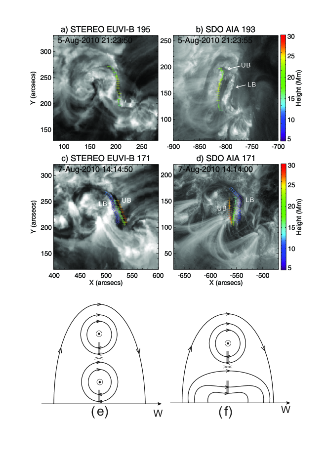
Figure 10: Double-decker filament and possible magnetic configurations (from Liu et al. 2012a). a–d) A double-decker filament observed by both STEREO-B and SDO at different dates. Selected points on the upper branch (UB) are indicated by crosses and those on the lower branch (LB) by diamonds. The heights of these points above the solar surface in units of Mm are obtained through stereoscopic triangulation and indicated by the color bar on the right. e & f) Schematic diagrams of two possible magnetic configurations for the double-decker filament in a–d. The cross sections are viewed from the south, with photospheric fields of positive (negative) polarity on the east (west) of the filament. The axial field of both filament branches points out of the plane. Slabs in gray colors indicate the filament mass. The symbol ‘x’ between the two branches marks where current sheets might develop.

As verified stereoscopically by Liu et al. (2012a), a ‘double-decker’ filament consists of two vertically separated branches that are aligned along the same PIL; it can be stable for hours to days prior to eruption (Figure 10(a–d)). The associated magnetic structure has two possible configurations, a double flux rope or a single flux rope atop a sheared arcade; the two branches, possessing the same sign of helicity, are separated by an HFT (Liu et al. 2012a, Figure 10(e & f)). The double-decker configuration may account for a long-observed puzzling phenomenon, namely, sigmoid eruptions that are survived by a stable filament (e.g., Pevtsov 2002; Liu et al. 2007a; Cheng et al. 2014b, see also § 3.1.3). This can be explained by a double decker whose lower branch embeds a filament but upper branch is avoid of filament material (Cheng et al. 2014b). As demonstrated by the NLFFF modeling of coronal magnetic field, double or even multiple flux ropes can be stacked above the same PIL (e.g., Liu et al. 2016b, 2017a; Hou et al. 2018; Awasthi et al. 2018). The other configuration, a flux rope atop a sheared arcade, is also found in NLFFF modeling (Régnier & Amari 2004) and inferred from dynamic motions i.e., rotations about the spine and longitudinal oscillations along the spine in a filament disturbed by a flare surge (Awasthi et al. 2019). In these two cases, however, the two branches possess opposite rather than same signs of helicity, which makes the tilt instability relevant (see § 3.2.3); but without the HFT in between (see also Jelínek et al. 2020), the configuration is more stable in this aspect than that originally envisaged in Liu et al. (2012a).

Double-decker filaments display a wide range of eruptive behavior. Often the upper branch is ejected as a CME while the lower branch remains confined (e.g., Liu et al. 2012a; Zhu & Alexander 2014; Cheng et al. 2014b). Additionally the two branches may erupt successively but merge into a single CME (e.g., Dhakal et al. 2018), or merge first into as a coalesced structure before eruption (e.g., Zhu et al. 2015; Tian et al. 2018). Sometimes during the slow rise phase of the upper branch, filament threads within the lower branch intermittently brighten up, lift upward, and merge into the upper branch (Liu et al. 2012a; Zhu & Alexander 2014). Since filament field is dominantly horizontal (Leroy 1989), these discrete episodes of mass transfer implies a flux transfer from the lower to the upper branch, also termed ‘flux feeding’, which may destabilize the upper branch by producing a flux imbalance in the upper branch relative to the strapping field (e.g., Su et al. 2011; Kliem et al. 2013).

Along this thought, Kliem et al. (2014b) modeled the double-decker configuration with two concentric, toroidal flux ropes, and by reducing (increasing) the flux and current in the lower (upper) rope, they were able to reproduce the ejection of the upper rope with the lower rope being stable. Alternatively, Kliem et al. (2014b) identified a double flux rope in MHD simulations of a filament eruption, in which the highly sheared core field is gradually energized through flux cancellation driven by photospheric flows. Unlike the observed double-decker filaments with two clearly separated branches (e.g., Liu et al. 2012a; Zhu & Alexander 2014), the two ropes in this simulation are initially merged to some extent until shortly before the eruption a splitting is caused by tether-cutting reconnection with the ambient field at the HFT between the two ropes. The reconnection adds flux and twist to the upper rope while strengthening the overlying flux above the lower rope, therefore leading to a partial eruption. Xia & Keppens (2016), on the other hand, focused on the internal dynamics of a twin-layer filament set up in a gravitational stratified atmosphere with dominantly horizontal magnetic field. Their three-dimensional MHD simulations demonstrate falling Rayleigh-Taylor fingers and uprising bubbles that are in line with vertical threads and rising plumes often observed in quiescent prominences, but seldom observed in double-decker filaments.

Awasthi et al. (2018) identified an even more complex system consisting of multiple flux ropes braiding about each other, morphologically similar to the braided thread-like structures observed in AIA 131 Å. Compared with a single or double flux rope, the braiding introduces a new degree of freedom as well as additional free energy, which is manifested in multi-episodes of internal reconnection. Awasthi et al. (2018) concluded that the complex ICME subsequently observed in situ derives its complexity from the source, namely, the multi-flux-rope configuration together with internal interactions.

6 Concluding Remarks

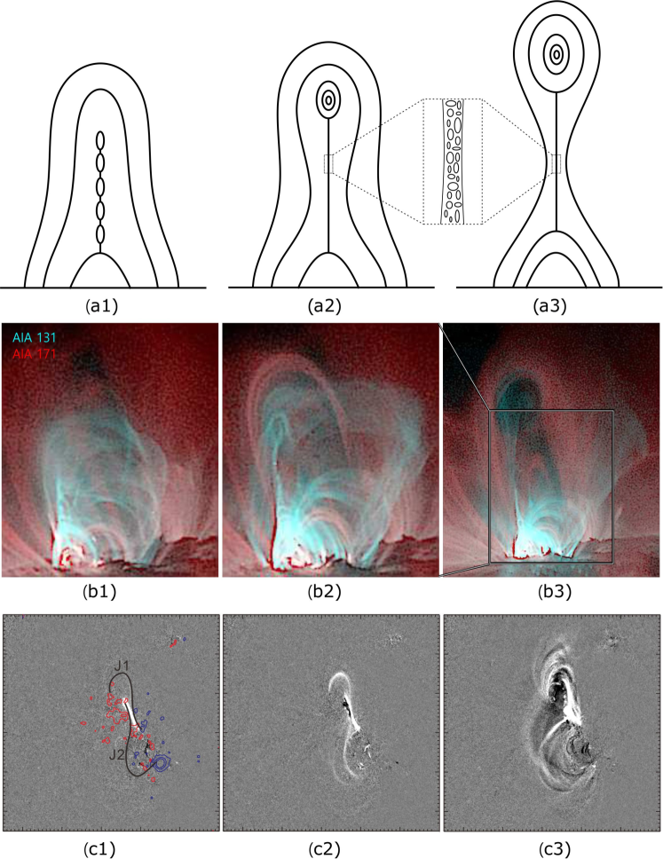
Figure 11: CME initiation through the formation a seed flux rope. (a1–a3) Schematic illustration of the CME initiation process (from Gou et al. 2019). A vertical current sheet underneath a magnetically sheared arcade breaks up into multiple plasmoids (left). The coalescence and ejection of plasmoids initiate a seed flux rope (middle), which rises and stretches the overlying field. Consequently, fast reconnection is induced at the current sheet (right), which embeds plasmoids of various scales, as illustrated by the inset. (b1–b3) Composite images of AIA 131 Å ($\sim\,$10 MK; cyan) and 171 Å ($\sim\,$0.7 MK; red) showing the initiation of the CME on 2013 May 13 (from Gou et al. 2019). The AIA images have been rotated 90 degree clockwise. The field of view in b1 and b2 is indicated by a rectangle in b3. (c1–c3) Running difference images of AIA 94 Å ($\sim\,$6 MK) showing the initiation of the CME on 2010 August 1 (adapted from Liu et al. 2010b). ‘J1’ and ‘J2’ in c1 illustrate the sheared J-shaped loops before eruption.

Magnetic flux ropes are inherently scale free. This is manifested by the wide spectrum in their size and energy in the solar atmosphere and the heliosphere. Their formation and evolution is intimately associated with flares and CMEs. Thus, the flux rope is recognized as an important agent through which it is promising to understand the physical mechanisms of, and the power-law distribution of energies in, flares and CMEs (Vourlidas et al. 2002; Yashiro et al. 2006, 2008). It has also been recognized that the formation of mini flux ropes during the spontaneous current-sheet fragmentation is key to both upward and downward cascading processes that are capable of creating a hierarchical distribution over a broad range of scales (Shibata & Tanuma 2001; Uzdensky et al. 2010; Loureiro et al. 2012; Nishizuka & Shibata 2013; Gou et al. 2019).

Recent advances combining theory, simulation, and observation have illuminated a new evolutionary path for CMEs. This picture is predicated on the formation of a vertical current sheet in a magnetically sheared arcade before the eruption, as verified in various numerical experiments (e.g., Mikic & Linker 1994; Amari et al. 1996; DeVore & Antiochos 2000; Aulanier et al. 2010). The current sheet develops as magnetic energy builds up slowly in the corona, driven by photospheric flows, and breaks up into plasmoids when its length exceeds the critical wavelength for the tearing-mode instability (Furth et al. 1963; Uzdensky et al. 2010; Bárta et al. 2011; Loureiro et al. 2012, Figure 11(a1)). Propelled by magnetic tension force, the plasmoids move along the current sheet, while neighboring plasmoids merge into larger ones due to the coalescence instability (Finn & Kaw 1977; Pritchett & Wu 1979). Upward moving plasmoids eventually merge with the leading plasmoid at the upper tip of the current sheet. A coherent flux rope, i.e., the seed CME, hence starts to form (Figure 11(a2,b2)), consistent with the appearance of a “monster” plasmoid as expected from stochastic, plasmoid-dominated reconnections (Uzdensky et al. 2010; Loureiro et al. 2012). Projected onto the disk, this seed CME may be observed in the form of an S-shaped bright loop suddenly appearing prior to the eruption (e.g., Liu et al. 2010b, Figure 11(c2)). Because of the hoop force and the upward reconnection outflows, the flux rope keeps rising to stretch the overlying field, which therefore reconnects at the current sheet as in the standard model (Lin et al. 2004, Figure 11(a3)). While the plasmoids are building up into the CME, they are simultaneously cascading into smaller scales (illustrated by the inset of Figure 11a) in a fractal fashion (Shibata & Tanuma 2001; Loureiro & Uzdensky 2016; Cheng et al. 2018b), which results in the close coupling between the flux-rope eruption and particle acceleration (e.g., Temmer et al. 2010; Gou et al. 2017, 2019, see also § 4.2.1). The observed seed CME at a meso-scale of $\sim\,$10⁸ cm is hence able to bridge the gap between the macro-scale CME ($\sim\,$10¹¹ cm near the Sun) and micro-scale (down to $\sim\,$10⁴ cm) plasmoids in the current sheet across a hierarchical spectrum.

The above picture is consistent with both statistical and case studies demonstrating that the bulk of CME flux ropes is formed by flare reconnections during eruptions (e.g., Qiu et al. 2007; Hu et al. 2014; Wang et al. 2017c); further, it has the capacity to accommodate a wide variety of plasma phenomena in the solar atmosphere. If the overlying field is strong enough, the flux-rope eruption can be confined (Török & Kliem 2005). As the flux rope temporarily settles down, a prominence may form at the bottom of the helical field lines via plasma condensation (Liu et al. 2012b; Xia et al. 2014). However, as the current sheet continues to spawn plasmoids and the plasmoids continue to merge into the flux rope, the accumulated flux in the rope may eventually reach the tipping point of eruption (Zhang et al. 2014, 2020). Additionally, whenever open field is accessible to the plasmoids, a jet may ensue instead of a CME (Shibata 1999; Sterling et al. 2015).

At this point, however, we still need a clear understanding of how small flux ropes organize themselves into a coherent, large-scale flux rope. Intimately related to this question, it is still obscure as to how a flux rope interacts with its ambient field, how neighboring flux ropes interact with each other, and how a flux rope evolves by adjusting its topology quasi-statically before, and dynamically during, the eruption. Combining high-resolution observations with data-constrained and data driven simulations will greatly help clarify these issues.

In the past few years, significant advancements have also been made in detecting signatures of flux ropes in the lower atmosphere (see the review by Wang & Liu 2019), owing primarily to meter-class ground-based telescopes represented by the 1.6-meter Goode Solar Telescope at Big Bear Solar Observatory and the 1-meter New Vacuum Solar Telescope at Fuxian Solar Observatory. These telescopes are capable of achieving the diffraction-limited spatial resolution of $\sim\,$0”.1.

In the future, coordinated multi-instrument observations will continue to be crucial in studying flux ropes on the Sun and beyond. Complemented by MHD simulations, next-generation observations obtained by the state-of-the-art instruments such as the 4-meter Daniel K. Inouye Solar Telescope, Parker Solar Probe (PSP), Solar Orbiter, as well as the Advanced Space-based Solar Observatory that is scheduled to launch in 2022 by China (ASO-S; Gan et al. 2019), will help make breakthroughs in understanding the origin, structure, and evolution of magnetic flux ropes in the solar atmosphere. In particular, PSP has a great potential to traverse CMEs with the solar activity level on the rise in the next few years. This will provide unprecedented opportunities to ‘anatomize’ flux ropes at close distances ($\gtrsim 10\ R_{\odot}$) from the Sun. This hopefully will reveal the plasma and magnetic structure of burgeoning flux ropes, in which the positive feedback between the flux-rope ejection and the magnetic reconnection is still ongoing. Meanwhile, increasingly high resolution observations, obtained by either ground-based or space-born telescopes, will continue to update our knowledge on the twisted magnetic fields in the solar atmosphere. Among these, spectral diagnostics of chromospheric and prominence magnetic fields and plasma properties are promising to provide valuable information about how twisted magnetic fields are structured and interact with plasmas in the chromospheric and coronal environment.