Magnetocaloric properties of the binary Ising model with arbitrary spin
Ümit Akıncı111umit.akinci@deu.edu.tr
Department of Physics, Dokuz Eylül University, TR-35160 Izmir, Turkey
1 Abstract
The magnetocaloric properties of the Ising binary alloys composed of arbitrary spin values, have been determined by using effective field theory. For determining the efficiency of the magnetocaloric effect in binary alloy, the quantities of interest such as isothermal magnetic entropy change and refrigerant capacity have been calculated for various values of spin and concentration. It is shown that, by changing the concentration we can tune the magnetocaloric performance. Also, it has been shown that greater refrigerant capacity can be obtained for intermediate concentration values, in comparison with the limiting concentration values.
2 Introduction
Magnetic cooling is one of the broad application areas of the magnetism. The magnetocaloric effect (MCE) [1, 2, 3, 4] allow us to use the magnetism in cooling or heating applications. If the magnetic field on the magnetic material is changed in an adiabatic way, the material can change its temperature. This is due to the balancing between the lattice (Debye term) and magnetic parts of the total entropy. Rising magnetic contribution in the total entropy change will yield decreasing the lattice contribution. This means that decreasing lattice vibrations and thus decreasing temperature. Due to the zero total entropy change (which comes from the adiabaticity of the process), by controlling magnetic part of the total entropy, one can achieve cooling or heating of the material.
There are many candidate materials of the MCE [5]. There are some parameters that determine which candidate is more efficient. Some of the parameters are isothermal magnetic entropy change (IMEC) , adiabatic temperature change ,and refrigerant capacity () , which are defined below. We can say that is still the best candidate material material for the MCE [6].
Naturally, the search for better materials still continues. Some recent developments can be found in review papers [7, 8]. Unfortunately, there are relatively small number of theoretical works devoted to the exploration of MCE for given magnetic materials. Diluted ferromagnetic systems [9], magnetic multilayers [10] quantum spin chains [11] are some of these studies.
Alloys may be good candidate materials because of the fact that, tunability of the concentration may yield obtaining material that has desired MCE properties. Some theoretical efforts have been made in this direction. For instance binary alloy [12], compound [13] , alloys [14]. Investigating alloys from a broad framework can produce important results that can be used in experiments or material science applications. Thus, the aim of this work is to determine the MCE properties of the binary alloys that can be modeled by the Ising model. The effect of the spin value (that constitute the alloy) and the concentration on the MCE properties are calculated. For this aim, the paper is organized as follows: In Sec. 3 we briefly present the model and formulation. The results and discussions are presented in Sec. 4, and finally Sec. 5 contains our conclusions.
3 Model and Formulation
The composition of the binary alloy system can be represented as . Here, the type atoms have spin value of and the concentration is , the type atoms have concentration and spin value of . The distribution of the atoms are random. The Hamiltonian of the Ising model for this system can be given as
| (1) |
where are the components of the spin- operators. The eigenvalues of these operators are . is the ferromagnetic exchange interaction between the nearest neighbor spins, is the crystal field (single ion anisotropy) and is the longitudinal magnetic field. is the site occupation number of a site , which can take values and holds. In Eq. (1), denotes the nearest neighbor pairs in the lattice.
Typical effective field approach starts by writing Hamiltonian given in Eq. (1) as single atom part () and the part that contains rest of the lattice (). Since the Hamiltonian contains only components of the spin operators, and commutes each other. Then the exact identities [15] can be used for calculation of the thermodynamic quantities
| (2) |
where represents the magnetic dipol moment per site, represents the magnetic quadrupol moment per site and so on. Here, represents the thermal average, stands for the configurational average, is the partial trace over the site , , is Boltzmann constant and is the temperature. Note that Eq. (2) contains number of equations for sublattice . This means that total number of equations is for binary alloy.
In Eq. (2), is the local field acting on site if the site has type atoms. Their expressions are as follows:
| (3) |
where represents all spin-spin interactions of atom which is the type of and it is given by
| (4) |
All operations in Eq. (2) can be done easily, since all of the matrices in that equation are diagonal. After this operation we can get the expression in a closed form as
| (5) |
where the functions for are given by [16]
| (6) |
| (7) |
Note that, as explained below, within the approximation schema used in this work there is no need to obtain functions for .
| (8) |
where represents the differential with respect to . The effect of the differential operator on an arbitrary function is given by
| (9) |
with arbitrary constant . By using from Eq. (4) in Eq. (8) we can expand the exponential differential operator by using approximated van der Waerden identities [18]. Approximated van der Waerden identities have been proposed for higher spin problems and given by
| (10) |
where and is the spin eigenvalue. This approximation equates to and to . Since we are dealing only with the quantities and , then the number of equations in Eq. (5) reduces to four. By using Eq. (10) with the identity
| (11) |
in Eq. (8), we can obtain magnetization () and quadrupolar moment () equations as
| (12) |
| (13) |
where , and
| (14) |
By solving the system of nonlinear equations given by Eqs. (12) and (13) with the coefficients given in (14) and the definitions of functions given in Eqs. (6) and (7), we can obtain the total magnetization () and quadrupolar moment () of the system as
| (15) |
The magnetocaloric performance of the magnetic system can be quantified by some quantities. The first one is IMEC when maximum applied longitudinal field is . This quantity is defined by
| (16) |
The other quantity is RC which is defined by
| (17) |
Note that, RC is amount of heat that can be transferred from the cold end (at temperature ) to the hot end (at temperature ) in one thermodynamical cycle. This measures the suitability of a magnetic material for magnetocaloric purposes. Although the chosen of these temperatures are arbitrary, in general and are chosen as those temperatures at which the magnetic entropy change gains the half of its peak value. This temperature range is defined as full width at half max (FWHM). This is also important quantity of the MCE. This three quantities will be used in this work as a magnetocaloric properties of the binary alloy.
4 Results and Discussion
The following dimensionless parameters are used in this work:
| (18) |
For a systematic investigation, we always use . This means that, rising always corresponds the rising concentration of the atoms that have lower spin value.
In our earlier work [19] we have concluded about the magnetocaloric properties of the general spin-S Ising model and they were as follows:
-
•
For a chosen external magnetic field range, the maximum value of the IMEC decreases when the spin value increases,
-
•
For a chosen external magnetic field range, the FWHM and RC increase when the spin magnitude of the system is increased,
Decreasing maximum value of the IMEC and increasing FWHM and RC by rising spin value should manifest itself in binary alloys, when decreases. For the validation of these conclusions, we depict some typical IMEC with the temperature. This behaviors can be seen in Fig. (1) for binary alloy consists of , (a) and (b) by using in Eq. (16).
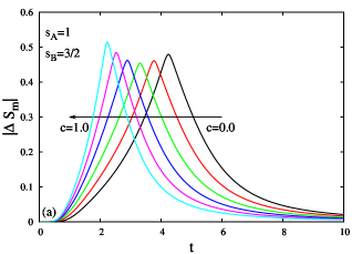
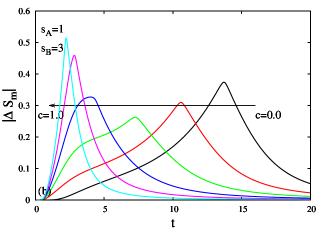
From Fig. (1), general conclusions mentioned above can be seen. But surprisingly, rising concentration () of atoms results no monotonic behavior in FWHM and the maximum value of the IMEC. For instance the maximum value of the IMEC is decreasing for a while, then increasing by rising concentration value which is starting from . This behavior is more evident for larger values of (compare Fig. (1) (b) by (a)). On the other hand, binary alloy displays broadening behavior in the variation of IMEC with the temperature, for the intermediate concentration values (see for curves related to the in Fig. (1) (b) ). We can inspect these two facts by investigation of the maximum value of the IMEC and FWHM with concentration by constructing different binary alloys, i.e. choosing different pairs.
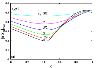
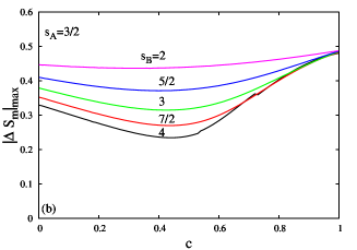
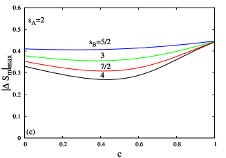
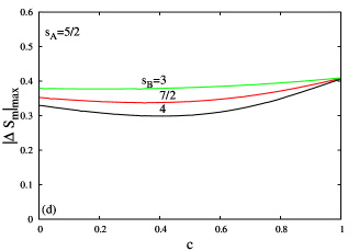
In Fig. (2) we depict the variation of the maximum value of the IMEC with the concentration for selected spin values of and . As seen in Fig. 2, the behavior of the maximum value of the IMEC by concentration is the same for all the binary alloys: rising concentration first results in decreasing behavior, then increasing behavior takes place while the concentration increases. The final value of the maximum value of the IMEC (i.e. at ) is higher than the initial value (at ) as expected [19].
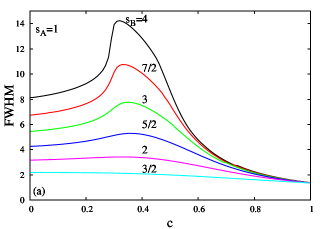
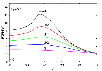
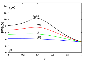
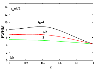
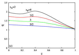
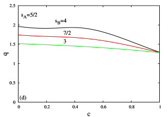
For investigation of the same behavior for FWHM we depict the variation of the FWHM with the concentration in Fig. 3, for the same binary alloys shown in Fig 2. As seen in Fig. 3, as expected again, the final value of the FWHM is lower than the initial value, when the concentration increases, for all spin pairs. But the behavior at the intermediate concentrations is again interesting. While the value of the concentration increases, first increment behavior occurs and then decreasing behavior takes place. This behavior is more evident when the binay alloy is constructed from quite different spin values (for example ).
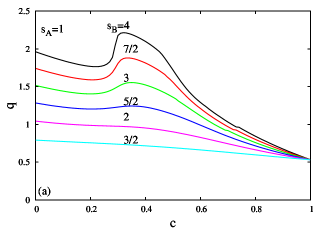
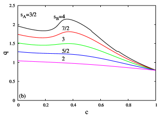
The RC is defined in Eq. (17) as the area of the portion of the IMEC curve between temperature range of FWHM. Then the behavior of the RC with the concentration is determined by behaviors of the maximum value of the IMEC and FWHM with concentration. We can see the behavior of with the concentration in Fig. 4. When we compare the behaviors depicted in Fig. 4 by behaviors given in Fig. 3 we see that the same characteristics occur. Rising concentration first rises , after then decreasing behavior occurs. Again value of is lower than the value of is compatible with the result obtained before [19].
In order to further elaborate on the investigation, we give the concentration values that makes the RC maximum in Table (1). As seen in Table (1), for some combinations, maximum RC occurs at the i.e. pure system with higher spin. But in contrast to this, for some spin combinations the maximum value of the RC occurs at the intermediate concentration values. These binary alloys are constructed by using spin values that are substantially different from each other, for instance or . This means that, the value of RC can be tuned by adjusting the concentration value.
| 3/2 | 2 | 5/2 | 3 | 7/2 | 4 | ||
| 1 | 0.00 | 0.00 | 0.00 | 0.34 | 0.32 | 0.32 | |
| 3/2 | 0.00 | 0.00 | 0.00 | 0.36 | 0.34 | ||
| 2 | 0.00 | 0.00 | 0.00 | 0.38 | |||
| 5/2 | 0.00 | 0.00 | 0.00 |
5 Conclusion
The MCE properties of the Ising binary alloys constituted from arbitrary spin values, have been determined by using effective field theory. For determining the efficiency of the MCE in binary alloy, IMEC, RC and FWHM quantities have been calculated for various values of spin and concentration.
In our earlier work we have determined the relation between the MCE properties and spin value for general spin-S Ising system [19]. Our conclusions were, when the spin value increases the maximum value of the IMEC decreases and the FWHM and RC increase. If we think only in terms of the parameter RC, we can conclude that higher spin materials are desirable in order to get more cooling power in MCE.
In this work we performed same analysis on Ising binary alloys. Two limits of the concentration values and gives the pure spin-S Ising model, i.e. these limits give the results obtained in our earlier work[19]. Surprisingly, we obtained no monotonic behavior of the properties of the MCE when the concentration changes. Perhaps most importantly, gretaer RC can be obtained for intermediate concentration values, in comparison with the limiting concentration values. This result allows the tunability of the MCE performance by changing concentration.
We hope that the results obtained in this work may be beneficial form both theoretical and experimental point of view.
References
- [1] A.M. Tishin, Y.I. Spichkin, The Magnetocaloric Effect and Its Applications, Institute of Physics, 2003.
- [2] E. Warburg, Ann. Phys. 13 (1881) 141.
- [3] P. Weiss, A. Piccard, J. Phys. (Paris) 7 (1917) 103.
- [4] P. Debye, Ann. Phys. 81 (1926) 1154.
- [5] V. Franco, J.S. Bl zquez, B. Ingale, A. Conde, Annu. Rev. Mater. Res. 42 (2012) 305.
- [6] K.A. Gschneidner Jr., V.K. Pecharsky, Annu. Rev. Mater. Sci. 30 (2000) 387.
- [7] J. Lyubina, J. Phys. D, Appl. Phys. 50 (2017) 053002.
- [8] V. Franco, J.S. Bl zquez, J.J. Ipus, J.Y. Law, L.M. Moreno-Ram rez, A. Conde, Prog. Mater. Sci. 93 (2018) 112.
- [9] K. Szalowski, T. Balcerzak, A. Bob k, J. Magn. Magn. Mater. 323 (2011) 2095.
- [10] K. Szalowski, T. Balcerzak, J. Phys. Condens. Matter 26 (2014) 386003.
- [11] M. Topilko, T. Krokhmalskii, O. Derzhko, V. Ohanyan, Eur. Phys. J. B 85 (2012) 278.
- [12] Y. Ma, A. Du, J. Magn. Magn. Mater. 321 (2009) L65.
- [13] E.P. N brega, N.A. de Oliveira, P.J. von Ranke, A. Troper, Phys. Rev. B 72 (2005) 134426.
- [14] R. Arai, R. Tamura, H. Fukuda, J. Li, A.T. Saito, S. Kaji, H. Nakagome, T. Numazawa, IOP Conf. Ser., Mater. Sci. Eng. 101 (2015) 012118.
- [15] F. C. SáBarreto, I. P. Fittipaldi, B. Zeks, Ferroelectrics 39 (1981) 1103.
- [16] J. Strecka, M. Jascur, acta physica slovaca 65 (2015) 235.
- [17] R. Honmura, T. Kaneyoshi, J. Phys. C: Solid State Phys. 12 (1979) 3979.
- [18] T. Kaneyoshi, J. Tucker, M. Jascur, Physica A 176, 495 (1992).
- [19] Ü. Akıncı Y. Yüksel, E. Vatansever Physics Letters A 382, 3238 (2018).