Storage Fit Learning with Feature Evolvable Streams

Abstract

Feature evolvable learning has been widely studied in recent years where old features will vanish and new features will emerge when learning with streams. Conventional methods usually assume that a label will be revealed after prediction at each time step. However, in practice, this assumption may not hold whereas no label will be given at most time steps. A good solution is to leverage the technique of manifold regularization to utilize the previous similar data to assist the refinement of the online model. Nevertheless, this approach needs to store all previous data which is impossible in learning with streams that arrive sequentially in large volume. Thus we need a buffer to store part of them. Considering that different devices may have different storage budgets, the learning approaches should be flexible subject to the storage budget limit. In this paper, we propose a new setting: Storage-Fit Feature-Evolvable streaming Learning (SF²EL) which incorporates the issue of rarely-provided labels into feature evolution. Our framework is able to fit its behavior for different storage budgets when learning with feature evolvable streams with unlabeled data. Besides, both theoretical and empirical results validate that our approach can preserve the merit of the original feature evolvable learning i.e., can always track the best baseline and thus perform well at any time step.

Introduction

Over the last several years, feature evolvable learning has drawn extensive attentions (Zhang et al. 2016; Hou, Zhang, and Zhou 2017a; Hou and Zhou 2018; Ye et al. 2018; Zhang et al. 2020), where old features will vanish and new features will emerge when data streams come continuously or in an online manner. There are various problem settings proposed in previous studies. For instance, in FESL (Hou, Zhang, and Zhou 2017a), there is an overlapping period where old and new features exist simultaneously when feature space switches. Hou and Zhou (2018) investigate the scenario when old features disappear, part of them will survive and continue to exist with new arriving features. Zhang et al. (2016) study that features of new samples are always equal to or larger than the old samples so as to render trapezoidal data streams. Subsequent works consider the situation that features could vary arbitrarily at different time steps under certain assumptions (Beyazit, Alagurajah, and Wu 2019; He et al. 2019).

Note that the setting of feature evolvable learning is different from transfer learning (Pan and Yang 2010) or domain adaptation (Jiang 2008; Sun, Shi, and Wu 2015). Transfer learning usually assumes that data come in batches instead of the streaming form. One exception is online transfer learning (Zhao et al. 2014) in which data from both sets of features arrive sequentially. However, they assume that all the feature spaces must appear simultaneously during the whole learning process while such an assumption does not hold in feature evolvable learning. Domain adaptation usually assumes the data distribution changes across the domains, yet the feature spaces are the same, which is evidently different from the setting of feature evolvable learning.

These conventional feature evolvable learning methods all assume that a label can be revealed in each round. However, in real applications, labels may be rarely given during the whole learning process. For example, in an object detecting system, a robot takes high-frame rate pictures to learn the name of different objects. Like a child learning in real world, the robot receives names rarely from human. Thus we will face the online semi-supervised learning problem. We focus on manifold regularization which assumes that similar samples should have the same label and has been successfully applied in many practical tasks (Zhu, Lafferty, and Rosenfeld 2005). However, this method needs to store previous samples and render a challenge on storage. Besides, different devices have different storage budget limitations, or even the available storage in the same device could be different at different times. Thus it is important to make our method adjust its behavior to fit for different storage budgets (known as storage-fit issues)  (Zhou et al. 2009; Hou, Zhang, and Zhou 2017b) which means the method should fully exploit the storage budget to optimize its performance.

In this paper, we propose a new setting: Storage-Fit Feature-Evolvable streaming Learning (SF²EL) which concerns both the lack of labels and the storage-fit issue in the feature evolvable learning scenario. We focus on FESL (Hou, Zhang, and Zhou 2017a), and other feature evolvable learning methods based on online learning technique can also adapt to our framework since our framework is not affected by specific forms of feature evolution. Due to the lack of labels, the loss function of FESL cannot be used anymore. We leverage manifold regularization technique to convert its loss function to a “risk function” without the need to consider if there exists a label or not. We also make use of a buffer strategy named reservoir sampling (Vitter 1985) when encountering the storage-fit problem. Our contributions are threefold as follows.

• Both theoretical and experimental results demonstrate that our method is able to always follow the best baseline at any time step. Thus our model can always perform well during the whole learning process in new feature space regardless of the limitation that only few data emerge in the beginning. This is a very fundamental requirement in feature evolvable learning scenario and FESL as well as other feature evolvable learning methods cannot achieve this goal when labels are barely given.

• In addition, the experimental results indicate that manifold regularization plays an important role when there are only few labels.

• Finally, we theoretically and experimentally validate that larger buffer brings better performance. Therefore, our method can fit for different storages by taking full advantage of the budget.

The rest of this paper is organized as follows. Section 2 introduces the preliminary about the basic scenario on feature evolution and the framework of our approach. Our proposed approach with two corresponding analyses is presented in Section 3. Section 4 reports experimental results. Finally, Section 5 concludes our paper.

Preliminary and Framework

We focus on binary classification task. On each round of the learning process, the learner observes an instance and gives its prediction. After the prediction has been made, with a small probability $p_{l}$, the true label is revealed. Otherwise, the instance remains unlabeled. The learner updates its predictor based on the observed instance and the label, if any. In the following, we introduce FESL that we are interested in.

FESL defines “feature space” by a set of features. And “the feature space changes” means both the underlying distribution of the feature set and the number of features change. Figure 1 illustrates how data stream comes in FESL. There are three repeating periods: in the first period a large amount of data streams come from the old feature space $S_{1}$; then in the second period named “overlapping period”, few of data come from both the old and the new feature space, i.e., $S_{1}$ and $S_{2}$; soon afterwards in the third period, data streams only come from the new feature space $S_{2}$. These three periods will continue again and again and form cycles. Each cycle merely includes two feature spaces and thus, we only need to focus on one cycle and it is easy to extend to the case with multiple cycles. Besides, FESL assumes that the old features in one cycle will vanish simultaneously according to the example of ecosystem protection where all the sensors share the same expected lifespan and thus they will wear out at the same time. The case where old features vanish asynchronously has been studied in PUFE (Hou, Zhang, and Zhou 2019), which can adapt to our framework as well.

Based on the above discussion, we only consider two feature spaces denoted by $S_{1}$ and $S_{2}$, respectively. Suppose that in the overlapping period, there are $B$ rounds of instances both from $S_{1}$ and $S_{2}$. As can be seen from Figure 1, the process can be summarized as follows.

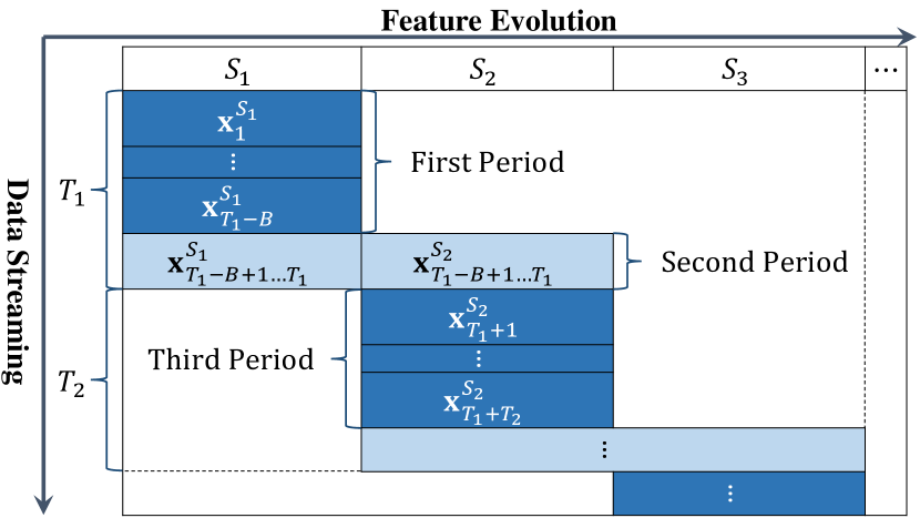
Figure 1: Illustration of how data stream comes.

• For $t=1,\ldots,T_{1}-B$, in each round, the learner observes a vector $\textbf{x}_{t}^{S_{1}}\in\mathbb{R}^{d_{1}}$ sampled from $S_{1}$ where $d_{1}$ is the number of features of $S_{1}$, $T_{1}$ is the number of total rounds in $S_{1}$.

• For $t=T_{1}-B+1,\ldots,T_{1}$, in each round, the learner observes two vectors $\textbf{x}_{t}^{S_{1}}\in\mathbb{R}^{d_{1}}$ and $\textbf{x}_{t}^{S_{2}}\in\mathbb{R}^{d_{2}}$ from $S_{1}$ and $S_{2}$ where $d_{2}$ is the number of features of $S_{2}$.

• For $t=T_{1}+1,\ldots,T_{1}+T_{2}$, in each round, the learner observes a vector $\textbf{x}_{t}^{S_{2}}\in\mathbb{R}^{d_{2}}$ sampled from $S_{2}$ where $T_{2}$ is the number of rounds in $S_{2}$. Note that $B$ is small, so we can omit the streaming data from $S_{2}$ on rounds $T_{1}-B+1,\ldots,T_{1}$ since they have minor effect on training the model in $S_{2}$.

FESL adopts linear predictor, whereas to be general, nonlinear predictor is chosen in our paper. Let $K_{i}$ denote a kernel over $\textbf{x}^{S_{i}}$ and $\mathcal{H}_{K_{i}}$ the corresponding Reproducing Kernel Hilbert Space (RKHS) (Schölkopf and Smola 2002) where $i=1,2$ that indexes the feature space. We define the projection as $\Pi_{\mathcal{H}_{K}}(b)=\operatorname*{argmin}_{\textbf{a}\in\mathcal{H}_{K}}\|a-b\|_{K}$. The predictor learned from the sequence is denoted as $f\in\mathcal{H}_{K}$. Denote by $f_{i,t},\,i=1,2$ the predictor learned from the $i$th feature space in the $t$th round. The loss function $\ell(f(\textbf{x}),y)$ is convex in its first argument such as logistic loss $\ell(f(\textbf{x}),y)=\ln(1+\exp(-yf(\textbf{x}))),$ hinge loss $\ell(f(\textbf{x}),y)=\max(0,1-yf(\textbf{x})),$ etc., for classification tasks.

If the label is fully provided, the risk suffered by the predictor in each round can be merely the prediction loss mentioned above. Then the most straightforward or baseline algorithm is to apply online gradient descent (Zinkevich 2003) on rounds $1,\ldots,T_{1}$ with streaming data $\textbf{x}_{t}^{S_{1}}$, and invoke it again on rounds $T_{1}+1,\ldots,T_{1}+T_{2}$ with streaming data $\textbf{x}_{t}^{S_{2}}$. The models are updated according to:

$$f_{i,t+1}=\Pi_{\mathcal{H}_{K_{i}}}\left(f_{i,t}-\tau_{t}\nabla\ell(f_{i,t}(\textbf{x}_{t}^{S_{i}}),y_{t})\right),\,i=1,2,$$ (1)

where $\nabla\ell(f_{i,t}(\textbf{x}_{t}^{S_{i}}),y_{t})$ is the gradient of the loss function on $f_{i,t}$ and $\tau_{t}$ is a time-varying step size, e.g., $\tau_{t}=1/\sqrt{t}$.

Nevertheless, the fundamental goal of FESL and other feature evolvable learning methods is that the model can always keep the performance at a good level no matter in the beginning of each feature space or at any other time. This baseline method cannot achieve this goal since there are only few data in the beginning of $S_{2}$ and it is difficult to obtain good performance with only training on these few data. A fundamental idea of FESL and other feature evolvable learning methods is to establish a relationship between the old feature space and the new one. In this way, the learning on the new feature space can be assisted by the old well-learned model and the goal can be achieved.

Specifically, FESL learns a mapping $\psi:\mathbb{R}^{d_{2}}\rightarrow\mathbb{R}^{d_{1}}$ between $S_{1}$ and $S_{2}$ by least squares during the overlapping period. Then when $S_{1}$ disappears, we can leverage this mapping to map the new data from $S_{2}$ into $S_{1}$ to recover the data from $S_{1}$, i.e., $\psi(\textbf{x}_{t}^{S_{2}})$. At this rate, the well-learned model $f_{1,T_{1}}$ from $S_{1}$ can make good prediction on the recovered data $\psi(\textbf{x}_{t}^{S_{2}})$ and update itself with them. Concurrently, a new model is learned in $S_{2}$ and another prediction on $\textbf{x}_{t}^{S_{2}}$ is also made. At the beginning, the $S_{1}$’s prediction $f_{1,t}(\psi(\textbf{x}_{t}^{S_{2}}))$ is good with the good predictor $f_{1,t}$ and $S_{2}$’s prediction $f_{2,t}(\textbf{x}_{t}^{S_{2}})$ is bad due to limited data. But after some time, $f_{1,t}(\psi(\textbf{x}_{t}^{S_{2}}))$ may become worse because of the cumulated error brought by the inaccurate mapping and $f_{2,t}(\textbf{x}_{t}^{S_{2}})$ will be better with more and more accurate data. FESL dynamically combines these two changing predictions with weights by calculating the loss of each base model. With this strategy, it achieves the fundamental goal in feature evolvable learning, i.e., can always follow the best base model at any time step and thus always perform well during the whole learning process in the new feature space.

Unfortunately, however, we cannot always obtain a label in each round. Thus (1) cannot be calculated so that FESL and other feature evolvable learning methods cannot achieve the goal. We leverage manifold regularization technique to mitigate this problem such that we can continue to calculate our risk function even when no labels are provided. But this operation requires the calculation of similarity between each observed sample and the current sample. This brings huge burdens on the storage and computation, which is not allowed in streaming learning or online learning scenario. Therefore, we incorporate the buffering strategy which only uses a small buffer to store representative samples. Considering that different devices provide different storage budgets, and even the same device will provide different available storages, we need to fit our method for different storages to maximize the performance (known as storage-fit issue), which can be accomplished by our buffering strategy.

So far, our framework is clear, that is:

• We first exploit manifold regularization to mitigate the problem where labels are rarely given, and then the online gradient descent can be calculated again;

• Based on the modification in the first step, we can derive our learning procedure from FESL naturally, yet with a potential problem of storage and computation;

• Finally, we use a buffering strategy to solve the storage and computation problem and subsequently solve the storage-fit issue based on this strategy.

Our Approach

Based on the framework described in the end of the last section, in this section, we introduce our approach along the way of considering “manifold regularization”, “combining base learners” and “buffering”. In the end of this section, we also provide two analyses with respect to the fundamental goal and the storage-fit issue respectively.

Manifold Regularization

With limited labels, we will face an online semi-supervised learning problem. There are several convex semi-supervised learning methods, e.g., manifold regularization and multi-view learning. Their batch risk is the sum of convex function in $f$. For these convex semi-supervised learning methods, one can derive a corresponding online semi-supervised learning algorithm using online convex programming (Goldberg, Li, and Zhu 2008). We focus on manifold regularization while the online versions of multi-view learning and other convex semi-supervised learning methods can be derived similarly.

In online learning, the learner only has access to the input sequence up to the current time. We thus define the instantaneous regularized risk $J_{i,t}(f_{i,t})$ at time $t$ to be

$$\begin{split}J_{i,t}(f_{i,t})=\frac{T}{l}\delta(y_{t})\ell(f_{i,t}(\textbf{x}_{t}^{S_{i}}),y_{t})+\frac{\lambda_{1}}{2}\|f_{i,t}\|_{K_{i}}^{2}\\ +\lambda_{2}\sum_{s=1}^{t-1}(f_{i,t}(\textbf{x}_{s}^{S_{i}})-f_{i,t}(\textbf{x}_{t}^{S_{i}}))^{2}w_{st},\,i=1,2.\end{split}$$ (2)

where $l$ is the number of labeled samples, $\ell$ is the loss function which is convex in its first argument, $f_{i,t}$ is the predictor learned in $i$th feature space and $w_{st}$ is the edge weight which defines a graph over the $T$ samples such as a fully connected graph with Gaussian weights $w_{st}=e^{-\|\textbf{x}_{s}-\textbf{x}_{t}\|^{2}/2\sigma^{2}}$. The last term in $J_{i,t}$ involves the graph edges from $\textbf{x}_{t}^{S_{i}}$ to all previous samples up to time $t$. $\frac{T}{l}$ in the first term of (2) is the empirical estimate of the inverse label probability $1/p_{l}$, which we assume is given and easily determined based on the rate at which humans can label the data at hand.

The online gradient descent algorithm applied on the instantaneous regularized risk $J_{i,t}$ will derive

$$f_{i,t+1}=\Pi_{\mathcal{H}_{k_{i}}}\left(f_{i,t}-\tau_{t}\nabla J_{i,t}(f_{i,t}(\textbf{x}_{t}^{S_{i}}))\right),\,i=1,2,$$ (3)

where $\tau_{t}$ is a time-varing step size. Thus even if no label is revealed, we can still update our model $f_{i,t}$ according to (3). Then in round $t>T_{1}$, the learner can calculate two base predictions based on models $f_{1,t}$ and $f_{2,t}$: $p_{1,t}=f_{1,t}(\psi(\textbf{x}_{t}^{S_{2}}))$ and $p_{2,t}=f_{2,t}(\textbf{x}_{t}^{S_{2}}).$ By ensemble over the two base predictions in each round, our SF²EL is able to follow the best base prediction empirically and theoretically. The initialization process to obtain the relationship mapping $\psi$ and $f_{1,T_{1}}$ during rounds $1,\ldots,T_{1}$ is summarized in Algorithm 1.

Algorithm 1 Initialize

1:  Initialize $f_{1,1}\in\mathcal{H}_{K}$ randomly;

2:  for $t=1,2,\ldots,T_{1}$ do

3:     Receive $\textbf{x}_{t}^{S_{1}}\in\mathbb{R}^{d_{1}}$ and predict $p_{t}=f_{1,t}(\textbf{x}_{t}^{S_{1}})\in\mathbb{R}$;

4:     Receive the target $y_{t}\in\mathbb{R}$ with small probability $p_{i}$, and suffer instantaneous risk $J_{i,t}$ according to (2);

5:     Update $f_{1,t}$ using (3) where $\tau_{t}=1/\sqrt{t}$;

6:     if $t>T_{1}-B$ then

7:        Learn $\psi$ by least squares;

8:     end if

9:  end for

Combining Base Learners

We propose to do ensemble by combining base learners with weights based on exponential of the cumulative risk (Cesa-Bianchi and Lugosi 2006). The prediction of our method at time $t$ is the weighted average of all the base predictions:

$$\widehat{p}_{t}=\sum_{i=1}^{2}\alpha_{i,t}p_{i,t},$$ (4)

where $\alpha_{i,t}$ is the weight of the $i$th base prediction. With the previous risk of each base model, we can update the weights of the two base models as follows:

$$\alpha_{i,t}=\frac{e^{-\eta\mathcal{J}_{i,t}}}{\sum_{j=1}^{2}e^{-\eta\mathcal{J}_{j,t}}},\,i=1,2,$$ (5)

where $\eta$ is a tuned parameter and $\mathcal{J}_{i,t}$ is the cumulative risk of the $i$th base model until time $t$: $\mathcal{J}_{i,t}=\sum_{s=1}^{t}J_{i,t},\,i=1,2.$ The risk of our predictor is calculated by

$$J_{t}=\sum_{i=1}^{2}\alpha_{i,t}J_{i,t}.$$ (6)

We can also rewrite (5) in an incremental way, which can be calculated more efficiently:

$$\alpha_{i,t+1}=\frac{\alpha_{i,t}e^{-\eta J_{i,t}}}{\sum_{j=1}^{2}\alpha_{j,t}e^{-\eta J_{i,t}}},\,i=1,2.$$ (7)

The updating rule of the weights shows that if the risk of one of the models on previous round is large, then its weight will decrease in next round, which is reasonable and can derive a good theoretical result shown in Theorem 1. Thus the procedure of our learning is that we first learn a model $f_{1,T_{1}}$ using (3) on rounds $1,\ldots,T_{1}$, during which, we also learn a relationship $\psi$ for $t=T_{1}-B+1,\ldots,T_{1}$. Then for $t=T_{1}+1,\ldots,T_{1}+T_{2}$, we learn a model $f_{2,t}$ on each round with new data $\textbf{x}_{t}^{S_{2}}$ from feature space $S_{2}$:

$$f_{2,t+1}=\Pi_{\mathcal{H}_{k_{2}}}\left(f_{2,t}-\tau_{t}\nabla J_{2,t}(f_{2,t}(\textbf{x}_{t}^{S_{2}}))\right)$$ (8)

and keep updating $f_{1,t}$ on the recovered data $\psi(\textbf{x}_{t}^{S_{2}})$:

$$f_{1,t+1}=\Pi_{\mathcal{H}_{k_{1}}}\left(f_{1,t}-\tau_{t}\nabla J_{1,t}(f_{1,t}(\psi(\textbf{x}_{t}^{S_{2}})))\right),$$ (9)

where $\tau_{t}$ is a varied step size. Then we combine the predictions of the two models by weights calculated in (7).

In order to compute (8) and (9), we first need to compute their gradients $\nabla J_{i,t}(f_{i,t}(\textbf{x}_{t}^{S_{i}})),\,i=1,2$. We express the functions in $i$th feature space $f_{i,1},\ldots,f_{i,t},\,i=1,2$ using a common set of representers $\textbf{x}_{1}^{S_{i}},\ldots,\textbf{x}_{t}^{S_{i}},\,i=1,2$, i.e.,

$$f_{i,t}=\sum_{s=1}^{t-1}\beta_{i,s}^{(t)}K_{i}(\textbf{x}_{s}^{S_{i}},\cdot),\,i=1,2.$$ (10)

To obtain $f_{i,t+1},\,i=1,2$, we need to calculate the coefficients $\beta_{i,1}^{(t+1)},\ldots,\beta_{i,t}^{(t+1)}$. We follow the kernel online semi-supervised learning approach (Goldberg, Li, and Zhu 2008) to update our coefficients by writing the gradient $\nabla J_{i,t}(f_{i,t}(\textbf{x}_{t}^{S_{i}})),\,i=1,2$ as

in which we compute the derivative according to the reproducing property of RKHS, i.e.,

$$\partial f_{i,t}(\textbf{x}_{t}^{S_{i}})/\partial f_{i,t}=\partial\langle f_{i,t},K_{i}(\textbf{x}_{t}^{S_{i}},\cdot)\rangle/\partial f_{i,t}=K_{i}(\textbf{x}_{t}^{S_{i}},\cdot),$$

where $i=1,2.$ $\ell^{\prime}$ is the (sub)gradient of the loss function $\ell$ with respect to $f_{i,t}(\textbf{x}_{t}^{S_{i}}),\,i=1,2$. Putting (11) back to (8) or (9), and replace $f_{i,t}$ with its kernel expansion (10), we can obtain the coefficients for $f_{i,t+1}$ as follows:

$$\beta_{i,s}^{(t+1)}=(1-\tau_{t}\lambda_{1})\beta_{i,s}^{(t)}-2\tau_{t}\lambda_{2}(f_{i,t}(\textbf{x}_{s}^{S_{i}})-f_{i,t}(\textbf{x}_{t}^{S_{i}}))w_{st},$$ (12)

where $i=1,2$ and $s=1,\ldots,t-1$, and

$$\begin{split}&\beta_{i,t}^{(t+1)}=2\tau_{t}\lambda_{2}\sum_{s=1}^{t-1}(f_{i,t}(\textbf{x}_{s}^{S_{i}})-f_{i,t}(\textbf{x}_{t}^{S_{i}}))w_{st}\\ &-\tau_{t}\frac{T}{l}\delta(y_{t})\ell^{\prime}(f_{i,t}(\textbf{x}_{t}^{S_{i}}),y_{t}),\,i=1,2.\end{split}$$ (13)

Buffering

As can be seen from (12) and (13), when updating the model, we need to store each observed sample and calculate the weights $w_{st}$ between the new incoming sample and all the other observed ones. These operations will bring huge burdens on computation and storage. To alleviate this problem, we do not store all the observed samples. Instead, we use a buffer to store a small part of them, which we call buffering.

We denote by $\mathcal{B}$ the buffer and let its size be $b$. In order to make the samples in buffer more representative, it is better to make each sample in the buffer sampled by equal quality. Therefore, we exploit the reservoir sampling technique (Vitter 1985) to achieve this goal which enables us to use a fixed size buffer to represent all the received samples. Specifically, when receiving a sample $\textbf{x}_{t}^{S_{i}}$, we will directly add it to the buffer if the buffer size $b>t$. Otherwise, with probability $b/t$, we update the buffer $\mathcal{B}$ by randomly replacing one sample in $\mathcal{B}$ with $\textbf{x}_{t}^{S_{i}}$. The key property of reservoir sampling is that samples in the buffer are provably sampled from the original dataset uniformly. Then the instantaneous risk will be approximated by

where the scaling factor $\frac{t-1}{b}$ keeps the magnitude of the manifold regularizer comparable to that of the unbuffered one. Accordingly, the predictor will become

$$f_{i,t}=\sum_{s\in\mathcal{B}}\beta_{i,s}^{(t)}K_{i}(\textbf{x}_{s}^{S_{i}},\cdot),\,i=1,2.$$ (15)

If the buffer size $b>t$, we will update the coefficients by (12) and (13) directly. Otherwise, if the new incoming sample replaces some sample in the buffer, there will be two steps to update our predictor. The first step is to update $f_{i,t}$ to an intermediate function $f^{\prime}$ represented by $b+1$ elements including the old buffer and the new observed sample $\textbf{x}_{t}^{S_{i}}$ as follows.

$$f^{\prime}=\sum_{s\in\mathcal{B}}\beta_{i,s}^{\prime}K_{i}(\textbf{x}_{s}^{S_{i}},\cdot)+\beta_{i,t}^{\prime}K_{i}(\textbf{x}_{t}^{S_{i}},\cdot),$$ (16)

where

$$\beta_{i,s}^{\prime}=(1-\tau_{t}\lambda_{1})\beta_{i,s}^{(t)}-2\tau_{t}\lambda_{2}(f_{i,t}(\textbf{x}_{s}^{S_{i}})-f_{i,t}(\textbf{x}_{t}^{S_{i}}))w_{st},$$ (17)

in which $i=1,2$ and $s\in\mathcal{B}$, and

$$\begin{split}&\beta_{i,t}^{\prime}=2\tau_{t}\lambda_{2}\frac{t-1}{b}\sum_{s\in\mathcal{B}}(f_{i,t}(\textbf{x}_{s}^{S_{i}})-f_{i,t}(\textbf{x}_{t}^{S_{i}}))w_{st}\\ &-\tau_{t}\frac{T}{l}\delta(y_{t})\ell^{\prime}(f_{i,t}(\textbf{x}_{t}^{S_{i}}),y_{t}),\,i=1,2.\end{split}$$ (18)

The second step is to use the newest sample $\textbf{x}_{t}^{S_{i}}$ to replace the sample selected by reservoir sampling, say $\textbf{x}_{s}^{S_{i}}$ and obtain $f_{i,t+1}$ which uses $b$ base representers by approximating $f^{\prime}$ which uses $b+1$ base representers:

$$\begin{split}\min_{\beta_{i}^{(t+1)}}\leavevmode\nobreak\ &\|f^{\prime}-f_{i,t+1}\|\\ \text{s.t.}\leavevmode\nobreak\ \leavevmode\nobreak\ \leavevmode\nobreak\ &\,f_{i,t+1}=\sum_{s\in\mathcal{B}}\beta_{i,s}^{(t+1)}K_{i}(\textbf{x}_{s}^{S_{i}},\cdot),\,i=1,2.\end{split}$$ (19)

This can be intuitively regarded as spreading the replaced weighted contribution $\beta_{i,s}^{\prime}K_{i}(\textbf{x}_{s}^{S_{i}},\cdot)$ to the remaining samples including the newly added $\beta_{i,t}^{\prime}K_{i}(\textbf{x}_{t}^{S_{i}},\cdot)$ in the buffer. The optimal $\beta_{i}^{(t+1)}$ in (19) can be efficiently found by matching pursuit (Vincent and Bengio 2002).

Algorithm 2 SF²EL

1:  Initialize $\psi$ and $f_{1,T_{1}}$ during $1,\ldots,T_{1}$ using Algorithm 1;

2:  $\alpha_{1,T_{1}}=\alpha_{2,T_{1}}=\frac{1}{2}$;

3:  Initialize $f_{2,T_{1}+1}$ randomly and $f_{1,T_{1}+1}$ by $f_{1,T_{1}}$;

4:  for $t=T_{1}+1,T_{1}+2,\ldots,T_{1}+T_{2}$ do

5:     Receive $\textbf{x}_{t}^{S_{2}}\in\mathbb{R}^{S_{2}}$;

6:     Predict $p_{1,t}=f_{1,t}(\psi(\textbf{x}_{t}^{S_{2}}))\;\text{and}\;p_{2,t}=f_{2,t}(\textbf{x}_{t}^{S_{2}})$;

7:     Predict $\widehat{p}_{t}\in\mathbb{R}$ using (4);

8:     Receive the target $y_{t}\in\mathbb{R}$ with small probability $p_{i}$, and suffer instantaneous risk $J_{t}$ according to (6);

9:     Update base predictions’ weights using (7);

10:     Update $f_{1,t}$ and $f_{2,t}$ using (9) and (8) respectively with buffering strategy in Section Buffering where $\tau_{t}=1/\sqrt{t-T_{1}}$.

11:  end for

If the new incoming sample does not replace the sample in the buffer, $f_{i,t+1}$ will still consist of the representers from the unchanged buffer. Then only the coefficients of the representers from the buffer will be updated as follows.

$$\beta_{i,s}^{(t+1)}=(1-\tau_{t}\lambda_{1})\beta_{i,s}^{(t)}-2\tau_{t}\lambda_{2}(f_{i,t}(\textbf{x}_{s}^{S_{i}})-f_{i,t}(\textbf{x}_{t}^{S_{i}})),$$ (20)

where $i=1,2$ and $s\in\mathcal{B}$.

Algorithm 2 summarizes our SF²EL.

Analysis

In this section, we borrow regret from online learning to measure the performance of SF²EL. Specifically, we give a risk bound which demonstrates that the performance will be improved with the assistance of the old feature space. We define that $\mathcal{J}^{S_{1}}$ and $\mathcal{J}^{S_{2}}$ are two cumulative risks suffered by base models on rounds $T_{1}+1,\ldots,T_{1}+T_{2}$, $\mathcal{J}^{S_{1}}=\sum_{t=T_{1}+1}^{T_{1}+T_{2}}J_{1,t}$, $\mathcal{J}^{S_{2}}=\sum_{t=T_{1}+1}^{T_{1}+T_{2}}J_{2,t},$ and $\mathcal{J}^{S_{12}}$ is the cumulative risk suffered by our method according to the definition of our predictor’s risk in (6): $\mathcal{J}^{S_{12}}=\sum_{t=T_{1}+1}^{T_{1}+T_{2}}J_{t}.$ Then we have (proof is deferred to supplementary file):

Theorem 1.

Assume that the risk function $J_{t}$ takes value in [0,1]. For all $T_{2}>1$ and for all $y_{t}\in\mathcal{Y}$ with $t=T_{1}+1,\ldots,T_{1}+T_{2}$, $\mathcal{J}^{S_{12}}$ with parameter $\eta=\sqrt{\ln 2/T_{2}}$ satisfies

$$\mathcal{J}^{S_{12}}\leq\min(\mathcal{J}^{S_{1}},\mathcal{J}^{S_{2}})+\sqrt{T_{2}\ln 2}.$$ (21)

Remark 1.

This theorem implies that the cumulative risk $\mathcal{J}^{S_{12}}$ of Algorithm 2 over rounds $T_{1}+1,\ldots,T_{1}+T_{2}$ is comparable to the minimum of $\mathcal{J}^{S_{1}}$ and $\mathcal{J}^{S_{2}}$. Furthermore, we define $C=\sqrt{T_{2}\ln 2}$. If $\mathcal{J}^{S_{2}}-\mathcal{J}^{S_{1}}>C$, it is easy to verify that $\mathcal{J}^{S_{12}}$ is smaller than $\mathcal{J}^{S_{2}}$. In summary, on rounds $T_{1}+1,\ldots,T_{1}+T_{2}$, when $f_{1,t}$ is better than $f_{2,t}$ to certain degree, the model with assistance from $S_{1}$ is better than that without assistance.

Furthermore, we prove that larger buffer can bring better performance by leveraging our buffering strategy. Concretely, let $R_{t}$ be the last term of the objective (2), which is formed by all the observed samples till the current iteration. Denote by $\hat{R}_{t}$ the approximated version formed by the observed samples in the buffer. Then we have:

Theorem 2.

With the reservoir sampling mechanism, the approximated objective is an unbiased estimation of objective formed by the original data, namely, $\mathbb{E}[R_{t}]=\mathbb{E}[\hat{R}_{t}]$.

Remark 2.

Theorem 2 demonstrates the rationality of the reservoir sampling mechanism in buffering. The objective formed by the observed samples in the buffer is provably unbiased to that formed by all the observed samples. Furthermore, the variance of the approximated objective will decrease with more observed samples in a larger buffer, leading to a more accurate approximation, which suggests us to make the best of the buffer storage to store previous observed samples. Since various devices have different storage budgets and even the same device will provide different available storages, we can fit our method for different storages to maximize the performance by taking full advantage of the budget. This proof can be found in supplementary file.

Experiments

In this section, we conduct experiments in different scenarios to validate the three claims presented in Introduction.

Compared Methods

We compare our SF²EL to $7$ baseline methods:

• NOGD: (Naive Online Gradient Descent): mentioned in Preliminary, where once the feature space changes, the online gradient descent algorithm will be invoked from scratch.

• uROGD (updating Recovered Online Gradient Descent): utilizes the model learned from feature space $S_{1}$ by online gradient descent to do predictions on the recovered data and keeps updating with the recovered data.

• fROGD (fixed Recovered Online Gradient Descent): also utilizes the model learned from $S_{1}$ to do predictions on the recovered data like uROGD but keeps fixed.

• NOGD+MR: NOGD boosted by manifold regularization (MR).

• uROGD+MR: uROGD boosted by MR.

• fROGD+MR: fROGD boosted by MR.

• FESL-Variant: FESL (Hou, Zhang, and Zhou 2017a) cannot be directly applied in our setting. For fair comparison, we modify the original FESL to a non-linear version which only updates on the rounds when there is a label revealed. FESL-Variant is actually the SF²EL without MR.

Note that NOGD, uROGD, fROGD and FESL-Variant do not update on rounds when no label is revealed while NOGD+MR, uROGD+MR, fROGD+MR and our SF²EL keep updating on every round. We want to emphasize that it is sufficient to validate the effectiveness of our framework by merely comparing our method to these baselines mentioned above in the scenario of FESL since our goal is: (1) our model can be comparable to these base models, (2) the manifold regularization is useful and (3) our method can fit for the storage budget to maximize its performance. With the manifold regularization and buffering strategy, other feature evolvable learning methods based on the online learning technique can also adapt to our framework similarly.

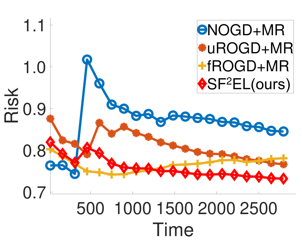
  (a) Credit-a

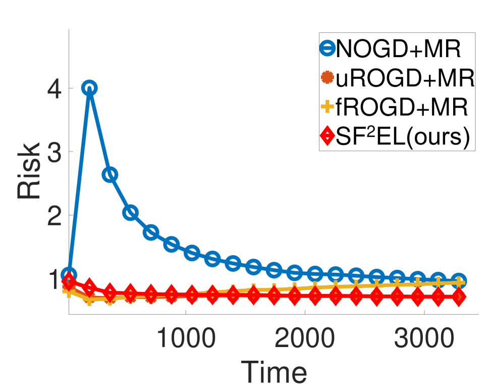
  (b) Diabetes

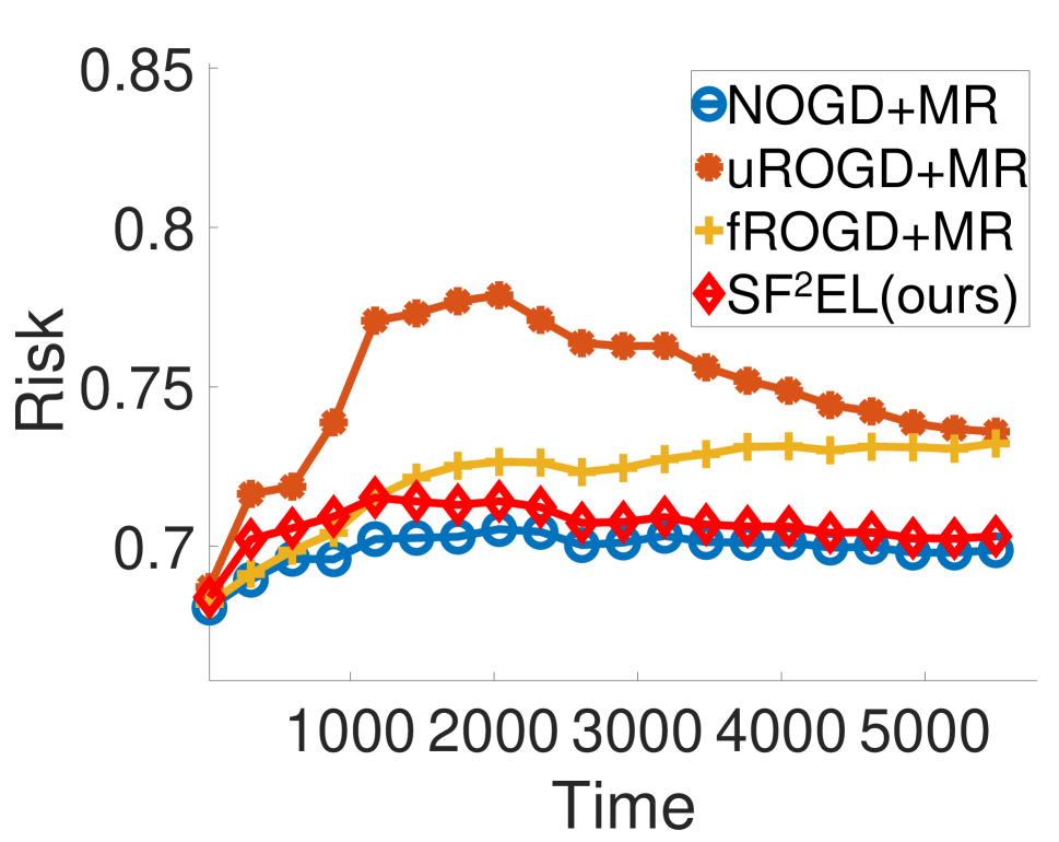
  (c) Svmguide3

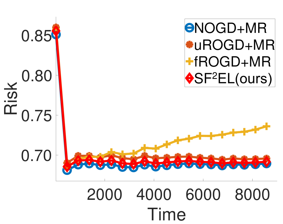
  (d) Swiss

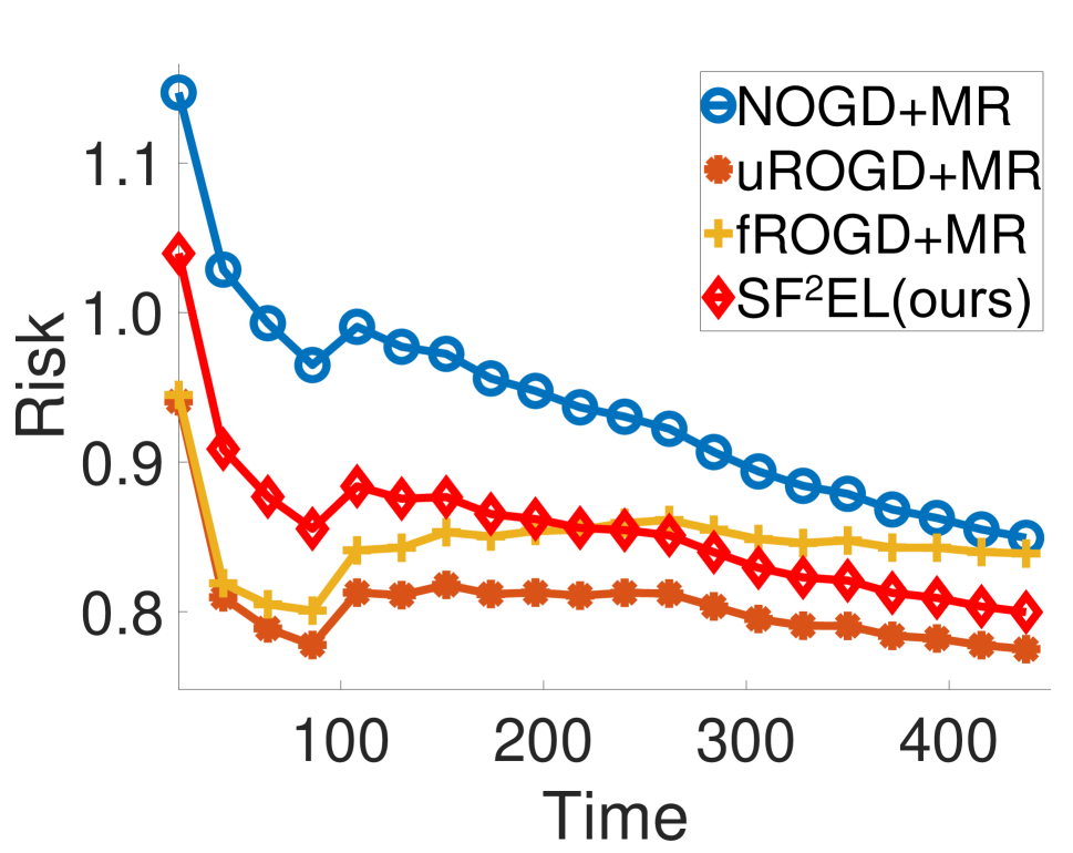
  (e) RFID

Figure 2: The trend of risk with NOGD+MR, uROGD+MR, fROGD+MR and SF²EL. We only compare SF²EL with these baselines because those without MR cannot calculate a risk when there is no label. The smaller the cumulative risk is, the better. All the average cumulative risk at any time of our method is comparable to the best baselines. Note that our goal is to be comparable to the best baseline and is not necessary to be better than them. fROGD+MR’s risk sometimes increases because it does not update itself.

Table 1: Accuracy (mean$\pm$std) comparisons between baselines and SF²EL when buffer size is $60$. “+MR” means the baselines are boosted by manifold regularization(MR). Better result in each grid is marked by $\bullet$. The best one among all the methods is bold. Note that our goal is to be comparable to the best baseline and is not necessary to be better than them.

Dataset	Credit-a	Diabetes	Svmguide3	Swiss	RFID	HTRU_2	magic04
NOGD	.690$\pm$.051	.643$\pm$.029	.657$\pm$.036	.711$\pm$.044	.687$\pm$.042	.885$\pm$.022	.580$\pm$.120
NOGD+MR	$\bullet$.706$\pm$.049	$\bullet$.672$\pm$.019	$\bullet$.668$\pm$.037	$\bullet$.807$\pm$.026	$\bullet$.688$\pm$.042	$\bullet$ .907$\pm$.001	$\bullet$.616$\pm$.058
uROGD	.740$\pm$.038	.658$\pm$.021	.675$\pm$.045	.694$\pm$.071	.571$\pm$.036	.943$\pm$.014	.550$\pm$.172
uROGD+MR	$\bullet$.760$\pm$.034	$\bullet$.678$\pm$.015	$\bullet$.680$\pm$.048	$\bullet$.824$\pm$.050	$\bullet$.572$\pm$.036	$\bullet$.944$\pm$.010	$\bullet$.603$\pm$.079
fROGD	.672$\pm$.087	.633$\pm$.056	.648$\pm$.035	.702$\pm$.073	.560$\pm$.045	.757$\pm$.179	.550$\pm$.172
fROGD+MR	$\bullet$.697$\pm$.079	$\bullet$.654$\pm$.041	$\bullet$.659$\pm$.037	$\bullet$ .811$\pm$.067	$\bullet$.561$\pm$.045	$\bullet$.943$\pm$.020	$\bullet$.649$\pm$.001
FESL-Variant	.759$\pm$.028	.666$\pm$.018	.686$\pm$.039	.855$\pm$.034	.688$\pm$.040	.885$\pm$.022	.556$\pm$.162
SF2EL (ours)	$\bullet$.768$\pm$.029	$\bullet$.685$\pm$.011	$\bullet$.694$\pm$.040	$\bullet$.939$\pm$.020	$\bullet$.690$\pm$.040	$\bullet$.912$\pm$.008	$\bullet$.649$\pm$.001

Evaluation and Parameter Setting

We evaluate the empirical performances of the proposed approaches on classification task on rounds $T_{1}+1,\ldots,T_{1}+T_{2}$. We assume all the labels can be obtained in hindsight. Thus the accuracy is calculated on all rounds. Besides, to verify that Theorem 1 is reasonable, we present the trend of average cumulative risk. Concretely, at each time $t^{\prime}$, the risk $\bar{J}_{i,t^{\prime}}$ of every method is the average of the cumulative risk over $1,\ldots,t^{\prime}$, namely $\bar{J}_{i,t^{\prime}}=(1/t^{\prime})\sum\nolimits_{t=1}^{t^{\prime}}J_{i,t}$. The probability of labeled data $p_{l}$ is set as $0.3$. We also conduct experiments on other different $p_{l}$ and our SF²EL also works well. The performances of all approaches are obtained by average results over $10$ independent runs.

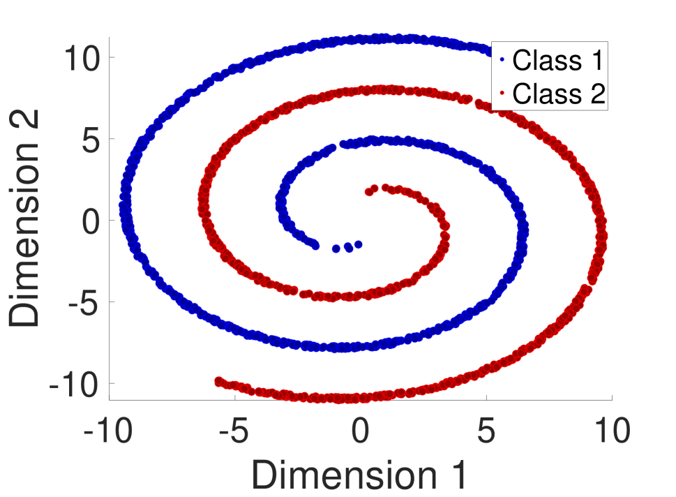
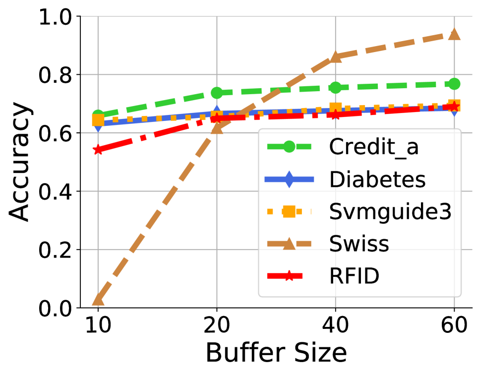
Figure 3: (a) is the manifold of Swiss dataset. (b) exhibits the impact of buffer size on accuracy.

Datasets

We conduct our experiments on $7$ datasets from different domains including economy and biology, etc. Note that in FESL $30$ datasets are used. However, over $20$ of them are the texting datasets which do not satisfy the manifold characteristic. The datasets used in our paper all satisfy the manifold characteristic and the Swiss dataset (like a swiss roll) is the perfect one. Swiss is a synthetic dataset containing $2000$ samples and is generated by two twisted spiral datasets. As Swiss has only two dimensions, it is convenient for us to observe its manifold characteristic. As can be seen from Figure 3, Swiss satisfies a pretty nice manifold property. Other datasets used in our paper also have such property but as a matter of high dimension, we only use Swiss as an example. To generate synthetic data of feature space $S_{2}$, we artificially map the original datasets by random matrices. Then we have data both from feature space $S_{1}$ and $S_{2}$. Since the original data are in batch mode, we manually make them come sequentially. In this way, synthetic data are completely generated. As for the real dataset, we use “RFID” dataset provided by FESL which satisfies all the assumptions in Preliminary. “HTRU_2” and “magic04” are two large-scale datasets which contain $17898$ and $19020$ instances respectively and we only provide their accuracy results in Table 1 due to page limitation. Other results on these two datasets can be found in the supplementary file.

Results

We have three claims mentioned in Introduction. The first is that our method can always follow the best baseline at any time and thus achieve the fundamental goal of feature evolvable learning: always keeps the performance at a good level. The second is that manifold regularization brings better performance when there are only a few labels. The last one is that larger buffer will bring better performance and thus our method can fit for different storages by taking full advantage of the budget. In the following, we show the experimental results that validate these three claims.

Following the Best Baseline

Figure 2 shows the trend of risk of our method and the baselines boosted by manifold regularization. We only compare SF²EL with baselines boosted by MR because those without MR cannot calculate a risk when there is no label. The smaller the cumulative risk is, the better. fROGD+MR’s risk sometimes increases because it does not update itself. Note that our goal is let our model be comparable to the best baseline yet is not necessary to be better than them. We can see that our method’s risk is always comparable with the best baseline which validates Theorem 1. And surprisingly, as can be seen from Table 1, our method’s accuracy results on classification tasks almost outperform those of the baseline methods ($6$ out of $7$).

MR Brings Better Performance

In Table 1, we can see that MR makes NOGD, fROGD and uROGD better, and our method also benefits from it. Specifically, our SF²EL is based on the ensemble of uROGD+MR and NOGD+MR, which makes it the best in all datasets. FESL-Variant is based on NOGD and uROGD. Although it is better than NOGD and uROGD, it is worse than our SF²EL.

Table 2: Accuracy (mean$\pm$std) comparisons with different buffer sizes. The best ones among all the buffers are bold. We can find that larger buffer brings better performance.

Buffer	Credit-a	Diabetes	Svmguide3	Swiss	RFID
10	.659$\pm$.052	.631$\pm$.066	.644$\pm$.103	.290$\pm$.070	.542$\pm$.056
20	.737$\pm$.036	.666$\pm$.025	.655$\pm$.064	.617$\pm$.067	.650$\pm$.059
40	.755$\pm$.039	.676$\pm$.016	.683$\pm$.034	.861$\pm$.031	.662$\pm$.054
60	.768$\pm$.029	.685$\pm$.011	.694$\pm$.040	.939$\pm$.020	.690$\pm$.040

Storage Fit

Figure 3 and Table 2 provides the performance comparisons between different buffer sizes from both the perspective of numerical values and figure. We can see that larger buffer brings better performance which validates Theorem 2. With this regard, our method SF²EL can fit for different storages to maximize the performance by taking full advantage of the budget. We can also see that the Swiss dataset which possesses the best manifold property enjoys most the increasing of the buffer size.

Conclusion

Learning with feature evolvable streams usually assumes that a label can be revealed immediately in each round. However, in reality this assumption may not hold. We introduce manifold regularization into FESL and let FESL work well in this scenario. Other feature evolvable learning can also adapt to our framework. Both theoretical and experimental results validate that our method can follow the best baselines and thus work well at any time step. Besides, we theoretically and empirically demonstrate that a larger buffer can bring better performance and thus our method can fit for different storages by taking full advantage of the budget.

Appendix: Supplementary Materials

In the supplementary materials, we will prove the two theorems presented in the section “Our Approach”, and provide the details of the datasets that used in our paper and additional experimental results on two large datasets.

Analysis

In this section, we will give the detailed proofs of the two theorems in the section “Our Approach”.

Proof of Theorem 1

Proof.

In order to prove Theorem 1, we first introduce potential function $\Phi_{t}=\frac{1}{\eta}\ln\left(\sum_{i=1}^{2}\exp(-\eta\mathcal{J}_{i,t})\right)$. Then we have

$$\Phi_{t}-\Phi_{t-1} =\frac{1}{\eta}\ln\left(\frac{\sum_{i=1}^{2}\exp(-\eta\mathcal{J}_{i,t})}{\sum_{i=1}^{2}\exp(-\eta\mathcal{J}_{i,t-1})}\right)$$

$$=\frac{1}{\eta}\left(\sum_{i=1}^{2}\alpha_{i,t}\exp(-\eta J_{i,t})\right)$$

$$\quad\quad(e^{-y}\leq 1-y+y^{2}\,\text{for all}\,y\geq 0)$$

$$\leq\frac{1}{\eta}\left(\sum_{i=1}^{2}\alpha_{i,t}(1-\eta J_{i,t}+\eta^{2}J_{i,t}^{2})\right)$$

$$=\frac{1}{\eta}\ln\left(1-\eta\sum_{i=1}^{2}\alpha_{i,t}J_{i,t}+\eta^{2}\sum_{i=1}^{2}\alpha_{i,t}J_{i,t}^{2}\right)$$

$$\quad\quad(\ln(1+y)\leq y)$$

$$\leq-\sum_{i=1}^{2}\alpha_{i,t}J_{i,t}+\eta\sum_{i=1}^{2}\alpha_{i,t}J_{i,t}^{2}$$

Summing over $t=T_{1}+1,\ldots,T_{1}+T_{2}$, letting $\mathcal{J}_{i,T_{1}}=0$, telescoping and rearranging give

$$\sum_{t=T_{1}+1}^{T_{1}+T_{2}}\alpha_{i,t}J_{i,t} \leq\Phi_{T_{1}}-\Phi_{T_{1}+T_{2}}+\eta\sum_{t=T_{1}+1}^{T_{1}+T_{2}}\alpha_{i,t}J_{i,t}^{2}$$

$$\leq\frac{\ln 2}{\eta}-\frac{1}{\eta}\ln(\exp(-\eta\mathcal{J}_{i^{\star},T_{1}+T_{2}}))$$

$$\quad\quad+\eta\sum_{t=T_{1}+1}^{T_{1}+T_{2}}\sum_{i=1}^{2}\alpha_{i,t}J_{i,t}^{2}$$

$$\leq\frac{\ln 2}{\eta}+\mathcal{J}_{i^{\star},T_{1}+T_{2}}+\eta\sum_{t=T_{1}+1}^{T_{1}+T_{2}}\sum_{i=1}^{2}\alpha_{i,t}J_{i,t},$$

where

$$\sum_{t=T_{1}+1}^{T_{1}+T_{2}}\alpha_{i,t}J_{i,t}=\mathcal{J}^{S_{12}}$$

and

$$\mathcal{J}_{i^{\star},T_{1}+T_{2}}=\min(\mathcal{J}^{S_{1}},\mathcal{J}^{S_{2}}).$$

Considering the boundness of $J_{t}$, thus we have

$$\mathcal{J}^{S_{12}}\leq\min(\mathcal{J}^{S_{1}},\mathcal{J}^{S_{2}})+\frac{\ln 2}{\eta}+T_{2}\eta.$$ (22)

When $\eta$ is optimally set to $\sqrt{\ln 2/T_{2}}$, (21) can be immediately derived. ∎

Proof of Theorem 2

Proof.

The proof of this theorem can be derived simply by using induction.
Basis:

$i=k:\,\textbf{Pr}(\textbf{x}_{t}\in\mathcal{B}_{t})=\frac{b}{t}$, where $\mathcal{B}_{t}$ is the $\mathcal{B}$ in $t$-th step.
Induction $t\rightarrow t+1$:

• Assume our first $t$ elements have been chosen with probability $\frac{b}{t}$.

• The algorithm chooses the $i+1$-th element with probability $\frac{b}{t+1}$.

• If we choose this element, each element in $\mathcal{B}_{t}$ has probability $\frac{1}{b}$ of being replaced.

• The probability that an element in $\mathcal{B}_{t}$ is replaced with the $t+1$-th element is therefore $\frac{1}{b}\frac{b}{t+1}=\frac{1}{t+1}$.

• Thus the probability of an element not being replaced is $1-\frac{1}{t+1}=\frac{t}{t+1}$.

• So $\mathcal{B}_{t+1}$ contains any given element either because it was chosen into $\mathcal{B}_{t}$ and not replaced: $\textbf{Pr}(\textbf{x}_{t}\in\mathcal{B}_{t+1})=\frac{b}{t}\frac{t}{t+1}=\frac{b}{t+1}$.

• Or because it was chosen in the latest round with probability $\frac{b}{t+1}$.

We already prove that each element in $\mathcal{B}$ at time step $t$ is sampled with equal quality $p_{s\in\mathcal{B}}=\frac{b}{t}$. Then we have

$$\mathbb{E}[R_{t}] =\sum_{s=1}^{t-1}\mathbb{E}[r_{s}]=\sum_{s=1}^{t-1}\sum_{k\in\mathcal{B}_{t}}p_{k}r_{k}$$

$$=(t-1)\sum_{k\in\mathcal{B}_{t}}p_{k}r_{k}=\frac{t-1}{b}b\sum_{k\in\mathcal{B}_{t}}p_{k}r_{k}$$

$$=\frac{t-1}{b}\sum_{s\in\mathcal{B}_{t}}\sum_{k\in\mathcal{B}_{t}}p_{k}r_{k}=\frac{t-1}{b}\sum_{s\in\mathcal{B}_{t}}\mathbb{E}[r_{s}]$$

$$=\mathbb{E}\left[\frac{t-1}{b}\sum_{s\in\mathcal{B}_{t}}r_{s}\right]=\mathbb{E}[\hat{R}_{t}]$$

where $r_{s}=f_{i,t}(\textbf{x}_{s}^{S_{i}})-f_{i,t}(\textbf{x}_{t}^{S_{i}}))^{2}w_{st},\,i=1,2$.

∎

Datasets

In the following, we present the details of all the datasets we used in our paper. The information of dimensions is presented in Table 3 where $n$ is the number of instances, $d_{1}$ is the number of features of the feature space $S_{1}$, and $d_{2}$ is the number of features of the feature space $S_{2}$. It is worth noting that RFID is a real dataset.

Table 3: The dimensions of the datasets.

Dataset	$n$	$d_{1}$	$d_{2}$
Credit-a	653	15	10
Diabetes	768	8	5
Svmguide3	1,284	22	15
Swiss	2000	2	3
RFID	940	78	72
HTRU_2	17898	8	5
magic04	19020	10	7

The descriptions and the sources of the datasets in our experiment are as follows:

• Credit_a: this dataset concerns credit card applications. All attribute names and values have been changed to meaningless symbols to protect confidentiality of the data. Credit_a can be found in https://archive.ics.uci.edu/ml/datasets/Credit+Approval.

• Diabetes: this dataset consists of diabetes patients data and is from https://archive.ics.uci.edu/ml/datasets/diabetes.

• Svmguide3: this dataset is from (hsu2003practical) and can be accessed via https://www.csie.ntu.edu.tw/~cjlin/libsvmtools/datasets/binary.html.

• Swiss: this dataset is a synthetic dataset containing 2000 samples and is generated by two twisted spiral datasets. As Swiss has only two dimensions, it is convenient for us to observe its manifold characteristic.

• RFID: this dataset is a real dataset from (Hou, Zhang, and Zhou 2017a). The authors used the RFID technique to collect the real data which contains 450 samples from $S_{1}$ and $S_{2}$ respectively. In this dataset, the RFID technique is used to predict the location’s coordinate of the moving goods attached by RFID tags. RFID dataset is from http://www.lamda.nju.edu.cn/data˙RFID.ashx.

• HTRU_2: this dataset describes a sample of pulsar candidates collected during the High Time Resolution Universe Survey (South). It can be obtained from https://archive.ics.uci.edu/ml/datasets/HTRU2.

• magic04: the data are MC generated to simulate registration of high energy gamma particles in a ground-based atmospheric Cherenkov gamma telescope using the imaging technique. You can get this dataset from https://archive.ics.uci.edu/ml/datasets/magic+gamma+telescope.

Additional Experiments

In this section, we provide the additional experimental results on the two large datasets HTRU_2 and magic04.

Note that we have three claims mentioned in Introduction. The first is that our method can always follow the best baseline at any time and thus achieve the fundamental goal of feature evolvable learning: always keeps the performance at a good level. The second is that manifold regularization brings better performance when there are only a few labels. The last one is that larger buffer will bring better performance and thus our method can fit for different storages by taking full advantage of the budget.

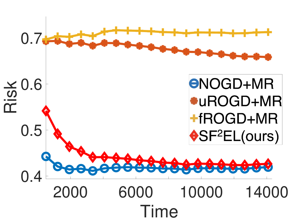
  (a) HTRU_2

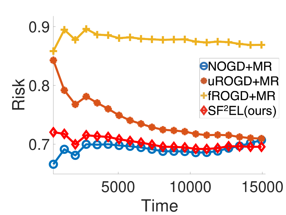
  (b) magic04

Figure 4: The trend of risk with NOGD+MR, uROGD+MR, fROGD+MR and SF²EL on large-scale datasets HTRU_2 and magic04. The smaller the cumulative risk is, the better. All the average cumulative risk at any time of our method is comparable to the best baselines.

The numerical accuracy comparisons of the two large datasets have been exhibited in Table 1 in the main body. Figure 4 shows the trend of risk of our method and the baselines boosted by manifold regularization. We only compare SF²EL with baselines boosted by MR because those without MR cannot calculate a risk when there is no label. The smaller the cumulative risk is, the better. Similar with the results illustrated in Figure 2 in the main body, on these two large datasets, fROGD+MR’s risk sometimes increases because it does not update itself. Note that our goal is let our model be comparable to the best baseline yet is not necessary to be better than them. We can see that our method’s risk on the two large datasets is always comparable with the best baseline which validates Theorem 1.

Table 4: Accuracy (mean$\pm$std) comparisons with different buffer sizes on large-scale datasets HTRU_2 and magic04. The best ones among all the buffers are bold. We can find that larger buffer brings better performance.

Buffer	HTRU_2	magic04
10	.890$\pm$.029	.559$\pm$.053
20	.906$\pm$.003	.589$\pm$.036
40	.907$\pm$.002	.601$\pm$.061
60	.912$\pm$.008	.641$\pm$.026

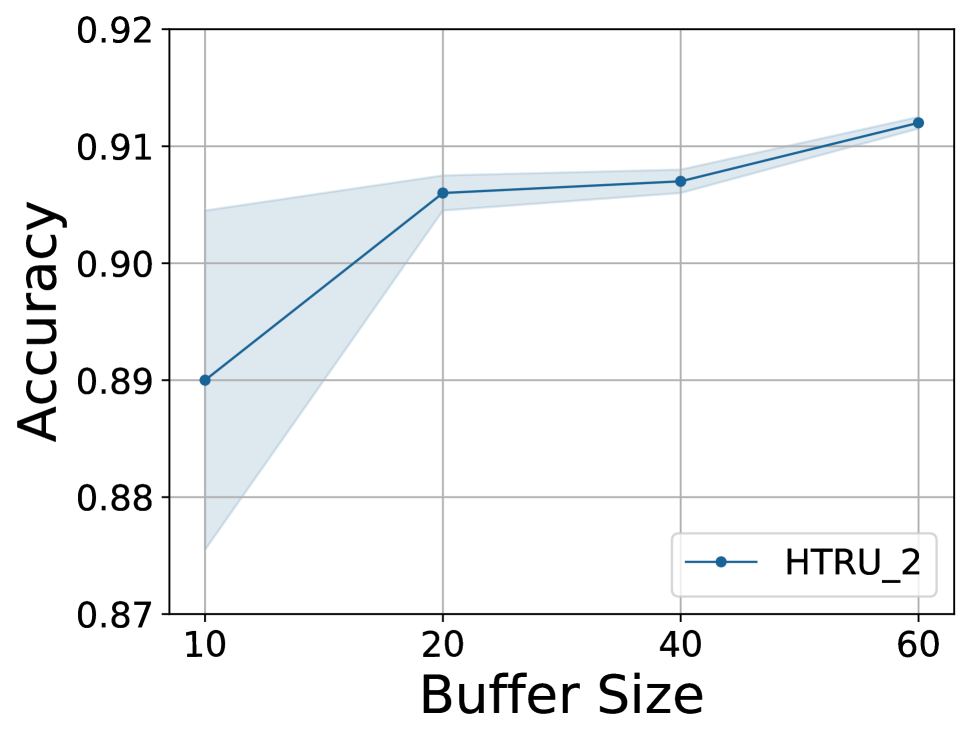
  (a) HTRU_2

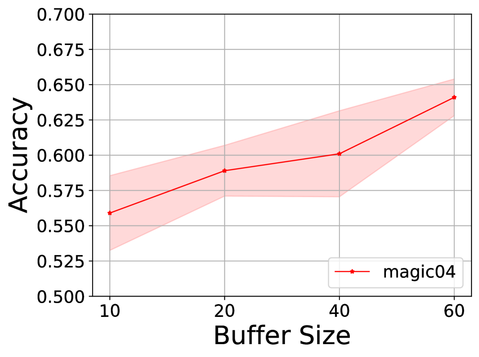
  (b) magic04

Figure 5: The impact of buffer size on accuracy on large datasets HTRU_2 and magic04.

Table 4 and Figure 5 provide the performance comparisons between different buffer sizes from both the perspective of numerical values and figure. We can see that similar with the results shown in Table 2 and Figure 3 in the main body, larger buffer brings better performance which validates Theorem 2. With this regard, our method SF²EL can fit for different storages to maximize the performance by taking full advantage of the budget.

References

- Beyazit, Alagurajah, and Wu (2019) Beyazit, E.; Alagurajah, J.; and Wu, X. 2019. Online Learning from Data Streams with Varying Feature Spaces. In Proceedings of the 33rd AAAI Conference on Artificial Intelligence, 3232–3239.
- Cesa-Bianchi and Lugosi (2006) Cesa-Bianchi, N.; and Lugosi, G. 2006. Prediction, Learning, and Games. Cambridge University Press.
- Goldberg, Li, and Zhu (2008) Goldberg, A. B.; Li, M.; and Zhu, X. 2008. Online Manifold Regularization: A New Learning Setting and Empirical Study. In Proceedings of the 19th European Conference on Machine Learning and Principles of Knowledge Discovery in Databases, 393–407.
- He et al. (2019) He, Y.; Wu, B.; Wu, D.; Beyazit, E.; Chen, S.; and Wu, X. 2019. Online Learning from Capricious Data Streams: A Generative Approach. In Proceedings of the 28th International Joint Conference on Artificial Intelligence, 2491–2497.
- Hou, Zhang, and Zhou (2017a) Hou, B.-J.; Zhang, L.; and Zhou, Z.-H. 2017a. Learning with Feature Evolvable Streams. In Advances in Neural Information Processing Systems 30, 1417–1427.
- Hou, Zhang, and Zhou (2017b) Hou, B.-J.; Zhang, L.; and Zhou, Z.-H. 2017b. Storage Fit Learning with Unlabeled Data. In Proceedings of the 26th International Joint Conference on Artificial Intelligence, 1844–1850.
- Hou, Zhang, and Zhou (2019) Hou, B.-J.; Zhang, L.; and Zhou, Z.-H. 2019. Prediction with Unpredictable Feature Evolution. CoRR abs/1904.12171.
- Hou and Zhou (2018) Hou, C.; and Zhou, Z.-H. 2018. One-Pass Learning with Incremental and Decremental Features. IEEE Transactions on Pattern Analysis and Machine Intelligence 40(11): 2776–2792.
- Jiang (2008) Jiang, J. 2008. A literature survey on domain adaptation of statistical classifiers. URL: http://sifaka. cs. uiuc. edu/jiang4/domainadaptation/survey 3: 1–12.
- Pan and Yang (2010) Pan, S. J.; and Yang, Q. 2010. A Survey on Transfer Learning. IEEE Transactions on Knowledge and Data Engineering 22: 1345–1359.
- Schölkopf and Smola (2002) Schölkopf, B.; and Smola, A. J. 2002. Learning with Kernels: support vector machines, regularization, optimization, and beyond. Adaptive computation and machine learning series. MIT Press.
- Sun, Shi, and Wu (2015) Sun, S.; Shi, H.; and Wu, Y. 2015. A survey of multi-source domain adaptation. Information Fusion 24: 84–92.
- Vincent and Bengio (2002) Vincent, P.; and Bengio, Y. 2002. Kernel Matching Pursuit. Machine Learning 48(1-3): 165–187.
- Vitter (1985) Vitter, J. S. 1985. Random Sampling with a Reservoir. ACM Transactions on Mathematical Software 11(1): 37–57.
- Ye et al. (2018) Ye, H.-J.; Zhan, D.-C.; Jiang, Y.; and Zhou, Z.-H. 2018. Rectify Heterogeneous Models with Semantic Mapping. In Proceedings of the 35th International Conference on Machine Learning, 1904–1913.
- Zhang et al. (2016) Zhang, Q.; Zhang, P.; Long, G.; Ding, W.; Zhang, C.; and Wu, X. 2016. Online Learning from Trapezoidal Data Streams. IEEE Transactions on Knowledge and Data Engineering 28: 2709–2723.
- Zhang et al. (2020) Zhang, Z.-Y.; Zhao, P.; Jiang, Y.; and Zhou, Z.-H. 2020. Learning with Feature and Distribution Evolvable Streams. In Proceedings of the 37th International Conference on Machine Learning, 11317–11327.
- Zhao et al. (2014) Zhao, P.; Hoi, S.; Wang, J.; and Li, B. 2014. Online Transfer Learning. Artificial Intelligence 216: 76–102.
- Zhou et al. (2009) Zhou, Z.-H.; Ng, M. K.; She, Q.-Q.; and Jiang, Y. 2009. Budget Semi-supervised Learning. In Proceedings of 13th Pacific-Asia Conference on Knowledge Discovery and Data Mining, 588–595.
- Zhu, Lafferty, and Rosenfeld (2005) Zhu, X.; Lafferty, J.; and Rosenfeld, R. 2005. Semi-supervised learning with graphs. Ph.D. thesis, Carnegie Mellon University, language technologies institute, school of computer science.
- Zinkevich (2003) Zinkevich, M. 2003. Online Convex Programming and Generalized Infinitesimal Gradient Ascent. In Proceedings of the 20th International Conference on Machine Learning, 928–936.