Fast Graphlet Transform of Sparse Graphs

Abstract

We introduce the computational problem of graphlet transform of a sparse graph. Graphlets are fundamental topology elements of all graphs/networks. They can be used as coding elements to encode graph-topological information at multiple granularity levels, for classifying vertices on the same graph/network, as well as, for making differentiation or connection across different networks. Network/graph analysis using graphlets has growing applications. We recognize the universality and increased encoding capacity in using multiple graphlets, we address the arising computational complexity issues, and we present a fast method for exact graphlet transform. The fast graphlet transform establishes a few remarkable records at once in high computational efficiency, low memory consumption, and ready translation to high-performance program and implementation. It is intended to enable and advance network/graph analysis with graphlets, and to introduce the relatively new analysis apparatus to graph theory, high-performance graph computation, and broader applications.

I Introduction

$\boldsymbol{\sigma}_{\mathbf{0}}$

$\boldsymbol{\sigma}_{\mathbf{4}}$

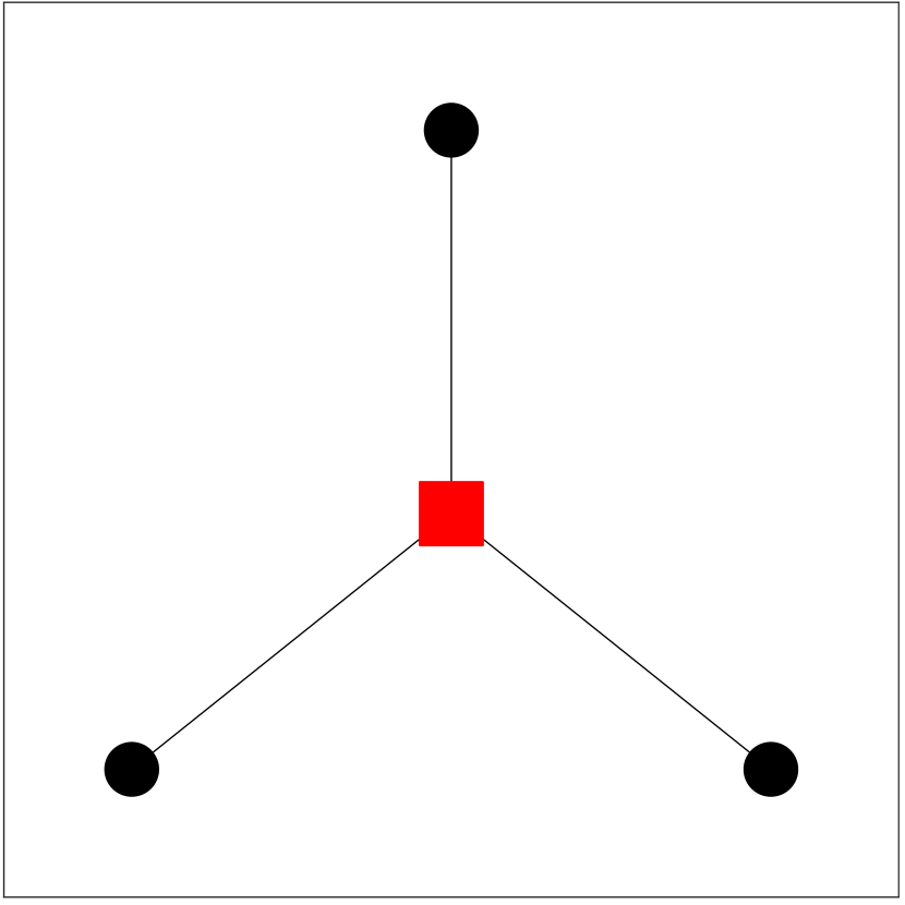
$\boldsymbol{\sigma}_{\mathbf{8}}$

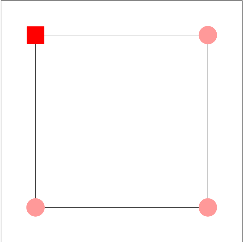
$\boldsymbol{\sigma}_{\mathbf{12}}$

$\boldsymbol{\sigma}_{\mathbf{1}}$

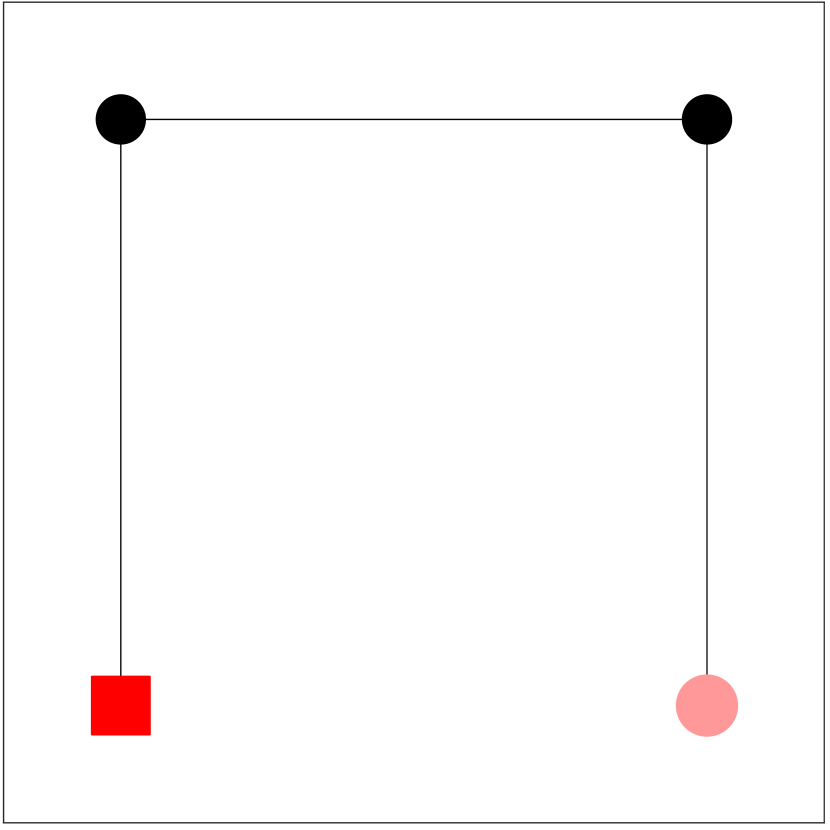
$\boldsymbol{\sigma}_{\mathbf{5}}$

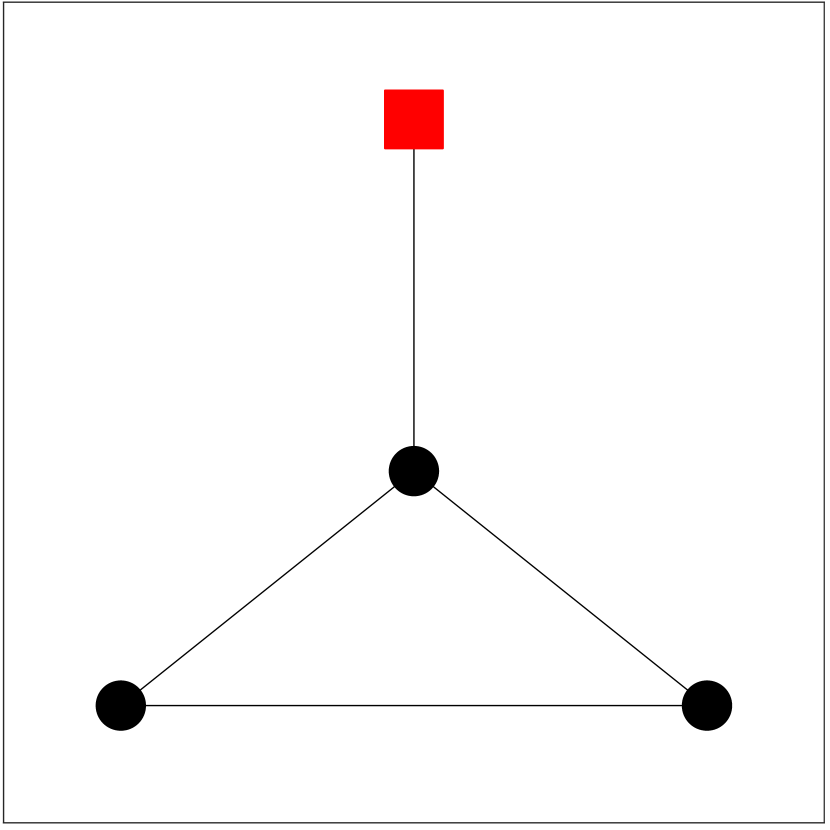
$\boldsymbol{\sigma}_{\mathbf{9}}$

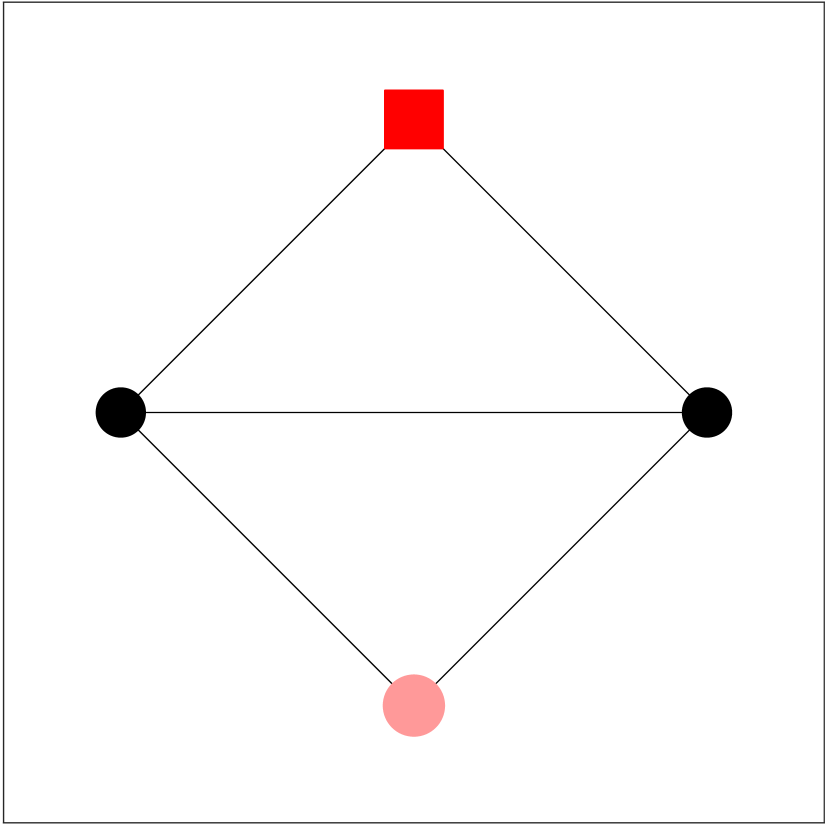
$\boldsymbol{\sigma}_{\mathbf{13}}$

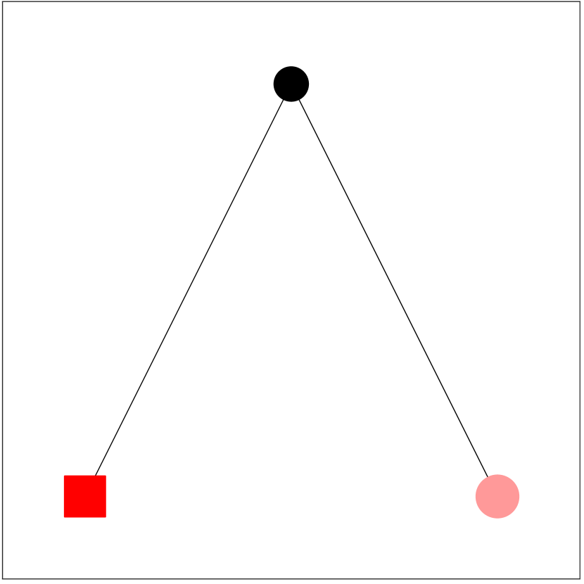
$\boldsymbol{\sigma}_{\mathbf{2}}$

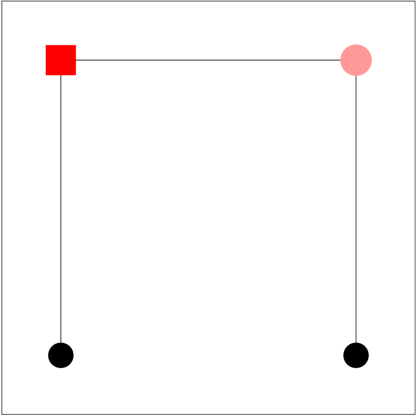
$\boldsymbol{\sigma}_{\mathbf{6}}$

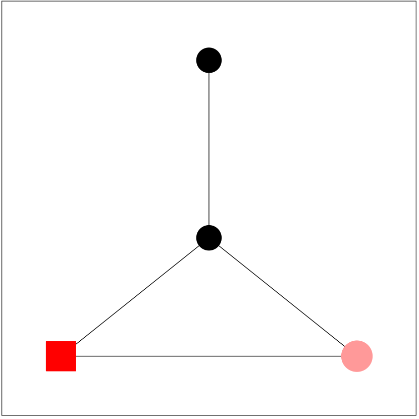
$\boldsymbol{\sigma}_{\mathbf{10}}$

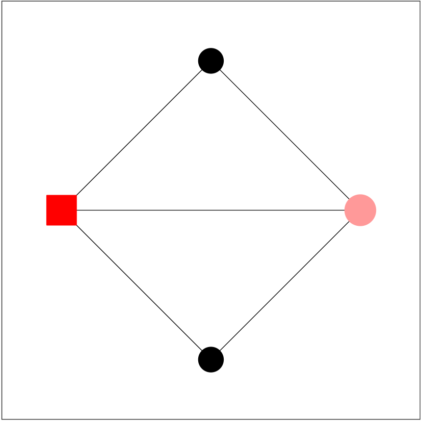
$\boldsymbol{\sigma}_{\mathbf{14}}$

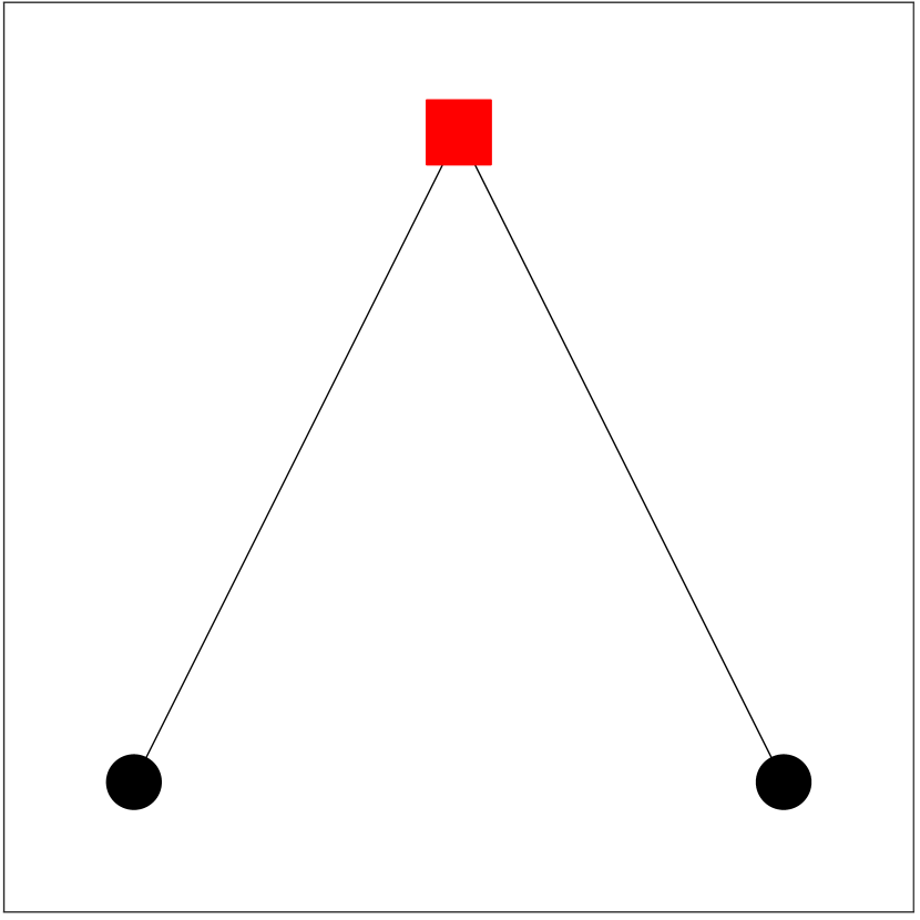
$\boldsymbol{\sigma}_{\mathbf{3}}$

$\boldsymbol{\sigma}_{\mathbf{7}}$

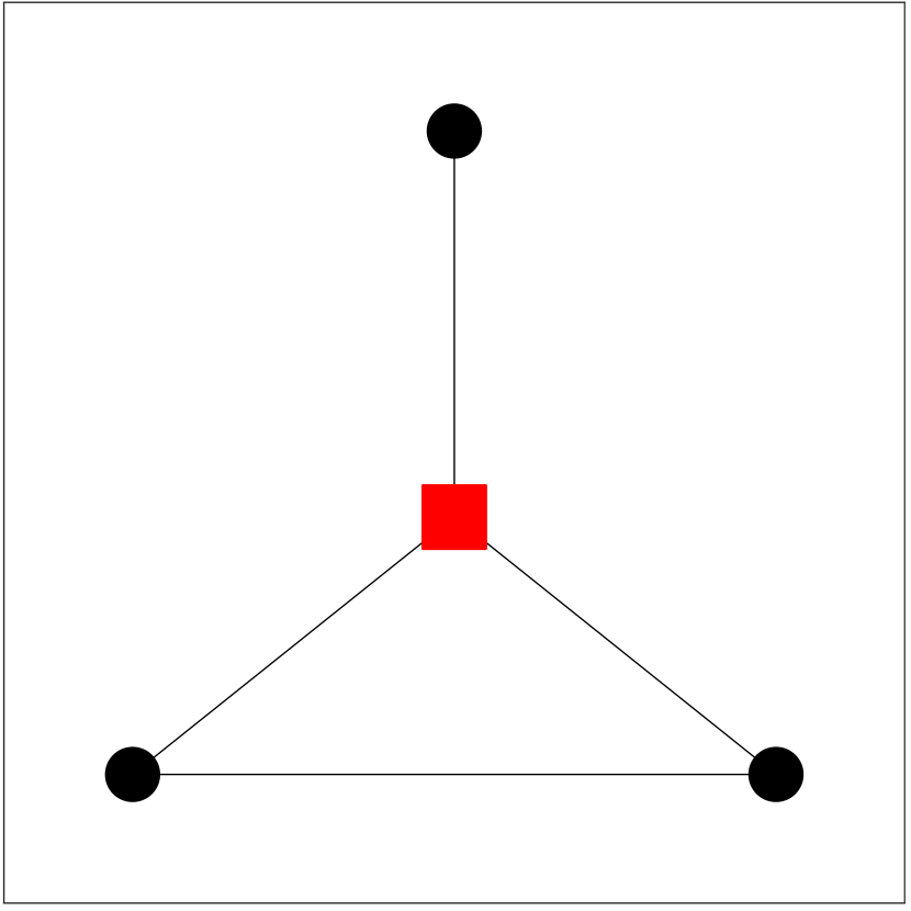
$\boldsymbol{\sigma}_{\mathbf{11}}$

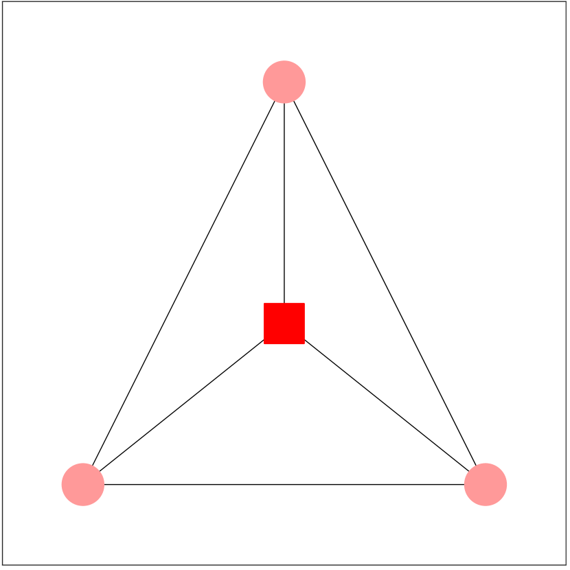
$\boldsymbol{\sigma}_{\mathbf{15}}$

Figure 1: Dictionary $\Sigma_{16}$ of $16$ graphlets. In each graphlet, the designated incidence node is specified by the red square marker, its automorphic position(s) specified by red circles. The total ordering (labeling) of the graphlets is by the following nesting conditions. The graphlets are ordered first by non-decreasing number of vertices. Graphlets with the same vertex set belong to the same family. Within each family, the ordering is by non-decreasing number of edges, and then by increasing degree at the incidence node (except the $4$-cycle). The inclusion of $\sigma_{0}$ is necessary to certain vertex partition analysis [7].

Network analysis using graphlets has advanced in recent years. The concepts of graphlets, graphlet frequency, and graphlet analysis are originally introduced in 2004 by Pržulj, Corneil and Jurisica [17]. They have been substantially extended in a number of ways [28, 21, 24, 13, 26]. Graphlets are mostly used for statistical characterization and modeling of entire networks. In the work by Palla et. al. [15], which is followed by many, a network of motifs (a special case of graphlets) is induced for overlapping community detection on the original network. Recently we established a new way of using graphlets for graph analysis. We use graphlets as coding elements to encode topological and statistical information of a graph at multiple granularity levels, from micro-scale structures at vertex neighborhoods, up to macro-scale structures such as cluster configurations [7]. We also use the topology encoded information to uncover temporal patterns of variation and persistence across networks in a time-shifted sequence, not necessarily over the same vertex set [8].

We anticipate a growing interest in, and applications of, graphlet-based network/graph analysis, for the following reasons. Graphlets are fundamental topology elements of all networks or graphs. See a particular graphlet dictionary shown in Fig. 1. Conceptually, graphlets for network/graph analysis are similar to wavelets for spectro-temporal analysis in signal processing [20], shapelets for time series classification [29], super-pixels for image analysis [19], and n-grams for natural language processing [22, 23]. Like motifs, graphlets are small graphs. By conventional definition, motifs are small subgraph patterns that appear presumptively and significantly more frequently in a network under study. Motif analysis relies on prior knowledge or assumption [11]. Graphlets are ubiquitous; graphlet analysis reveals the most frequent connection patterns or motifs, or lack of dominance by any, in a network.

There is another aspect of the universality in using graphlets. Graphlets are defined in the graph-topology space. They are not to be confused with the wavelets applied to the spectral elements of a particular graph Laplacian as in certain algebraic graph analysis. The latter is limited to the family of graphs defined on the same vertex set and share the same eigenvectors. Otherwise, the Laplacians of two graphs on the same vertex set are not commutable. The computation of Laplacian spectral values and vectors is also limited, by complexity and resources, to low-dimensional invariant subspaces. Graphlets hold a promise to overcome the limitation.

The time and space complexities of graph encoding with graphlets, i.e., the graphlet transform, have not been formally described and addressed. The transform with encoding dictionary $\Sigma$, to be described in Section II, maps graph $G=(V,E)$ to a $|V|\times|\Sigma|$ array of graphlet frequencies at all vertices. In fact, the mapping is related to the classical problem of finding, classifying and counting small subgraphs over vertex neighborhoods [18, 6]. A familiar case is to find and count all triangles over the entire graph. The triangle is graphlet $\sigma_{4}$ ($C_{3},K_{3}$) in Fig. 1. With the graphlet transform, the number/frequency of distinct triangles incident on each and every vertex is computed. It is found, from an analysis of scientific collaboration networks [8], that the bi-fork graphlet $\sigma_{3}$ ($K_{1,2}$) encodes the betweenness among triangle clusters. Another familiar case is to find and count induced claw subgraphs, the claw is graphlet $\sigma_{8}$ ($K_{1,3}$). The naive method checks every connected quad-node subgraph for claw recognition. Its time complexity is $O(n^{4})$, $n=|V|$. The naive method can be accelerated by applying fast matrix multiplication algorithms on asymptotically sufficiently large graphs, at the expense of greater algorithmic complication, and if feasible to implement, with increased memory consumption, loss of data locality and increased latency in memory access on any modern computer with hierarchical memory. There is another type of counting methods that search the patterned subgraphs from neighborhood to neighborhood, with detailed book keeping [4, 10]. Due to the high computational complexity, certain network analysis with graphlets resorts to nondeterministic approximation with sparse sampling under a structure-persistent assumption [18]. Otherwise, it is known that certain network properties are not preserved with sampling [25].

This work makes a few key contributions. We formally introduce the graphlet transform problem, and address the issues with encoding capacity and complexity. We present sparse and fast formulas for the graphlet transform of any large, sparse graph, with any sub-dictionary of $\Sigma_{16}$ as the coding basis. The transform is deterministic, exact and directly applicable to any range of graph size. Our solution method establishes remarkable records at once in multiple aspects – time complexity, memory space complexity, program complexity and high-performance implementation. Particularly, the time complexity of the fast graphlet transform with any dictionary $\Sigma\!\subseteq\!\Sigma_{16}$ is linear in $(|V|+|E|)|\Sigma|$ on degree-bounded graphs or planar graphs. Contrary to existing methods, the transform formulas can be straightforwardly translated to high performance computation[9], via the use of readily available software libraries such as GraphBLAS [5]. We also address criteria of selecting graphlet elements for certain counting-based decision or detection problems on graphs. This work serves twofold objectives: to enable large network/graph analysis with graphlets and to enrich and advance sparse graph theory, computation and their applications.

The basic assumptions and notations throughout the rest of the paper are as follows. Graph $G=(V,E)$ has $n=|V|$ nodes/vertices and $m=|E|$ edges/links. It is sparse, such as $m=O(n\log^{k}n)$ with a small value of $k$. The nodes are indexed from $1$ to $n$, a particular ordering is specified when necessary. Graph $G$ is simple, undirected and specified by its (symmetric) adjacency matrix $A$ of 0-1 values. The $j$-th column of $A$, denoted by $a_{j}$, marks the neighbors of node $j$. Denote by $e_{j}$ the $j$-th column of the identity matrix. The sum of all $e_{j}$ is the constant-1 vector, denoted by $e$. The maximal degree is $d_{\max}$. The Hadamard (elementwise) multiplication is denoted by $\odot$. The number of nonzero elements in matrix $B$ is $\mathrm{nnz}(B)$. The total number of arithmetic operations for constructing $B$ is $\mathrm{cost}(B)$. For any two non-negative matrices $A$ and $B$, $A\!-\!B$ is the shorthand expression for the sparse difference, i.e., the elementwise rectified difference $\max\{A-B,0\}$.

II Graphlet transform: problem description

We now describe generic graphlets and graphlet dictionaries by their forms and attributes, with modification in description over the original, for clarity. A graphlet is a connected graph with a small vertex set and a unique orbit ( a subset of vertices symmetric under permutations). We show in Fig. 1 a dictionary of $16$ graphlets, $\Sigma\!=\!\Sigma_{16}\!=\!\{\,\sigma_{k}\}_{k=0:15}$. The graphlets in the dictionary have the following patterns: singleton/vertex, edge ($K_{2}$), 2-path ($P_{2}$), binary fork ($K_{1,2}$), triangle ($C_{3}$, $K_{3}$), 3-path ($P_{3}$), binary fork ($K_{1,2}$), claw ($K_{1,3}$), paw ($(3,1)$- tadpole), 4-cycle ($C_{4}$), diamond ($K_{1,1,2}$), and tetrahedron ($K_{4}$). Each graphlet has a designated incidence node, shown with a red square, unique up to an isomorphic permutation (shown in red circles). In short, $\Sigma_{16}$ contains all connected graphs up to $4$ nodes with distinctive vertex orbits. Graphlets on the same vertex set form a family with an internal partial ordering. For example, in the tri-node family, the partial ordering $\sigma_{2},\sigma_{3}\prec\sigma_{4}$ denotes the relationship that $\sigma_{2}$ and $\sigma_{3}$ are subgraphs of $\sigma_{4}$. Our rules for the ordering/labeling are described in the caption of Fig. 1, for convenience in visual verification.

We use a vertex-graphlet incidence structure to describe the process of encoding $G$ over the entire vertex set $V$ with coding elements in $\Sigma$. Let $G=(V,E)$ be a graph. Let $\Sigma$ be a graphlet dictionary, the code book. Denote by $B=(V,\Sigma;E_{v\sigma})$ the bipartite between the graph vertices and the graphlets, $E_{v\sigma}\subset V\times\Sigma$. There is a link $(v,\sigma)$ between a vertex $v\in V$ and a graphlet $\sigma\in\Sigma$ if $v$ is an incident node on a subgraph of $\sigma$-pattern. The incident node on a graphlet is uniquely specified, up to an isomorphic mapping. For example, graphlet $\sigma_{6}$ (clique $K_{4}$) in Fig. 1 is an automorphism. There may be multiple links between $v$ and $\sigma_{k}$. We denote them by a single link $(v,\sigma_{k})$ with a positive integer weight $d_{k}(v)$ for the multiplicity, which is the frequency with graphlet $\sigma_{k}$. However, the multiplicities from vertex $v$ to multiple graphlets in the same family are not independently determined. For example, the multiplicities on links from vertices to $\sigma_{2}$ do not include those within $\sigma_{4}$. The weight on $(v,\sigma_{1})$ is counted independently as $\sigma_{1}$ has no other family member. For any vertex, $d_{0}(v)=1$, $d_{1}(v)$ is the ordinary degree of $v$ on graph $G$. With $k>1$, $d_{k}(v)$ is a pseudo degree, depending on the internal structure of the family $\sigma_{k}$ is in. This vertex-graphlet incidence structure is a generalization of the ordinary vertex-edge incidence structure.

The graphlet transform of graph $G$ refers to the mapping $f$ of $G$ to the field of graphlet frequency vectors over $V$,

$$f(v)=[\,d_{0}(v),d_{1}(v),\cdots,d_{|\Sigma|-1}(v)\,]^{\rm T},\quad v\in V.$$ (1)

The vector field encodes the topological and statistical information of the graph. The transform is orbit-invariant, i.e., for $u$ and $v$ on the same orbit, $f(u)=f(v)$. It is graph invariant, i.e., for isomorphic graphs $G$ and $G^{\prime}$, $f(G)=f(G^{\prime})$. We introduce how we can make this transform fast.

Consider first the coding capacity. The dictionary $\Sigma_{2}=\{\sigma_{0},\sigma_{1}\}$ is the minimal. It limits the network analysis to the ordinary degree distributions, types, correlations and models [2, 14, 16]. The dictionary $\Sigma_{5}$, a sub-dictionary of $\Sigma_{16}$, already offers much greater coding capacity. We answer an additional, interesting question – how the computation complexity changes with the coding element selection.

III Fast graphlet transform with $\Sigma_{5}$

III-A Preliminary lemmas

We start with graphs of paths and graphs of cycles, using matrix expressions and operations. Denote by $G(P_{\ell})$ the graph of length-$\ell$ paths over $G$ with weighted adjacency matrix $P_{\ell}$, $\ell>0$. Element $P_{\ell}(i,j)$ is the number of length-$\ell$, simple (i.e., loop-less) paths between node $i$ and node $j$. Let $p_{\ell}=P_{\ell}\,e$. It represents the scalar function on $V$ such that $p_{\ell}(i)$ is the total number of length-$\ell$ paths with node $i$ at one of the ends. In particular, $P_{1}=A$, $p_{1}=d_{1}$. We have

$$P_{2}=A^{2}-\mbox{diag}(d_{1}),$$ (2)

where ‘diag’ denotes the construction of a diagonal matrix. We describe the following important fact.

Lemma 1 (Matrix of $2$-paths.).

Matrix $P_{2}$ is the accumulation of 2-column contribution from each and every edge,

$$P_{2}=\sum_{(i,j)\in E}(a_{i}-e_{j})e_{j}^{\rm T}+(a_{j}-e_{i})e_{i}^{\rm T}.$$ (3)

Consequently, $\mathrm{nnz}(P_{2})\leq\mbox{\rm cost}(P_{2})<2\cdot d_{\max}\cdot m.$ Similarly, $A^{2}=\sum_{(i,j)}a_{i}e_{j}^{\rm T}+a_{j}e_{i}^{\rm T}$.

Denote by $G(C_{\ell})$ the graph of length-$\ell$ cycles over $G$ with weighted adjacency matrix $C_{\ell}$, $\ell>1$. Element $C_{\ell}(i,j)$ is the number of length-$\ell$ simple cycles that pass through both $i$ and $j$. We denote by $c_{\ell}$ the vertex function on $V$ such that $c_{\ell}(i)$ is the total number of length-$\ell$ simple cycles passing through node $i$. A simple cycle is a simple path that starts from and ends at the same node.

Lemma 2 (Sparse graph of cycles).

For $\ell>1$, matrix $C_{\ell}$ is as sparse as $A$,

$$C_{\ell}=A\odot P_{\ell-1},$$ (4)

Additionally, $c_{\ell}=C_{\ell}\,e/(\ell\!-\!1)$. In parituclar, $c_{2}=d_{1}$, $C_{3}=A\odot A^{2}$ and $c_{3}=C_{3}\,e/2$.

A consequence of 4 is an alternative formulation of $p_{2}$ without forming matrix $P_{2}$:

$$p_{2}=A\,p_{1}-c_{2},$$ (5)

The next lemma also has a key role in complexity analysis in the rest of the paper. A proof is in Appendix A.

Lemma 3 (Triangle count and counting cost).

The total number of triangles is $e^{\rm T}C_{3}e/6$. Denote by $\mathrm{cost}(c_{3})$ the cost for computing $c_{3}=C_{3}e/2$. Then,

$$e^{\rm T}C_{3}e\leq\mathrm{cost}(c_{3})\displaystyle\leq\min\{d_{\max},2\alpha(G)\}\,m,$$ (6)

where $\alpha(G)$ is the arboricity of graph $G$ [12].

III-B Tri-node graphlet frequencies

There is a partial ordering among the three members of the tri-node family,

$$\sigma_{2},\sigma_{3}\prec\sigma_{4},$$ (7)

by the relationship that $\sigma_{4}$, the triangle, has $\sigma_{2}$ and $\sigma_{3}$ as subgraphs. The frequency with $\sigma_{2}$ at node $i$ in graph $G$ does not include those $\sigma_{2}$ subgraphs in any triangle. Similarly with the $\sigma_{3}$ frequency at any node.

We have by now the vectors $d_{0}=e$, $d_{1}=A\,e$ and $d_{4}=c_{3}$. It is straightforward to verify that $d_{2}=p_{2}-c_{3}$. We have the following expression for the bi-fork graphlet frequency vector.

$$d_{3}=p_{1}\odot(p_{1}-1)/2-2\,c_{3}.$$ (8)

Theorem 1 (Fast graphlet transform with $\Sigma_{5}$).

The graphlet transform of $G=(V,E)$ with $\Sigma_{5}$ takes no more than $3\,\min\{d_{\max},2\alpha(G)\}\,m$ arithmetic operations and $6\,(m+n)$ memory space.

IV Fast graphlet transform with $\Sigma_{16}$

We turn our attention to the family of quad-node graphlets. The family has $11$ members ($\sigma_{5}$ to $\sigma_{15}$) with the following partial ordering in terms of subgraph relationship,

$$\sigma_{5},\,\sigma_{6}\prec\sigma_{9},\,\sigma_{10},\,\sigma_{11},\,\sigma_{12};$$ (9)

$$\sigma_{7},\,\sigma_{8}\prec\sigma_{9},\,\sigma_{10},\,\sigma_{11};$$

$$\sigma_{9},\sigma_{10},\,\sigma_{11},\,\sigma_{12}\prec\sigma_{13},\sigma_{14};$$

$$\sigma_{13},\,\sigma_{14}\prec\sigma_{15}.$$

With each graphlet $\sigma_{i}$ we derive first the formula for its raw or independent frequency at vertex $v$, denoted by $\hat{d}_{i}(v)$, as the number of $\sigma$-pattern subgraphs incident with $v$. The subgraphs include the induced ones. The raw frequency vector is $\hat{f}(v)=[\,\hat{d}_{0}(v),\hat{d}_{1}(v),\cdots,\hat{d}_{|\Sigma|-1}(v)\,]^{\rm T}$. We will then convert the raw frequencies to the nested, or net, frequencies of 1. The net frequencies depend on the inter-relationships between the graphlets in a dictionary, as shown by the partial ordering in LABEL:eq:quad-node-graphlet-ordering for $\Sigma_{16}$. We always have $\hat{f}(v)\geq f(v)$. We shall clarify the connection between net frequencies and induced subgraphs. When, and only when, the family of $k$-node graphlets is complete with distinctive connectivity patterns and orbits, and non-redundant, the net frequency of graphlet $\sigma$ at vertex $v$ is the number of $\sigma$-pattern induced subgraphs incident with $v$. For instance, a 3-star (claw) subgraph in a paw is not the induced graph by the same vertex set. Under the complete and non-redundant family condition, the frequency conversion has the additional functionality to identify precisely the patterns of induced subgraphs. We will describe in Section V a unified scheme for converting raw frequencies to net ones. The dependencies within graphlet families can be relaxed for graph encoding purposes other than pattern recognition. We derive fast formulas for quad-node graphlets in $3$ subgroups.

IV-A Frequencies of paths & cycles

We relate the frequencies with 3-path graphlet $\sigma_{5}$ and gate graphlet $\sigma_{6}$ to that with $p_{1}$ and $p_{2}$. The following are straightforward,

$$\hat{d}_{5}=p_{3},\quad\hat{d}_{6}=p_{2}\odot(p_{1}-1)-2\,c_{3}.$$ (10)

Lemma 4 (Fast calculation of 3-path frequencies).

$$p_{3}=A\,p_{2}-p_{1}\odot(p_{1}-1)-2\,c_{3}.$$ (11)

Proof.

We get $p_{3}=P_{3}e$ by the expression of

$$P_{3}=A\,P_{2}-\mathrm{diag}(p_{1}-1)\,P_{1}-2\,\mbox{diag}(c_{3}),$$ (12)

where we extend $P_{2}$ by one step walk, remove $1$-step backtrack, and remove triangles on the diagonal. ∎

By the lemma, vector $p_{3}$ is obtained without formation of $P_{3}$, which invokes the cubic power of $A$. Next, we obtain vector $c_{4}$ without constructing $C_{4}=A\odot P_{3}$ of Lemma 2.

Lemma 5 (Fast calculation of 4-cycle frequencies).

Denote by $G(C_{4,2})$ the graph with adjacency matrix $C_{4,2}$ such that element $C_{4,2}(i,j)$ is the number of distinct $4$-cycles passing through two nodes $i$ and $j$ at diametrical positions. Then,

$$C_{4,2}=P_{2}\odot(P_{2}-1),\quad c_{4}=C_{4,2}\,e/2.$$ (13)

Consequently, $\mathrm{nnz}(C_{4,2})\leq\mathrm{nnz}(P_{2})$.

By the diametrical symmetry, $\sum_{j}C_{4,2}(i,j)$ is twice the total number of $4$-cycles passing through $i$.

The essence of the fast frequency calculation lies in constructing sparse auxiliary matrices and vectors which use Hadamard products for both logical conditions and arithmetic operations, without confining/limiting to logical operations (such as in circuit expressions), to arithmetic operations (such as in methods using fast matrix-matrix products), or to local spanning operations. In the same vein, we present formulas for fast calculation of the remaining $8$ graphlet frequencies in brief statements and proof sketches.

IV-B Frequencies of claws & paws

This section contains fast formulas for raw frequencies with two claw graphlets and three paw graphlets. Graphlet $\sigma_{7}$ is the claw with the incidence node at a leaf node. At node $i$, we sum up the bi-fork counts over its $p_{1}$ neighbors, excluding the one connecting to $i$, i.e., $(p_{1}(i)\!-\!1)$ choose $2$. Thus,

$$\hat{d}_{7}=A\,\big{(}(p_{1}-1)\odot(p_{1}-2)\big{)}/2.$$ (14)

Graphlet $\sigma_{8}$ is the claw ($K_{1,3}$) with the incidence node at the root/center. We have

$$\hat{d}_{8}=p_{1}\odot(p_{1}-1)\odot(p_{1}-2)/3!,$$ (15)

by the fact that the number of 3-stars centered at a node $i$ is $p_{1}(i)$ choose $3$.

Graphlet $\sigma_{9}$ is the paw with the incidence node at the handle end. We have

$$\hat{d}_{9}=A\,c_{3}-2\,c_{3}.$$ (16)

The triangles passing $i$ are removed from the total number of triangles incident at the neighbor nodes of $i$.

Graphlet $\sigma_{10}$ is the paw with the incidence node at a base node. We have

$$\hat{d}_{10}=C_{3}\,(p_{1}-2).$$ (17)

Each triangle at node $i$ is multiplied by the number of other adjacent nodes that are not on the same triangle. By Lemma 2, $C_{3}$ is as sparse as $A$.

Graphlet $\sigma_{11}$ is the paw with the incidence node at the center (degree 3). We have

$$\hat{d}_{11}=(p_{1}-2)\odot c_{3}.$$ (18)

At the incident node $i$, the number of triangles is multiplied by all other edges leaving node $i$.

For this group of graphlets, the calculation of the raw frequencies uses either vector operations or matrix-vector products with either $A$ or a matrix as sparse as $A$.

IV-C Frequencies of diamonds & tetrahedra

Graphlet $\sigma_{13}$ is the diamond with the incidence node at an off-cord node $i$. We have

$$D_{4,c}\triangleq A\odot(A(C_{3}-A)),\quad\hat{d}_{13}=D_{4,c}\,e/2.$$ (19)

The element $D_{4,c}(i,j)$ is the number of diamonds with off-cord node $i$ and on-cord node $j$.

Proof.

With $i$ as an off-cord node, its on-cord neighbors must form a triangle with $i$ and a triangle with another node. Thus, the account on an off-cord node $i$ is $a_{i}^{\rm T}(C_{3}-1)a_{i}=a_{i}^{\rm T}(C_{3}-A)a_{i}$, or equally, $(a_{i}^{\rm T}\odot(a_{i}^{\rm T}(C_{3}-A))e$. ∎

Graphlet $\sigma_{14}$ is the diamond with the incidence node at a cord node. We have

$$D_{4,3}\triangleq A\odot C_{4,2},\quad\hat{d}_{14}=D_{4,3}\,e/2.$$ (20)

The Hadamard product is sparse, $C_{4,2}$ is defined in Lemma 5.

Proof.

Node $i$ on a 4-cycle must be connected with its diametrical node. ∎

Graphlet $\sigma_{15}$ is clique $K_{4}$. Define matrix $T$ as follows,

$$T\triangleq A\odot\big{[}q_{ij}^{\rm T}A\,q_{ij},\,(i,j)\in E\big{]},\quad q_{ij}=a_{i}\odot a_{j},$$ (21)

where $a_{j}=A\,e_{j}$. We have

$$\hat{d}_{15}=T\,e/6.$$ (22)

Proof.

Vector $q_{ij}$ indicates the common neighbors between nodes $i$ and $j$. When $q_{ij}(k)q_{ij}(\ell)A(k,\ell)\neq 0$, the subgraph at $\{i,j,k,\ell\}$ is a tetrahedron. The total number of distinct tetrahedra incident with edge $(i,j)$ is $T(i,j)=\sum_{k>\ell}q_{ij}(k)q_{ij}(\ell)A(k,\ell)/3=q_{ij}^{\rm T}Aq_{ij}/6$. ∎

Matrix $T$ is sparse. For $(i,j)\in E$, computing $T(i,j)$ takes no more than $3\,\mathrm{nnz}(q_{ij})^{2}$ arithmetic operations.

V A unified scheme for frequency conversion

We summarize in Section V the formulas in matrix-vector form for fast calculation of the raw frequencies. The auxiliary vectors are $p_{j}$ and $c_{j}$, $1\leq j\leq 4$, each of which is elaborated in sections III and IV. The auxiliary matrices $C_{3}$, $A\odot C_{4,2}$, $D_{4}$ and $T$ are as sparse as $A$.

We provide in Table 2 the (triangular) matrix $U_{16}$ of nonnegative coefficients for mapping net frequencies $d(v)$ to raw frequencies $\hat{d}(v)$. The conversion coefficients are determined by subgraph-isomorphisms among graphlets and automorphisms in each graphlet. The frequency conversion for any sub-dictionary of $\Sigma_{16}$ is by the corresponding sub-matrix of $U_{16}$. We actually use the inverse mapping to filter out non-induced subgraphs. The conversion matrix, invariant across the vertices, is applied to each and every vertex. The conversion complexity is proportional to the product of $|V|$ and the number of nonzero elements in the conversion matrix. The number of nonzero elements in $U_{16}$ is less than $3|\Sigma_{16}|$. The inverse $U_{16}^{-1}$ has exactly the same sparsity pattern as $U_{16}$. The identical sparsity property also holds between each sub-dictionary conversion matrix and its inverse.

We illustrate in Fig. 2 the graphlet transform of a small graph $G=(V,E)$ with $6$ vertices and $9$ edges. With each graphlet $\sigma_{i}$, the raw frequencies $\hat{d}_{i}$ across all vertices are calculated by the fast formulas in Section V and tabulated in the top table/counts, computed by our fast transforms. The $i$-th row in the table is the raw frequency vector $\hat{f}(v_{i})$. The raw frequency vectors are converted to the net frequency vectors $\{f(v),v\in V\}$ of 1 by matrix-vector multiplications with the same triangular matrix $U^{-1}_{16}$. As the fast graphlet transform is exact, we made accuracy comparison between the results by our sparse and fast formulas and that by the dense counterparts. The results are in full agreement. The transform has additional values in systematic quantification and recognition of topological properties of the graph, as briefly noted in the caption of Fig. 2.

$v$	$\hat{d}_{0}$	$\hat{d}_{1}$	$\hat{d}_{2}$	$\hat{d}_{3}$	$\hat{d}_{4}$	$\hat{d}_{5}$	$\hat{d}_{6}$	$\hat{d}_{7}$	$\hat{d}_{8}$	$\hat{d}_{9}$	$\hat{d}_{10}$	$\hat{d}_{11}$	$\hat{d}_{12}$	$\hat{d}_{13}$	$\hat{d}_{14}$	$\hat{d}_{15}$
1	1	2	6	1	1	14	4	6	0	6	4	0	2	2	0	0
2	1	4	9	6	4	12	19	7	4	3	12	8	5	3	5	1
3	1	3	9	3	3	14	12	9	1	5	12	3	4	4	3	1
4	1	4	8	6	3	12	18	7	4	5	10	6	4	4	3	1
5	1	4	9	6	4	12	19	7	4	3	12	8	5	3	5	1
6	1	1	3	0	0	8	0	3	0	3	0	0	0	0	0	0

$v$	$d_{0}$	$d_{1}$	$d_{2}$	$d_{3}$	$d_{4}$	$d_{5}$	$d_{6}$	$d_{7}$	$d_{8}$	$d_{9}$	$d_{10}$	$d_{11}$	$d_{12}$	$d_{13}$	$d_{14}$	$d_{15}$
1	1	2	4	0	1	2	0	0	0	2	0	0	0	2	0	0
2	1	4	1	2	4	0	1	0	0	0	2	1	0	0	2	1
3	1	3	3	0	3	0	0	0	0	0	4	0	0	1	0	1
4	1	4	2	3	3	0	2	0	0	0	2	3	0	1	0	1
5	1	4	1	2	4	0	1	0	0	0	2	1	0	0	2	1
6	1	1	3	0	0	2	0	0	0	3	0	0	0	0	0	0

Figure 2: An illustration of graphlet transform: the graph $G=(V,E)$ to the left, with $|V|=6$ and $|E|=9$, is transformed to the net frequency vector field $\{f(v),v\in V\}$ placed in the bottom table to the right, with respect to dictionary $\Sigma_{16}$. The net frequencies are converted from the raw frequencies vector field $\{\hat{f}(v),v\in V\}$ in the top table. Observations. The transform quantifies and recognizes topological properties of graph $G$. The vertices in the same orbit have the same frequency vectors, $f(v_{2})=f(v_{5})$; $G$ has $5$ triangles, $\mbox{sum}(d_{4})/3=5$; $G$ is free of 4-cycles, $d_{12}=0$; and free of claws, $d_{7}=d_{8}=0$.

TABLE 1: Formulas for fast calculation of raw graphlet frequencies on the vertices of a graph $G$ with adjacency matrix $A$, with respect to graphlet dictionary $\Sigma_{16}$ as shown in Fig. 1. The auxiliary vectors and matrices are specified in Sections III and IV. The sparse/rectified difference $\max\{b\!-\!a,0\}$ between two vectors $a$ and $b$ is denoted simply as $b\!-\!a$.

$\Sigma_{16}\!$	Graphlet, incidence node	Formula in vector expression
$\sigma_{0}$	singleton	$\hat{d}_{0}=e$
$\sigma_{1}$	1-path, at an end	$\hat{d}_{1}=p_{1}$
$\sigma_{2}$	2-path, at an end	$\hat{d}_{2}=p_{2}$
$\sigma_{3}$	bi-fork, at the root	$\hat{d}_{3}=p_{1}\odot(p_{1}-1)/2$
$\sigma_{4}$	3-clique, at any node	$\hat{d}_{4}=c_{3}$
$\sigma_{5}$	3-path, at an end	$\hat{d}_{5}=p_{3}$
$\sigma_{6}$	3-path, at an interior node	$\hat{d}_{6}=p_{2}\odot(p_{1}-1)-2\,c_{3}$
$\sigma_{7}$	claw, at a leaf	$\hat{d}_{7}=A\,\big{(}(p_{1}-1)\odot(p_{1}-2)\big{)}/2$
$\sigma_{8}$	claw, at the root	$\hat{d}_{8}=p_{1}\odot(p_{1}-1)\odot(p_{1}-2)/6$
$\sigma_{9}$	paw, at the handle tip	$\hat{d}_{9}=A\,c_{3}-2\,c_{3}$
$\sigma_{10}$	paw, at a base node	$\hat{d}_{10}=C_{3}\,(p_{1}-2)$
$\sigma_{11}$	paw, at the center	$\hat{d}_{11}=(p_{1}-2)\odot c_{3}$
$\sigma_{12}$	4-cycle, at any node	$\hat{d}_{12}=c_{4}$
$\sigma_{13}$	diamond, at an off-cord node	$\hat{d}_{13}=D_{4,c}\,e/2$
$\sigma_{14}$	diamond, at an on-cord node	$\hat{d}_{14}=D_{4,3}\,e/2$
$\sigma_{15}$	4-clique, at any node	$\hat{d}_{15}=T\,e/6$

TABLE 2: The matrix $U_{16}$ for conversion from net frequencies to raw frequencies, $U_{16}f=\hat{f}$, associated with dictionary $\Sigma_{16}$. The raw-to-net frequency conversion $f=U_{16}^{-1}\hat{f}$ is used in the fast transform. All coefficients of $U_{16}$ are non-negative. A sub-dictionary with index set $s$ has the conversion matrix $U_{16}(s,s)$, $\{0,1\}\subseteq s\subseteq\{0,1,\cdots 15\}$.

$\!U_{16}\!$	$d_{0}$	$d_{1}$	$d_{2}$	$d_{3}$	$d_{4}$	$d_{5}$	$d_{6}$	$d_{7}$	$d_{8}$	$d_{9}$	$d_{10}$	$d_{11}$	$d_{12}$	$d_{13}$	$d_{14}$	$d_{15}$
$\hat{d}_{0}$	1
$\hat{d}_{1}$		1
$\hat{d}_{2}$			1		2
$\hat{d}_{3}$				1	1
$\hat{d}_{4}$					1
$\hat{d}_{5}$						1				2	1		2	4	2	6
$\hat{d}_{6}$							1				1	2	2	2	4	6
$\hat{d}_{7}$								1		1	1			2	1	3
$\hat{d}_{8}$									1			1			1	1
$\hat{d}_{9}$										1				2		3
$\hat{d}_{10}$											1			2	2	6
$\hat{d}_{11}$												1			2	3
$\hat{d}_{12}$													1	1	1	3
$\hat{d}_{13}$														1		3
$\hat{d}_{14}$															1	3
$\hat{d}_{15}$																1

VI High-performance implementation

We address the high-performance aspect of graphlet transform. The fast graphlet transform has the unique property that the formulas are simple and in ready form to be translated to high-performance program and implementation. We highlight three conceptual and operational issues key to high-performance implementation.

The first is on the use of sparse masks. We exploit graph sparsity in every fast formula. This is to be formally translated into any implementation specification: every sparse operation is associated with source mask(s) on input data and target mask on output data. Particularly, an unweighted adjacency matrix serves as its own sparsity mask. Masked operations are supported by GraphBLAS, the output matrix/vector is computed or modified only where the mask elements are on, not off. A simple example is the Hadamard product of two matrices. As the intersection of two source masks, the target mask is no denser than any of the source masks. Often, a factor matrix is either the adjacency matrix $A$ itself or as sparse as $A$. A non-trivial example is the chain of masks with a sequence of sparse operations. For example, in calculating the scalar $v^{\rm T}Av$ with sparse vector $v$ and sparse matrix $A$, as in 19 or 21, the target mask for $Av$ is the nonzero pattern of $v$. With sparse masks, we reduce or eliminate unnecessary operations, memory allocation and memory accesses.

The next two issues are closely coupled: operation scheduling and computing auxiliary matrices on the fly. The objectives are to minimize the number of matrix revisits and to minimize the amount of working space memory. Operations using the same auxiliary matrix are carried out together with updates on the output while auxiliary matrix elements are computed on the fly. No auxiliary matrix is explicitly stored.

With our inital implementation[9], the space complexity is $4m+2n|\Sigma|$. On the network LiveJournal [27] with $4\,$M nodes, $35\,$M edges, the execution takes only $1$ minute with $16$ threads on Intel Xeon E5-2640. On the Friendster network with $66\,$M nodes and $1.8\,$B links, the execution time is 2 hours and 34 minutes with a single Xeon processor. Our multi-thread programming is in Cilk [3].

VII The main theorem & its merits

By the preceding analysis we have the following theorem.

Theorem 2 (Fast graphlet transform with $\Sigma_{16}$).

Let $\Sigma$ be a graphlet dictionary, $\Sigma\subseteq\Sigma_{16}$. Let $G=(V,E)$ be a sparse graph. The fast graphlet transform of $G$, by the formulas in Section V and the frequency conversion in Table 2, has the time and space complexities bounded from above as follows.

• Upper bound on space complexity: $4m+2n|\Sigma|$.

• Upper bounds on time complexity:

  $$\begin{array}[]{lll}\big{(}\,10\,\gamma(1)\,m\,+3\,n\,)\,|\Sigma|,&&\sigma_{15}\notin\Sigma,\\ 5\,\big{(}\,c\,d_{\max}\,m+\gamma(n_{c})\,d(n_{c})m+n\big{)}|\Sigma|,&&\sigma_{15}\in\Sigma,\end{array}$$

  where $c\!<\!d_{\max}$ is a constant prescribed by graph type of interest, $d(j)$ is the degree of node $j$ in the order of non-increasing degrees, $d(1)\geq d(j)\!\geq\!d(j+1)$, $\gamma(j)=\min\{d(j),\,2\,\alpha(G)\}$, $\alpha(G)$ is the arboricity of $G$, and $n_{c}$ exists at $\arg{\displaystyle\max_{k}}\big{\{}\sum_{(i,j)\in E,i,j\leq k}(a_{i}^{\rm T}a_{j})^{2}<c\,m/d_{\max}\big{\}}$.

A proof is in Appendix B. We comment on dictionary capacity and selection criteria. A larger dictionary offers an exponentially increased encoding range at only linearly increased computation cost. Depending on the object of graphlet encoding, the relationships among graphlets may be taken into consideration. When the bi-fork graphlet is used to encode the betweenness among triangle clusters, the triangle graphlet must be included[8]. For claw-free graph recognition, the quad-node graphlets with claw subgraphs must be included.

The fast graphlet transform and complexity analysis establish a few remarkable records, to our knowledge. Practically, the fast transform enables broader use of graphlets for large network analysis. Computationally, we use sparse matrix formulas to effectively reduce redundancy among neighborhoods and streamline computation. Theoretically, the complexities on regular graphs, planar graphs, degree-bounded and arboricity-bounded graphs are of the same order as, or even lower than, the best existing complexities, some of the latter are asymptotic, resorting to matrix size that can hardly be reached/materialized [10, 28, 6, 4, 1]. The complexity term $d(n_{c})\gamma(n_{c})\,m$ with $\Sigma_{16}$ on general graphs breaks down the barrier at $d_{\max}^{2}m$ on sparse graphs or $d_{\max}^{3}n$ on dense graphs as long and widely believed. Our fast method for exact graphlet transform with $\Sigma_{16}$ suggests also the possibility of new algorithms, faster than the existing ones, for rapid recognition and location of forbidden or frequent quad-node induced subgraphs for biological network study or theoretical graph classification.

Acknowledgements. This work is partially supported by grant 5R01EB028324-02 from the National Institute of Health (NIH), USA, and EDULLL 34, co-financed by the European Social Fund (ESF) 2014-2020. We thank the reviewer who suggested the inclusion of experimental timing results and code release in the revised manuscript. We also thank Tiancheng Liu for helpful comments.

Appendix A Bounding the complexity of $K_{3}$ counting

Let $G=(V,E)$ with $n=|V|$ vertices and $m=|E|$ edges. We bound on the complexity for counting triangles in $G$. Define first the following $n\times m$ matrix,

$$C^{e}_{3}\triangleq[\,a_{i}\odot a_{j},\,(i,j)\in E\,],$$ (23)

where $a_{k}=A\,e_{k}$. This matrix is actually the triangle-listing matrix: every column $a_{i}\odot a_{j}$ is the indicator of all triangle nodes opposite to the same base edge $(i,j)$. Matrix $C^{e}_{3}$ is related to the triangle-counting matrix $C_{3}$, as defined in Lemma 2, by

$$C_{3}(i,j)=e^{\rm T}(a_{i}\odot a_{j})\leq\min\mathopen{}\mathclose{{}\left\{d(i),d(j)}\right\}.$$ (24)

Lemma 3 is the short version of the following lemma.

Lemma 6 (Triangle count and counting cost).

The total number of triangles in $G$ is $e^{\rm T}C_{3}\,e/6$. Denote by $\mathrm{cost}(C_{3}\,e)$ the cost for computing $C_{3}\,e$, the vector of triangle counts at at all vertices. Then,

$$e^{\rm T}C_{3}e\leq\mathrm{cost}(C_{3}e) \displaystyle\leq\sum_{(i,j)\in E}\min\{d(i),d(j)\}$$ (25a)

$$` \displaystyle\leq\min\{d_{\max},2\alpha(G)\}\,m,$$ (25b)

where $\alpha(G)$ is the arboricity of graph $G$.

Three remarks. First, the lemma relates and bounds the count and counting cost by the same summation on the right in 25a. A sixth of the summation is a tight upper bound on the number of triangles in a graph. It is $1/6$ on a star graph, i.e., implying correctly that a star graph is free of triangles. Second, the upper bound of 25b is based on, and improves upon, the upper bound $2\alpha(G)$ by Chiba and Nishizeki (1985) [4]. The improved bound has immediate implications on particular types of graphs. For regular graphs, the number of triangles and the complexity are linear in $m$, while $\alpha(G)$ can be as high as $n/2$. For planar graphs, $\alpha(G)\leq 3$, or any arboricity-bounded graphs, the total number of triangles and triangle counting cost are linear in $m$. Third, the complexity of triangle frequencies sets the base for quad-node graphlet frequencies.

Appendix B Bounding the complexity of $K_{4}$ counting

The vector of $K_{4}$ frequencies is $d_{15}=T\,e/6$, with $T\triangleq A\odot\mathopen{}\mathclose{{}\left[q_{ij}^{\mathrm{T}}Aq_{ij}}\right]$, where $q_{ij}=a_{i}\odot a_{j}$ with $a_{j}=A\,e_{j}$. We have

$$\mathrm{cost}(T)\leq\sum_{(i,j)\in E}(a_{i}^{\rm T}a_{j})^{2}.$$ (26)

We give an upper bound with an analysis technique using edge partition. Denote by $d(j)$ the degree of node $j$ in the order of non-decreasing degrees, $d(j)\geq d(j+1)$. Let $n_{c}$ be a node index, to be determined. We partition the vertices into two disjoint sets: $H=\mathopen{}\mathclose{{}\left\{x\middle|\,d(x)>d(n_{c})}\right\}$ and $L=V-H$. The vertex partition induces an edge partition

$$\begin{array}[]{lll}E_{1}:&a_{i}^{\rm T}a_{j}\leq d_{\max},&i,j\in H,\\ E_{2}:&a_{i}^{\rm T}a_{j}\leq d(n_{c}),&\mathrm{otherwise}.\end{array}$$ (27)

Then,

$$\begin{array}[]{rcl}\mathrm{cost}(T)&\leq&\displaystyle d^{2}_{\max}|E_{1}|+d^{2}(n_{c})\mathopen{}\mathclose{{}\left(m-|E_{1}|}\right)\end{array}$$ (28)

Fix a small constant $c$ a priori. If $d_{\max}\leq c$, then, $\mathrm{cost}(T)\leq c^{2}\,m$. Otherwise, we determine or locate $n_{c}$ in the following way. Let $|E_{1}|\triangleq\mathopen{}\mathclose{{}\left\lceil c\,m/d_{\max}}\right\rceil.$ Clearly, $|E_{1}|<m$. Let $n_{c}$ be the node index at which $|E_{1}|+1$ is reached, i.e., $n_{c}$ is the node location for the desired edge partition. Then,

$$\begin{array}[]{rcl}\mathrm{cost}(T)&\leq&\displaystyle c\,d_{\max}\,m+\gamma(n_{c})d(n_{c})\,m,\\ \gamma(n_{c})&=&\displaystyle\min\mathopen{}\mathclose{{}\left\{d(n_{c})(1\!-\!c/d_{\max}),2\,\alpha(G)}\right\},\end{array}$$ (29)

where 25b is applied to the second term. We have proved the upper bound with $\Sigma_{16}$ in Theorem 2.

The factor $\gamma(n_{c})$ in the upper bound accommodates the variation with graph types or degree distributions. In particular,

1. For regular graph with degree $k$, the bound in 29 recovers to be $k^{2}\,m$.

2. For planar graph, $\alpha(G)\leq 3$. One may set $c=6$ to let the first term $c\,d_{\max}\,m$ dominate.

3. For scale-free or small-world networks, $d(n_{c})\gamma(n_{c})$ is smaller than $d_{\max}$ probabilistically.

References

- [1] N. Alon, R. Yuster, and U. Zwick, “Finding and counting given length cycles,” Algorithmica, vol. 17, no. 3, pp. 209–223, 1997.
- [2] A.-L. Barabási and M. Pósfai, Network Science. Cambridge, UK: Cambridge University Press, 2016.
- [3] R. D. Blumofe, C. F. Joerg, B. C. Kuszmaul, C. E. Leiserson, K. H. Randall, and Y. Zhou, “Cilk: An efficient multithreaded runtime system,” Journal of Parallel and Distributed Computing, vol. 37, no. 1, pp. 55–69, 1996.
- [4] N. Chiba and T. Nishizeki, “Arboricity and subgraph listing algorithms,” SIAM Journal on Computing, vol. 14, no. 1, pp. 210–223, 1985.
- [5] T. A. Davis, “Graph algorithms via SuiteSparse: GraphBLAS: Triangle counting and K-truss,” in IEEE High Performance Extreme Computing Conference, 2018, pp. 1–6.
- [6] R. A. Duke, H. Lefmann, and V. Rödl, “A fast approximation algorithm for computing the frequencies of subgraphs in a given graph,” SIAM Journal on Computing, vol. 24, no. 3, pp. 598–620, 1995.
- [7] D. Floros, T. Liu, N. P. Pitsianis, and X. Sun, “Measures of discrepancy between network cluster configurations using graphlet spectrograms,” 2020, under review.
- [8] ——, “Using graphlet spectrograms for temporal pattern analysis of virus-research collaboration networks,” in IEEE High Performance Extreme Computing Conference, 2020.
- [9] D. Floros, N. Pitsianis, and X. Sun, “: Fast Graphlet Transform,” Journal of Open Source Software, 2020, to appear.
- [10] T. Kloks, D. Kratsch, and H. Müller, “Finding and counting small induced subgraphs efficiently,” Information Processing Letters, vol. 74, no. 3-4, pp. 115–121, 2000.
- [11] R. Milo, “Network motifs: Simple building blocks of complex networks,” Science, vol. 298, no. 5594, pp. 824–827, 2002.
- [12] C. S. A. Nash-Williams, “Edge-disjoint spanning trees of finite graphs,” Journal of the London Mathematical Society, vol. s1-36, no. 1, pp. 445–450, 1961.
- [13] K. Newaz and T. Milenković, “Graphlets in network science and computational biology,” in Analyzing Network Data in Biology and Medicine: An Interdisciplinary Textbook for Biological, Medical and Computational Scientists, N. Pržulj, Ed. Cambridge University Press, 2019, ch. 5, p. 193–240.
- [14] M. Newman, A.-L. Barabási, and D. J. Watts, The Structure and Dynamics of Networks. Princeton: Princeton University Press, 2011.
- [15] G. Palla, I. Derényi, I. Farkas, and T. Vicsek, “Uncovering the overlapping community structure of complex networks in nature and society,” Nature, vol. 435, pp. 814–818, 2005.
- [16] M. Pósfai, Y.-Y. Liu, J.-J. Slotine, and A.-L. Barabási, “Effect of correlations on network controllability,” Scientific Reports, vol. 3, no. 1, p. 1067, 2013.
- [17] N. Pržulj, D. G. Corneil, and I. Jurisica, “Modeling interactome: Scale-free or geometric?” Bioinformatics, vol. 20, no. 18, pp. 3508–3515, 2004.
- [18] ——, “Efficient estimation of graphlet frequency distributions in protein-protein interaction networks,” Bioinformatics, vol. 22, no. 8, pp. 974–980, 2006.
- [19] X. Ren and J. Malik, “Learning a classification model for segmentation,” in IEEE International Conference on Computer Vision, 2003, pp. 10–17 vol.1.
- [20] O. Rioul and M. Vetterli, “Wavelets and signal processing,” IEEE Signal Processing Magazine, vol. 8, no. 4, pp. 14–38, 1991.
- [21] A. Sarajlić, N. Malod-Dognin, Ö. N. Yaveroğlu, and N. Pržulj, “Graphlet-based characterization of directed networks,” Scientific Reports, vol. 6, no. 1, p. 35098, 2016.
- [22] C. E. Shannon, “A mathematical theory of communication,” The Bell System Technical Journal, vol. 27, pp. 379–423, 623–656, 1948.
- [23] ——, “Prediction and entropy of printed English,” Bell System Technical Journal, vol. 30, pp. 50–64, 1951.
- [24] N. Shervashidze, S. V. N. Vishwanathan, T. H. Petri, K. Mehlhorn, and K. M. Borgwardt, “Efficient graphlet kernels for large graph comparison,” in International Conference on Artificial Intelligence and Statistics, 2009, p. 8.
- [25] M. P. H. Stumpf, C. Wiuf, and R. M. May, “Subnets of scale-free networks are not scale-free: Sampling properties of networks,” Proceedings of the National Academy of Sciences, vol. 102, no. 12, pp. 4221–4224, 2005.
- [26] S. F. L. Windels, N. Malod-Dognin, and N. Pržulj, “Graphlet Laplacians for topology-function and topology-disease relationships,” Bioinformatics, vol. 35, no. 24, pp. 5226–5234, 2019.
- [27] J. Yang and J. Leskovec, “Defining and evaluating network communities based on ground-truth,” Knowledge and Information Systems, vol. 42, no. 1, pp. 181–213, 2015.
- [28] Ö. N. Yaveroğlu, N. Malod-Dognin, D. Davis, Z. Levnajic, V. Janjic, R. Karapandza, A. Stojmirovic, and N. Pržulj, “Revealing the hidden language of complex networks,” Scientific Reports, vol. 4, no. 1, p. 4547, 2015.
- [29] L. Ye and E. Keogh, “Time series shapelets: A new primitive for data mining,” in ACM International Conference on Knowledge Discovery and Data Mining, 2009, p. 947.