Fractional edge reconstruction in integer quantum Hall phases

Abstract

Protected edge modes are the cornerstone of topological states of matter. The simplest example is provided by the integer quantum Hall state at Landau level filling unity, which should feature a single chiral mode carrying electronic excitations. In the presence of a smooth confining potential it was hitherto believed that this picture may only be partially modified by the appearance of additional counterpropagating integer-charge modes. Here, we demonstrate the breakdown of this paradigm: The system favors the formation of edge modes supporting fractional excitations. This accounts for previous observations, and leads to additional predictions amenable to experimental tests.

Abstract

This supplemental material provides details regarding our numerical analysis as well as extensions of our analysis. Sections I and II describe the variational method used to find the lowest energy state for integer (Section I) and fractional (Section II) edge reconstruction. Section III presents results of our variational analysis, employing a different confining potential. Section IV summarizes an exact diagonalization analysis of the same setup.

Introduction. Edge modes are responsible for many of the exciting properties of quantum Hall (QH) states Halperin (1982): While the bulk of a QH state is gapped, the edge supports one-dimensional gapless chiral modes Wen (1990). Although several transport properties of these modes are universal and determined by the topological invariants characterizing the bulk state, their detailed structure depends on the interplay between the edge confining potential, electron-electron interaction, and disorder-induced backscattering. As the confining potential is made less steep, the chiral edges of integer Chklovskii et al. (1992); Dempsey et al. (1993); Chamon and Wen (1994); Karlhede et al. (1996); Zhang and Yang (2013); Khanna et al. (2017) and fractional MacDonald (1990); Johnson and MacDonald (1991); MacDonald et al. (1993); Meir (1994); Kane et al. (1994); Kane and Fisher (1995); Wan et al. (2002, 2003); Hu et al. (2008, 2009); Joglekar et al. (2003); Wang et al. (2013) QH phases and the helical edges of time-reversal-invariant topological insulators Wang et al. (2017) may undergo a quantum phase transition (or “edge reconstruction”), while the bulk state remains untouched. Edge reconstruction may be driven by charging or exchange effects and leads to a change in the position, ordering, number, and/or nature of the edge modes.

Arguably the simplest example is provided by the edge of the $\nu=1$ QH state. When confined by a sharp potential, this state supports a single gapless chiral integer mode with charge $e^{*}=1$; the electronic density steeply falls from its bulk value to zero at the edge. Smoothening the confining potential and accounting for the incompressibility of QH states leads to the formation of an outer, finite density reconstructed strip. Employing a self-consistent Hartree-Fock (HF) scheme, Chamon and Wen Chamon and Wen (1994) found that this additional strip can be described as a $\nu=1$ QH state [Fig. 1(a)]. Such a state allows the local density to assume an integer value, leading to a smooth variation of the coarse-grained density from its bulk value to zero. Reconstruction introduces an additional pair of counterpropagating gapless chiral modes at the edge. The HF approximation is limited to Slater-determinant states, entailing these to be integer modes ($e^{*}=1$). Exact diagonalization of the $\nu=1$ phase Chamon and Wen (1994) (and of fractional phases Wan et al. (2002, 2003); Hu et al. (2008, 2009)) is consistent with the expected picture, but is limited to very small systems, rendering it hard to confirm the precise filling factor of the side strip or the nature of edge modes.

Recent transport experiments on the $\nu=1$ state Venkatachalam et al. (2012); Bhattacharyya et al. (2019) have led to some surprising observations regarding the edge structure. Exciting the $\nu=1$ edge at a quantum point contact (QPC), Ref. Venkatachalam et al. (2012) observed a flow of energy but not charge upstream from the QPC, possibly indicating the presence of upstream neutral modes. Reference Bhattacharyya et al. (2019) has studied the interference of the edge modes in an electronic Mach-Zehnder interferometer. As the bulk filling factor is reduced from 2 to less than 1, reduction in the visibility of the interference pattern has been observed, with full suppression for $\nu\leq 1$. This is another indication of the presence of upstream neutral modes Goldstein and Gefen (2016). However, it is inconsistent with Chamon and Wen’s picture of only integer-charge modes, which can lead to upstream charge propagation, but not to upstream neutral modes. Reference Bhattacharyya et al. (2019) also found a fractional conductance plateau with $g=1/3\times e^{2}/h$ by partially pinching off a QPC in the $\nu=1$ bulk state. This too is incompatible with the edge structure of Fig. 1(a). To cap it all, the conductance plateau observed was accompanied by shot noise with a quantized Fano factor 1, which seems to suggest the edge modes do possess an integer charge. Fractional modes were also observed at the $\nu=1$ edge through direct imaging of the local density Paradiso et al. (2012); Pascher et al. (2014) as well as in recent transport experiments Maiti et al. (2020).

Here, we propose another picture of the reconstructed edge of the $\nu=1$ phase, and show that it accounts for all these seemingly contradictory observations. We establish that reconstruction may introduce a different type of counterpropagating modes, namely fractionally charged ($e^{*}=1/3$) modes. This is the case when the strip of electrons separated at the edge forms a $\nu=1/3$ Laughlin state [Fig. 1(b)] instead of the commonly assumed $\nu=1$ state (such an edge structure was first suggested in Ref. Bhattacharyya et al. (2019)). To go beyond the constraints of the HF approximation [which imply an integer (0 or 1) occupation of each single-particle state], we follow the approach by Meir Meir (1994) and treat the two edge configurations depicted in Fig. 1 as variational states, and compare their respective energies for different strip size ($N_{S}$) and separation ($L_{S}$) as a function of the slope of the confining potential. We find that for smooth slopes the fractionally reconstructed edge [Fig. 1(b)] is energetically favorable. Our analysis then demonstrates that fractional edge reconstruction may be much more robust than integer reconstruction.

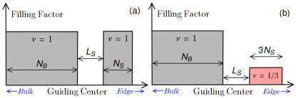
Figure 1: Schematic representation of two possible configurations at the reconstructed edge of the $\nu=1$ state. Letting the confining potential become smoother, $N_{S}$ electrons may separate from the bulk by $L_{S}$ guiding centers, forming a strip of (a) a $\nu=1$ state Chamon and Wen (1994) or (b) a $\nu=\frac{1}{3}$ Laughlin state.

The intricate edge structure involving a downstream $e^{*}=1$ mode along with a pair of counterpropagating $e^{*}=1/3$ modes has several experimental consequences. First, with such an edge structure the two-terminal (electrical) conductance would vary from $g_{\text{2T}}=e^{2}/h$ in a long sample (with full edge equilibriation) to $g_{\text{2T}}=5/3\times e^{2}/h$ in a short sample (with no equilibration) Protopopov et al. (2017); Nosiglia et al. (2018). This would be a smoking gun signature of the edge structure proposed here. Second, in the presence of disorder-induced tunneling and intermode interactions, the counterpropagating modes $e^{*}=1$ and $1/3$ are renormalized to two effective modes of charge $e^{*}_{{\uparrow}}$ and $e^{*}_{{\downarrow}}$ Kane et al. (1994); Kane and Fisher (1995); Protopopov et al. (2017) (here, ${\uparrow}/{\downarrow}$ denote the upstream/downstream modes). When biased, the upstream mode can carry a heat flow, which, in the particularly interesting case of $e^{*}_{{\uparrow}}=0$ and $e^{*}_{{\downarrow}}=2/3$, may appear without an accompanying upstream charge flow. Such neutral modes have been observed in hole-conjugate QH states Venkatachalam et al. (2012); Bid et al. (2009, 2010); Gurman et al. (2012); Gross et al. (2012); Inoue et al. (2014). Bias of the neutral modes can cause stochastic noise in the charge modes through the generation of quasihole-quasiparticle pairs Bid et al. (2010); Cohen et al. (2019); Park et al. (2019); Spånslätt et al. (2020). Below we show that this could account for the aforementioned Fano factor 1 Bhattacharyya et al. (2019). Moreover, neutral modes may also lead to suppression of interference in Mach-Zehnder interferometers Goldstein and Gefen (2016), in line with existing experiments.

Basic setup. We consider a $\nu=1$ state on a disk. In the symmetric gauge, $e\vec{A}/\hbar=(-y/2\ell^{2},x/2\ell^{2})$, the wave function of single-particle states in the lowest Landau level are ${\phi_{m}}(\vec{r}\,)=\left(r/\ell\right)^{m}e^{-im\theta_{\text{r}}}e^{-\left(\frac{r}{2\ell}\right)^{2}}/\sqrt{2^{m+1}\pi m!\ell^{2}}$, where $(r,\theta_{\text{r}})$ are the polar components of $\vec{r}$ in the $x$-$y$ plane; ${\phi_{m}}$ is an angular momentum eigenfunction with eigenvalue $\hbar m$, centered at $r=\sqrt{2m}\ell$ where $\ell$ is the magnetic length. Assuming spin-polarized electrons and neglecting higher Landau levels, the Hamiltonian is $H=H_{ee}+H_{c}$, where $H_{ee}$ is the interaction part while $H_{c}$ is a circularly symmetric one-body confining potential. Denoting $E_{c}=e^{2}/\epsilon_{0}\ell$, $H_{ee}=(E_{c}/2)\sum_{m_{1},m_{2},n}V_{m_{1}m_{2};n}^{ee}c_{m_{1}+n}^{\dagger}c_{m_{2}}^{\dagger}c_{m_{2}+n}c_{m_{1}}$ and $H_{c}=E_{c}\sum_{m}V_{m}^{c}c_{m}^{\dagger}c_{m}$, where $V^{ee}$ is the two-body Coulomb matrix element and $V^{c}$ is the matrix element of the confining potential. The total angular momentum $L$ is a good quantum number. The edge confining potential reads Meir (1994)

$$V_{c}(r)=\Bigg{\{}\begin{array}[]{cc}0&r<r_{0}-\frac{w\ell}{2},\\ \frac{s}{w\ell}\big{(}r-r_{0}+\frac{w\ell}{2}\big{)}&r_{0}-\frac{w\ell}{2}<r<r_{0}+\frac{w\ell}{2},\\ s&r>r_{0}+\frac{w\ell}{2},\end{array}$$ (4)

where $r_{0}$ is the radius of a compact $\nu=1$ state. The dimensionless parameter $s$ sets the overall height of the potential, which we henceforth fix to $s=7$. The steepness of the potential is controlled by the dimensionless width $w$.

We consider two classes of variational states (shown in Fig. 1), corresponding to an integer [Chamon-Wen Chamon and Wen (1994), Fig. 1(a)] and a fractional [Fig. 1(b)] reconstructed edge. Both are controlled by two parameters: the total occupancy $N_{S}$ of the reconstructed edge strip, and the number $L_{S}$ of empty orbitals separating it from the bulk. The latter contains $N_{B}$ electrons, such that the total number of electrons $N_{S}+N_{B}$ is fixed (to be 100). The Chamon-Wen family of states includes the compact edge configuration ($N_{S}=0=L_{S}$) which is the ground state for sharp confining potentials. For smoother confining potentials, the lowest energy state is expected to be at nonzero $N_{S}$ and $L_{S}$. In this case, a comparison of the energies of the states in the two classes determines whether fractionally charged modes could appear at the edge of the $\nu=1$ phase.

Variational ansatz: Integer edges.— Figure 1(a) represents a Slater-determinant state of $N_{S}+N_{B}$ electrons. It can be written as $|N_{B},0\rangle\otimes|N_{S},N_{B}+L_{S}\rangle$, where

$$|N,L\rangle=c_{L+N-1}^{\dagger}\,c_{L+N-2}^{\dagger}\,\ldots\,c_{L+1}^{\dagger}\,c_{L}^{\dagger}|0\rangle.$$ (5)

The energy and angular momentum of each state in the integer class of reconstructions can be found easily once the Coulomb matrix elements are known Sup .

Variational ansatz: Fractional edges. Figure 1(b) represents the product state of a Slater determinant ($|N_{B},0\rangle$) with an annulus of the $\nu=1/3$ Laughlin state, containing $N_{S}$ electrons starting at the guiding center $m=N_{B}+L_{S}$. The (unnormalized) wave function corresponding to the annulus is

$$\prod_{i=1}^{N_{S}}\bigg{[}z_{i}^{N_{B}+L_{S}}\bigg{]}\bigg{[}\prod_{i<j}\big{(}z_{i}-z_{j}\big{)}^{3}\bigg{]}e^{-\frac{1}{4}\sum_{i}|z_{i}|^{2}},$$ (6)

where $z_{n}=x_{n}-iy_{n}$ is the coordinate of the $n$th particle. The energy and angular momentum of states in this class involve the Coulomb energy and average occupations of the Laughlin state [Eq. (6)]. We evaluate these using standard classical Monte Carlo techniques Sup .

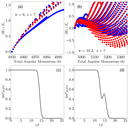
Figure 2: Variational analysis for $N_{S}+N_{B}=100$ and $s=7$. (a), (b) The energy of the two variational states as a function of the total angular momentum at (a) $w=6.0$ and (b) $w=10.2$. The energy of the unreconstructed state has been subtracted to make comparison easier. The blue (red) dots correspond to states with $\nu=1$ ($\nu=\frac{1}{3}$) reconstruction at the edge. For sharp edges ($w<10$) the ground state is the one with minimum angular momentum, implying that $L_{S}=0$, hence no edge reconstruction. In this case, we expect a single downstream edge mode supporting $e^{*}=1$ quasiparticles. For smooth edges ($w>10$) the ground state shifts to a higher angular momentum sector implying that the electronic disk expands and the edge undergoes reconstruction. (b) shows that a fractional reconstruction is energetically favorable to an integer reconstruction. This is true for all $w>10$. Thus the reconstructed edge supports counterpropagating modes with fractional charges. (c) and (d) depict the electronic densities of the ground state at (c) $w=6.0$ and (d) $w=10.2$. The nonmonotonic variation of density at the edge is another signature of the presence of additional emergent modes.

Results. Figure 2 shows the total energies and the ground state densities for the two class of variational states at different confining potentials. In Figs. 2(a) and 2(b) the blue dots correspond to integer edges while the red dots correspond to the fractional edge states. For a sharp confining potential [$w<10$, Fig. 2(a)] the lowest energy state is the one with the minimal angular momentum (in this case $4950\hbar$). This corresponds to the unreconstructed $\nu=1$ state with a single chiral edge mode. Figure 2(c) shows the electronic density in this case, which drops monotonically from $1/2\pi\ell^{2}$ to 0.

For smoother potentials [$w>10$, Fig. 2(b)] the lowest energy state has a much larger angular momentum ($5256\hbar$ for $w=10.2$ with $N_{S}=18$ and $L_{S}=0$) than the compact state. Correspondingly, Fig. 2(d) shows that the density varies nonmonotonically at the edge fno . The states with a fractional edge are found to have a lower energy than the states with an integer edge whenever reconstruction is favored Not . This is the main result of this work. We have verified that it does not depend on the precise form of the confining potential Sup . We now turn to discuss the experimental consequences of such a reconstruction and compare them to the observations reported in literature so far.

Figure 3: Two-terminal transport experiment at $\nu=1$, with an edge structure as calculated for a disk geometry (cf. text). The solid (dashed) lines indicate the integer (fractional) chirals at the two edges of the sample. The red (blue) chirals are biased (unbiased) due to the source S (drain D). For $L\ll\ell_{\text{eq}}$ ($\ell_{\text{eq}}$ is the intermode equilibriation length) the conductance is $g=5/3\times e^{2}/h$ ($3\times e^{2}/h$) for fractional (integer) edge reconstruction [cf. Figs. 1(b) and 1(a)]. For a fully equilibrated edge ($L\gg\ell_{\text{eq}}$), the conductance reduces to $g=e^{2}/h$ in both cases, as expected for the unreconstructed $\nu=1$ state.

Two-terminal conductance. Let us consider the setup shown in Fig. 3, where the edge structure is based on our analysis of a disk geometry. The chiral modes emanating from the source (S) are biased with respect to those emerging from the drain (D). Due to disorder-induced intermode tunneling, the counterpropagating chirals at each edge will equilibrate over a typical length $\ell_{\text{eq}}$. For a fully equilibrated edge ($L\gg\ell_{\text{eq}}$), the two-terminal conductance is $e^{2}/h$, as expected for the $\nu=1$ QH state. Note that this would be the case for both sharp and smooth edges and for both integer and fractional reconstructions.

For $L\ll\ell_{\text{eq}}$, the detailed structure of the edge underlies the conductance. For a sharp edge transport takes place through a single integer chiral, hence the electric conductance would retain the values $e^{2}/h$. This is different for smooth edges. The electric conductance is sensitive to the number as well as the nature of the modes; with a pair of counterpropagating fractional edges, the electric conductance becomes $5/3\times e^{2}/h$ Protopopov et al. (2017); Nosiglia et al. (2018). Such an observation would uniquely identify the edge structure proposed here [Fig. 1(b)]—a smoking gun signature of fractional edge reconstruction The .

Neutral modes. Consider the fractional reconstruction of Fig. 1(b). Labeling the outermost channel as $1$ and the innermost edge as $3$ [cf. Fig. 4(a)], the low energy dynamics of the three modes is described by three chiral bosonic fields $\phi_{j}$ ($j=1,2,3$) satisfying the Kac-Moody algebra, $[\phi_{j_{1}}(x),\phi_{j_{2}}(x^{\prime})]=i\pi\big{[}K^{-1}\big{]}_{j_{1},j_{2}}\text{sgn}(x-x^{\prime})$, where the $K$ matrix is diagonal with $K_{1,1}=3,K_{2,2}=-3,K_{3,3}=1$. The inner two modes are counterpropagating charge modes of $\nu=1$ and $\nu=1/3$ type. This is precisely the edge structure of the hole-conjugate $\nu=2/3$ FQH state. Since $L_{S}$ is typically small fno , in the presence of disorder-induced backscattering and interactions the two charge modes can hybridize [Fig. 4(a)], resulting in a downstream charged mode $\phi_{c}$ and an upstream neutral mode $\phi_{n}$, which are effectively decoupled at low energies Kane et al. (1994). This $K$ matrix is diagonal with $K_{1,1}=3,K_{c,c}=1,K_{n,n}=-1$. We note that here the outermost mode ($\phi_{1}$) is kept untouched (cf. Fig. 4).

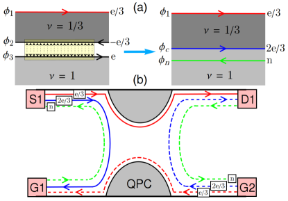
Figure 4: (a) Renormalization of the inner two edge modes due to interactions and disorder-induced backscattering into a downstream charge ($\phi_{c}$) and upstream neutral ($\phi_{n}$) mode. Only the inner two modes are assumed to couple, since within the variational calculation, the width of the $\nu=1/3$ strip increases as the edge potential is made smoother but the separation between the $\nu=1$ and $\nu=1/3$ regions remains constant. Thus the outermost edge mode ($\phi_{1}$) can be assumed to be physically separated from the inner two modes ($\phi_{2,3}$) Wang et al. (2013). (b) A single QPC tuned to the transmission plateau $t=1/3$. The bulk on both sides of the QPC is in the $\nu=1$ state with a reconstructed and renormalized edge. Solid (dashed) lines correspond to biased (unbiased) modes.

The experimental consequences of this emergent neutral mode are similar to the neutral modes in hole-conjugate states. For instance, it can lead to an upstream thermal current, which was reported in Ref. Venkatachalam et al. (2012), accompanied by an upstream shot noise (see below) Sabo et al. (2017); Spånslätt et al. (2019). The presence of the neutral mode can also hinder observation of interference effects in Mach-Zehnder setups Goldstein and Gefen (2016) as reported in Ref. Bhattacharyya et al. (2019).

Fractional conductance plateau and noise. The presence of fractionally charged chiral modes at the edge has clear experimental consequences for transport measurements. Consider for example the single QPC setup of Fig. 4(b). Here, the bulk filling factor is $\nu=1$ and the current is transmitted from the source (S1) to the drain (D1). When the QPC is fully open then the conductance would be $e^{2}/h$, as expected from the bulk topological index. However, due to the edge structure discussed above, it is also possible to pinch off the QPC, so that only the outermost mode ($\phi_{1}$) is transmitted while the inner two modes are completely reflected. In this case there would be a fractional conductance plateau at $1/3\times e^{2}/h$ while the bulk filling factor remains 1. Such a plateau was reported in Ref. Bhattacharyya et al. (2019).

Interestingly, although the conductance is quantized, the system could exhibit shot noise on the conductance plateau. Under the assumption of coherent propagation of the neutral mode, and provided certain symmetry conditions are satisfied Cohen et al. (2019); Park et al. (2020), the Fano factor is quantized. Such a quantized noise at the $1/3$ conductance plateau has been reported in Ref. Bhattacharyya et al. (2019). Below we sketch the underlying physics relying on our fractionally reconstructed edge picture.

Consider the setup shown in Fig. 4(b). The source S1 on the upper left-hand side of the QPC biases both charge modes emanating from it with the same voltage (say $V$). The current in the two modes is $I_{1}=V/3\times e^{2}/h$, $I_{c}=2V/3\times e^{2}/h$, and the total current is thus $I=I_{1}+I_{c}=V\times e^{2}/h$. The current ($I_{i}$, $i=1,c$) in a given mode is related to the corresponding quasiparticle density ($n_{i}$) through $I_{1}=e/3\times v_{1}n_{1}$ and $I_{c}=2e/3\times v_{c}n_{c}$, where $v_{i}$ are the corresponding velocities, implying $v_{1}n_{1}=v_{c}n_{c}$. Therefore if $N$ quasiparticles of charge $\frac{1}{3}$ emanate from the S1 in time $\tau$, then $N$ quasiparticles of charge $\frac{2}{3}$ also emanate in the same time interval. The total current ($I$) is $I=e/3\times N/\tau+2e/3\times N/\tau=eN/\tau$.

Now, on the upper right-hand side of the QPC, the outermost $e/3$ mode is biased while the inner $2e/3$ mode is grounded, and therefore the two modes will equilibrate through tunneling processes, which would also create excitations in the neutral mode. If there were $N$ quasiparticles in $\phi_{1}$, then after equilibration with $\phi_{c}$ there would be $N/3$ quasiparticles left in both charged modes and $2N/3$ neutral excitations in the upstream neutral mode. These neutral excitations would move to the lower right-hand side of the QPC and decay into quasiparticle-quasihole pairs in the charge modes. This generates stochastic noise in the charged modes because each decay process can randomly generate either a quasiparticle (quasihole) in the outermost (inner) mode or vice versa. This decay process would lead to a stochastic tunneling of $N/3$ electronic excitations into $\phi_{c}$, which eventually reach the drain D1. Similarly, on the lower left-hand side of the QPC, a biased $2e/3$ mode flows in parallel to an unbiased $e/3$ mode. Their mutual equilibration would again generate $2N/3$ neutral excitations. These decay on the upper left-hand side of the QPC and generate $2N/3$ excitations in the $\phi_{1}$ mode entering the drain D1.

As a result of the above, the charge entering the drain in time $\tau$ is $Q=e/3\times N/3+2e/3\times N/3+e/3\times\sum_{i=1}^{2N/3}a_{i}+2e/3\times\sum_{i=1}^{N/3}b_{i}$, where $a_{i}$ and $b_{i}$ are random variables which take values $\pm 1$ with equal probability, and describe the noise generated in the modes due to the neutral excitation decay described above. This implies that the average current arriving at the drain is $I_{D}=\langle Q\rangle/\tau=eN/3=I/3$ (consistent with a transmission of $1/3$). The variance of the charge is $\delta Q^{2}=\langle Q^{2}\rangle-\langle Q\rangle^{2}=e^{2}/9\times\sum_{i=1}^{2N/3}a_{i}^{2}+4e^{2}/9\times\sum_{i=1}^{N/3}b_{i}^{2}=2Ne^{2}/9=2e/9\times I\tau$. The effective Fano factor is $F_{\text{eff}}=\delta Q^{2}/I\tau\times 1/et(1-t)$. Using $t=1/3$ we obtain $F_{\text{eff}}=1$, which coincides with the observation of Ref. Bhattacharyya et al. (2019).

Conclusions. We have studied edge reconstruction at the boundary of $\nu=1$ integer quantum Hall state. Previously reported Hartree-Fock calculations show that upon smoothening the confining potential a new strip of $\nu=1$ QH state is formed at the edge, introducing counterpropagating integer modes Chamon and Wen (1994). Going beyond the mean-field approximation, we have performed a variational calculation, where we have compared the above ansatz to a new one, in which the electronic strip forms a $\nu=1/3$ Laughlin state. We have found that such fractional reconstruction is always energetically favorable, implying that fractional modes can appear at the boundary of integer QH states. We have discussed the experimental consequences of such a fractionally reconstructed edge, which nicely square with previous measurements, and provide predictions for future experiments. Our finding sets the stage for a future detailed investigation of coherent as well as incoherent transport in designed geometries, implementing the idea of fractionally reconstructed edges.

Supplemental material for “Fractional Edge Reconstruction in Integer Quantum Hall Phases” Udit Khanna Moshe Goldstein Yuval Gefen

S1 I.       Integer Reconstruction

Fig. 1(a) represents a Slater determinant of $N_{S}+N_{B}$ electrons. For convenience, we write it as the product of two Slater determinants, $|N_{B},0\rangle\otimes|N_{S},N_{B}+L_{S}\rangle$ where

$$|N,L\rangle=c_{L+N-1}^{\dagger}\,c_{L+N-2}^{\dagger}\,\ldots\,c_{L+1}^{\dagger}\,c_{L}^{\dagger}|0\rangle.$$ (S1)

The total angular momentum (in units of $\hbar$) of $|N,L\rangle$ is $NL+N(N-1)/2$, and that of the combined state is just the sum of the angular momenta of its two components

$$N_{S}L_{S}+\frac{1}{2}(N_{B}+N_{S})(N_{B}+N_{S}-1).$$ (S2)

The second term above is the angular momentum of the compact state ($L_{S}=0$). Thus the unreconstructed state has the smallest possible angular momentum for a fixed number of electrons ($N_{S}+N_{B}$) in the lowest Landau level. We have used $N_{S}+N_{B}=100$, which corresponds to minimum angular momentum 4950 ($\hbar$).

The energy of $|N,L\rangle$ is $\langle N,L|H_{ee}|N,L\rangle+\langle N,L|H_{c}|N,L\rangle$ where,

$$\langle N,L|H_{ee}|N,L\rangle =E_{c}\sum_{\begin{subarray}{c}i,j=L\\ (i<j)\end{subarray}}^{N+L-1}\bigg{(}V_{ij;0}^{ee}-V_{ii;j-i}^{ee}\bigg{)},$$ (S3)

$$\langle N,L|H_{c}|N,L\rangle =E_{c}\sum_{i=L}^{N+L-1}V_{i}^{c}.$$ (S4)

The energy of the full state consists of the sum of the energies of its constituents, as well as their two-body interaction energy,

$$E_{c}\sum_{i=0}^{N_{B}-1}\sum_{j=N_{B}+L_{S}}^{N_{B}+L_{S}+N_{S}-1}\bigg{(}V_{ij;0}^{ee}-V_{ii;j-i}^{ee}\bigg{)}.$$ (S5)

Therefore, the energy and angular momentum of each state in the integer class of reconstructions can be computed easily once the matrix elements are known. In the disk geometry, the Coulomb matrix elements for lowest Landau level states can be found analytically Tsiper (2002); Jain (2007). The matrix elements of confining potentials are given by,

$$V_{m}^{c} =\int d^{2}r\,V_{c}(r)|\phi_{m}(\vec{r}\,)|^{2}$$ (S6)

We note that for sharp and moderately smooth confining potentials ($w\leq 14$) and in the absence of Landau level and spin mixing, the minimum energy state within this class of reconstructions is precisely the ground state in the self-consistent Hartree-Fock (HF) approximation.

S2 II.       Fractional Reconstruction

Fig. 1(b) represents the product state of a Slater determinant ($|N_{B},0\rangle$) with an annulus of the $\nu=1/3$ Laughlin state ($|\Psi_{\frac{1}{3}}\rangle$), containing $N_{S}$ electrons starting at the guiding center $m=N_{B}+L_{S}$. The (unnormalized) wavefunction corresponding to $|\Psi_{\frac{1}{3}}\rangle$ is,

$$\prod_{i=1}^{N_{S}}\bigg{[}z_{i}^{N_{B}+L_{S}}\bigg{]}\bigg{[}\prod_{i<j}\big{(}z_{i}-z_{j}\big{)}^{3}\bigg{]}e^{-\frac{1}{4}\sum_{i}|z_{i}|^{2}},$$ (S7)

where $z_{i}=(x_{i}-iy_{i})/\ell$ is the coordinate of the $i$th particle.

The angular momentum of the (standard) Laughlin state with $N_{S}$ particles is $\frac{3}{2}N_{S}(N_{S}-1)$. Adding $N_{B}+L_{S}$ holes in the center increases the angular momentum by $N_{S}(N_{B}+L_{S})$. Then the combined state has a total angular momentum $N_{S}(L_{S}+N_{S}-1)+\frac{1}{2}(N_{B}+N_{S})(N_{B}+N_{S}-1)$. Comparing this expression with that of the corresponding integer-edge state, we note that this is larger by $N_{S}(N_{S}-1)$. This indicates that the electronic density of the fractionally reconstructed state varies much more smoothly than the corresponding integer reconstructed state.

The energy of the combined state is the sum of the energy of the two components (the $\nu=1$ bulk and the $\nu=1/3$ annulus) and their mutual interaction energy. The energy of $|\Psi_{\frac{1}{3}}\rangle$ is $\big{[}\langle\Psi_{\frac{1}{3}}|H_{ee}|\Psi_{\frac{1}{3}}\rangle+\langle\Psi_{\frac{1}{3}}|H_{c}|\Psi_{\frac{1}{3}}\rangle\big{]}/\langle\Psi_{\frac{1}{3}}|\Psi_{\frac{1}{3}}\rangle$ where

$$\langle\Psi_{\frac{1}{3}}|\Psi_{\frac{1}{3}}\rangle =\int\prod_{i}d^{2}r_{i}\big{|}\Psi_{\frac{1}{3}}\big{|}^{2},$$ (S8)

$$\langle\Psi_{\frac{1}{3}}|H_{ee}|\Psi_{\frac{1}{3}}\rangle =\int\prod_{i}d^{2}r_{i}\big{|}\Psi_{\frac{1}{3}}\big{|}^{2}\bigg{[}\sum_{i<j}\frac{E_{c}\ell}{|\vec{r}_{i}-\vec{r}_{j}|}\bigg{]},$$ (S9)

$$\langle\Psi_{\frac{1}{3}}|H_{c}|\Psi_{\frac{1}{3}}\rangle =E_{c}\sum_{m}\langle\Psi_{\frac{1}{3}}|c_{m}^{\dagger}c_{m}|\Psi_{\frac{1}{3}}\rangle V_{m}^{c},$$ (S10)

and its interaction energy with the bulk $\nu=1$ state is

$$E_{c}\sum_{i=0}^{N_{B}-1}\sum_{j=N_{B}+L_{S}}^{N_{B}+L_{S}+3N_{S}-3}\frac{\langle\Psi_{\frac{1}{3}}|c_{j}^{\dagger}c_{j}|\Psi_{\frac{1}{3}}\rangle}{\langle\Psi_{\frac{1}{3}}|\Psi_{\frac{1}{3}}\rangle}\bigg{(}V_{ij;0}^{ee}-V_{ii;j-i}^{ee}\bigg{)}.$$ (S11)

These expressions involve the Coulomb energy and average occupations of the Laughlin states, which we evaluate using standard classical Monte-Carlo techniques Jain (2007); Meir (1994); Mitra and MacDonald (1993) briefly described below.

Coulomb Energy

The Coulomb energy of $|\Psi_{\frac{1}{3}}\rangle$ is

$$\frac{1}{\int\prod_{i}d^{2}r_{i}\big{|}\Psi_{\frac{1}{3}}\big{|}^{2}}\int\prod_{i}d^{2}r_{i}\big{|}\Psi_{\frac{1}{3}}\big{|}^{2}\bigg{[}\sum_{i<j}\frac{E_{c}\ell}{|\vec{r}_{i}-\vec{r}_{j}|}\bigg{]}.$$ (S12)

Since $|\Psi_{\frac{1}{3}}|^{2}$ is real and positive, it can be interpreted as a (unnormalized) classical probability distribution Laughlin (1983). Writing $|\Psi_{\frac{1}{3}}|^{2}$ as a Boltzmann distribution $e^{-\beta U}$, we can make this interpretation concrete by recognizing $U$ as the potential for a two-dimensional plasma of charged particles in presence of an impurity of charge $N_{B}+L_{S}$ at the origin. The Coulomb energy can then be computed using standard Metropolis sampling Metropolis et al. (1953).

Average Occupation

The average occupation of $m^{\text{th}}$ single-particle state in $|\Psi_{\frac{1}{3}}\rangle$ is

$$\langle c_{m}^{\dagger}c_{m} \rangle_{1/3}=\frac{\langle\Psi_{\frac{1}{3}}|c_{m}^{\dagger}c_{m}|\Psi_{\frac{1}{3}}\rangle}{\langle\Psi_{\frac{1}{3}}|\Psi_{\frac{1}{3}}\rangle}$$

$$=\int d^{2}r_{1}\,d^{2}r_{2}\,\rho_{\frac{1}{3}}(\vec{r}_{1},\vec{r}_{2})\phi_{m}^{*}(\vec{r}_{1}\,)\phi_{m}(\vec{r}_{2}),$$ (S13)

where $\rho_{\frac{1}{3}}$ is the one-particle density matrix of $|\Psi_{\frac{1}{3}}\rangle$,

$$\rho_{\frac{1}{3}}(\vec{r}_{a}, \vec{r}_{b})=\frac{N_{S}}{\int\prod_{i}d^{2}r_{i}\big{|}\Psi_{\frac{1}{3}}\big{|}^{2}}\times$$ (S14)

$$\int\prod_{i=2}^{N_{S}}d^{2}r_{i}\Psi_{\frac{1}{3}}(\vec{r}_{a},\vec{r}_{2},\cdots)\Psi_{\frac{1}{3}}^{*}(\vec{r}_{b},\vec{r}_{2},\cdots).$$

Computing $\rho_{\frac{1}{3}}$ for all $\vec{r}_{a}$ and $\vec{r}_{b}$ using the above expression is very costly. To simplify the calculation, we note that both $\phi_{m}$ and $\Psi_{\frac{1}{3}}$ are eigenstates of the angular-momentum operator. Therefore the one-particle density matrix also satisfies

$$\rho_{\frac{1}{3}}(\vec{r}_{a}, \vec{r}_{b})=\sum_{m}\langle c_{m}^{\dagger}c_{m}\rangle_{1/3}\phi_{m}(\vec{r}_{a})\phi_{m}^{*}(\vec{r}_{b}).$$ (S15)

In the special case of $\vec{r}_{b}=re^{i\theta_{r}}$ and $\vec{r}_{a}=re^{i\theta_{r}+i\theta}$, the above expression reduces to

$$\rho_{\frac{1}{3}}(\vec{r}_{b},\theta;\vec{r}_{b})=\sum_{m}\langle c_{m}^{\dagger}c_{m}\rangle_{1/3}|\phi_{m}(\vec{r}_{b})|^{2}e^{-im\theta}.$$ (S16)

Since $\langle c_{m}^{\dagger}c_{m}\rangle_{1/3}$ is non-zero over a contiguous, finite and known range of $m$ [namely from $m=N_{B}+L_{S}$ to $m=N_{B}+L_{S}+3(N_{S}-1)$], the summation over $m$ can be restricted to this range without any error. Then we may interpret the above relation as a discrete Fourier transform from $m$ to its conjugate $\theta$ Mitra and MacDonald (1993). Inverting the Fourier transform we get

$$\langle c_{m}^{\dagger}c_{m}\rangle_{1/3}|\phi_{m}(\vec{r}\,)|^{2} =\frac{1}{3(N_{S}-1)+1}\times$$ (S17)

$$\sum_{j=0}^{3(N_{S}-1)}e^{im\theta_{j}}\rho_{\frac{1}{3}}(\vec{r},\theta_{j};\vec{r}\,),$$

where $\theta_{j}=2\pi j/[3(N_{S}-1)+1]$. Note that Eq. (S17) is only true for $N_{B}+L_{S}\leq m\leq N_{B}+L_{S}+3(N_{S}-1)$. In principle Eq. (S17) is valid for any value of $r$, but in practice the statistical error is minimum when $r\sim\sqrt{2m}\ell$ Mitra and MacDonald (1993). Since for large $m$, $|\phi_{m}|^{2}$ is very sharply peaked at this value of $r$, in this work we evaluate the occupation by integrating Eq. (S17) over $\vec{r}$ to get,

$$\langle c_{m}^{\dagger}c_{m}\rangle_{1/3} =\frac{1}{3(N_{S}-1)+1}\sum_{j=0}^{3(N_{S}-1)}e^{im\theta_{j}}\rho_{j},$$ (S18)

$$\text{where }\rho_{j} =\int d^{2}r\,\rho_{\frac{1}{3}}(\vec{r},\theta_{j};\vec{r}\,).$$ (S19)

Note that $\theta_{j}$ is not being integrated over in the previous expression. Then the occupation at any $m$ (within the appropriate range) can be found after we evaluate $\rho_{j}$ for all $j=0,\cdots,3(N_{S}-1)$. Using Eq. (S14) we have,

$$\rho_{j}= \frac{N_{S}}{\int\prod_{i}d^{2}r_{i}\big{|}\Psi_{\frac{1}{3}}\big{|}^{2}}\times$$ (S20)

$$\int\prod_{i=1}^{N_{S}}d^{2}r_{i}\Psi_{\frac{1}{3}}(\vec{r}_{1}e^{i\theta_{j}},\vec{r}_{2},\cdots)\Psi_{\frac{1}{3}}^{*}(\vec{r}_{1},\vec{r}_{2},\cdots).$$

From the definition of $\Psi_{\frac{1}{3}}$ we obtain

$$\Psi_{\frac{1}{3}}(\vec{r}_{1}e^{i\theta_{j}},\vec{r}_{2},\cdots)=\Psi_{\frac{1}{3}}(\{\vec{r}_{i}\})\times\mathcal{Z}_{1}(\theta_{j};\{\vec{r}_{i}\}),$$ (S21)

$$\mathcal{Z}_{a}(\theta_{j};\{\vec{r}_{i}\})=e^{-i\theta_{j}(N_{B}+L_{S})}\prod_{j\neq a}\frac{\big{(}z_{a}e^{-i\theta_{j}}-z_{j}\big{)}^{3}}{\big{(}z_{a}-z_{j}\big{)}^{3}}.$$ (S22)

Therefore, $\rho_{j}$ can be expressed as

$$\frac{1}{\int\prod_{i}d^{2}r_{i}\big{|}\Psi_{\frac{1}{3}}\big{|}^{2}}\int\prod_{i}d^{2}r_{i}|\Psi_{\frac{1}{3}}|^{2}\sum_{a=1}^{N_{S}}\mathcal{Z}_{a}(\theta_{j};\{\vec{r}_{i}\}),$$ (S23)

where we have symmetrized $\mathcal{Z}$ over all particles to increase the rate of convergence. The above expression has the same form as Eq. (S12) and can therefore be evaluated through very similar Metropolis sampling.

Figure S1: Results of the variational analysis using $100$ electrons with a charge-neutral confining potential. The blue (red) dots show the total energy of the variational states with a $\nu=1$ integer ($\nu=\frac{1}{3}$ fractional) side-strip as a function of the total angular momentum for a (a) sharp ($d=\ell$) and (b) smooth ($d=1.5\ell$) confining potential. Each curve corresponds to states with the same separation between the bulk and side-strip ($L_{S}$) but with different number of electrons in the side-strip ($N_{S}$). The curves shown here correspond to $L_{S}$ varying from $0$ to $30$ guiding centers. The energy of the unreconstructed state has been subtracted to make comparison easier. (a) For sharp edges $(d<1.3\ell)$ the ground state is the one with minimum angular momentum, implying no edge reconstruction. (b) For smooth edges $(d>1.3\ell)$ the ground state shifts to a higher angular momentum sector, implying that the electronic disk expands and the edge undergoes reconstruction. The minimum energy state lies on the curve corresponding to $L_{S}=0$. Panel (b) shows that a fractional reconstruction is energetically favorable to an integer reconstruction.

S3 III.       Charge Neutral Confining Potential

In the main text, the edge confining potential is modelled as a ramp function which interpolates linearly between two constants. Since any fairly smooth edge potential can be linearized around the chemical potential, we do not expect the results of our variational analysis to be modified by using a different smooth potential.

In order to verify this claim and properly compare our results with existing literature, we have repeated our variational analysis with a commonly used charge-neutral edge potential Zhang and Yang (2013); Wan et al. (2002, 2003); Hu et al. (2008, 2009). Specifically, the confining potential is modelled as the electrostatic potential of a positively charged background disk separated by a distance $d$ from the electron gas along the direction of the magnetic field. Therefore the confining potential defined in Eq. (1) of the main text is replaced by

$$V_{c}(r)=\int_{0}^{R}dr^{\prime}\int_{0}^{2\pi}d\theta\frac{E_{c}\sigma}{\sqrt{d^{2}+r^{2}+{r^{\prime}}^{2}-2r^{\prime}r\cos\theta}}$$ (S24)

where, the density ($\sigma$) and the radius ($R$) of the background disk depend on the bulk filling factor $(\nu_{B})$ and number of electrons ($N_{S}+N_{S}$) respectively. Charge neutrality of the full system requires $\sigma=\nu_{B}/2\pi\ell^{2}$ and $R^{2}=2(N_{S}+N_{B})\ell^{2}$ (where $\ell$ is the magnetic length). The resulting edge potential is quite sharp at $d=0$, and becomes smoother as $d$ increases.

Fig. S1 shows the total energies for the two class of variational states with a total of 100 electrons when this charge neutral potential is employed. The blue (red) dots correspond to different states with an integer (fractional) side-strip at the edge. The curves correspond to states with the same separation between the bulk and side-strip ($L_{S}$) and different number of electrons in the side-strip ($N_{S}$). Clearly for a sharp confining potential [$d<1.3\ell$, Fig. S1(a)] the lowest energy state is the one with the minimal angular momentum (in this case $4950\hbar$), which corresponds to the unreconstructed $\nu=1$ state.

For smoother potentials [$d>1.3\ell$, Fig. S1(b)] the lowest energy state has a much larger angular momentum ($5292\hbar$ for $d=1.5\ell$ with $N_{S}=19$ and $L_{S}=0$) than the compact state implying that the edge has undergone reconstruction. The states with a fractional edge are found to have a lower energy than the states with an integer edge for sufficiently smooth potentials. Thus the central result of this work is unaffected by the specific choice of confining potential.

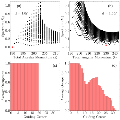
Figure S2: Results from exact diagonalization of the $\nu=1$ phase with 20 electrons restricted to 35 guiding centers. (a-b) The black dots shows the low energy spectrum as a function of the total angular momentum for a (a) sharp ($d=1.0\ell$) and (b) smooth ($d=1.35\ell$) confining potential (here $\ell$ is the magnetic length). The red dot corresponds to the exact ground state. The energy of the unreconstructed state has been subtracted to make comparison easier. (a) For sharp confining potentials, the ground state is in the lowest allowed angular momentum sector, implying no edge reconstruction. (b) For sufficiently smooth confining potentials, the ground state shifts to a larger angular momentum sector, implying the edge has undergone reconstruction. (c-d) depict the average occupation of the guiding centers in the exact ground state at (c) $d=1.0\ell$ and (d) $d=1.35\ell$. (d) shows that the filling factor at the reconstructed edge (and even its precise location) cannot be concluded from this analysis.

S4 IV.       Exact Diagonalization Analysis

In this section, we present an exact diagonalization (ED) analysis of the edge of $\nu=1$ phase. As described in the main text, we consider spinless electrons in the disk geometry and neglect higher Landau levels. Then the Hamiltonian is composed of a circularly symmetric one-body confining potential and the two-body Coulomb repulsion. Here we employ the charge-neutral confining potential described in Section III Zhang and Yang (2013); Wan et al. (2002, 2003); Hu et al. (2008, 2009). We include up to 20 electrons in 35 guiding centers ($m=0$ to $34$) and perform ED to find the low energy spectrum in several angular momentum sectors. Note that a relatively large number of electrons (as far as ED is concerned) is possible in our case because the bulk filling factor is 1. The average occupation of each guiding center is readily found from the ground state wavefunction.

Fig. S2 shows the spectrum and ground state occupations for $20$ electrons at two different confining potentials. In Figs. S2(a) and (b) the black dots show the low energy spectrum as a function of the total angular momentum while the red dot corresponds to the exact ground state. For a sharp confining potential [Fig. S2(a)] the ground state is the one with minimal angular momentum ($190\hbar$ for $20$ electrons). Fig. S2(c) shows that the average occupation of guiding centers in the ground state drops sharply from $1$ to $0$ at the edge. Clearly, this corresponds to the unreconstructed $\nu=1$ state.

For smoother confining potentials ($d>1.1\ell$, where $\ell$ is the magnetic length) the ground state shifts to a higher angular momentum sector indicating that the edge has undergone reconstruction. Fig. S2(b) shows that for $d=1.35\ell$, the ground state has angular momentum $230\hbar$ for which the average occupation of guiding centers [Fig. S2(d)] falls smoothly and non-monotonically from $1$ to $0$ at the edge. However, while the occupation of guiding centers close to the origin is $\sim 1$, the filling factor of the edge is far from quantized. Even the precise location of the edge is blurred. Both these issues arise due to the small number of electrons included in this analysis.

As is evident from this discussion, even 20 electrons are insufficient to make any conclusion regarding the precise filling factor of the side-strip formed at the edge during reconstruction or the nature of the emergent counter-propagating edge modes. This is a serious limitation of the ED method. Our variational analysis, on the other hand, allows us to address the problem of edge reconstruction within a quantum many-body framework using a very large number of electrons ($100$ in the current manuscript), and our results clearly indicate that fractional edge reconstruction is energetically favorable compared to integer reconstruction.

References

- Tsiper (2002) E. V. Tsiper, Analytic coulomb matrix elements in the lowest landau level in disk geometry, J. Math. Phys. 43, 1664 (2002).
- Jain (2007) J. K. Jain, Composite Fermions (Cambridge University Press, Cambridge, 2007).
- Meir (1994) Y. Meir, Composite edge states in the =2/3 fractional quantum hall regime, Phys. Rev. Lett. 72, 2624 (1994).
- Mitra and MacDonald (1993) S. Mitra and A. H. MacDonald, Angular-momentum-state occupation-number distribution function of the laughlin droplet, Phys. Rev. B 48, 2005 (1993).
- Laughlin (1983) R. B. Laughlin, Anomalous quantum hall effect: An incompressible quantum fluid with fractionally charged excitations, Phys. Rev. Lett. 50, 1395 (1983).
- Metropolis et al. (1953) N. Metropolis, A. W. Rosenbluth, M. N. Rosenbluth, A. H. Teller, and E. Teller, Equation of state calculations by fast computing machines, The Journal of Chemical Physics 21, 1087 (1953).
- Zhang and Yang (2013) Y. Zhang and K. Yang, Edge spin excitations and reconstructions of integer quantum hall liquids, Phys. Rev. B 87, 125140 (2013).
- Wan et al. (2002) X. Wan, K. Yang, and E. H. Rezayi, Reconstruction of fractional quantum hall edges, Phys. Rev. Lett. 88, 056802 (2002).
- Wan et al. (2003) X. Wan, E. H. Rezayi, and K. Yang, Edge reconstruction in the fractional quantum hall regime, Phys. Rev. B 68, 125307 (2003).
- Hu et al. (2008) Z.-X. Hu, H. Chen, K. Yang, E. H. Rezayi, and X. Wan, Ground state and edge excitations of a quantum hall liquid at filling factor 2/3, Phys. Rev. B 78, 235315 (2008).
- Hu et al. (2009) Z.-X. Hu, E. H. Rezayi, X. Wan, and K. Yang, Edge-mode velocities and thermal coherence of quantum hall interferometers, Phys. Rev. B 80, 235330 (2009).