Far-Infrared Photometric Redshifts: A New Approach to a Highly Uncertain Enterprise

Abstract

I present a new approach at deriving far-infrared photometric redshifts for galaxies based on their reprocessed emission from dust at rest-frame far-infrared through millimeter wavelengths. Far-infrared photometric redshifts (“FIR-$z$”) have been used over the past decade to derive redshift constraints for highly obscured galaxies that lack photometry at other wavelengths like the optical/near-infrared. Most literature FIR-$z$ fits are performed through $\chi^{2}$ minimization to a single galaxy’s far-infrared template spectral energy distribution (SED). The use of a single galaxy template, or modest set of templates, can lead to an artificially low uncertainty estimate on FIR-$z$’s because real galaxies display a wide range in intrinsic dust SEDs. I use the observed distribution of galaxy SEDs (for well-constrained samples across $0<z<5$) to motivate a new far-infrared through millimeter photometric redshift technique called MMpz. The MMpz algorithm asserts that galaxies are most likely drawn from the empirically observed relationship between rest-frame peak wavelength, $\lambda_{\rm peak}$, and total IR luminosity, L_IR; the derived photometric redshift accounts for the measurement uncertainties and intrinsic variation in SEDs at the inferred L_IR, as well as heating from the CMB at $z\lower 2.15277pt\hbox{$\;\buildrel>\over{\sim}\;$}5$. The MMpz algorithm has a precision of $\sigma_{\Delta z/(1+z)}\approx 0.3-0.4$, similar to single-template fits, while providing a more accurate estimate of the FIR-$z$ uncertainty with reduced chi-squared of order $\mathcal{O}(\chi^{2}_{\nu})=1$, compared to alternative far-infrared photometric redshift techniques (with $\mathcal{O}(\chi^{2}_{\nu})\approx 10-10^{3}$).

1 Introduction

Galaxies’ far-infrared spectral energy distributions are notoriously undersampled, whether or not the galaxies sit at $z=0$ or $z=7$. Data is sparse in this far-infrared through millimeter wavelength range (herein referred to as FIR/mm, at rest-frame $\sim$20$\mu$m–3 mm) because Earth’s atmosphere is largely opaque at these wavelengths; thus, we rely on insight from the limited far-infrared space-based missions (e.g. Spitzer, IRAS, ISO and the Herschel Space Observatory), or the limited view we can achieve through the handful of atmospheric windows we can peer through from the ground (e.g. with the James Clerk Maxwell Telescope, JCMT, the NOrthern Extended Millimeter Array, NOEMA, and the Atacama Large Millimeter and submillimeter Array, ALMA).

The FIR/mm wavelength regime is sensitive to reprocessed stellar emission, absorbed and re-radiated by dust in the interstellar medium (ISM), and is known to host a rich suite of spectral features useful for diagnostics of galaxies’ gas, metal and dust content. The most prominent characteristic of this regime is the superposition of modified blackbodies (of different temperatures and luminosities), originating from diffuse dust in the ISM. Most of the dust mass is relatively cold ($\approx$20-60 K), resulting in a peak of the SED around rest-frame $\lambda_{\rm peak}$ = 100$\pm$50$\mu$m. In the local Universe, there is a noted variation in SEDs’ luminosity-weighted dust temperature $T_{\rm d}$, a quantity that scales inversely with the observed rest-frame peak wavelength $\lambda_{\rm peak}$: from the $\sim$18 K dust in the Milky Way and similar L_⋆ galaxies to the $\sim$80 K dust in the dust-enshrouded Arp 220 or $\sim$60 K dust in the starburst galaxy M82. That same variance is seen at higher redshifts, with a general trend between $\lambda_{\rm peak}$ and L_IR, such that intrinsically more luminous galaxies are also hotter (e.g. Chapman et al., 2004; Casey, 2012; Kirkpatrick et al., 2012; Casey et al., 2018b). However, the relationship between $\lambda_{\rm peak}$ and L_IR has significant scatter, attributable to variable dust geometries.

Despite the measured variance in galaxies’ dust SEDs, it is common for 0^th order approximations for dust emission to take hold when there is little to no data available to analyze. For example, this is done especially when a source’s redshift is unconstrained and there is little to no other data (like a spectrum or photometric data in the radio/optical/near-infrared) available to constrain the redshift. In this case, the limited information available at FIR/mm wavelengths is used directly to place constraints on the redshift, a technique called far-infrared photometric redshift fitting (hereafter FIR-$z$ fitting). While this FIR-$z$ fitting technique is simple in its application, systematic offsets are especially problematic if the intrinsic dust SED of the fitted galaxy is significantly different than the template used to derive the FIR-$z$. FIR-$z$ fits also tend to have underestimated uncertainties due to a lack of accounting for the underlying variance in dust SEDs.

In this paper, I introduce a new approach at fitting far-infrared through millimeter photometric redshifts, using the empirical relationship between L_IR and $\lambda_{\rm peak}$, as well as photometric uncertainty. I call this fitting technique “MMpz,” shorthand for millimeter photometric redshift. The code is made available for public use including example use cases for well-known dusty star-forming galaxies. I compare this photometric redshift method with the use of single galaxy template FIR-$z$ fits, and related alternate FIR-$z$ techniques from the literature, with particular focus on their predicted uncertainties and accuracy. A brief history of FIR-$z$ fitting in the literature is given in § 2, while § 3 describes the MMpz approach to FIR-$z$ fitting. Quantitative tests of both techniques using mock and limited real data are described in § 4, and conclusions are described in § 5.

Figure 1: Example SEDs that are commonly used in the literature as representative of galaxies’ long wavelength SEDs, where the integral under the curve corresponds to the obscured star-formation rate via L_IR $\propto$ SFR. All SEDs are normalized to L_IR=$10^{12}$  L_⊙. Arp 220 is in red (Klaas et al., 1997; Rigopoulou et al., 1996), the Cosmic Eyelash in dot-dashed blue (Swinbank et al., 2010), the Pope et al. (2008) SMG composite in purple, the Swinbank et al. (2014) composite in gold, and a generic modified black body plus mid-infrared powerlaw that peaks at rest-frame $\lambda_{\rm peak}=100$$\mu$min dashed black. The right axis and light gray lines show the wavelengths of common FIR/mm continuum measurements and their corresponding rest-frame wavelengths at different redshifts.

2 Literature Techniques

Several works have used FIR photometric redshift fitting techniques to assess the redshifts of sources otherwise unconstrained through other data, dating back to the first observations of the first distant DSFGs in the late 1990’s. This section describes some of those methods broadly. Later in § 4, we compare between some of these techniques — in particular those that are not reliant on any photometric measurements outside of the FIR/mm regime (including radio wavelengths) — and the new approach outlined in § 3.

Some of the first studies recognizing the redshift evolution of submillimeter colors, thus the potential to use such measurements to constrain redshift, came in the very early days of bolometer observations at the JCMT. Hughes et al. (1997) modeled tracks of cold dust emission in 400$\mu$m/800$\mu$m color (then observed with the single-element bolometer UKT14) demonstrating strong redshift evolution beyond $z\sim 1$. Barger et al. (2000) combined the first 850$\mu$m datasets from Scuba with existing deep $\mu$Jy-radio imaging datasets from the VLA to derive a photometric redshifts based on an assumption of the FIR-radio correlation. Without detailed FIR SED constraints beyond the single 850$\mu$m Scuba point, they used an Arp 220 template (Klaas et al., 1997; Rigopoulou et al., 1996; Condon & Broderick, 1991) to tether the data, recognizing that such a template could be used to predict redshift from the 353 GHz-to-1.4 GHz flux density ratio. This technique relied on the assumption that the FIR-radio correlation (Helou et al., 1985) holds to high-redshift (c.f. Delhaize et al., 2017). The range of plausible redshifts for each source was then determined using a $\chi^{2}$ maximum likelihood technique. Aravena et al. (2010) use a similar FIR-radio-$z$ fitting method to for DSFGs discovered in the COSMOS field with unconstrained redshifts similarly focusing on the combination of the millimeter and radio continuum and use of Arp 220 as a prototypical template for the higher redshift DSFGs being fit.

Both of these approaches were practical given the available data at the time. In the 2000’s, DSFGs usually were only identified at one wavelength in the FIR/mm regime, and the use of radio counterpart identification was commonly used to astrometrically identify the most likely multiwavelength counterparts. The use of Arp 220 in these techniques was also sensible as it is a galaxy in the local Universe that sits in the same luminosity class of many of the analyzed high-$z$ DSFGs. The combination of a single FIR/mm photometric constraint with one radio photometric constraint can be an effective tool to constrain redshift due to the different $K$-corrections applied to either wavelength regime.

A more complex approach is outlined in Aretxaga et al. (2003), who use a set of 20 SEDs with different rest-frame peak wavelengths to generate a distribution in colors for galaxies as a function of redshift, drawn from an assumed integrated IR luminosity function (IRLF). The probability distribution in redshift for any given source of measured 850$\mu$m-to-1.4 GHz color (or 1.2 mm-to-1.4 GHz color) represents the set of mock galaxies at all redshifts (drawn at random from the sample of 20 templates) whose colors match that of the observed source. The galaxies used as templates are primarily in the local Universe, drawn from a mix of normal star-forming galaxies to ultraluminous infrared galaxies, plus a few $z\sim 2$ quasars with cold-dust emission. The breadth of SEDs in the Aretxaga et al. work leads to broader probability density distributions in redshift for any given source because of the degeneracy between dust temperature and redshift. This implies that the uncertainty on the FIR-$z$ fitting technique is naturally more realistic and representative of the true uncertainty of the redshift constraint in comparison to a single template fit.

In the analysis of bright Herschel sources, Ivison et al. (2016) tests the applicability of seven different template SEDs against those sources with confirmed CO-measured spectroscopic redshifts across the range $1.5<z<6$. These include four single-galaxy templates — SMM J2135-0102 at $z=2.3$ also known as the ‘Cosmic Eyelash’ (Swinbank et al., 2010), Arp 220 (Klaas et al., 1997; Rigopoulou et al., 1996), HFLS3 at $z=6.34$ (Riechers et al., 2013), and HATLAS J142413.9$+$022304, a lensed system at $z=4.2$ also known as G15.141 (Cox et al., 2011) — as well as three composite SEDs of different DSFG samples from Pope et al. (2008), Pearson et al. (2013) and Swinbank et al. (2014). Ivison et al. (2016) found that only three of these templates were good estimators of redshift: the Cosmic Eyelash, the Pope et al. (2008) composite SED and the Swinbank et al. (2014) composite SED. Of those three, the FIR-$z$ photometric redshift and its uncertainty is determined using a maximum likelihood estimator ($e^{-\chi^{2}}$) with the best-fit template.

Brisbin et al. (2017) present another FIR-$z$ method that does not rely on identification at 1.4 GHz explicitly, but is based solely on the FIR emission. They use a sample of 16 DSFGs with known spectroscopic redshifts, spanning $0.1<z<4.7$ with median $\langle z\rangle=2.2$. They us a simple inverted parabolic fit to the photometric data to infer the observed peak wavelength, $\lambda_{\rm observed\ peak}$. They then fit a linear relationship between redshift and $\lambda_{\rm observed\ peak}$ to anchor the FIR-$z$ model. The uncertainty in the FIR-$z$ fit is derived from the scatter in the linear relation between $z$ and $\lambda_{\rm observed\ peak}$.

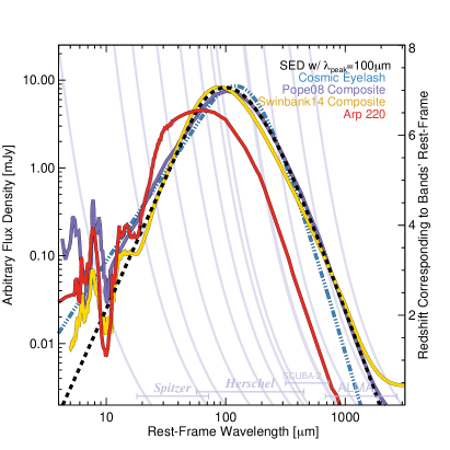
The template SEDs often used in the literature are shown in Figure 1 relative to a generic SED peaking at a rest-frame wavelength of $\lambda_{\rm peak}=100$ $\mu$m. In § 4, I draw comparisons between the literature approaches that are not anchored to any radio flux density measurements, primarily the single galaxy templates presented by Ivison et al. (2016) and the unique approach of Brisbin et al. (2017).

3 The “MMpz” Fitting Technique

3.1 Algorithm Design

The MMpz FIR-$z$ fitting technique is designed to provide an accurate estimate of a galaxy’s redshift based on its absolute FIR/mm photometry (rather than relative photometry alone) and an accurate representation of the uncertainty of that redshift estimate. A good representation of the uncertainty relies on an understanding of the intrinsic underlying variation of galaxies’ dust SEDs. Based on hundreds of Herschel-observed galaxies from $0<z<3$, and the South Pole Telescope sample of DSFGs observed toward higher redshifts (out to $z\sim 7$), Casey et al. (2018b) showed that galaxies’ dust SEDs follow a general trend relating the rest-frame peak wavelength $\lambda_{\rm peak}$ to the integrated IR luminosity L_IR via:

$$\langle\lambda_{\rm peak}(L_{\rm IR})\rangle=\lambda_{0}\bigg{(}\frac{L_{\rm IR}}{L_{t}}\bigg{)}^{\eta}$$ (1)

Where $\lambda_{0}$=102.8$\pm$0.4 $\mu$m, $L_{t}\equiv 10^{12}$  L_⊙, and $\eta=-0.068\pm 0.001$. This relation has a typical scatter in $\log($$\lambda_{\rm peak}$$)$ of $\sigma_{\log(\lambda)}=0.045$. This is given as Eq. 2 in Casey et al. (2018b). Physically, this relationship implies that more luminous galaxies have warmer luminosity-weighted dust temperatures, which may be driven by a combination of harder radiation fields from higher star formation rate densities and more compact dust geometries.

Figure 2: A visual illustration of the MMpz FIR-$z$ fitting technique using four spectroscopically-confirmed DSFGs at various redshifts: m450.173, a marginally-detected Scuba-2 450$\mu$m and 850$\mu$m source at $z=1.003$ (Casey et al., 2017), 850.20, a 850$\mu$m-detected Herschel-detected DSFG at $z=2.484$ (Casey et al., 2015), AzTEC-2, a 1.1 mm-selected DSFG at $z=4.63$ (AzTEC2; Jiménez-Andrade et al., 2020), and MAMBO-9, a 1-2 mm-selected DSFG confirmed at $z=5.85$ (Casey et al., 2019; Jin et al., 2019). The set of photometric constraints for each galaxy (shown at bottom) traces out a limited track in the L_IR-$\lambda_{\rm peak}$ plane, illustrated by the blue lines with associated uncertainty at each noted redshift represented by the thickness of the blue band. The uncertainty from the photometry in L_IR-$\lambda_{\rm peak}$ given the source’s photometry and spectroscopic redshift is shown in the purple 1$\sigma$ enclosed contour. The empirical relationship between L_IR and $\lambda_{\rm peak}$ is shown in the black line and associated 1$\sigma$ and 2$\sigma$ scatter, shown in gray and light gray. The probability density distribution in redshift is then constructed by sampling the gray shaded region (i.e. two dimensional probability distribution) along the blue redshift track (inset plots).

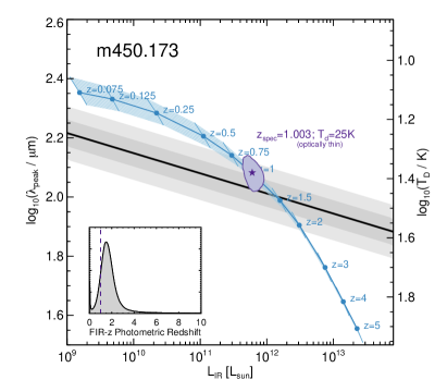
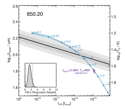
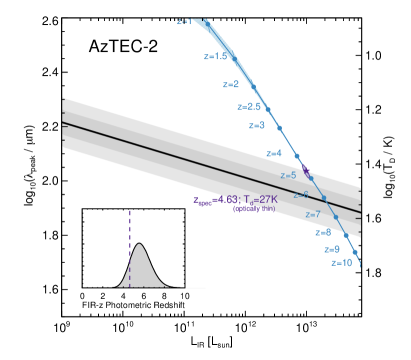
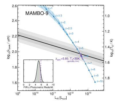
The luminosity dependence of the average peak wavelength is crucial information that MMpz folds into a galaxy’s FIR-$z$ fit. For example, a given set of FIR/mm photometry suggests a limited intrinsic range of IR luminosities, especially if that photometry is primarily on the Rayleigh-Jeans tail of the peak, where flux density (and thus L_IR) is roughly constant with redshift due to the very negative $K$-correction. Thus, FIR-$z$ fitting should make direct use of flux density measurements themselves, not just the contrast that is drawn between bands through FIR/mm colors. This is because sources with intrinsically brighter flux densities are more likely to have higher L_IR, and thus more likely to have intrinsically warmer dust SEDs. This strategy forms the backbone of the MMpz technique.

The algorithm is illustrated using a few examples of DSFGs with known redshifts in Figure 2: MAMBO-9 at $z=5.85$ (Casey et al., 2019), AzTEC-2 at $z=4.63$ (Jiménez-Andrade et al., 2020), 850.20 at $z=2.48$ (Casey et al., 2015), and m450.173 at $z=1.00$ (Casey et al., 2017). These systems are chosen because they span a wide redshift range and wide range of intrinsic SEDs. For all possible redshifts, the measured photometry constrain the range of possible SEDs in the L_IR and rest-frame $\lambda_{\rm peak}$ plane. Each galaxy traces out a track in the L_IR-$\lambda_{\rm peak}$ plane as a function of redshift. This track is shown in Figure 2 by the blue lines and shaded region of uncertainty reflective of photometric variance. The shape and direction of the blue curve traces the nature of the photometric constraints: an SED with measurements predominantly on the Rayleigh-Jeans tail translates to vertical tracks in this L_IR-$\lambda_{\rm peak}$ plane while photometry constraining the peak is more likely to result in uncertain L_IR and better constrained $\lambda_{\rm peak}$. This is perhaps counterintuative, because galaxies that are well sampled near their peaks should be relatively well constrained in both L_IR and $\lambda_{\rm peak}$; however, if the redshift is unknown, this introduces large uncertainty in L_IR because peak constraints do not benefit from the negative $K$-correction in the same fashion as do Rayleigh-Jeans constraints.

The thickness of this blue shaded region at each marked redshift traces out the $\pm$1$\sigma$ range of plausible SED solutions as measured using Markov Chain Monte Carlo (MCMC) modeling. We implement the MCMC fitting of the SED similarly to Casey et al. (2019), whereby the aggregate photometry is measured against SEDs with variable L_IR and $\lambda_{\rm peak}$ at a fixed redshift, and the likelihood of accepting a given SED in an MCMC chain is proportional to $e^{-\chi^{2}}$. Upper limits on photometric points are handled directly, whereby the algorithm takes as input both a flux density and uncertainty measurement, no matter the significance of the measurement; negative flux densities are also accepted as input (this can occur due to Gaussian fluctuations in a band with a non-detection).

Overall, the blue track in Figure 2 traces out the range of plausible L_IR and $\lambda_{\rm peak}$ values constrained by photometry across a range of redshifts. The gray region in Figure 2 centered on the black line traces out the empirical relationship and scatter (1$\sigma$ and 2$\sigma$) between $\lambda_{\rm peak}$ and L_IR from measured data as stated above in Equation 1; in other words, 95% of galaxies sit within the outer bounded light gray region, regardless of redshift.

The resulting MMpz probability density distribution in redshift (i.e. the FIR-$z$ fit) is then generated by sampling the empirical L_IR-$\lambda_{\rm peak}$ distribution (i.e. the two-dimensional gray distribution in Figure 2) along the redshift track traced out by the source’s photometry in L_IR-$\lambda_{\rm peak}$ (i.e. the blue tracks in Figure 2). In the absence of a direct crossing of a source’s redshift track and the mean L_IR-$\lambda_{\rm peak}$ relationship (i.e. the black line in Figure 2), the redshifts at which the two-dimensional probability distribution in L_IR-$\lambda_{\rm peak}$ is maximized along the redshit track are designated the most likely. The further the redshift track is from the peak of the distribution in L_IR-$\lambda_{\rm peak}$, the less well-constrained the FIR-$z$ fit will be.

In practice, the probability density distribution in redshift is constructed by (1) using a reference grid of SEDs populating the entire L_IR-$\lambda_{\rm peak}$ plane (described in the next subsection), (2) collapsing this grid of SEDs to the wavebands where observations have been collected for a given source; and then (3) comparing the grid model photometry to the source’s photometry using a $\chi^{2}$ maximum likelihood technique assuming Gaussian uncertainties in the data; in other words, each grid point in the L_IR-$\lambda_{\rm peak}$ plane has an associated $\chi^{2}$ with respect to the set of photometric constraints, and the likelihood is taken as $e^{-\chi^{2}}$ convolved with the probability density distribution of the given $\lambda_{\rm peak}$ as a function of L_IR. If a source has fewer photometric data points available, then the range of plausible SEDs in L_IR-$\lambda_{\rm peak}$ space will be broader than if there are many high quality photometric constraints. However, a well-constrained SED does not mean a well-constrained FIR-$z$ fit, due to the degeneracy of dust temperature and redshift with the observed peak wavelength, and relatively broad intrinsic range of SEDs even at a fixed L_IR.

3.2 Choice of SED shape and Input Information

The reference grid of SEDs used in MMpz is generated using a simple modified blackbody and mid-infrared powerlaw model as in Casey (2012), where $\alpha_{\rm MIR}=3$ represents the mid-infrared powerlaw slope and $\beta=1.8$ is the emissivity spectral index. Instead of using the analytic approximation as in Casey (2012), we use a piece-wise function for the modified blackbody plus mid-infrared powerlaw as in Casey et al. (2019).

What is the impact of these fixed values for $\alpha_{\rm MIR}$ and $\beta$ on the FIR-$z$ fit? A range of physical values for both parameters were tested for their impact on the output FIR-$z$ results. The probability density distribution in $z$ is completely insensitive to $\beta$ (given the negligible contribution of light on the Rayleigh-Jeans tail of the blackbody to L_IR). The mid-infrared $\alpha_{\rm MIR}$ slope has more impact. While real galaxies have a variety of mid-infrared powerlaw slopes, with lower values of $\alpha_{\rm MIR}\sim 1$ corresponding to more mid-infrared emission (perhaps hinting at hot dust surrounding an active galactic nucleus, AGN), the vast majority of DSFGs have moderately steep mid-infrared slopes, $2\lower 2.15277pt\hbox{$\;\buildrel>\over{\sim}\;$}\alpha_{\rm MIR}\lower 2.15277pt\hbox{$\;\buildrel>\over{\sim}\;$}5$. As $\alpha_{\rm MIR}$ increases, the mid-infrared component of the SED becomes negligible, contributing $\;\buildrel<\over{\sim}\;$5% to the total L_IR. Note that the DSFGs requiring a FIR-$z$ fit tend to have fewer rest-frame mid-infrared constraints than DSFGs that have alternate redshift estimators; the presence of mid-infrared counterparts implies that a optical/near-infrared counterpart is more likely to exist (Magdis et al., 2012), leading to an OIR constraint on the redshift. FIR-$z$ fits generated from data primarily on the Rayleigh-Jeans tail of blackbody emission are thus not impacted by the choice of $\alpha_{\rm MIR}$. In summary, we determine that our choice of $\alpha_{\rm MIR}=3$ and $\beta=1.8$ have minimal impact on the resulting FIR-$z$ fits from MMpz.

One important effect that the reference grid of SEDs takes into consideration is heating from the Cosmic Microwave Background at high-redshifts (at $z\lower 2.15277pt\hbox{$\;\buildrel>\over{\sim}\;$}5$; da Cunha et al., 2013). The CMB heats the ISM of high-$z$ galaxies, which in turn diminishes the contrast between the galaxy and its background, thus directly impacting the measured flux densities of dusty galaxies at sufficiently high redshifts (where the CMB temperature was much higher than it is today). The modeling of the impact of the CMB in the MMpz grid construction follows the prescription in da Cunha et al. (2013).

As input, the MMpz technique requires at least two flux density constraints in the FIR/mm. Non-detections can (and should) be included by reporting a measured flux density at a corresponding wavelength with associated flux density uncertainty. In practice, the list of photometric input datapoints can be an amalgamation of data from both single-dish telescopes and interferometers, including data with dramatically different beamsizes, sensitivities, etc. The user should make every attempt to reconstruct the intrinsic flux density of the given source from the given measured photometry, whether or not that includes accounting for a deboosting factor. Section 3.3 issues a cautionary note with respect to Herschel-SPIRE flux densities in particular, but the user should be aware that the MMpz algorithm itself will not directly account for any effects of confusion or Eddington boosting based on the instrument from which the data originates.

One subtle point to note is that the MMpz technique does not intrinsically account for the bandpass sensitivity curves of various FIR/mm instruments. Instead, it assumes reported flux densities are equal to the flux density intrinsic to the underlying SED. This is a common practice for fitting relatively simple SEDs to relatively sparse data at long wavelengths. This approximation greatly simplifies the computational burden of the algorithm, and is appropriate when the stated wavelength of observations is equal to the isophotal wavelength corresponding to the set of observations (e.g. as explicitly defined in Tokunaga & Vacca, 2005). In the FIR/mm, the differences between measuring flux densities as a convolution of a filter sensitivity curve and an underlying SED versus approximating flux density from the SED at a fixed wavelength amounts to a 1-3% effect, which is nearly always negligible relative to the total uncertainty in the flux density measurements.

Once a probability density distribution in redshift for a given source is in-hand, the optimum FIR photometric redshift FIR-$z$ is determined by taking the mode of the distribution and a 68% minimum credibility interval, or the minimum interval in redshift over which 68% of the distribution is contained. Adopting the mode of the distribution as the optimum redshift rather than the median redshift is appropriate in particular for bimodal or asymmetric probability distributions, which does occur fairly frequently using the MMpz technique.

3.3 A Cautionary note about Herschel-SPIRE

The Herschel Space Observatory SPIRE instrument has provided a wealth of data from 250–500$\mu$m across several extragalactic survey fields and over large swaths of the extragalactic sky (e.g. Oliver et al., 2012). This wavelength range can be crucial to constraining the peak of the SED for $z>1$ DSFGs. However, given the large beamsize of observations (18^′′–36^′′) and high on-sky source density, SPIRE maps are highly confused. The measured mean point-source confusion noise for SPIRE is 5.8, 6.3, and 6.8 mJy/beam at 250, 350, and 500$\mu$m, respectively (Nguyen et al., 2010); the confusion noise dominates over the instrumental noise in most SPIRE maps (with the exception being the shallowest SPIRE maps). Sophisticated deblending algorithms have attempted to use positional priors (e.g. from radio continuum, 24$\mu$m or other wavelengths where positions of sources are well-constrained) to extract and accurately measure flux densities below this confusion limit (Roseboom et al., 2010; Liu et al., 2018; Jin et al., 2018). While the technique of using positional priors is innovative and can be useful for characterizing populations of galaxies in aggregate, it is problematic when used to constrain the SED of an individual source that isn’t detected at high significance. In particular, these deblending algorithms are prone to under-estimating the uncertainty on a SPIRE flux density measurement dramatically, as they cannot account for uncharacterized uncertainty in the underlying model. Because the SPIRE data can have such a substantial impact on the shape of an SED fit despite this uncertainty, I caution users of the MMpz algorithm (and more broadly) to use the measured point-source confusion noise estimates as a lower limit on the flux density uncertainties for SPIRE.

4 Comparison between mmpz and other techniques

In this section I compare the MMpz FIR-$z$ technique to other radio-independent FIR-$z$ fitting techniques by generating SEDs of mock galaxies of known redshifts and use them to assess the accuracy and precision of each FIR-$z$ technique. In addition, a smaller sample of spectroscopically-confirmed real DSFGs is also used to compare methods as a check on the results generated from much larger samples of mock galaxies.

Figure 3: Redshift against $\Delta z/(1+z)$ for mock galaxies described in § 4. Values of $\Delta z/(1+z)>0$ indicate photometric redshifts higher than the mock galaxy’s true redshift, while values less than 0 are fit at lower redshifts. The solid tan region in each main panel shows excluded parameter space (i.e. corresponding to $z<0$, or blueshifted galaxies). Four panels represent single-template FIR-$z$ estimates: Arp220 (red, top left), the Cosmic Eyelash (blue, middle left), a 100$\mu$m-peaking SED (green, lower left), and the Pope et al. (2008) composite (purple, top right). The last two panels represent FIR-$z$ fits from the method outlined in Brisbin et al. (2017, yellow, middle right) and the MMpz technique (orange, bottom right). The right-most panel of each plot shows the collapsed, coadded probability density distributions in $\Delta z/(1+z)$ for the aggregate measurements of the mock galaxy population (solid colored histograms). The black hashed histogram denotes the predicted collapsed probability density distributions in $\Delta z/(1+z)$, if a mock galaxy’s estimated redshift is adopted as its true redshift. The single-template SED fits have much broader distributions in $\Delta z/(1+z)$ than would be predicted from the method’s reported uncertainties. The uncertainties in the Brisbin et al. (2017) method and the MMpz technique are well matched to the overall distribution in $\Delta z/(1+z)$, indicating both provide a better estimate of precision than single-template fits. Of these, the MMpz technique provides better overall accuracy.

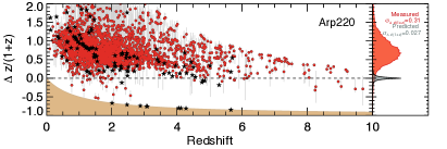
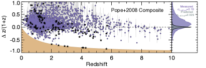
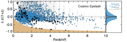
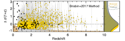
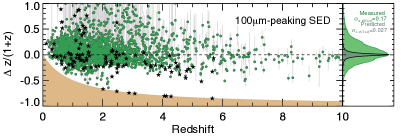
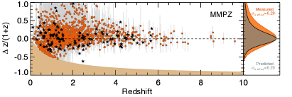
Mock galaxies are drawn from the observed distribution of galaxies in the L_IR-$\lambda_{\rm peak}$ plane following Equation 1 (with associated scatter), and following the best current estimate of the evolving IRLF as given in Zavala et al. (2018a). Thousands are simulated over a very large volume so that the technique can be tested over a wide range of redshifts and dynamic range in luminosity. Each mock galaxy is then downsampled in wavelength space to observing bands one might have on-hand for DSFGs in the literature, and Gaussian noise is added according to the typical RMS of observations in those bands with those instruments. These bands include Spitzer 24$\mu$m; Herschel-PACS 70$\mu$m, 100$\mu$m, and 160$\mu$m; Herschel-SPIRE 250$\mu$m, 350$\mu$m, and 500$\mu$m; Scuba-2 450$\mu$m and 850$\mu$m; AzTEC 1.1 mm; GISMO 2.0 mm; and ALMA bands 4–7 (from 870$\mu$m–2 mm). The typical uncertainties assumed for these bands are given in Table 1 of Casey et al. (2018b) and Table 1 of Casey et al. (2018a). It should be noted that many real galaxies will not have such a plethora of SED constraints as modeled here, particularly if they sit in regions of the sky not sampled by Herschel, or if fewer high-precision measurements exist from ALMA. Those galaxies will have more uncertain FIR-$z$ fits. The SED constraints that are modeled here are representative of constraints that are likely to exist for high-$z$ galaxies in extragalactic legacy fields (like COSMOS, UDS/CDF-S, SXDF, etc.). While our mock sample constrains many intrinsically faint systems, we require at least three photometric constraints above $>$3$\sigma$ significance for inclusion in our analysis, as galaxies falling below the detection thresholds will have no viable redshift constraints.

The spectroscopically-confirmed sample of DSFGs used to compare these FIR-$z$ fitting methods come from three parent samples: the Herschel-SPIRE selected sample of spectroscopically-confirmed DSFGs at $z\lower 2.15277pt\hbox{$\;\buildrel<\over{\sim}\;$}1.5$ from Casey et al. (2012), 13 ALESS 870$\mu$m-selected DSFGs from $1.5<z<2.5$ from Swinbank et al. (2014) and Danielson et al. (2017), 18 SCUBA-2 spectroscopically-confirmed DSFGs from $0.5\lower 2.15277pt\hbox{$\;\buildrel<\over{\sim}\;$}z\lower 2.15277pt\hbox{$\;\buildrel<\over{\sim}\;$}2.6$ from Casey et al. (2017) and the SPT-selected sample of lensed DSFGs from Weiß et al. (2013), with subsequent characteristics described in Strandet et al. (2016), Spilker et al. (2016) and Reuter et al. (2020). The Herschel sample is down-sampled to only include 62 galaxies detected at $>$4$\sigma$ in all three SPIRE bands, as galaxies with less than this have poorly constrained SEDs. The SPT sample photometry is corrected for gravitational lensing, as using uncorrected photometry would skew the results of the MMpz fits which depend on flux density as well as colors; 36 galaxies from the SPT sample have both well-measured magnification factors, $\mu$, and spectroscopic redshifts. In total, there are 129 galaxies in the spectroscopic sample spanning spectroscopic redshifts $0.1<z_{\rm spec}<5.7$.

Figure 4: Example mock galaxies’ SEDs (top panels) and their resulting FIR photometric redshift probability density distributions (bottom panels). The photometry from the intrinsic underlying SED is shown as black boxed points connected with a dotted line. Gaussian noise is added to each point according to the typical noise of observations in each band, and the photometric redshift fits are run on the noise-added photometry (gray circles). The overplotted gray SEDs represent draws from Markov Chain Monte Carlo trials fit to the mode of the MMpz redshift distribution, and the black solid SED is the median SED of those trials. The galaxies’ intrinsic properties and measured properties are quoted in the inset; the measured L_IR and $\lambda_{\rm peak}$ are quoted with fixed redshift. The bottom panels show the probability density distributions of various fitting methods (following the same color scheme as in Figure 3; no probability density function is given for the Brisbin et al. 2017 fits). Note that the $z\sim 2$ mock galaxy has a highly uncertain FIR-$z$ fit from MMpz due to the low signal-to-noise of many of the flux density constraints (and low L_IR).

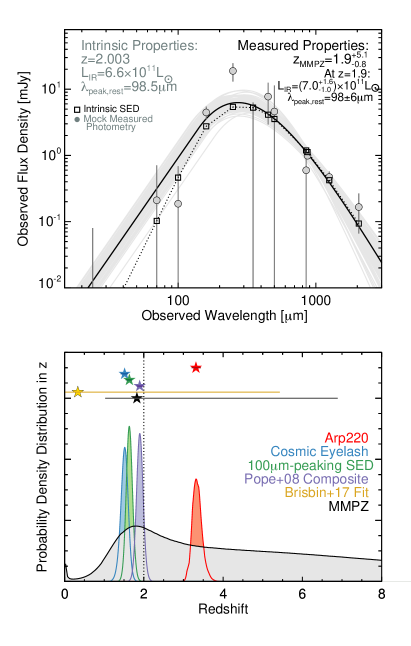
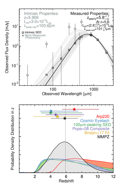
Figure 3 shows the accuracy and estimated precision of six FIR-$z$ techniques: four single SED fits (using an Arp220 template in red, the Cosmic Eyelash in blue, a 100$\mu$m-peaking SED in green, and the Pope et al. 2008 composite SED in purple), the Brisbin et al. (2017) technique in yellow and the MMpz technique in orange. The resulting FIR-$z$ fits for the spectroscopic sample are shown as black stars on each panel. Results from the 100$\mu$m-peaking SED are virtually identical to results using the Swinbank et al. (2014) composite SED so we only show one panel. The techniques that make use of a single-template SED vary in accuracy. The Arp220 SED, for example, seems to fit FIR-$z$ solutions skewed toward higher redshifts than the intrinsic simulated mock redshifts and spectroscopic redshifts. The Pope et al. (2008) composite spectrum also skews toward higher redshifts, whereas the Cosmic Eyelash and the 100$\mu$m-peaking SED fit fairly accurate SEDs for the overall distribution of galaxies. The primary shortcoming of these single-template fits, however, is the estimated precision in the FIR-$z$. The hashed gray distribution in each right histogram panel of Figure 3 highlights the distribution of uncertainties estimated using the given technique. A narrow distribution compared to the overall distribution of fits in $\Delta z/(1+z)$ (solid filled color histograms), represents a fit whose uncertainty has been dramatically under-estimated. This is the case for all single-template SED fits because they cannot account for the additional uncertainty brought on by a natural variance in galaxies’ SEDs.

In contrast to single-template fits, the Brisbin et al. (2017) and MMpz techniques have broad distributions for the predicted uncertainties. Because the predicted uncertainties are similarly broad to the overall distribution in $\Delta z/(1+z)$ for the entire population (i.e. the hashed gray and solid histograms in Figure 3 are similar), both the Brisbin et al. (2017) fits and the MMpz fits are far more likely to capture the precision to which constraints can be made from the FIR/mm photometry. Between the two fitting methods, the MMpz provides a much tighter and more accurate distribution in $\Delta z/(1+z)$.

Table 1: Summary of Goodness-of-Fit to FIR-$z$ Methods.

Method	Mock Galaxies					Real Spec-$z$ Confirmed Galaxies
	$\langle{\Delta z/(1+z)}\rangle$	$\sigma_{\Delta z/(1+z)}$	$\chi^{2}$	$\nu$	$\chi^{2}_{\nu}$	$\langle{\Delta z/(1+z)}\rangle$	$\sigma_{\Delta z/(1+z)}$	$\chi^{2}$	$\nu$	$\chi^{2}_{\nu}$
Arp220	0.71	0.31	$1.6\times 10^{6}$	2498	634	0.64	1.07	2.4$\times 10^{5}$	128	1860
Cosmic Eyelash	$-$0.02	0.19	$1.1\times 10^{5}$	2515	43.6	$-$0.02	0.43	5.9$\times 10^{4}$	128	459
100$\mu$m-peaking SED	0.04	0.17	$1.1\times 10^{5}$	2434	43.7	$-$0.06	0.64	6.1$\times 10^{4}$	128	475
Pope+08 Composite	0.14	0.19	$1.3\times 10^{5}$	2512	53.6	0.10	0.74	8.5$\times 10^{4}$	128	660
Brisbin+17	0.15	1.1	1100	1899	0.591	$-$0.03	4.63	22	97	0.24
MMpz	0.09	0.29	1600	1736	0.919	0.02	0.37	237	128	1.85

Table Notes: $\langle\Delta z/(1+z)\rangle$ captures the accuracy and $\sigma_{\Delta z/(1+z)}$ captures the precision of each fitting method. Negative values of $\langle\Delta z/(1+z)\rangle$ correspond to systematically lower FIR-$z$’s than truth, and positive values correspond to systematically higher FIR-$z$’s. Each mock galaxy test simulates 10⁴ galaxies, though only some fraction of those are above the detection thresholds in the simulated bands such that FIR-$z$’s can be fit. The number of mock/real galaxies simulated for each method is reflected in $\nu$, the degrees of freedom, whereby $\nu=n_{\rm mocks}-1$ or $\nu=n_{\rm real}-1$. The last column gives the reduced $\chi^{2}_{\nu}$; a value close to one represents appropriate precision on FIR-$z$ uncertainty. The spectroscopically-confirmed calibration sample of DSFGs shows the same trends as the mock galaxy sample though with a much smaller sample; the Brisbin et al. (2017) fit is unique in that many of the spectroscopically-confirmed galaxies had no valid photometric redshift due to lack of converged parabolic fit to photometry.

Note that both Ivison et al. (2016) and Zavala et al. (2018b) find a trend such that $\Delta z/(1+z)$ is systematically lower at higher redshifts than at lower redshifts. This ‘skew’ in FIR-$z$ fits is attributed to the adoption of a single-template SED technique, whereby the distribution of galaxies sampled have true variance in their SEDs. While this might be thought to be evidence of redshift evolution in galaxies’ average dust SEDs, the results from Figure 3 instead suggest that the effect is likely driven by the L_IR-$\lambda_{\rm peak}$ relation. The effect is especially strong for galaxies that are bright in the Herschel-SPIRE bands (as both those analyzed in Ivison et al. 2016 and Zavala et al. 2018b are). Galaxies of fixed Herschel flux densities will be intrinsically more luminous at higher redshifts, and at higher luminosities they are more likely to be intrinsically hotter according to the L_IR-$\lambda_{\rm peak}$ relation. If a single template SED is used, with fixed dust temperature, then at higher redshifts that template SED is likely cooler than the galaxies are intrinsically, thus the FIR-$z$ fit is more likely to peak at lower redshifts than reality. Such a trend is only seen in single-temperature SED fits (also visible in Figure 3), and it is not present in the Brisbin et al. (2017) fits or the MMpz fits.

Figure 4 shows two random mock galaxies taken from the distribution of simulated sources: one near $z\sim 2$ and another near $z\sim 6$. Their photometry vary in SNR from $\sim$10$\sigma$ to non-detections (whose 1$\sigma$ upper limits are shown) for the $z\sim 2$ mock system and from non-detections to $\sim$35$\sigma$ for the $z\sim 6$ mock system. The intrinsic SED is traced by square points and a dotted line, while the mock noise-added photometry, and resulting best-fit SEDs, shown in gray. The bottom panels of Figure 4 show the probability density distributions of each photometric redshift fitting technique analyzed for comparison with MMpz. In the case of the $z\sim 2$ source, we see a clear case of the single-template fits dramatically underestimating the uncertainties compared to the Brisbin et al. (2017) and MMpz estimates, while the $z\sim 6$ case sees a broader distribution in redshift for each technique, with the MMpz fit providing the most accurate estimate.

Table 1 summarizes the precision and accuracy of the fitting methods tested herein, both for the mock galaxies and for the spectroscopically-confirmed calibration sample of DSFGs. The $\langle\Delta z/(1+z)\rangle$ value gives the aggregate median of the distribution of $(z_{\rm FIR/mm}-z_{\rm real})/(1+z_{\rm real})$ for all sources and captures the fitting technique’s accuracy. The $\sigma_{\Delta z/(1+z)}$ parameter, which is the standard deviation in $\Delta z/(1+z)$, captures the breadth of the $\Delta z/(1+z)$ distribution for each fitting method, in other words, the precision of each fitting technique across large samples. The $\chi^{2}$ parameter is here defined as:

$$\chi^{2}=\sum_{i}\frac{(z_{\rm FIR/mm}-z_{\rm real})^{2}}{(\sigma_{\rm z_{\rm FIR/mm}})^{2}}$$ (2)

A reduced chi-squared statistic $\chi^{2}_{\nu}$ is quoted by dividing $\chi^{2}$ by the number of observations (in this case, independent mock or real galaxies) less the number of fitted parameters (in this case, only the redshift); thus, the degrees of freedom $\nu$ is equal to the number of mock or real galaxies analyzed minus one, ranging between $\approx$1700–2500 for the mocks.

Note that, assuming the fit is accurate, a reduced chi-squared, $\chi^{2}_{\nu}$, value far larger than one means that the uncertainties on the given measurement are under-estimated, while values significantly less than one imply an over-estimation of uncertainty. Our measurements show that single-template fits have reduced $\chi^{2}_{\nu}$ values significantly larger than one (of order $\mathcal{O}(\chi^{2}_{\nu})\approx$10¹–10³), reflective of the under-estimation of the uncertainties in the FIR-$z$. The Brisbin et al. (2017) method has $\chi^{2}_{\nu}=0.59$ for the mocks and $\chi^{2}_{\nu}=0.24$ for the spec-$z$ sample, suggesting an over-estimation of the uncertainties. The MMpz method has $\chi^{2}_{\nu}=0.92$ for the mocks and $\chi^{2}_{\nu}=1.85$ for the spec-$z$ sample. These values are the closest to one, suggesting the method’s uncertainties are accurately estimated. Of the two methods that produce $\chi^{2}_{\nu}\sim 1$ — the Brisbin et al. method and MMpz— the MMpz technique is more accurate ($\langle\Delta z/(1+z)\rangle<0.1$) and has better precision ($\sigma_{\Delta z/(1+z)}\approx 0.3-0.4$ vs. $\sigma_{\Delta z/(1+z)}\approx 1-5$).

5 Conclusions

The MMpz algorithm is introduced as a simple yet reliable technique for deriving a far-infrared/millimeter photometric redshift for distant galaxies. Code is made available to the community to fit a galaxy’s photometry and derive a probability density distribution in redshift based on the source’s photometry and the assumption that the galaxy will likely lie close to the average redshift-independent L_IR-$\lambda_{\rm peak}$ relationship. All available photometric constraints can be input, including non-detections.

The MMpz method contrasts to single galaxy template SED fits for redshifts because (1) it accounts for the broad distribution in intrinsic dust SEDs that galaxies are known to exhibit, and (2) it uses galaxies’ measured flux densities directly, and not just FIR/mm colors, to infer the most likely redshift solution. The first point ensures that the quoted precision of the FIR-$z$ measurement is not under-estimated, as is the case when a single-template SED is used. The second point addresses the observed trend in L_IR-$\lambda_{\rm peak}$. In other words, a galaxy with brighter intrinsic flux densities (but the same FIR/mm colors) is more likely to have a higher L_IR, and thus a shorter $\lambda_{\rm peak}$ (corresponding to an intrinsically hotter SED); an intrinsically hotter SED would mean that the source is more likely to sit at higher redshifts than a fainter galaxy with the same observed FIR/mm colors, though the uncertainty on both predicted redshift distributions would be broad.

Using samples of thousands of mock galaxies and 129 spectroscopically-confirmed DSFGs spanning a wide range of redshifts and intrinsic dust SEDs, I compare the MMpz technique to a variety of single-template SED FIR-$z$ fits in the literature, in addition to the technique outlined in Brisbin et al. (2017). As suspected, the single-template SEDs are found to dramatically under-estimate the uncertainties on FIR photometric redshifts. Both the Brisbin et al. (2017) and MMpz techniques do a good job of properly capturing the (low) precision of FIR-$z$ fits (with reduced chi-squared $\chi^{2}_{\nu}=0.6-0.9$), though the MMpz technique is found to have more accurate and precise ($\chi^{2}_{\nu}\approx 0.9-1.8$, $\langle\Delta z/(1+z)\rangle<0.1$, $\sigma_{\Delta z/(1+z)}\approx 0.3-0.4$) FIR-$z$ estimates across a wide redshift range.

The MMpz FIR-$z$ fitting technique is most useful for galaxies that lack constraints at wavelengths outside of the FIR/mm regime. For example, it may be of optimal use for large, wide-field surveys from single-dish millimeter telescopes (e.g. surveys from TolTEC on the LMT, or NIKA-2 on the IRAM-30 m) or alternatively, galaxies characterized with ALMA who fall outside of, or drop out from, deep optical/near-infrared imaging surveys. It should be emphasized that FIR-$z$ fitting in general is a “last resort” method of obtaining redshift constraints on distant galaxies, and it remains a highly uncertain enterprise. The core assumption at the root of the MMpz method is that galaxies fall on a redshift-invariant L_IR-$\lambda_{\rm peak}$ relationship within some statistical scatter; future measurements of large samples of dust SEDs for high-$z$ galaxies could reveal this core assumption to be invalid, but at present, existing measurements support this assumption out to $z\sim 6$. The intention behind the introduction of the MMpz algorithm is to provide a straightforward estimate of FIR/mm photometric redshifts that captures both the estimated redshift and its uncertainty as best as possible.

References

- Aravena et al. (2010) Aravena, M., Younger, J. D., Fazio, G. G., et al. 2010, ApJ, 719, 15
- Aretxaga et al. (2003) Aretxaga, I., Hughes, D. H., Chapin, E. L., et al. 2003, MNRAS, 342, 759
- Barger et al. (2000) Barger, A. J., Cowie, L. L., & Richards, E. A. 2000, AJ, 119, 2092
- Brisbin et al. (2017) Brisbin, D., Miettinen, O., Aravena, M., et al. 2017, ArXiv e-prints, arXiv:1708.05748
- Casey (2012) Casey, C. M. 2012, MNRAS, 425, 3094
- Casey et al. (2018a) Casey, C. M., Hodge, J., Zavala, J. A., et al. 2018a, ApJ, 862, 78
- Casey et al. (2012) Casey, C. M., Berta, S., Béthermin, M., et al. 2012, ApJ, 761, 140
- Casey et al. (2015) Casey, C. M., Cooray, A., Capak, P., et al. 2015, ApJ, 808, L33
- Casey et al. (2017) Casey, C. M., Cooray, A., Killi, M., et al. 2017, ApJ, 840, 101
- Casey et al. (2018b) Casey, C. M., Zavala, J. A., Spilker, J., et al. 2018b, ApJ, 862, 77
- Casey et al. (2019) Casey, C. M., Zavala, J. A., Aravena, M., et al. 2019, ApJ, 887, 55
- Chapman et al. (2004) Chapman, S. C., Smail, I., Blain, A. W., & Ivison, R. J. 2004, ApJ, 614, 671
- Condon & Broderick (1991) Condon, J. J., & Broderick, J. J. 1991, AJ, 102, 1663
- Cox et al. (2011) Cox, P., Krips, M., Neri, R., et al. 2011, ApJ, 740, 63
- da Cunha et al. (2013) da Cunha, E., Groves, B., Walter, F., et al. 2013, ApJ, 766, 13
- Danielson et al. (2017) Danielson, A. L. R., Swinbank, A. M., Smail, I., et al. 2017, ApJ, 840, 78
- Delhaize et al. (2017) Delhaize, J., Smolčić, V., Delvecchio, I., et al. 2017, A&A, 602, A4
- Helou et al. (1985) Helou, G., Soifer, B. T., & Rowan-Robinson, M. 1985, ApJ, 298, L7
- Hughes et al. (1997) Hughes, D. H., Dunlop, J. S., & Rawlings, S. 1997, MNRAS, 289, 766
- Ivison et al. (2016) Ivison, R. J., Lewis, A. J. R., Weiss, A., et al. 2016, ApJ, 832, 78
- Jiménez-Andrade et al. (2020) Jiménez-Andrade, E. F., Zavala, J. A., Magnelli, B., et al. 2020, arXiv e-prints, arXiv:2001.06997
- Jin et al. (2018) Jin, S., Daddi, E., Liu, D., et al. 2018, ApJ, 864, 56
- Jin et al. (2019) Jin, S., Daddi, E., Magdis, G. E., et al. 2019, arXiv e-prints, arXiv:1906.00040
- Kirkpatrick et al. (2012) Kirkpatrick, A., Pope, A., Alexander, D. M., et al. 2012, ApJ, 759, 139
- Klaas et al. (1997) Klaas, U., Haas, M., Heinrichsen, I., & Schulz, B. 1997, A&A, 325, 21
- Liu et al. (2018) Liu, D., Daddi, E., Dickinson, M., et al. 2018, ApJ, 853, 172
- Magdis et al. (2012) Magdis, G. E., Daddi, E., Sargent, M., et al. 2012, ApJ, 758, L9
- Nguyen et al. (2010) Nguyen, H. T., Schulz, B., Levenson, L., et al. 2010, A&A, 518, L5
- Oliver et al. (2012) Oliver, S. J., Bock, J., Altieri, B., et al. 2012, MNRAS, 424, 1614
- Pearson et al. (2013) Pearson, E. A., Eales, S., Dunne, L., et al. 2013, MNRAS, 435, 2753
- Pope et al. (2008) Pope, A., Chary, R., Alexander, D. M., et al. 2008, ApJ, 675, 1171
- Reuter et al. (2020) Reuter, C., Vieira, J. D., Spilker, J. S., et al. 2020, arXiv e-prints, arXiv:2006.14060
- Riechers et al. (2013) Riechers, D. A., Bradford, C. M., Clements, D. L., et al. 2013, Nature, 496, 329
- Rigopoulou et al. (1996) Rigopoulou, D., Lawrence, A., & Rowan-Robinson, M. 1996, MNRAS, 278, 1049
- Roseboom et al. (2010) Roseboom, I. G., Oliver, S. J., Kunz, M., et al. 2010, MNRAS, 409, 48
- Spilker et al. (2016) Spilker, J. S., Marrone, D. P., Aravena, M., et al. 2016, ApJ, 826, 112
- Strandet et al. (2016) Strandet, M. L., Weiss, A., Vieira, J. D., et al. 2016, ApJ, 822, 80
- Swinbank et al. (2010) Swinbank, A. M., Smail, I., Longmore, S., et al. 2010, Nature, 464, 733
- Swinbank et al. (2014) Swinbank, A. M., Simpson, J. M., Smail, I., et al. 2014, MNRAS, 438, 1267
- Tokunaga & Vacca (2005) Tokunaga, A. T., & Vacca, W. D. 2005, PASP, 117, 421
- Weiß et al. (2013) Weiß, A., De Breuck, C., Marrone, D. P., et al. 2013, ApJ, 767, 88
- Zavala et al. (2018a) Zavala, J. A., Montaña, A., Hughes, D. H., et al. 2018a, Nature Astronomy, 2, 56
- Zavala et al. (2018b) Zavala, J. A., Aretxaga, I., Dunlop, J. S., et al. 2018b, MNRAS, 475, 5585