Abstract

Motivated by the experimentally observed deviations from standard model predictions, we calculate the anomalous magnetic moments $a_{\alpha}=(g-2)_{\alpha}$ for $\alpha=e,\mu$ in a neutrino mass model originally proposed by Babu-Nandi-Tavartkiladze (BNT). We discuss two variants of the model, the original model plus a minimally extended version with an additional hypercharge zero triplet scalar. While the original BNT model can explain $a_{\mu}$, only the variant with the triplet scalar can explain both experimental anomalies. The heavy fermions of the model can be produced at the high-luminosity LHC and in the part of parameter space, where the model explains the experimental anomalies, it predicts certain specific decay patterns for the exotic fermions.

1 Introduction

Apart from neutrino masses, as observed in oscillation experiments [1, 2], there are only a few experimental hints for new physics. Among them is the long-standing deviation of the anomalous magnetic moment of the muon from the standard model (SM) prediction [5].

Currently, the experimental data gives a roughly 4$\sigma$ c.l. deviation [6, 7, 8, 9] from the standard model (SM) prediction:

$$\Delta a_{\mu}=(27.06\pm 7.26)\times 10^{-10}\,.$$ (1)

Two new experiments will shed light on this tension: E989 experiment at Fermilab [10] and E34 at J-PARC [11]. E989, running since 2018, and E34, planned to start in 2024, will improve the experimental accuracy by a factor 4 and 5, respectively, leading to a 5$\sigma$ c.l., in case the central value of the older measurement is confirmed.

From the theory side, there is still a debate about the SM calculation of the anomalous magnetic moment regarding hadronic vacuum polarization (HVP). A recent lattice-QCD result [12] for HVP bring the SM prediction of $(g-2)$ of the muon into agreement with experiments. However, this result is in tension with $e^{+}e^{-}\to$ hadrons cross-section data and global fits to electroweak precision observables [13].

More recently, a new precise measurement of the fine-structure constant [14] led to a deviation in the $(g-2)$ of the electron [15],

$$\Delta a_{e}=-(8.7\pm 3.6)\times 10^{-13}\,.$$ (2)

Although less significant (roughly 3$\sigma$ c.l.), it provides a new motivation to study $(g-2)$, as one might hope that both discrepancies have a common new physics origin. While both anomalies can be easily explained individually, the relative sign between $a_{\mu}$ and $a_{e}$ makes it more complicated to find a common explanation. Simple $Z^{\prime}$ (dark photon) models couple universally to electrons and muons, and cannot account for both discrepancies [16]. Several papers studying both anomalies in different contexts can be found in the literature [17, 18, 19, 20, 21, 22, 23, 24, 25, 26, 27, 28, 29, 30].

In this paper we study $(g-2)$ and the electric dipole moment (EDM) for the electron and muon in the context of the Babu-Nandi-Tavartkiladze (BNT) model [31] and a simple extension of it. The BNT neutrino mass model adds to the SM particle content vector-like fermion pairs $\left(\Psi,\overline{\Psi}\right)$, which transform as $SU(2)_{L}$ triplets, and a scalar quadruplet $S$. With these fields neutrino masses are induced at tree-level by a dimension 7 operator via the diagram shown in figure 1. By closing a pair of external scalar lines, a dimension 5 operator can also be generated with a loop.

Figure 1: Dimension 7 diagram responsible for neutrino masses in the BNT model.

However, with this particle content the Wilson coefficient $c_{R}^{\alpha\beta}$ of the electromagnetic (effective) dipole moment operator, i.e.

$$c_{R}^{\alpha\beta}\overline{\ell_{\alpha}}\sigma_{\mu\nu}P_{R}\ell_{\beta}F^{\mu\nu}+\textrm{h.c.}\,,$$ (3)

is suppressed by the small charged SM lepton masses, as can be seen from the diagrams in figure 2. Therefore, this model struggles to explain the current experimentally measured value of $\left(g-2\right)_{\mu}$, which significantly differs from the Standard Model value. To do so very large values for Yukawa couplings are required, which are close to the edge of non-perturbativity, given current limits on the exotic fermion masses, see section 4.

Figure 2: Diagrams responsible for the electromagnetic dipole moment operator in the BNT model. Note that the photon line can be attached to the internal scalar or fermion line.

As can be seen in eq. (3), a chirality flip (mass-insertion) is needed to close the effective operator. While the particle content of the original BNT model requires a Higgs insertion on the SM lepton line, the situation changes with the addition of an extra (complex) scalar triplet $\phi$ with no hypercharge. A summary of the extra fields in this extended BNT model — henceforth referred to as $\textrm{BNT}\phi$ — can be found in table 1. With this field content, the main contribution to the electromagnetic dipole moment operator becomes proportional to the mass of the heavy fermions $\left(\Psi,\overline{\Psi}\right)$ rather than the muon mass, as shown in figure 3 (diagram in the electroweak basis).

	Spin	$\mathrm{SU(3)}_{c}$	$\mathrm{SU(2)}_{L}$	$\mathrm{U(1)}_{Y}$
$\Psi$	$\frac{1}{2}$	${\bf 1}$	${\bf 3}$	$1$
$\overline{\Psi}$	$\frac{1}{2}$	${\bf 1}$	${\bf 3}$	$-1$
$S$	0	${\bf 1}$	${\bf 4}$	$\frac{3}{2}$
$\phi$	0	${\bf 1}$	${\bf 3}$	$0$

Table 1: Quantum numbers of the new fields in the extended BNT model, namely $\textrm{BNT}\phi$. It contains the complex $\phi$ scalar which is not part of the original BNT model. The Weyl fermions $\Psi$ and $\overline{\Psi}$ are unrelated (the bar in $\overline{\Psi}$ is simply a reminder that it has the opposite quantum numbers of $\Psi$). One can have any number of generations of vector fermions $\left(\Psi,\overline{\Psi}\right)$, for simplicity we fix the number of copies to 3.

Figure 3: Main contribution to the electromagnetic dipole moment operator in the $\textrm{BNT}\phi$ model. Note that the photon line can be attached to any of the internal scalars or fermion line.

The rest of the paper is divided as follows. In section 2 we describe in detail the $\textrm{BNT}\phi$ model. We derive the neutrino masses and the relevant mixings for the calculation of the Wilson coefficient $c_{R}^{\alpha\beta}$, directly related to $(g-2)$, EDM and Br($\ell_{\beta}\rightarrow\ell_{\alpha}\gamma$). At the end of the section we derive an analytical approximation for $c_{R}^{\alpha\beta}$, to provide some insight into the parameter dependence of the different observables. In section 3 we give and analyse the main results for the BNT and BNT$\phi$ models to compare both. We show that while the BNT$\phi$ model can explain both anomalous magnetic moments fulfilling the experimental constraints, the BNT model can only account for $(g-2)_{\mu}$ with values for the Yukawas at the edge of perturbativity. In section 4 we study the phenomenology of both models at colliders for the parameter space where they explain neutrino masses and the anomalous magnetic moments. We finally close with a short discussion of our results. Only the most relevant pieces of the Lagrangian are given in the main text. The full Lagrangian can be found in the appendix.

2 Model setup

2.1 Lagrangian, masses and mixings

We start by establishing a notation for the $SU(2)_{L}$ components of each field. We will assume that the components of $L$ and $H$ are organized in vectors,

$$L=\left(\begin{array}[]{c}\nu\\ \ell^{-}\end{array}\right)\;\textrm{and}\;H=\left(\begin{array}[]{c}H^{+}\\ H^{0}\end{array}\right)\,,$$ (4)

while the triplets $\Psi$, $\overline{\Psi}$ and $\phi$ are matrices:

$$\Psi=\left(\begin{array}[]{cc}\frac{\Psi^{+}}{\sqrt{2}}&\Psi^{++}\\ \Psi^{0}&-\frac{\Psi^{+}}{\sqrt{2}}\end{array}\right)\,,\;\overline{\Psi}=\left(\begin{array}[]{cc}\frac{\overline{\Psi}^{-}}{\sqrt{2}}&\overline{\Psi}^{0}\\ \overline{\Psi}^{--}&-\frac{\overline{\Psi}^{-}}{\sqrt{2}}\end{array}\right)\;\textrm{and}\;\phi=\left(\begin{array}[]{cc}\frac{\phi^{0}}{\sqrt{2}}&\phi^{+}\\ \phi^{-}&-\frac{\phi^{0}}{\sqrt{2}}\end{array}\right)\,.$$ (5)

Lastly, $S$ is is taken to be a 3-index symmetric tensor with the following components: $S_{111}=S^{+++}$, $S_{112}=S_{121}=S_{211}=S^{++}/\sqrt{3}$, $S_{122}=S_{212}=S_{221}=S^{+}/\sqrt{3}$ and $S_{222}=S^{0}$. The neutral scalars have non-zero vacuum expectation values (VEVs) which we will denote as $\left\langle H^{0}\right\rangle\equiv v_{H}/\sqrt{2}$, $\left\langle\phi^{0}\right\rangle\equiv v_{\phi}/\sqrt{2}$ and $\left\langle S^{0}\right\rangle\equiv v_{S}/\sqrt{2}$. The electroweak bosons acquire masses $m_{W}^{2}=g^{2}\left(v_{H}^{2}+4v_{\phi}^{2}+3v_{S}^{2}\right)/4$ and $m_{Z}^{2}=\left(g^{2}+g^{\prime 2}\right)\left(v_{H}^{2}+9v_{S}^{2}\right)/4$, therefore at tree-level the $\rho$ parameter has the value $\left(v_{H}^{2}+4v_{\phi}^{2}+3v_{S}^{2}\right)/\left(v_{H}^{2}+9v_{S}^{2}\right)$. In order for this number not to be far from unity, it follows that $v_{S}$ and $v_{\phi}$ need to be much smaller than $v_{H}$. Indeed, assuming that only one of these two VEVs is different from zero and using data from reference [8], the 3$\sigma$ upper limits for $\left|v_{\phi}\right|$ and $\left|v_{S}\right|$ are roughly 4 GeV and 2 GeV, respectively.

On top of the Standard Model couplings, the $\textrm{BNT}\phi$ model contains the following mass and interaction terms:

$$\mathcal{L}_{{\rm BNT}\phi} =M_{\Psi}\Psi\overline{\Psi}+Y_{\Psi}L\Psi H^{*}+Y_{\overline{\Psi}}\overline{\Psi}LS+Y_{e\phi}e^{c}\overline{\Psi}\phi+Y_{e\phi^{c}}e^{c}\overline{\Psi}\phi^{*}$$

$$+Y_{\Psi\phi}\Psi\overline{\Psi}\phi+Y_{\Psi\phi^{c}}\Psi\overline{\Psi}\phi^{*}-\mathcal{V}\,.$$ (6)

$$\mathcal{V} =m_{S}^{2}S^{*}S+m_{\phi}^{2}\phi^{*}\phi+\left(\mu_{\phi}^{2}\phi\phi+\mu_{H\phi}H^{*}H\phi+\lambda_{5}S^{*}HHH\right.$$

$$+\left.\lambda_{9}H^{*}H\phi\phi+\textrm{h.c.}\right)+\lambda_{6a}\left(H^{*}H\phi^{*}\phi\right)+\lambda_{6b}\left(H^{*}H\phi^{*}\phi\right)^{\prime}+\cdots\,.$$ (7)

We have omitted $SU(2)_{L}$ indices, as well as several scalar interactions which are of little importance for this work. Nevertheless, the full Lagrangian is displayed in appendix A. Flavour indices can be read from the equations above with the understanding that the coupling matrices have indices ordered according to the position of the fermions; for example $Y_{\Psi}L\Psi H^{*}=\left(Y_{\Psi}\right)_{ij}L_{i}\Psi_{j}H^{*}$.

From the requirement that the first derivative of the potential is null for the non-zero vacuum expectation values $v_{H}$, $v_{\phi}$ and $v_{S}$, together with the expected hierarchy of these VEVs, we get the approximate tadpole equations:

$$\mu^{2} \approx-\frac{\lambda_{1}v_{H}^{2}}{2}+2\left(m_{\phi}^{2}+2\mu_{\phi}^{2}\right)\frac{v_{\phi}^{2}}{v_{H}^{2}}\,,$$ (8)

$$\lambda_{5} \approx-2\frac{m_{S}^{2}}{v_{H}^{3}}v_{S}\,,$$ (9)

$$\mu_{H\phi} \approx 2v_{\phi}\frac{m_{\phi}^{2}+2\mu_{\phi}^{2}}{v_{H}^{2}}\,.$$ (10)

In the very first equation, $\mu^{2}$ and $\lambda_{1}$ are the SM scalar parameters: $\mathcal{V}_{SM}=\mu^{2}H^{*}H+\frac{1}{2}\lambda_{1}H^{*}H^{*}HH$. Note that $\mu_{H\phi}$ is a critical parameter for the electromagnetic dipole moment operator (see figure 3) which, through eq. (10), gets substituted by the VEV of $\phi^{0}$. On the other hand, $\lambda_{5}$ is fundamental for the generation of neutrino masses, as can be seen from diagram in figure 1, and its value is approximately proportional to the VEV of the $S^{0}$ scalar.

2.2 Neutrino masses

In the basis $\left(\nu,\Psi^{0},\overline{\Psi}^{0}\right)^{T}$ the full mass matrix for neutral fermions reads, at tree-level and in block form,

$${\cal M}^{0}=\begin{pmatrix}0&m_{Y_{\Psi}}&m_{Y_{\overline{\Psi}}}^{T}\\ m_{Y_{\Psi}}^{T}&0&M_{\Psi}\\ m_{Y_{\overline{\Psi}}}&M_{\Psi}^{T}&0\end{pmatrix},$$ (11)

where $m_{Y_{\Psi}}=Y_{\Psi}v_{H}/\sqrt{2}$ and $m_{Y_{\overline{\Psi}}}=Y_{\overline{\Psi}}v_{S}/\sqrt{2}$. With the standard seesaw approximation, if the entries in the matrices $m_{Y_{\Psi}}\left(M_{\Psi}^{-1}\right)^{T}$ and $m_{Y_{\overline{\Psi}}}\left(M_{\Psi}^{-1}\right)^{T}$ are smaller than 1, one can block-diagonalize ${\cal M}^{0}$ and the effective mass matrix for the light neutrinos is given by the expression

$$M_{\nu}=m_{Y_{\Psi}}\left(M_{\Psi}^{-1}\right)^{T}m_{Y_{\overline{\Psi}}}+m_{Y_{\overline{\Psi}}}^{T}M_{\Psi}^{-1}m_{Y_{\Psi}}^{T}\,.$$ (12)

Note that, without loss of generality, the $M_{\Psi}$ matrix can be taken to be diagonal.

If we take the neutrino mass diagram associated to this last formula (see figure 1) and close the outgoing Higgs $H^{*}$ line with one of the ingoing Higgses $H$, we obtain also a radiative contribution to neutrino masses already in the original BNT model. In the basis where $M_{\Psi}$ is diagonal, the correction to the tree-level formula can be expresses as

$$\Delta M_{\nu}^{{\rm Loop}}=\frac{1}{16\pi^{2}}\Big{(}m_{Y_{\Psi}}M_{{\rm Loop}}^{-1}m_{Y_{\overline{\Psi}}}+m_{Y_{\overline{\Psi}}}^{T}M_{{\rm Loop}}^{-1}m_{Y_{\Psi}}^{T}\Big{)}\,,$$ (13)

where $M_{{\rm Loop}}^{-1}$ is a diagonal matrix with entries

$$\left(M_{{\rm Loop}}^{-1}\right)_{ii}\approx\frac{m_{\Psi_{i}}}{m_{S}^{2}-m_{h}^{2}}\Delta B_{0}\left(m_{S}^{2},m_{h}^{2},m_{\Psi_{i}}^{2}\right)+\frac{m_{\Psi_{i}}}{m_{S}^{2}-m_{W}^{2}}\Delta B_{0}\left(m_{S}^{2},m_{W}^{2},m_{\Psi_{i}}^{2}\right)\,.$$ (14)

The quantity $\Delta B_{0}\left(m_{A}^{2},m_{B}^{2},m_{\Psi_{i}}^{2}\right)=B_{0}\left(0,m_{A}^{2},m_{\Psi_{i}}^{2}\right)-B_{0}\left(0,m_{B}^{2},m_{\Psi_{i}}^{2}\right)$ is related to the standard Passarino-Veltman function $B_{0}$. The main contribution to the radiative neutrino mass is shown in the left panel of figure 4. It should be noted that, with the introduction of the $\phi$ field, there is an extra loop contribution to neutrino masses (shown in the right panel of figure 4). Nevertheless, numerically its importance is small.

Figure 4: To the left: Dimension 5 diagram corresponding to the main one-loop neutrino mass contribution. To the right: Subleading dimension 7 neutrino mass contribution.

2.3 Scalar masses and mixing

In order to have a grasp on the magnitude and the parameter dependence of the electromagnetic dipole moment operator in expression (3), it is important to understand how do the various scalars mix. That discussion is simplified if we consider that the VEV of $S$ is negligible ($v_{S}\approx 0$), in which case this field does not mix with the remaining ones. All scalar components of $S$ can therefore be safely ignored (except in what concerns neutrino mass generation). However, we note that while this and other approximations made in the following discussion are very usefulness, to obtain the numerical results in section 3 we used the full un-approximated expressions for masses and mixing angles.

We are left with three scalars with electric charge +1 contributing for the dipole moment operator, namely $H^{+}$, $\phi^{+}$ and $\left(\phi^{-}\right)^{*}$. For this particular ordering of the fields, their mass-squared matrix is given by the approximate expression

$${\cal M}^{+} \approx\left(\begin{array}[]{ccc}2\frac{v_{\phi}^{2}}{v_{H}^{2}}\left(\kappa_{1}+\kappa_{2}\right)&\frac{\sqrt{2}v_{\phi}}{v_{H}}\kappa_{1}&\frac{\sqrt{2}v_{\phi}}{v_{H}}\kappa_{2}\\ \frac{\sqrt{2}v_{\phi}}{v_{H}}\kappa_{1}&\kappa_{3}&\kappa_{1}-\kappa_{3}\\ \frac{\sqrt{2}v_{\phi}}{v_{H}}\kappa_{2}&\kappa_{1}-\kappa_{3}&-\kappa_{1}+\kappa_{2}+\kappa_{3}\end{array}\right)\,,$$ (18)

with

$$\kappa_{1} \approx m_{\phi}^{2}+2\mu_{\phi}^{2}+\left(\lambda_{6a}+\lambda_{6b}+2\lambda_{9}\right)\frac{v_{H}^{2}}{2}\,,$$ (19)

$$\kappa_{2} \approx\kappa_{1}-\lambda_{6b}\frac{v_{H}^{2}}{2}\,,$$ (20)

$$\kappa_{3} \approx m_{\phi}^{2}+\left(\lambda_{6a}+\lambda_{6b}\right)\frac{v_{H}^{2}}{2}\,.$$ (21)

The properly normalized admixture of fields $v_{H}H^{+}-\sqrt{2}v_{\phi}\phi^{+}-\sqrt{2}v_{\phi}\left(\phi^{-}\right)^{*}$ constitutes the pseudo-Goldstone boson $G^{+}$, therefore we are left with only two other mass eigenstates: $\varphi_{1}^{+}$ and $\varphi_{2}^{+}$. In order to make a quantitative analysis of their masses and composition, we shall take into account that $v_{\phi}$ must be significantly smaller than $v_{H}$, which in turn is much smaller than the bare masses $m_{\phi}^{2}$ and $\mu_{\phi}^{2}$. When this is the case,

$$m^{2}\left(\varphi_{1}^{+}\right) \approx m_{\phi}^{2}+2\mu_{\phi}^{2}+\left(\lambda_{6a}+\frac{1}{2}\lambda_{6b}+2\lambda_{9}\right)\frac{v_{H}^{2}}{2}\,,$$ (22)

$$m^{2}\left(\varphi_{2}^{+}\right) \approx m_{\phi}^{2}-2\mu_{\phi}^{2}+\left(\lambda_{6a}+\frac{1}{2}\lambda_{6b}-2\lambda_{9}\right)\frac{v_{H}^{2}}{2}\,.$$ (23)

There is also the following relation between electroweak and mass eigenstates:

$$\left(\begin{array}[]{c}G^{+}\\ \varphi_{1}^{+}\\ \varphi_{2}^{+}\end{array}\right) \approx\left(\begin{array}[]{ccc}1&-\sqrt{2}\frac{v_{\phi}}{v_{H}}&-\sqrt{2}\frac{v_{\phi}}{v_{H}}\\ 2\frac{v_{\phi}}{v_{H}}&\frac{1}{\sqrt{2}}&\frac{1}{\sqrt{2}}\\ 0&-\frac{1}{\sqrt{2}}&\frac{1}{\sqrt{2}}\end{array}\right)\left(\begin{array}[]{c}H^{+}\\ \phi^{+}\\ \left(\phi^{-}\right)^{*}\end{array}\right)\,.$$ (33)

The neutral scalars, $H^{0}$ and $\phi^{0}$, are equally important in the loop diagrams 2. Splitting these two fields in their real and imaginary parts,

$$H^{0}\equiv\frac{H_{R}^{0}+iH_{I}^{0}}{\sqrt{2}}\,,\quad\phi^{0}\equiv\frac{\phi_{R}^{0}+i\phi_{I}^{0}}{\sqrt{2}},$$ (34)

it is easily seen that only the CP-even fields $H_{R}^{0}$ and $\phi_{R}^{0}$ mix to form two mass eigenstates. One of them should be identified with the observed 125 GeV Higgs boson and the other one we will call $R^{0}$. The CP-odd fields — $H_{I}^{0}$ and $\phi_{I}^{0}$ — do not mix, hence they are mass eigenstates. In particular, $H_{I}^{0}\equiv G^{0}$ is the neutral pseudo-Goldstone boson, just like in the Standard Model. The expressions for the mass eigenstates are

$$h^{0}\approx H_{R}^{0}+2\frac{v_{\phi}}{v_{H}}\phi_{R}^{0},\quad R^{0}\approx\phi_{R}^{0}-2\frac{v_{\phi}}{v_{H}}H_{R}^{0},\quad G^{0}=H_{I}^{0},\quad\phi_{I}^{0}\,,$$ (35)

with the corresponding (pseudo)masses given by the following formulas:

$$m^{2}\left(h^{0}\right)\approx 4\lambda_{1}v_{H}^{2}-4\left(m_{\phi}^{2}+2\mu_{\phi}^{2}\right)\frac{v_{\phi}^{2}}{v_{H}^{2}}\,,\quad m^{2}\left(R^{0}\right)\approx m^{2}\left(\varphi_{1}^{+}\right)\,,$$ (36)

$$m^{2}\left(G^{0}\right)=0\,,\quad m^{2}\left(\phi_{I}^{0}\right)\approx m^{2}\left(\varphi_{1}^{-}\right)\,.$$ (37)

2.4 Analytical understanding of the value of $\left(g-2\right)_{e,\mu}$ and related observables

With the approximate dependence of masses and mixing angles on the various Lagrangian parameters, we are in a position to estimate the value of $g-2$ for the electron and the muon, as well as the value of the lepton electric dipole moments and the branching ratios $\textrm{Br}\left(\ell_{\beta}\rightarrow\ell_{\alpha}\gamma\right)$. Nevertheless, for our numerical results we used the full one-loop expressions, without approximations.

Following [17], we can describe a generic interaction of a fermion $\Psi$ with the charged leptons $\ell_{\alpha}=e,\mu,\tau$ and a scalar $\Phi$ with couplings $\Gamma_{L}^{\alpha}$ and $\Gamma_{R}^{\alpha}$:

$$\mathscr{L}=\cdots+\overline{\Psi}\left(\Gamma_{L}^{\alpha}P_{L}+\Gamma_{R}^{\alpha}P_{R}\right)\ell_{\alpha}\Phi^{*}+\textrm{h.c.}$$ (38)

Through a loop diagram, this interaction will induce a contribution to the electromagnetic dipole moment operator shown in eq. (3). Specifically, reference [17] quotes the result

$$c_{R}^{\alpha\beta}\approx\frac{1}{16\pi^{2}}\Gamma_{L}^{\alpha*}\Gamma_{R}^{\beta}\frac{m_{\Psi}}{m_{\Phi}^{2}}\left[f_{\Phi}\left(\frac{m_{\Psi}^{2}}{m_{\Phi}^{2}}\right)+q_{\Psi}g_{\Phi}\left(\frac{m_{\Psi}^{2}}{m_{\Phi}^{2}}\right)\right]$$ (39)

plus sub-leading contributions which are suppressed by the masses of the leptons $\ell_{\alpha}$ and $\ell_{\beta}$. The loop functions appearing in this expression are

$$f\left(x\right) =\frac{x^{2}-1-2x\log x}{4\left(x-1\right)^{3}}\,,$$ (40)

$$g\left(x\right) =\frac{x-1-\log x}{2\left(x-1\right)^{2}}\,,$$ (41)

and $q_{\Psi}$ is the electric charge of the loop fermion, flowing from the initial lepton ($\ell_{\beta}$) to the final one ($\ell_{\alpha}$).

The lepton anomalous magnetic moments, their electric dipole moments, as well as the branching ratios of the decays $\ell_{\beta}\rightarrow\ell_{\alpha}\gamma$ can readily be calculated from the numbers $c_{R}^{\alpha\beta}$:

$$\frac{\left(g-2\right)_{\alpha}}{2}\equiv a_{\alpha} =-4\frac{m_{\ell_{\alpha}}}{e}\,\textrm{Re}\,c_{R}^{\alpha\alpha}\,,$$ (42)

$$d_{\alpha} =-2\,\textrm{Im}\,c_{R}^{\alpha\alpha}\,,$$ (43)

$$\textrm{Br}\left(\ell_{\beta}\rightarrow\ell_{\alpha}\gamma\right) =\frac{m_{\ell_{\beta}}^{3}}{4\pi\Gamma_{\ell_{\beta}}}\left(\left|c_{R}^{\alpha\beta}\right|^{2}+\left|c_{R}^{\beta\alpha}\right|^{2}\right)\,.$$ (44)

For the particular model under discussion, the main contribution to $c_{R}^{\alpha\beta}$ is due to the loop shown in figure 3. With the approximate value of the scalar mixing matrices provided earlier, we obtain the following estimate:

$$c_{R}^{\alpha\beta} \approx\frac{1}{16\pi^{2}}\sum_{i=1}^{3}\left(Y_{\Psi}\right)_{\alpha i}\left(Y_{e\phi}+Y_{e\phi^{c}}\right)_{\beta i}m_{\Psi_{i}}\frac{v_{\phi}}{v_{H}}$$

$$\times\sum_{\Phi=\left\{G^{+},h^{0},\varphi_{1}^{+},R^{0}\right\}}\frac{\kappa_{\Phi}}{m_{\Phi}^{2}}\left[f\left(\frac{m_{\Psi_{i}}^{2}}{m_{\Phi}^{2}}\right)-\kappa_{\Phi}^{\prime}g\left(\frac{m_{\Psi_{i}}^{2}}{m_{\Phi}^{2}}\right)\right]\,.$$ (45)

The $\kappa_{\Phi}^{(\prime)}$ coefficients in this expression take the following values: $\kappa_{G^{+},h^{0},\varphi_{1}^{+},R^{0}}=\left(-\sqrt{2},1,\sqrt{2},-1\right)$ and $\kappa_{G^{+},h^{0},\varphi_{1}^{+},R^{0}}^{\prime}=\left(2,1,2,1\right)$. At leading order, the remaining scalars do not contribute. Note also that the present model does not contain extra gauge bosons, however the couplings of the Standard Model ones to leptons is slightly altered. Instead of considering an extra loop with an internal $W^{\pm}$ boson, it is sufficient to include in the scalar computation the pseudo-Goldstone boson $G^{+}$, assigning to it its physical mass ($m_{G^{+}}=m_{W}$).

3 Results and discussion

In this section we will discuss the numerical results for $\Delta(g-2)_{\alpha}$ ($\alpha=e,\mu$), the neutrino mass fits and constraints from charged lepton flavour violation (cLFV) searches. We also briefly comment on electric dipole moments, $d_{e,\mu}$. The discussion is divided into two parts. In the first one, we show results for the original BNT model, while the second discusses the extended version, BNT$\phi$.

We have implemented the model into SARAH [32, 33]. This program generates SPheno routines [34, 35] for a numerical calculation of mass spectra and other observables. To cross-check the results, we have written private codes for numerical evaluation of $\Delta(g-2)_{\alpha}$ and implemented also the approximation formulas discussed in 2.

3.1 Results for the BNT model

Since the main motivation for the BNT model [31] is to explain the observed neutrino oscillation data, we first briefly discuss, how neutrino masses and angles can be fitted to the experimental data.

The master parametrization [36, 37] allows us to fit any Majorana neutrino mass model to experimental data. For the case of the BNT model, the general formulae in [37] simplify to

$$Y_{1}=cM_{\Psi}^{1/2}WT{\hat{m}_{\nu}}^{1/2}U_{\nu}^{\dagger}\,,$$ (46)

$$Y_{2}=cM_{\Psi}^{1/2}W^{*}B{\hat{m}_{\nu}}^{1/2}U_{\nu}^{\dagger}\,,$$

with

$$B=(T^{T})^{-1}(\mathbb{I}-K)\,,$$ (47)

and $c=(v_{H}v_{S})^{-1/2}$. Since the neutrino mass matrix is symmetric under the exchange of $Y_{1}$ and $Y_{2}$, we can associate $Y_{\Psi}$ and $Y_{\overline{\Psi}}$ with either of them arbitrarily. The master parametrization calculates the two Yukawa matrices as function of the input parameters, $m_{\nu_{i}}$, $U_{\nu}$ and $M_{\Psi}$ and three matrices, $W$, $T$ and $K$ with arbitrary parameters. Here, $W$ is a unitary, $T$ an upper triangular and $K$ an antisymmetric matrix. All matrices are $(3,3)$. As usual, ${\hat{m}_{\nu}}$ and $U_{\nu}$ are the light neutrino mass eigenvalues and mixing matrix.

Figure 5: Left: $\Delta(g-2)_{\alpha}$, the shift with respect to the standard model value of $(g-2)_{\alpha}$, as a function of $|(Y_{\Psi})_{11}|$ for 2 choices of the quadruplet VEV, $v_{S}$. Shown are only $\alpha=e,\mu$, since for the $\tau$ there is practically no experimental information. The thin horizontal bands are the 1 $\sigma$ c.l. ranges of the experimental anomalies. Right: Br$(l_{i}\to l_{j}\gamma$) for the same choice of parameters as the left figures. The masses of $\Psi_{i}$ are chosen with $m_{\Psi_{1,2,3}}=(0.8,0.9,1.0)$ TeV, the mass of the scalar quadruplet is $m_{S}=500$ GeV. For the neutrino fit, see the discussion in the text.

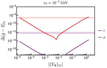
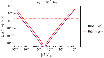
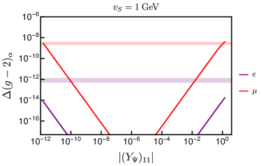
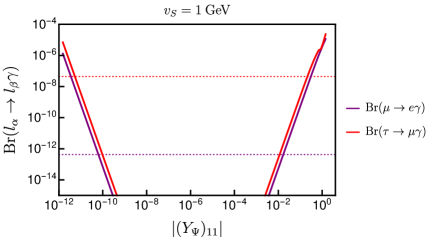
An especially simple case is the choice $W=\mathbb{I}$, $T=f\times\mathbb{I}$ and $K=0$. This leads to $Y_{\Psi}=f^{2}Y_{\overline{\Psi}}^{T}$ and both Yukawa matrices are equal for $f=1$. With this choice, both Yukawa matrices have off-diagonal elements, due to the large mixing angles, observed in oscillation experiments. Fig.(5) shows $\Delta(g-2)_{\alpha}$ and Br$(l_{i}\to l_{j}\gamma)$ for some fixed masses $m_{\Psi_{i}}$ as function of the diagonal entries in $Y_{\Psi}$, $|(Y_{\Psi})_{ii}|$. Since the neutrino fit requires the product of the two Yukawa matrices to be constant, small values of $|(Y_{\Psi})_{ii}|$ correspond to large entries in $Y_{\overline{\Psi}}$ and vice versa.

As the plots in fig.(5) show $\Delta(g-2)_{\mu}$ can be explained if either $|(Y_{\Psi})_{22}|$ or $|(Y_{\overline{\Psi}})_{22}|$ are order ${\cal O}(1)$. However, $\Delta(g-2)_{e}$ is always smaller than the experimental anomaly. Even more importantly, cLFV constraints, especially Br$(\mu\to e\gamma)$ rule out all points, which explain $\Delta(g-2)_{\mu}$ in this fit.

We have therefore tried a different ansatz for the matrices $W$ and $T$. It is easy to show that the choice $W=U_{\nu}$ and $T=f\times{\hat{m}_{\nu}}^{-1/2}$ will lead to a fit of neutrino data in which one of the two Yukawa matrices is diagonal. Fig.(6) shows the result of this calculation. Here we show $\Delta(g-2)_{\mu}$ for two choices of $m_{\Psi}$. Full lines are for $m_{\Psi}=800$ GeV, dashed lines for $m_{\Psi}=1.5$ TeV. These values are motivated by the (estimated) lower limit and future sensitivity of the LHC, see the discussion in section 4. Points in colour are allowed by cLFV constraints, while points violating the experimental bound on Br$(\mu\to e\gamma)$ are shown in grey. The plot to the left fits neutrino data with a diagonal matrix $Y_{\Psi}$, while the plot to the right is for diagonal $Y_{\overline{\Psi}}$. As expected, the model can explain $\Delta(g-2)_{\mu}$, consistent with the bound on Br$(\mu\to e\gamma)$, if the larger of the two Yukawa matrices is diagonal. The plots show that both, ${\hat{Y}_{\Psi}}$ and ${\hat{Y}_{\overline{\Psi}}}$ give valid solutions. Again, $\Delta(g-2)_{e}$ is never large enough to explain the experimental anomaly.

Figure 6: $\Delta(g-2)_{\alpha}$ as a function of $|(Y_{\Psi})_{11}|$. $m_{\Psi_{i}}$ are chosen $m_{\Psi_{1,2,3}}=(0.8,0.9,1.0)$ TeV (full lines) and $m_{\Psi_{1,2,3}}=(1.5,1.6,1.7)$ TeV (dashed). Grey points are ruled out by the experimental limit on Br$(\mu\to e\gamma)$. For the neutrino fit, see the discussion in the text.

Figure 7: $\Delta(g-2)_{\mu}$ for 3 fixed values of $(Y_{\Psi})_{22}$ as a function of $M_{\Psi}$, for degenerate $\Psi$.

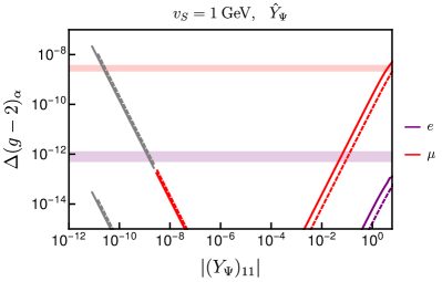
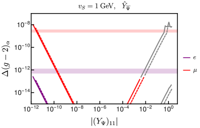
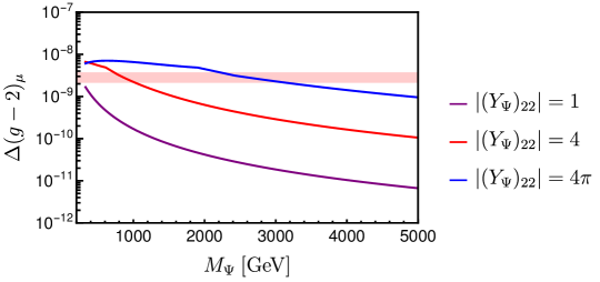
While the BNT model can explain $\Delta(g-2)_{\mu}$, at least one of the Yukawas needs to be ${\cal O}(1)$, given current lower limits on the heavy fermion masses. In fact, as we show in figure 7, in the BNT model one can derive an upper bound on the mass of $\Psi$, from the requirement that the experimental anomaly is correctly explained. As figure 7 demonstrates, even for $|(Y_{\Psi})_{22}|=4\pi$, $m_{\Psi}$ can not be larger than roughly 3 TeV in this case. Note that such a large coupling makes the model non-perturbative, thus this number is conservative and the LHC should be able to test values up to $|(Y_{\Psi})_{22}|\sim(6-7)$.

3.2 Results for the BNT$\phi$ model

Figure 8: $\Delta(g-2)_{\alpha}$ as a function of $m_{\phi}$ for different values of $v_{\phi}$ and $Y_{e\phi}=Y_{e\phi^{c}}$. The coloured lines are the numerical result, the gray lines are calculated with the approximation formulas, see text. Full lines are calculated with $(Y_{e\phi})_{11}=0.06$ and $(Y_{e\phi})_{22}=1$, dashed lines $(Y_{e\phi})_{11}=0.006$ and $(Y_{e\phi})_{22}=0.1$. As in all other figures in this section, red is for $\mu$ and purple for $e$.

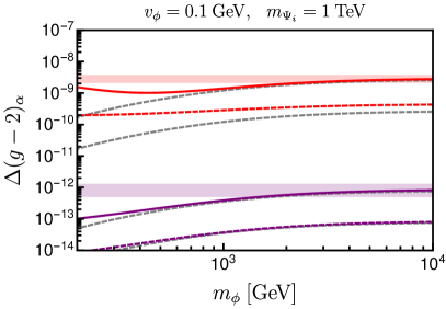
Let us turn now to a discussion of the extended BNT model. The addition of the scalar $\phi$ to the model generates diagrams, for which the mass flip, necessary for the generation of $\Delta(g-2)_{\alpha}$, can be caused by the large fermion mass internal to the loop.

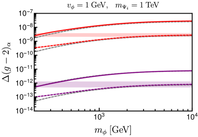
Figure 8 shows a comparison of the approximation formulas, see section 2, to the full numerical results from SPheno. The plot shows $\Delta(g-2)_{\alpha}$ as a function of $m_{\phi}$ for different values of $v_{\phi}$ and $Y_{e\phi}=Y_{e\phi^{c}}$. The neutrino fit was done with a diagonal coupling $Y_{\Psi}$, with entries on the diagonal equal to $(Y_{\Psi})_{ii}=1$ for simplicity. The plots demonstrate that there is a large range of parameter space, for which both experimental anomalies can be explained simultaneously. It may seem counter-intuitive that $\Delta(g-2)_{\alpha}$ rises with increasing mass $m_{\phi}$. The reason for this is the relative sign between the diagrams from the Goldstones and the scalars, see eq. (2.4). This sign leads to a cancellation in $\Delta(g-2)_{\alpha}$ if the scalars $h^{0}$ and $\phi^{+}$ are degenerate with the corresponding Goldstone bosons. For large $m_{\phi}$ this cancellation is less effective and in the limit $m_{\phi}\to\infty$, only the Goldstone diagrams contribute to the observable.

Figure 8 also demonstrates that the approximation formulas work quite well for $v_{\phi}$ order ${\cal O}({\rm GeV})$, as expected. For the muon, the approximation formula starts to differ from the numerical results, once $v_{\phi}$ and $Y_{e\phi}$ are smaller than GeV and $Y_{e\phi}\ll 1$, respectively, while for the electron the approximation still works reasonably. Again, this is to be expected, since $m_{\mu}/m_{e}\simeq 200$, such that diagrams with external mass flips are more important in the case of the muon. Depending on other model parameters, the diagrams proportional to $v_{\phi}$ will be sub-dominant even for very large (i.e. non-perturbative) Yukawa couplings for $v_{\phi}\raise 1.29167pt\hbox{$\;<$\kern-7.5pt\raise-4.73611pt\hbox{$\sim\;$}}(10^{-3}-10^{-2})$ GeV. For $v_{\phi}$ below $10^{-3}$ GeV the model can not explain $\Delta(g-2)_{e}$ and the results of the original BNT model are approximately recovered.

Figure 9: $\Delta(g-2)_{\alpha}$, the shift with respect to the standard model value of $(g-2)_{\alpha}$, as a function of $m_{\Psi}$. The mass of the scalar $\phi$ are $m_{\phi}=1$ TeV (left) and $m_{\phi}=10$ TeV (right). The neutrino data is fitted with a diagonal $Y_{\Psi}$ and the factor $f$ has been chosen $f\simeq 0.06$ to fit the two experimental anomalies at the same value of $m_{\Psi}$. This is neither necessary nor a prediction of the model and has been done only for demonstration. The points have been calculated assuming $Y_{e\phi}=Y_{e\phi^{c}}$ and the full dashed lines are for $(Y_{e\phi})_{ii}=1$, dashed lines for $(Y_{e\phi})_{ii}=4\pi$.

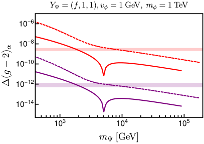
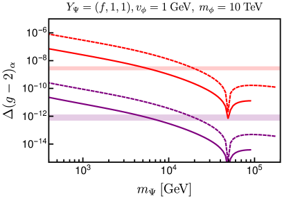
Since roughly $\Delta(g-2)_{\alpha}\propto 1/m_{\Psi}$, explaining correctly the experimental anomalies would imply an upper limit on $m_{\Psi}$. The most conservative value for this limit is reached, if all Yukawa couplings take the maximum value allowed by perturbativity. Taking $\forall Y\sim(4\pi)$ the result is roughly of order $m_{\Psi}\sim{\cal O}(100)$ TeV. This number is so large, that it is only of academic interest. Figure 9 shows that for large $m_{\phi}$, say $m_{\phi}$ larger than 1 TeV, there is practically no dependence on the choice of $m_{\phi}$. The reason for this is that in this limit, all the heavy scalar states decouple from the calculation and the only contribution to the observable comes from the Goldstone diagrams.

Figure 9 also demonstrates, that for more reasonable couplings again the upper limit on $m_{\Psi}$ is much lower. Allowing $Y_{e\phi}=4\pi$, but restricting $Y_{\Psi}$ to order ${\cal O}(1)$ the limit is roughly $(8-10)$ TeV, while for all couplings no larger than $1$, one finds $m_{\Psi}\leq(2-3)$ TeV. This last number is close to what the LHC can probe in the high luminosity run, although the LHC will not be able to cover the allowed range of masses completely, see next section.

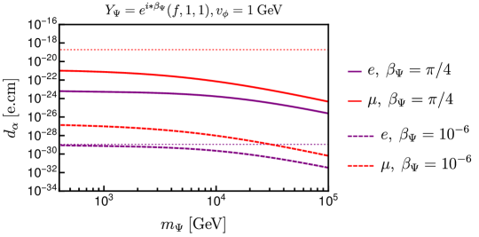
Let us briefly discuss the electric dipole moments, $d_{\alpha}$. Figure 10 shows one example as function of $m_{\Psi}$. The couplings $Y_{e\phi}$, $Y_{e\phi^{c}}$ have been taken real and equal to one, $Y_{e\phi}=Y_{e\phi^{c}}=1$. The plot shows that $d_{e}$ provides a severe constraint, while for $d_{\mu}$ there is no part of the parameter space, where the model can saturate the experimental bound. The plot uses the same parameters and fitting as was used in figure 9 for the $\Delta(g-2)_{\alpha}$. $d_{e}$ probes phases as low as $10^{-6}$. Thus, the large couplings needed to explain $\Delta(g-2)_{e}$ essentially need to be real.

For the BNT$\phi$ model, in order to generate the CP-phase $\delta$ in the neutrino fit, one can always put the phases into the small Yukawa coupling. (In the case of figure 10 taken to be $Y_{\overline{\Psi}}$). Thus, the model can survive the $d_{e}$ constraint easily, but also does not make any testable predictions.

Figure 10: $d_{\alpha}$, the electric dipole moments, as a function of $m_{\Psi}$. The large couplings, except $(Y_{\Psi})_{11}$, have all been taken to be equal to 1 in this plot.

Figure 11: Br$(l_{i}\to l_{j}\gamma)$ as a function of $m_{\Psi}$. The large couplings have all been taken to be equal to 1 in this plot. For the parametrization of $Y_{\Psi}$ see text.

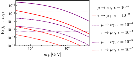
The large couplings not only have to be real, they also have to be close to diagonal, as figure 11 demonstrates. Here, $Y_{\Psi}$ has simply be parametrized as:

$$Y_{\Psi}=\begin{pmatrix}f&\epsilon&\epsilon\\ \epsilon&1&\epsilon\\ \epsilon&\epsilon&1\\ \end{pmatrix}$$ (49)

Here, $f\simeq 0.06$, as discussed above. $\mu\to e\gamma$ provides a severe constraint on the off-diagonal in the $(12)$ sector: $\epsilon\leq 10^{-(5/6)}$, depending on the mass of $\Psi$. $\tau\to\mu\gamma$ is much less stringent, but still provides $\epsilon\leq 10^{-2}$ for the lowest $m_{\Psi}$.

In summary, the extended version of the BNT model, BNT$\phi$, can explain the experimentally observed anomalies in $(g-2)$, while at the same time fitting neutrino oscillation data, easily in large parts of its parameter space. Electric dipole moments force the large Yukawa coupling, required for $\Delta(g-2)_{\alpha}^{exp}$, to be (nearly) real, while cLFV constrainst require them to be (nearly) diagonal. This has some interesting consequences for the phenomenology of the heavy fermions $\Psi$, as we are going to discuss in the next section.

4 Heavy fermions at colliders

We have calculated the production cross sections for the different heavy fermions of the BNT model using MadGraph [38, 39, 40]. For the pair production of multiply charged particles photon-photon fusion diagrams are especially important at large scalar masses, despite the tiny parton density of the photon inside the proton. Manohar et al. [41, 42] have calculated an updated determination of the photon PDF inside the proton recently. The resulting LUXqed17$\_$plus$\_$PDF4LHC15$\_$nnlo$\_$100 combines QCD partons from PDF4LHC15 [43] with the LUXqed calculation of the photon density. Results for cross sections using this set of PDFs are shown in figure 12 for the LHC and a hypothetical future 100 TeV pp-collider.

Figure 12: Production cross sections for the exotic fermions in the BNT model for the LHC (left) and a future 100 TeV collider (right).

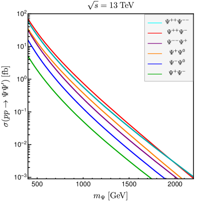
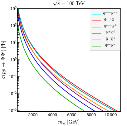
The largest cross sections are pair production of the doubly charged fermions and associated production of $\Psi^{++}\Psi^{-}$. For the high-luminosity LHC with ${\cal L}=3/$ab each of these give more than 100 (20) events for $m_{\Psi}=1.5$ (1.8) TeV before cuts. We expect that therefore, depending on search strategy and backgrounds, the final reach of the LHC for discovery of the heavy fermions of the BNT model should roughly lie in this mass range.

Possible decays of the heavy fermions depend on whether the scalars $S$ and/or $\phi$ are lighter or heavier than $\Psi$. We will concentrate on the case that all new scalars are heavier than the fermions for definiteness. Final states for the different $\Psi$ are: $\Psi^{++}_{i}\to l_{j}^{+}W^{+}$, $\Psi^{+}_{i}\to(l_{j}^{+}Z^{0},l_{j}^{+}h^{0},\nu_{j}+W^{+})$ and $\Psi^{0}_{i}\to(l_{j}^{\pm}+W^{\mp},\nu_{j}+h^{0},\nu_{j}+Z^{0})$. Since $\Psi^{0}_{i}$ are Majorana fermions, both lepton charges should occur with (nearly) equal branching ratios.

Before entering into a more detailed discussion of the different branching ratios, let us comment briefly on existing limits from LHC searches. Several “exotic” searches at ATLAS and CMS can provide lower mass limits on $\Psi$. The currently most stringent one is, to our knowledge, the multi-lepton search by CMS [44]. This work uses a total of $137/$fb of statistics to search for three charged leptons with missing energy in the final state and no hadronic activity associated to the events. The target process is type-III seesaw, the final state searched for can be generated in this model via $pp\to\Sigma^{+}\Sigma^{0}\to(W^{+}\nu)+(W^{+}l^{-})\to l^{+}l^{+}l^{-}\nu\nu$, from the leptonic decays of the $W$s. For $\Sigma$ decaying “flavour-democratically” the lower limit is $m_{\Sigma}=880$ GeV. (This assumes equal branching ratios to the different lepton families. For $\Sigma$ decaying to $\tau$’s the limit is considerably worse, see [44] and for more details the earlier paper [45]). While both, cross sections and branching ratios, are different in the seesaw type-III and the BNT model, a rough estimate using fig.(11) of [44] gives a lower limit on $m_{\Psi}$ in the range of (800-900) GeV for $\Psi^{++}$ decaying to e or $\mu$.

Figure 13: Left: Total width of $\Psi^{++}$ and Br($\mu\to e\gamma$) as function of $v_{S}$. Right: Branching ratios of $\Psi^{++}$. The plot shows some random scan for a fixed mass $m_{\Psi}=1$ TeV, see text.

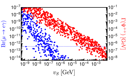
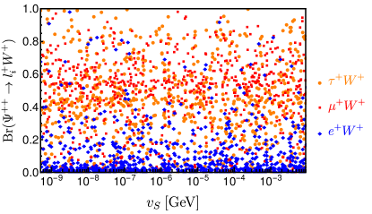
Let us turn now to a discussion of the decay branching ratios of the heavy fermions. As discussed in the previous section, neutrino data requires that at least one of the matrices $Y_{\Psi}$ or $Y_{\overline{\Psi}}$ to be non-diagonal. Since the same couplings are responsible for the decays of the heavy fermions, in general one would expect that the decays of $\Psi^{++}$, $\Psi^{+}$ and $\Psi^{0}$ also violate flavour.

An example is shown in figure 13. Here, we show the total decay width of $\Psi^{++}$ and Br$(\mu\to e\gamma)$ (to the left) as well as the branching ratios Br($\Psi^{++}\to l_{j}^{+}W^{+}$) for $j=e,\mu,\tau$ (right) as function of $v_{S}$. For this figure, we have chosen $m_{\Psi_{1}}=1$ TeV and the neutrino masses were fitted with eq. (46). In this scan we choose randomly the angles in matrix $W$, we restricted the entries in the matrix $T$ to be order ${\cal O}(1)$ on the diagonal and ${\cal O}(10^{-1})$ on the off-diagonal, and for simplicity $K\equiv 0$. Note that, due to the restrictions on $T$, $Y_{\Psi}$ and $Y_{\overline{\Psi}}$ have a similar order of magnitude in this plot. The plot to the left shows that both Br$(\mu\to e\gamma)$ and the total width of $\Psi^{++}$ decrease with increasing $v_{S}$, since larger $v_{S}$ requires smaller Yukawa couplings in the neutrino fit. The plot to the right, however, shows no such tendency in the branching ratios. This is easily understood: While the total width is sensitive to the overall size of the Yukawa couplings, ratios of branching ratios depend only on ratios of Yukawa couplings. Thus, an upper limit on Br$(\mu\to e\gamma)$ does not restrict the possibility to have flavour violating $\Psi^{++}$ decays. Results for the decays of $\Psi^{+}$ and $\Psi^{0}$ show the same qualitative behaviour, we do not repeat these plots here.

The situation is very different in those parts of parameter space, where the model can explain $\Delta(g-2)_{e}$ and obey the upper bound from cLFV decays at the same time. As discussed in the previous section $Y_{\Psi}$ (or $Y_{\overline{\Psi}}$) and $Y_{e\phi}$ must be “large” and nearly diagonal to fit $\Delta(g-2)_{e}$. In this case all heavy fermion decays are very nearly flavour diagonal. We have checked numerically that points with $Y_{\Psi}$ and $Y_{e\phi}$ in the range for giving the correct $\Delta(g-2)_{e}$ can not have measurable flavour violating decays of the heavy fermions without grossly violating existing cLFV bounds.

Figure 14: Branching ratios for the decays of $\Psi^{+}_{1}$ and $\Psi^{0}_{1}$ as a function of $Y_{e\phi}$, for two different values of $v_{\phi}$, $v_{\phi}=1$ GeV (0.1 GeV) full lines (dashed lines). All points in this plot are within the 1$\sigma$ c.l. range of the two experimental anomalies, $\Delta(g-2)_{e}$ and $\Delta(g-2)_{\mu}$. This is achieved by fitting $Y_{\Psi}$ as a function of $Y_{e\phi}$. In this case, all decays are flavour-diagonal, as discussed in the text.

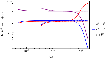
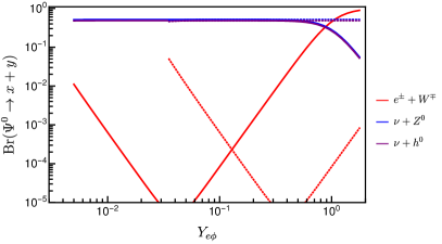
The decays of $\Psi^{+}_{1}$ and $\Psi^{0}_{1}$ depend, moreover, on the value of $v_{\phi}$ and $Y_{e\phi}$. Figure 14 shows an example. In these plot branching ratios are shown as function of $Y_{e\phi}$ for two values of $v_{\phi}$. All points in this plot are within the 1$\sigma$ c.l. range of the two experimental anomalies, $\Delta(g-2)_{e}$ and $\Delta(g-2)_{\mu}$. For values of $v_{\phi}<{\rm(few)}10^{-3}$ GeV $\Delta(g-2)_{e}$ can not be fitted anymore with perturbative Yukawa couplings. The lines stop on the left side, when $Y_{\Psi}$ becomes non-perturbative. Note that $Y_{\Psi}$ is fitted to the experimental data as a function of $Y_{e\phi}$ and thus, $Y_{\Psi}>>Y_{\overline{\Psi}}$ in this calculation.

It is interesting to point out that for $Y_{e\phi}>>Y_{\Psi}$, which occurs only for $v_{\phi}=1$ GeV in these figures, the decays $\Psi^{+}\to e^{+}h^{0}$ and $\Psi^{0}\to e^{\pm}W^{\mp}$ are enhanced. This particular pattern appears only in the BNT$\phi$ model (and not in the original BNT model). One can trace it back analytically to the appearance of the coupling $Y_{e\phi}$ in the coupling of the heavy fermions to the SM Higgs, due to the mixing of $H$ and $\phi$ (proportional to $v_{\phi}/v$).

We note that the model does not predict the hierarchy among the different copies of $\Psi$. Thus, the lightest of these can couple dominantly to either $e$, $\mu$ or $\tau$. Figure 14 shows the case, where the lightest $\Psi$ couples to $e$. The plots for the other cases (coupling to $\mu$ or $\tau$) are very similar and we do not repeat them here.

In summary, the heavy fermions $\Psi$ of the BNT model can be produced at the high-luminosity LHC. While in general one expects to have large LFV decays of the heavy fermions, fitting $\Delta(g-2)_{e}$ to the experimental anomaly, requires large and flavour-diagonal couplings. Thus, in order for the model to explain $\Delta(g-2)_{e}$, the heavy fermions must decay in a flavour conserving manner. Interestingly, also the decays of $\Psi^{+}$ and $\Psi^{0}$ indirectly trace the presence of $\phi$ in the model via enhanced rates for the decays $\Psi^{+}\to e^{+}h^{0}$ and $\Psi^{0}\to e^{\pm}W^{\mp}$, if $Y_{e\phi}$ is the largest Yukawa coupling.

5 Summary

We propose an extension of the original Babu-Nandi-Tavartkiladze (BNT) neutrino model to accommodate the experimental $(g-2)_{\alpha}$ ($\alpha=e,\mu$) anomalies, compatible with neutrino oscillation data and current cLFV bounds. In this model, the presence of an extra hypercharge zero triplet scalar gives a sizeable contribution to the dipole operator proportional to the mass of the exotic heavy fermions. The situation is different for the original BNT model, where the dipole operators are suppressed by the small charged lepton masses. Consequently, the original BNT model can not explain both anomalies at the same time, but $\Delta(g-2)_{\mu}$ could be explained if at least one of the exotic fermions has a mass of roughly $m_{\Psi}\raise 1.29167pt\hbox{$\;<$\kern-7.5pt\raise-4.73611pt\hbox{$\sim\;$}}(2-3)$ TeV, partially within reach of the high-luminosity LHC.

In the extended BNT model, an explanation of both observed anomalies, $(g-2)_{e}$ and $(g-2)_{\mu}$, is compatible with neutrino oscillation data and perturbative couplings in large part of the available parameter space. The smallness of the observed $m_{\nu}$, together with the requirement to explain correctly the $(g-2)$ anomalies, selects a specific part of the parameter space. Specifically, $Y_{e\phi}$ and either $Y_{\Psi}$ or $Y_{\overline{\Psi}}$ have to be order ${\cal O}(0.1-1)$. cLFV bounds then force the large couplings to be (nearly) flavour diagonal. Additional constraints on these couplings come from the current EDM bounds of the electron. We showed that the experimental bound for $\mid d_{e}\mid\sim 1.1\times 10^{-9}e$ cm forces the large couplings, needed to explain $\Delta(g-2)_{e}$, to be mostly real. These results are in agreement with model-independent considerations which can be made based on an effective field theory analysis [17]. For $d_{\mu}$, on the other hand, the model can not give large enough values to saturate the current experimental bound. No observation of $d_{\mu}$ is therefore expected in the current model.

Since cLFV current bounds require the large couplings to be nearly diagonal in order to avoid large cLFV observables, decays of the heavy fermions are necessarily flavour conserving. We disussed the decays of $(\Psi^{0},\Psi^{+},\Psi^{++})$ for the case that the scalars are heavier than the fermions. We have used MadGraph [38, 39, 40] together with the LUXqed PDFs [41, 42] to calculate production cross-sections of the different heavy fermions for the LHC and a possible future $\sqrt{s}=100$ TeV hadron collider. For the high-luminosity LHC, future searches for the heavy fermions of the BNT model can probe masses up to roughly $m_{\Psi}\leq(1.5-1.8)$ TeV.

We discussed branching ratios of the heavy fermions. $\Psi_{\alpha}^{++}$ decay via $\Psi_{\alpha}^{++}\rightarrow l_{\alpha}^{+}W^{+}$ with $100\%$, whereas $\Psi_{\alpha}^{+}\rightarrow(l_{\alpha}^{+}h^{0},l_{\alpha}^{+}Z^{0},\nu W^{+})$. The branching ratio to $l_{\alpha}^{+}h^{0}$ is enhanced if $Y_{e\phi}\raise 1.29167pt\hbox{$\;>$\kern-7.5pt\raise-4.73611pt\hbox{$\sim\;$}}{\cal O}(1)$. Similarly, for $\Psi^{0}$ decays the branching ratios $\Psi_{\alpha}^{0}\rightarrow l_{\alpha}^{\pm}W^{\pm}$ can be large in the same parts of parameter space. In summary, the extended BNT$\phi$ model can explain the observed anomalies in $(g-2)$, while making interesting predictions for the decay patterns of the exotic fermions.

Acknowledgements

Work supported by the Spanish grants FPA2017-85216-P (MINECO/AEI/FEDER, UE) and PROMETEO/2018/165 grants (Generalitat Valenciana). R.C. is also supported by FPU15/03158. R.F. acknowledges the financial support from the Grant Agency of the Czech Republic (GAČR) through contract number 20-17490S and from the Charles University Research Center UNCE/SCI/013. C.A. is supported by FONDECYT-Chile grant No. 11180722 and ANID-Chile PIA/APOYO AFB 180002.

Appendix A Appendix: Full Lagrangian expression

The full expression of the extra interactions and mass terms of the ${\rm BNT}{\phi}$ model, including $SU(2)_{L}$ indices ($i$, $j$, …, $p$), is as follows.

$$\mathcal{L}_{{\rm BNT}{\phi}} =M_{\Psi}\Psi_{ij}\overline{\Psi}_{ij}+Y_{\Psi}L_{i}\Psi_{ji}H_{j}^{*}+Y_{\overline{\Psi}}\overline{\Psi}_{lj}L_{m}S_{ijk}\epsilon_{im}\epsilon_{kl}+Y_{e\phi}e^{c}\overline{\Psi}_{ij}\phi_{ji}$$

$$+Y_{e\phi^{c}}e^{c}\overline{\Psi}_{ij}\phi_{ij}^{*}+Y_{\Psi\phi}\Psi_{ij}\overline{\Psi}_{jk}\phi_{ki}+Y_{\Psi\phi^{c}}\Psi_{ij}\overline{\Psi}_{jk}\phi_{ik}^{*}-\mathcal{V}\,,$$ (50)

$$\mathcal{V} =m_{S}^{2}S_{ijk}^{*}S_{ijk}+m_{\phi}^{2}\textrm{Tr}\left(\phi^{\dagger}\phi\right)+\left[\mu_{\phi}^{2}\textrm{Tr}\left(\phi\phi\right)+\textrm{h.c.}\right]+\left[\mu_{H\phi}H^{\dagger}\phi H\right.$$

$$\left.\mu_{S\phi}S_{ijk}^{*}S_{ijl}\phi_{kl}+\textrm{h.c.}\right]+\frac{1}{2}\lambda_{2a}\left(S_{ijk}^{*}S_{ijk}\right)^{2}+\frac{1}{2}\lambda_{2b}S_{ijk}^{*}S_{mno}^{*}S_{ljk}S_{pno}\epsilon_{im}\epsilon_{lp}$$

$$\frac{1}{2}\lambda_{3}\left(H^{\dagger}H\right)S_{ijk}^{*}S_{ijk}+\frac{1}{2}\lambda_{4}H_{j}H_{i}^{*}S_{klm}^{*}S_{nlm}\epsilon_{ik}\epsilon_{jn}+\lambda_{6a}\left(H^{\dagger}H\right)\textrm{Tr}\left(\phi^{\dagger}\phi\right)$$

$$\lambda_{6b}H^{\dagger}\phi\phi^{\dagger}H+\lambda_{7a}\left(S_{ijk}^{*}S_{ijk}\right)\textrm{Tr}\left(\phi^{\dagger}\phi\right)+\lambda_{7b}S_{ijk}^{*}S_{ijn}\left(\phi\phi^{\dagger}\right)_{kn}$$

$$\lambda_{7c}S_{ijk}^{*}S_{ilm}\left(\epsilon\phi^{*}\right)_{jk}\left(\epsilon\phi\right)_{lm}+\lambda_{8a}\left[\textrm{Tr}\left(\phi^{\dagger}\phi\right)\right]^{2}+\lambda_{8b}\textrm{Tr}\left(\phi\phi\phi^{\dagger}\phi^{\dagger}\right)$$

$$\left\{\lambda_{5}H_{i}H_{j}H_{k}S_{ijk}^{*}+\lambda_{9}\left(H^{\dagger}H\right)\textrm{Tr}\left(\phi\phi\right)+\lambda_{10a}S_{ijk}^{*}S_{ijk}\textrm{Tr}\left(\phi\epsilon\phi^{T}\epsilon^{T}\right)\right.$$

$$\left.\lambda_{10b}S_{ijk}^{*}S_{ilm}\left(\epsilon\phi\epsilon^{T}\right)_{lj}\left(\epsilon\phi\epsilon^{T}\right)_{mk}+\lambda_{11}\left[\textrm{Tr}\left(\phi\phi\right)\right]^{2}+\lambda_{12}\textrm{Tr}\left(\phi\phi\right)\textrm{Tr}\left(\phi^{\dagger}\phi\right)+\textrm{h.c.}\right\}\,.$$ (51)

Whenever it was appropriate, we used a vector and matrix notation (in $SU(2)_{L}$ space) for the various fields. As usual, $\epsilon$ stands for the 2-dimensional Levi-Civita tensor.

References

- [1] Super-Kamiokande Collaboration Collaboration, Y. Fukuda et al., “Evidence for oscillation of atmospheric neutrinos,” Phys.Rev.Lett. 81 (1998) 1562–1567, arXiv:hep-ex/9807003 [hep-ex].
- [2] SNO Collaboration Collaboration, Q. Ahmad et al., “Direct evidence for neutrino flavor transformation from neutral current interactions in the Sudbury Neutrino Observatory,” Phys.Rev.Lett. 89 (2002) 011301, arXiv:nucl-ex/0204008 [nucl-ex].
- [3] P. F. de Salas, D. V. Forero, C. A. Ternes, M. Tortola, and J. W. F. Valle, “Status of neutrino oscillations 2018: 3 hint for normal mass ordering and improved CP sensitivity,” Phys. Lett. B782 (2018) 633–640, arXiv:1708.01186 [hep-ph].
- [4] P. de Salas, D. Forero, S. Gariazzo, P. Martínez-Miravé, O. Mena, C. Ternes, M. Tórtola, and J. Valle, “2020 Global reassessment of the neutrino oscillation picture,” arXiv:2006.11237 [hep-ph].
- [5] Muon g-2 Collaboration, H. Brown et al., “Precise measurement of the positive muon anomalous magnetic moment,” Phys. Rev. Lett. 86 (2001) 2227–2231, arXiv:hep-ex/0102017.
- [6] Muon g-2 Collaboration, G. Bennett et al., “Final Report of the Muon E821 Anomalous Magnetic Moment Measurement at BNL,” Phys. Rev. D 73 (2006) 072003, arXiv:hep-ex/0602035.
- [7] F. Jegerlehner and A. Nyffeler, “The Muon g-2,” Phys. Rept. 477 (2009) 1–110, arXiv:0902.3360 [hep-ph].
- [8] Particle Data Group Collaboration, P. A. Zyla et al., “Review of Particle Physics,” Prog. Theor. Exp. Phys. 2020 (2020) 083C01.
- [9] A. Keshavarzi, D. Nomura, and T. Teubner, “Muon and : a new data-based analysis,” Phys. Rev. D 97 no. 11, (2018) 114025, arXiv:1802.02995 [hep-ph].
- [10] Fermilab E989 Collaboration, G. Venanzoni, “The New Muon g2 experiment at Fermilab,” Nucl. Part. Phys. Proc. 273-275 (2016) 584–588, arXiv:1411.2555 [physics.ins-det].
- [11] E34 Collaboration, M. Otani, “Status of the Muon g-2/EDM Experiment at J-PARC (E34),” JPS Conf. Proc. 8 (2015) 025008.
- [12] S. Borsanyi et al., “Leading-order hadronic vacuum polarization contribution to the muon magnetic momentfrom lattice QCD,” arXiv:2002.12347 [hep-lat].
- [13] A. Crivellin, M. Hoferichter, C. A. Manzari, and M. Montull, “Hadronic vacuum polarization: versus global electroweak fits,” arXiv:2003.04886 [hep-ph].
- [14] R. H. Parker, C. Yu, W. Zhong, B. Estey, and H. Müller, “Measurement of the fine-structure constant as a test of the Standard Model,” Science 360 (2018) 191, arXiv:1812.04130 [physics.atom-ph].
- [15] T. Aoyama, T. Kinoshita, and M. Nio, “Revised and Improved Value of the QED Tenth-Order Electron Anomalous Magnetic Moment,” Phys. Rev. D 97 no. 3, (2018) 036001, arXiv:1712.06060 [hep-ph].
- [16] A. Cárcamo Hernández, S. King, H. Lee, and S. Rowley, “Is it possible to explain the muon and electron in a model?,” Phys. Rev. D 101 no. 11, (2020) 11, arXiv:1910.10734 [hep-ph].
- [17] A. Crivellin, M. Hoferichter, and P. Schmidt-Wellenburg, “Combined explanations of and implications for a large muon EDM,” Phys. Rev. D98 no. 11, (2018) 113002, arXiv:1807.11484 [hep-ph].
- [18] I. Dořsner, S. Fajfer, and S. Saad, “ selecting scalar leptoquark solutions for the puzzles,” arXiv:2006.11624 [hep-ph].
- [19] J. Liu, C. E. Wagner, and X.-P. Wang, “A light complex scalar for the electron and muon anomalous magnetic moments,” JHEP 03 (2019) 008, arXiv:1810.11028 [hep-ph].
- [20] B. Dutta and Y. Mimura, “Electron with flavor violation in MSSM,” Phys. Lett. B 790 (2019) 563–567, arXiv:1811.10209 [hep-ph].
- [21] M. Bauer, M. Neubert, S. Renner, M. Schnubel, and A. Thamm, “Axion-like particles, lepton-flavor violation and a new explanation of and ,” Phys. Rev. Lett. 124 no. 21, (2020) 211803, arXiv:1908.00008 [hep-ph].
- [22] G. Hiller, C. Hormigos-Feliu, D. F. Litim, and T. Steudtner, “Anomalous magnetic moments from asymptotic safety,” arXiv:1910.14062 [hep-ph].
- [23] A. Cárcamo Hernández, Y. Hidalgo Velásquez, S. Kovalenko, H. Long, N. A. Pérez-Julve, and V. Vien, “Fermion spectrum and anomalies in a low scale 3-3-1 model,” arXiv:2002.07347 [hep-ph].
- [24] C. Hati, J. Kriewald, J. Orloff, and A. Teixeira, “Anomalies in 8Be nuclear transitions and : towards a minimal combined explanation,” arXiv:2005.00028 [hep-ph].
- [25] C.-H. Chen and T. Nomura, “Electron and muon , radiative neutrino mass, and in a model,” arXiv:2003.07638 [hep-ph].
- [26] L. Calibbi, M. López-Ibáñez, A. Melis, and O. Vives, “Muon and electron and lepton masses in flavor models,” JHEP 06 (2020) 087, arXiv:2003.06633 [hep-ph].
- [27] F. J. Botella, F. Cornet-Gomez, and M. Nebot, “Electron and muon anomalies in general flavour conserving two Higgs doublets models,” arXiv:2006.01934 [hep-ph].
- [28] K.-F. Chen, C.-W. Chiang, and K. Yagyu, “An explanation for the muon and electron anomalies and dark matter,” arXiv:2006.07929 [hep-ph].
- [29] B. Dutta, S. Ghosh, and T. Li, “Explaining , KOTO anomaly and MiniBooNE excess in an extended Higgs model with sterile neutrinos,” arXiv:2006.01319 [hep-ph].
- [30] S. Jana, V. P. K., and S. Saad, “Resolving electron and muon within the 2HDM,” Phys. Rev. D 101 no. 11, (2020) 115037, arXiv:2003.03386 [hep-ph].
- [31] K. S. Babu, S. Nandi, and Z. Tavartkiladze, “New Mechanism for Neutrino Mass Generation and Triply Charged Higgs Bosons at the LHC,” Phys. Rev. D80 (2009) 071702, arXiv:0905.2710 [hep-ph].
- [32] F. Staub, “SARAH 3.2: Dirac Gauginos, UFO output, and more,” Comput. Phys. Commun. 184 (2013) 1792–1809, arXiv:1207.0906 [hep-ph].
- [33] F. Staub, “SARAH 4 : A tool for (not only SUSY) model builders,” Comput. Phys. Commun. 185 (2014) 1773–1790, arXiv:1309.7223 [hep-ph].
- [34] W. Porod, “SPheno, a program for calculating supersymmetric spectra, SUSY particle decays and SUSY particle production at e+ e- colliders,” Comput. Phys. Commun. 153 (2003) 275–315, arXiv:hep-ph/0301101 [hep-ph].
- [35] W. Porod and F. Staub, “SPheno 3.1: Extensions including flavour, CP-phases and models beyond the MSSM,” Comput. Phys. Commun. 183 (2012) 2458–2469, arXiv:1104.1573 [hep-ph].
- [36] I. Cordero-Carrión, M. Hirsch, and A. Vicente, “Master Majorana neutrino mass parametrization,” Phys. Rev. D 99 no. 7, (2019) 075019, arXiv:1812.03896 [hep-ph].
- [37] I. Cordero-Carrión, M. Hirsch, and A. Vicente, “General parametrization of Majorana neutrino mass models,” Phys. Rev. D 101 no. 7, (2020) 075032, arXiv:1912.08858 [hep-ph].
- [38] J. Alwall, P. Demin, S. de Visscher, R. Frederix, M. Herquet, F. Maltoni, T. Plehn, D. L. Rainwater, and T. Stelzer, “MadGraph/MadEvent v4: The New Web Generation,” JHEP 09 (2007) 028, arXiv:0706.2334 [hep-ph].
- [39] J. Alwall, M. Herquet, F. Maltoni, O. Mattelaer, and T. Stelzer, “MadGraph 5 : Going Beyond,” JHEP 1106 (2011) 128, arXiv:1106.0522 [hep-ph].
- [40] J. Alwall, R. Frederix, S. Frixione, V. Hirschi, F. Maltoni, O. Mattelaer, H. S. Shao, T. Stelzer, P. Torrielli, and M. Zaro, “The automated computation of tree-level and next-to-leading order differential cross sections, and their matching to parton shower simulations,” JHEP 07 (2014) 079, arXiv:1405.0301 [hep-ph].
- [41] A. Manohar, P. Nason, G. P. Salam, and G. Zanderighi, “How bright is the proton? A precise determination of the photon parton distribution function,” Phys. Rev. Lett. 117 no. 24, (2016) 242002, arXiv:1607.04266 [hep-ph].
- [42] A. V. Manohar, P. Nason, G. P. Salam, and G. Zanderighi, “The Photon Content of the Proton,” JHEP 12 (2017) 046, arXiv:1708.01256 [hep-ph].
- [43] J. Butterworth et al., “PDF4LHC recommendations for LHC Run II,” J. Phys. G43 (2016) 023001, arXiv:1510.03865 [hep-ph].
- [44] CMS Collaboration, A. M. Sirunyan et al., “Search for physics beyond the standard model in multilepton final states in proton-proton collisions at 13 TeV,” JHEP 03 (2020) 051, arXiv:1911.04968 [hep-ex].
- [45] CMS Collaboration, A. M. Sirunyan et al., “Search for Evidence of the Type-III Seesaw Mechanism in Multilepton Final States in Proton-Proton Collisions at ,” Phys. Rev. Lett. 119 no. 22, (2017) 221802, arXiv:1708.07962 [hep-ex].