Graph Signal Processing for Infrastructure Resilience: Suitability and Future Directions

Abstract

Graph signal processing (GSP) is an emerging field developed for analyzing signals defined on irregular spatial structures modeled as graphs. Given the considerable literature regarding the resilience of infrastructure networks using graph theory, it is not surprising that a number of applications of GSP can be found in the resilience domain. GSP techniques assume that the choice of graphical Fourier transform (GFT) imparts a particular spectral structure on the signal of interest. We assess a number of power distribution systems with respect to metrics of signal structure and identify several correlates to system properties and further demonstrate how these metrics relate to performance of some GSP techniques. We also discuss the feasibility of a data-driven approach that improves these metrics and apply it to a water distribution scenario. Overall, we find that many of the candidate systems analyzed are properly structured in the chosen GFT basis and amenable to GSP techniques, but identify considerable variability and nuance that merits future investigation.

I Introduction

Critical infrastructure systems such as power systems and water distribution are vital components in the safety and security of a nation. These systems are subject to a wide range of failures and disturbances, including component failures, natural phenomena such as severe storm events and earthquakes, and in the increasingly “wired” age of information technology, cyber-events including both malicious attacks and “benign” events caused by unexpected interactions or upgrades [1, 2, 3, 4, 5]. Considerable research and investment have been executed to analyze systems in response to these vulnerabilities, and to develop novel strategies to manage, mitigate, and recover any degradation in performance due to them. Collectively, these efforts have led to the multidisciplinary field of resilience engineering [6, 7, 8] that seeks to formalize these concepts and apply them to real world situations.

Many of the systems of interest in critical infrastructure have a network structure, including lines and buses in a power system, pipes and junctions in water distribution, or roads and intersections in a transportation system. This commonality in network structure has led to extensive investigation of the resilience of these networks using the language of mathematical graph theory. Graph theory models networks as abstract edges and vertices, and numerous studies have been performed to show how graph theoretic properties and metrics relate to resilience in critical infrastructure problems, e.g., [9, 10, 11, 12].

Motivated by spectral graph theory [13] and algebraic approaches to signal processing [14], the field of graph signal processing (GSP) has developed over the past decade to analyze signals defined on irregular spatial structures modeled as graphs [15, 16]. In the context of infrastructure systems, example “graph signals” include complex phasors on buses in power systems and hydraulic pressure in water distribution systems. Several applications of GSP to infrastructure systems have appeared in the literature, including sensor placement problems [17, 18, 19], false data injection (FDI) [20, 21], and general monitoring problems [22, 23]. More broadly, GSP generalizes techniques from signal processing that could find wide utility in analysis and estimation problems of graph signals in infrastructure applications, see e.g., [24, 25, 26].

Enthusiasm for this potentially powerful set of tools must be tempered by the fact that there exists a number of potential approaches to generalizing Fourier-based techniques to graph signals (i.e., there are numerous “natural” ways to define a graphical Fourier transform (GFT)), and each GSP technique ultimately relies upon some assumption or constraint imposed on the graph signals by this GFT. Furthermore, most of the GSP power systems literature consider at best a few different networks, typically of small ($\lesssim$ 100 buses), and no broad analysis across many systems of different scales has been performed. To this end, in this paper we analyze particular choices of GFT in the context of a number of different infrastructure systems to assess how strongly they meet implied GSP assumptions, and then assess the efficacy of some GSP techniques to understand the impact of these assumptions. This analytical case-study of GSP techniques mirror what must be performed in any practical, real-world application of these techniques to critical infrastructure.

In the following sections, we first review some graph theoretic and GSP preliminaries and discuss some applications of techniques from the field of GSP to signals defined on infrastructure networks. We then move to a more in-depth analysis of the suitability of these techniques for power systems, by considering power-flow analyses of a large set of diverse power networks and relate some relevant GSP signal metrics to the efficacy of proposed GSP techniques. Next, we discuss how the physics of water distribution potentially limits the usage of GSP in that domain and offer an attempt to find a usable GFT. We conclude with additional discussion and future directions for GSP in critical infrastructure.

II Background

II-A Graph Theory Preliminaries

Mathematically, a (undirected) graph $\mathcal{G}=(\mathcal{V},\mathcal{E})$ is defined as a collection of a set of vertices (sometimes called nodes) $\mathcal{V}=\{v_{1},\dots,v_{N}\}$ and a set of edges $\mathcal{E}=\{\{u,v\}:u,v\in\mathcal{V}\}$. $\mathcal{G}$ is said to have $N$ vertices and $|E(G)|=M$ edges. If $\{u,v\}\in\mathcal{E}$, then $u$ and $v$ are said to be adjacent. Given a vertex $v\in\mathcal{V}$, the degree of $v$ is $d(v)=|\{u:\{u,v\}\in\mathcal{E}\}|$, or the number of nodes adjacent to $v$. A directed graph is a graph where the edges are ordered pairs of vertices rather than sets. In other words, $\mathcal{E}=\{(u,v):u,v\in\mathcal{V}\}$. The head of edge $(u,v)$ is $v$ and the tail is $u$. Graphs can also have vertex and/or edge attributes associated with them. In the context of this paper, we are interested in edge weighted graphs, where each edge $e_{k}$ in $\mathcal{E}$ has an associated weight $w_{k}$, or vertex weighted graphs, where each vertex $v_{k}$ has an associated weight $w_{k}$.

The adjacency matrix, $\bm{A}$, is one convenient way of representing the structure of a graph where element $A_{k\ell}=1$ (or the edge weight for edge weighted graphs) if $v_{k}$ is adjacent to $v_{\ell}$ and $A_{k\ell}=0$ otherwise. Note that $\bm{A}$ is symmetric if $\mathcal{G}$ is undirected, but $\bm{A}$ need not be symmetric if $\mathcal{G}$ is directed. The incidence matrix, $\bm{B}$, is another way of storing structural information. For an undirected graph, it is an $N\times M$ matrix where element $B_{k\ell}=1$ if vertex $v_{k}$ is an element of edge $e_{\ell}$ and $B_{k\ell}=0$ otherwise. For a directed graph, element $B_{k\ell}=1$ if $v_{k}$ is the head of $e_{\ell}$, and $B_{k\ell}$ is -1 if it is the tail. For edge weighted graphs, the $\pm 1$ entries of $B$ are replaced with $\pm w_{\ell}$. For undirected graphs, the Laplacian matrix, $\bm{L}$, can be calculated from the adjacency matrix. Specifically, it is defined as $\bm{L}=\bm{D}-\bm{A}$ where $\bm{D}$ is a diagonal matrix such that $D_{kk}=d(v_{k})$ for vertex $k$ and $\bm{A}$ is the adjacency matrix. It is common to consider the spectrum, or the set of eigenvalues $\lambda_{k}$ of $\bm{L}$, to understand certain properties of the graph such as clustering, and for positive weighted, undirected graphs, $\lambda_{k}\geq 0$ [13]. For directed graphs or graphs with negative or complex-valued weights, we will use the underlying positive, undirected adjacency matrix $\bm{A}^{(|u|)}$ where $A^{(|u|)}_{k\ell}=\max\{|A_{k\ell}|,|A_{\ell k}|\}$ [27, 28] to derive a corresponding underlying $\bm{L}^{(|u|)}$. Other generalizations of graph Laplacians exist in the literature, as well [29].

II-B Graph Signal Processing

GSP is a field that has emerged over the past decade and aims to generalize signal processing techniques to signals defined over graphs [16, 15]. In classical signal processing, signals live in a Euclidean space, as for example signals defined over time, images, and video. In GSP, the nodes of a graph define the domain of the so-called graph signal Formally, given a graph $\mathcal{G}=(\mathcal{V},\mathcal{E})$, a graph signal $\bm{f}:\mathcal{V}\to\mathbb{V}$ is a function defined on the vertices of $\mathcal{G}$ that takes values in some vector space $\mathbb{V}$, typically $\mathbb{R}^{N}$, although $\mathbb{C}^{N}$ is a natural domain for power applications. For notational convenience we will denote graph functions $\bm{f}(v_{k})$ by $f_{k}$ emphasizing that the function can indeed be viewed as a vector “attached” to a graph. Several analysis techniques and transforms from classical signal processing have been adapted to signals defined over a graph. Key to these ideas is the notion of an $N\times N$ (possibly complex) GFT matrix $\bm{U}$ that defines the GFT $\tilde{\bm{f}}=\bm{U}^{\dagger}\bm{f}$, where $\dagger$ denotes conjugate-transposition. When $\bm{U}$ is unitary, its columns $\bm{U}_{k}$ are orthonormal and there is a natural inverse GFT defined by $\bm{f}=\bm{U}\tilde{\bm{f}}$. This orthogonality captures much of the original intuition behind the discrete time Fourier transform and is exploited throughout GSP applications. Figure 1 shows some example graph signals and their representations in the GFT domain.

Figure 1: Example graph signals (left column) and their representations in the GFT domain (right column). White noise signals are random on the graph and are uniform in the GFT domain. Low-pass graph signals vary smoothly with respect to the graph topology, and are concentrated in the low-frequency graph harmonics. Sparse signals can have high-frequency graph components and appear seemingly random in the graph domain, but are highly structured in the GFT domain.

There are many ways to define a GFT from a given graph $\mathcal{G}$, some of which do not necessarily produce a unitary transform. Some approaches more motivated by algebraic signal processing use $\bm{A}$ directly, while others exploit spectral graph theoretic motivation of Laplacians [16, 15, 27, 28]. Here, we will restrict ourselves to Laplacian-derived unitary GFT s. For undirected graphs with positive edges, the Laplacian $\bm{L}$ admits the eigendecomposition $\bm{L}=\bm{U}\bm{\Lambda}\bm{U}^{T}$, where $\bm{U}$ is the matrix with its eigenvectors $\bm{U}_{k}$ along its columns and $\bm{\Lambda}$ is a diagonal matrix of the eigenvalues, $0=\lambda_{1}\leq\cdots\leq\lambda_{N}$. For general graphs, $\bm{L}^{(|u|)}$ can be used to define similar transforms [27, 28]. The eigenvalues $\lambda_{k}$ of $\bm{L}$ are used to define a notion of frequency for the graph harmonics defined by eigenvectors $\bm{U}_{k}$. Unlike standard Fourier analysis, these “frequencies” are not uniformly spaced, but they can be ordered. In particular, the harmonics corresponding to $\lambda_{k}=0$ correspond to the average value for that connected component. In the GSP context, the GFT provides an illustration of alignment or smoothness between the graph signals and their adjacent graph edges in much the same way that frequency content of a signal in standard Fourier analysis does. An important measure is the total variation (TV) of a graph signal, defined as $TV(\bm{f})=\bm{f}^{\dagger}\bm{L}\bm{f}=\sum_{k,\ell=1,\ell>k}^{N}A_{k\ell}|f_{k}-f_{\ell}|^{2}$. In the context of the eigendecomposition of $\bm{L}$, TV is the average frequency weighted by the GFT power spectrum of $\bm{f}$.

Another important concept in GSP is that of a graph filter, where a graph signal $\bm{f}$ is modified in the GFT domain and transformed back into the graph signal domain, which can be expressed as $\hat{\bm{f}}=\bm{U}\text{diag}(\bm{h})\bm{U}^{\dagger}\bm{f}$ where the vector $\bm{h}$ re-scales (and/or phase-shifts) the signal energy in each GFT harmonic, in analogy with window methods in classical signal processing. For example $\bm{h}=[1,1,\cdots,1,0,0,\cdots 0]^{\top}$ defines a low-pass graph filter, since all the harmonics above some graph frequency cutoff are set to zero.

III Applications in Resilience

Despite its relative nascence, the field of GSP has rapidly generalized a number of techniques from “standard” signal processing to functions defined on the nodes of a graph, many of which appear to be suitable for infrastructure applications. These include signal denoising [25] and more generally filtering of noisy signal $\breve{\bm{f}}=\bm{f}+\bm{n}$, where $\bm{n}$ is some noise graph process. Much like classical signal processing, the idea is to apply some graph filter $\bm{h}$ that removes as much of $\bm{n}$ while preserving $\bm{f}$, or otherwise extracting spectral components of $\breve{\bm{f}}$. Similarly, when there is both noise and an external FDI signal $\bm{e}$ (so $\breve{\bm{f}}=\bm{f}+\bm{n}+\bm{e}$), a graph filter $\bm{h}$ that extracts the expected spectral content of $\bm{f}$ and $\bm{n}$ can be used to identify potential attacks $\bm{e}$ [20, 21]. When $\bm{f}$ is expected to be sparse (i.e., $\tilde{\bm{f}}$ is concentrated in a few harmonics), this signal structure can be exploited to estimate $\bm{f}$ using only the values at a few vertices [24, 25].

III-A GSP as a signal model

The efficacy of any of the aforementioned GSP techniques is dependent upon the choice of the GFT used. It is assumed that the class of expected or typical signals will have some general structure with respect to the chosen GFT, typically “low-pass” or spectrally sparse in the chosen GFT domain (see Figure 1). If, for example, the typical graph signals are uniformly spread (i.e., “white” noise) with respect to a given GFT, then these GSP techniques will not be as effective. For example, FDI detection would basically devolve into detection based on individual nodes, rather than the entire signal. Such a test would be less sensitive than under the low-pass model, which compares signal energy at the high frequency harmonics in the GFT domain with expected values based on typical signal smoothness. This improves the detection rate of the test by exploiting the overall assumption of signal smoothness. In this sense, the assumption of a particular signal model in a specific GFT domain needs to be evaluated for the specific network and “typical” signals defined on it.

Many of these problems have been addressed under alternative approaches and signal models, for example using compressive sensing (CS) and sparse optimization approaches [30] or data-driven approaches based on e.g., principal component analysis (PCA) [31]. Sparsity inducing bases for CS models and the principal component vectors can both be viewed as unitary matrices that define transforms that induce a signal structure, much like a GFT. Comparison to these two classes of approaches elucidates what the GSP framework is actually assuming, namely, that the network structure and some underlying physical model induces a particular signal structure that can be inferred using only the network structure. This is a stronger assumption than the PCA approach, which exploits the existence of signal structure determined empirically, and on par with many CS approaches where the sparse basis is known a priori. This is not meant to be taken as a criticism of GSP approaches, as it might initially seem that we are advocating for more direct data-driven approaches that more rigidly (at least empirically) induce the signal structure assumptions exploited in the various techniques above. Instead, these GSP motivated approaches attempt to capture something “universal” and physically motivated about a particular class of infrastructure systems.

IV Power Systems

A number of GSP applications can be found in the domain of power systems, at least partially due to the rich set of potential graph models to use for exploitable signal structure. Modeling the graph as unweighted uses only connectivity and ignores all information about the lines themselves, and due to this, appears to be unused in this domain. In [23] the inverse of the length of each line in the power system is used to weight the edges. The decoupled (DC) power flow assumptions imply a graph weighted by the inverse of the reactance (and a graph signal of phases). The above discussion highlights a combinatorial issue that needs to be resolved in order to effectively apply GSP techniques, as one must find both a (weighted) graphical structure and a corresponding GFT operator that effectively induces the desired exploitable signal structure. Just because one combination of network weights and GFT does not appear to induce the required structure does not rule out the existence of a useful model.

Here, we consider weights motivated by (idealized) alternating current (AC) power flow by defining the admittance $y_{k,\ell}=(r_{k,\ell}+jx_{k,\ell})^{-1}$ of a line in terms of the resistance $r_{k,\ell}$ and reactance $x_{k,\ell}$. The current flow $i_{k,l}$ through a line is related to the admittance and the bus voltages $V_{k}$ and $V_{\ell}$ via $i_{k,\ell}=y_{k,\ell}(V_{k}-V_{\ell})$. By assigning a fixed (yet arbitrary) direction to each line, this set of equations can be used to define a directed incidence matrix $\bm{B}_{AC}$ that relates the vector of currents on each edge $\bm{i}$ to the vector of voltages $\bm{V}$ by $\bm{i}=\bm{B}_{AC}^{\dagger}\bm{V}$.

In what follows, we restrict ourselves to analyzing the complex vector of bus voltages, $\bm{V}$, using the AC power flow network structure under the GFT defined by $\bm{L}^{(|u|)}$ for $\bm{B}_{AC}$. Using this as the basis for our GSP analysis, we consider AC power-flow simulations computed by MATPOWER [32] using the example networks provided by that package. We restrict our analyses to networks with bus counts less than 4096 to produce a set of default bus voltages to serve as graph signals. This set of 43 networks spans 4–3374 buses, and includes both IEEE test cases (14, 24, 30, 57, 118, 145, 300 bus cases) and systems modeling complex, real world networks from Texas, France, and Poland, see [32] source code.

IV-A Suitability of GSP Approaches

As discussed in Sec. III-A, a common assumption about the signal structure for GSP applications is that the signal is in some sense compressible, which means that the signal is well approximated by a few GFT harmonics. Let us first define three metrics to illustrate when GSP approaches may be suitable for our analysis problem of choice. The first metric we consider is low-pass compressibility, which is defined by the number of consecutive low-frequency graph Fourier harmonics required to capture some fraction of the overall signal power, here 90% and 99.9%. Low-pass compressible graph signals would be ideal candidates for denoising via a low-pass graph filter. Additionally, low-pass compressibility is exploited in FDI detection approaches; for example the 99.9% threshold was used in [23] as a cutoff for high-pass graph filter to detect FDI. The second metric we consider is general compressibility, which is defined by the minimum number of harmonics required to capture the desired fraction of energy, without the low-pass constraint. Thus, general compressibility is a metric of signal sparsity in the GFT domain. Graph signals that are sparse can be reconstructed from fewer measurements, and this can be exploited to reduce the number of sensors required to monitor the system. The difference between low-pass compressibility and compressibility (i.e., sparsity) can be seen in Figure 1. The third metric we use is total variation $TV(\bm{V})$, an alternative notion of signal smoothness that is commonly encountered in the GSP literature as a regularizer in optimization problems. To normalize the above metrics, we divide the notions of compressibility by the number of buses to compute compressibility ratios, and we normalize $TV(\bm{V})$ by dividing by $||\bm{V}||^{2}$ for each graph signal.

For each network in our MATPOWER test set, we used the default AC power-flow result to assess its low-pass and general compressibility. Figure 2 (top) shows the compressibility ratios for each graph signal. This indicates that many of these signals are reasonably compressible (especially at the 90% threshold) and are generally inversely correlated with network size ($r_{s}=-0.99$, $p=3.9\times 10^{-38}$ for 90% and $r_{s}=-0.53$, $p=2.3\times 10^{-4}$ for 99.9% using Spearman’s rank correlation coefficient $r_{s}$ [33]). The general compressibility notions are similarly correlated. It turns out, however, that these bus voltages are dominated by the average voltage across the entire bus (c.f., the DC approximation) which is captured by the $\lambda=0$ graph harmonic. When we look at the compressibility of only the remaining harmonics, i.e., the perturbations from the signal mean, we see that the signals are far less compressible, see Figure 2 (bottom). The discrepancy between these two panels indicates that sparse reconstruction (equivalently, sparse sensor placement) problems that care only about perturbations from the mean will require more measurements to reconstruct to the same level of error, as the compressibility ratio of a signal essentially determines the number of measurements required to reconstruct the signal at a given error threshold.

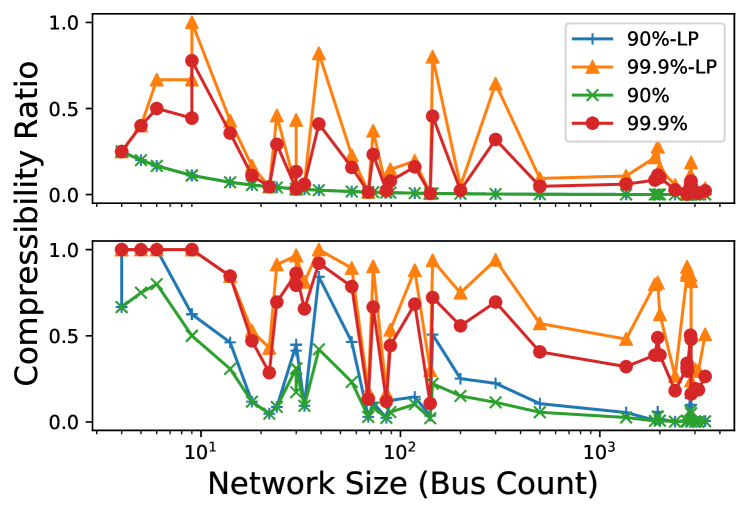
Figure 2: Low-pass (LP) and general compressibility ratios of bus voltages at 90% and 99.9% thresholds. Top: Compressibility ratios of the complete signal. Bottom: Compressibility ratios with the signal average removed.

Figure 3 shows the normalized TV for each of the MATPOWER test cases. Unlike the low-pass and general compressibility which was inversely correlated with network size, here we see that TV is not particularly correlated with network size ($r_{s}=0.19$, $p=0.22$). The largest outlier in Figure 3 corresponds to the IEEE 145 bus, 50 generator dynamic test case, in which over a third of the buses have active generation capability. Motivated by this observation, we performed a correlation analysis that related percentage of buses with active generation to normalized TV and we found a moderately strong correlation ($r_{s}=0.44$, $p=2.9\times 10^{-3}$). Since distributed power generation capability injects extra “degrees of freedom” in the power flow computations, it is not surprising that this produces signals that are in some sense less smooth. Performing a similar analysis indicate that compressibility at the 99.9% threshold is not statistically significantly correlated ($r_{s}=-0.17$, $p=0.25$, for low-pass, $r_{s}=-0.28$, $p=0.07$ for general), but that 90% compressibility is (both $r_{s}=-0.83$, $p=3.38\times 10^{-12}$), albeit less strongly correlated than they are to network size.

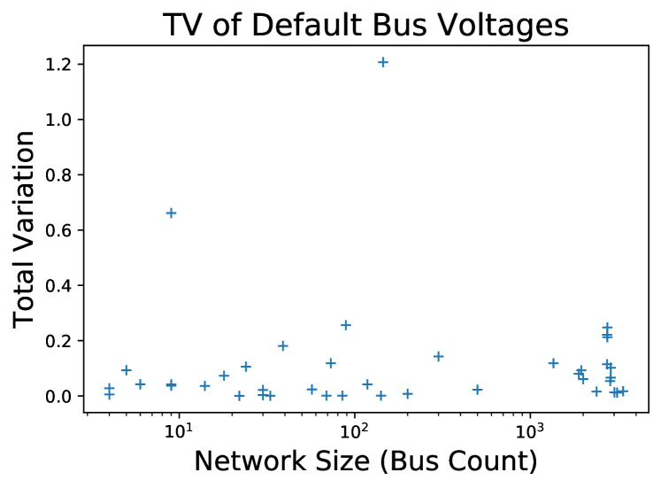
Figure 3: Total Variation of AC power flow-computed bus voltages compared to network size.

IV-B Impact on GSP Techniques

The previous section focused on how well the set of candidate systems and signals met some common GSP-motivated signal models. In this section, we analyze some GSP techniques applied to the same set of systems and signals to assess the impacts of the metrics from the previous section on these approaches. Applications related to sparse reconstruction and approximation, such as the optimal sensor placement problem have already been discussed at a notional level in the context of Figure 2, so we will instead focus on estimating the true bus voltages from those corrupted by noise (the denoising problem) and FDI s.

Two approaches to the denoising problem are considered here. The first is to use the $99.9\%$ low-pass compression threshold for a graph low-pass filter $\bm{h}_{LP}$, where $h_{LP_{k}}=1$ for harmonics below the threshold and $h_{LP_{k}}=0$ for those above it. The second denoising approach uses a graph filter $\bm{h}_{\alpha}$ determined by TV regularization approach parameterized by $\alpha$, where $\bm{h}_{\alpha_{k}}=(1+2\alpha\lambda_{k})^{-1}$ for the eigenvalues $\lambda_{k}$ of each network’s $\bm{L}^{(|u|)}$ [26]. To assess the efficacy of these filters, for each of the power systems and default bus voltages $\bm{V}$, we performed a series of Monte Carlo simulations on these two forms of denoising. For each default voltage signal $\bm{V}$, we added a white noise signal $\bm{n}$ so that the expected signal-to-noise ratio (SNR) was $20$ dB, and then performed the denoising procedure for $\bm{h}_{LP}$ and $\bm{h}_{\alpha}$ for 50 logarithmically spaced $\alpha\in[.01,10]$. This procedure was repeated for 25 independent noise perturbations per network, and the improvement (possibly negative) in output SNR was computed. Figure 4 (top) shows the average improvement in SNR across these random samples for the best (over $\alpha$) $\bm{h}_{\alpha}$ with the bottom panel showing the best $\alpha$ for that network. We see that TV correlates with these two quantities quite well (SNR gain: $r_{s}=-0.57$, $p=6.7\times 10^{-5}$, best $\alpha$: $r_{s}=-0.75$, $p=1.0\times 10^{-8}$) indicates a strong inverse correlation between the TV of the noiseless signal and improvement in SNR by the denoising procedure. Furthermore, we find that the best $\bm{h}_{\alpha}$ improved the SNR by about $1.3~{}dB$ more on average than $\bm{h}_{LP}$, although other compression ratios may perform better.

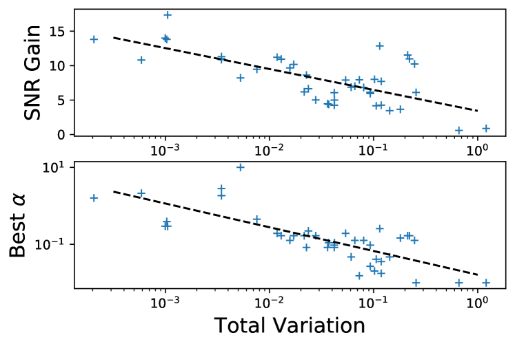
Figure 4: Top: SNR Gain of denoising vs. TV, using best $\bm{h}_{\alpha}$ for each network Bottom: Best $\alpha$ for each network vs. TV. Dashed lines show log-linear and log-log regression fits indicating overall inverse correlation.

Next, we consider how the GSP model assumptions relate to FDI detection. The approach of [23] is based on the high-pass filtering of a signal $\bm{f}$ perturbed by noise $\bm{n}$ and an injected graph signal $\bm{e}$. Thresholding on the norm of the filtered signal is used to determine the presence of an FDI attack. To assess how this approach might work with respect to the systems here, we define a high-pass filter $\bm{h}_{HP}=1-\bm{h}_{LP}$, using the low-pass filters derived from the 99.9% compressibility thresholds above. We then apply this filter to graph signals $\bm{\delta}_{k}$ where $\bm{\delta}_{k}=1$ on $k^{th}$vertex and 0 elsewhere. This measures how much injected signal will contribute to the detection threshold (i.e., the closer the filtered norm is to 1, the more detectable an FDI on that vertex will be). Figure 5 shows the median norm of the filtered $\bm{\delta}_{k}$ for each network (sorted by 99.9% low-pass compressibility ratio), along with notions of the spread of the resulting distributions of the norms. There is a strong correlation between the median and compressibility ($r_{s}=-0.99$, $p=1.7\times 10^{-34}$), but it is worth noting that there is substantial variability for many of the networks. This indicates that certain buses are more susceptible to FDI attacks than others.

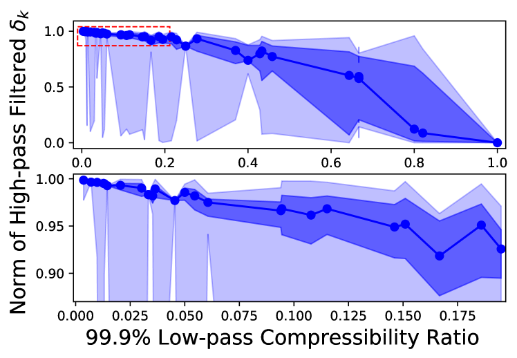
Figure 5: Top: Norm of $\bm{\delta}_{k}$ filtered using $\bm{h}_{HP}$. Line is the median for each network, darker shaded region is the inner 50% quantile, lighter shaded region is the full range. Bottom: Zoomed-in view of dashed rectangle from top panel.

V Water Distribution Systems

Unlike power systems, water systems do not appear to have the variety of GSP-motivated analysis in the literature. The exception appears to be the work in [34, 19] which focuses on the spread of pollutants in water distribution systems. The authors note that the graph Fourier structure of the pollutant “signal” is not sparse or compressible with respect to the Laplacian of the unweighted network model. This lack of signal structure in the graphical Fourier domain led to the development of so-called “data-driven” approaches to designing GFT s that induce the desired compressibility based on a collection of observed data [34, 19]. However, these techniques more closely resemble the PCA-based analysis discussed in Sec. III-A than GSP, and do account for the structure of the underlying network.

We conjecture that part of the reason for a lack of GSP analysis in this domain is the absence of canonical relations between signals on the graph vertices and flows on the graph edges, unlike the power systems case. There is, however, an analogy between hydraulic and electric circuits that associates flow-volume through pipes with current through branches, and pressure differences between junctions with voltage differences between buses. Unlike Ohm’s law between voltage and current, the hydraulic circuit equation for pressure loss is generally modeled as nonlinear and include a number of additional physical considerations that make the equations less tractable than in power systems. Water distribution systems can be modeled as an undirected graph $\mathcal{G}=(\mathcal{V},\mathcal{E})$, where the vertices are junctions with head pressure, $H_{k}$, and the edges are pipes with water flow rate, $q_{k,\ell}$, representing fluid flow from junction $k$ to $\ell$. Analogous to Kirchhoff’s current law, the net flow rate of fluids into and out of a junction can be assumed to be zero barring any exogenous demand $D_{k}$ (analogous to a current source), so for each junction $k$,

$$\sum_{(k,\ell)\in\mathcal{E}}q_{k,\ell}=D_{k}$$ (1)

which is essentially identical to Kirchhoff’s current law. Hydraulic systems also satisfy an analogue to Kirchhoff’s voltage law, where the net pressure change over any closed loop is zero (with pumps replacing voltage sources). However, as noted above, the relation between head loss and water flow is not generally modeled well by a linear relation like Ohm’s law. A common approximation of the head pressure loss (in $m$) between junctions (and the one used in simulations here [35]) is the Hazen-Williams headloss formula [36]:

$$H_{\ell}-H_{k}=\text{sgn}(q_{k,\ell})10.667C_{k,\ell}^{-1.852}d_{k,\ell}^{-4.871}L_{k,\ell}|q_{k,\ell}|^{1.852}\,,$$ (2)

where $C_{k,\ell}$, $d_{k,\ell}$, $L_{k,\ell}$, $q_{k,\ell}$ are the roughness coefficient (unitless), diameter (in $m$), length (in $m$), and flow rate (in $m^{3}/s$) of the pipe connecting junctions $k$ and $\ell$, respectively, and sgn is the signum function. There is also a linear version of the pressure loss equation, called the Hagen-Poiseuille equation which relates the head loss to the flow rate and pipe length and diameter via

$$H_{\ell}-H_{k}\propto\frac{L_{k,\ell}}{d_{k,\ell}^{4}}q_{k,\ell}$$ (3)

where we have ignored a number of constants that will apply to all pipes identically, and thus act as a global scaling.

Using the package pyWNTR [35] we simulated the EPANET [36] example network 3 (97 junctions, 119 pipes), which simulated a time series of hydraulic simulations based on a simulated demand model (673 graph signals over 168 hours). Figure 6 (top) shows the GFT power spectrum of the simulated signals for Laplacians computed using the unweighted connectivity as well as weights from (2) and (3). We see that none of these approaches produce signals that are especially compressible or smooth on average (outside of the dominant $0^{th}$ harmonic). An open question is the existence of a principled, data-driven approach that also accounts for the underlying connectivity of the network. To this end, we can use random search to find weights that improve the overall compressibility of the set of signals, see Figure 6 (bottom), but we leave a more principled approach to future research. This indicates that it may be possible to merge purely data-driven approaches with GSP-motivated approaches to create network models driven by the underlying physics to create GFT s where the graph signals strongly meet the model assumptions, producing better results for the GSP technique.

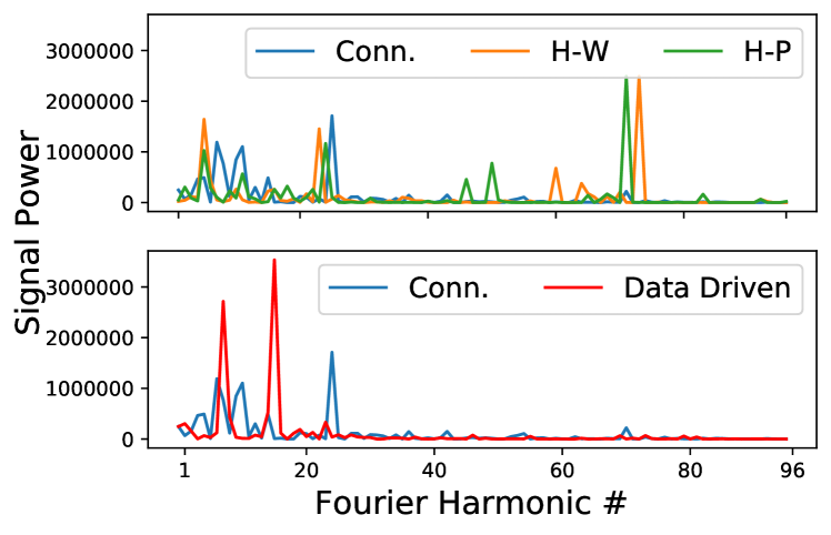
Figure 6: Total signal power of head loss at each junction in the graph Fourier domain ($0^{th}$ harmonic omitted for scaling), using different weighted network models. Top: Conn.-unweighted network using only connectivity, H-W-weights set to the inverse of the Hazen-Williams coefficients, H-P-weights set to the inverse of the Hagen-Poiseuille coefficients. None of the weighted networks produces especially low-pass or sparse graph signals. Bottom: Conn.-unweighted network using only connectivity, Data Driven-a data-driven approach designed to assign edge weights that produce low-pass characteristics.

VI Conclusion

In conclusion, we have demonstrated the importance of understanding GSP model assumptions in the context of infrastructure resilience applications. We emphasize that this work should not be interpreted as a definitive approach on the chosen techniques, rather it should be interpreted more pedagogically, as a case study analysis in a particular choice of GFT and signal model, similar to any analysis that must be performed in any practical, real-world application of these techniques. We found that system size and distributed generation capability were reasonably strong correlates to relevant GSP metrics and ultimately performance of considered GSP techniques. Thus, we note that the variability introduced by distributed generation (e.g., renewables) in relatively small networks may limit GSP techniques in micro-grid applications, and in any event should be analyzed carefully to make sure the graph signals meet the required assumptions.

Despite the observed correlations, there does appear to be considerable variation in both the metrics and performance for infrastructure systems of similar size and scope, pointing to a need for further analysis. Other than system size and distributed generation capability, we did not identify any particular characteristics of the networks that generated such variation in the metrics and results, even among networks of similar size. There are many operational and graph-centric metrics that can be explored [9, 10, 11, 12] to seek further insight, which we leave as future work. Similarly, given the usage of graph-theoretic metrics in resilience analysis of infrastructure, we conjecture that GSP-motivated metrics such as TV can provide relevant metrics that capture the state of the system over time, in a way that static network metrics cannot.

Beyond the AC power-flow derived graph model and $\bm{L}^{(|u|)}$-based GFT used here, additional combinations of graph models (such as those discussed in Sec. IV) and GFT s may be more effective for specific combinations of system and application. The results of Sec. V indicate that data-driven approaches may be able to leverage graphical structure to produce GFT s that induce desirable signal structure, and this generates additional options. Understanding how the choice of graph model and GFT impacts performance of a given GSP technique on a given system is an open question that should be studied to motivate new techniques as well as reduce future implementation and development efforts in real-world systems.

References

- [1] M. Shinozuka, “Resilience of integrated power and water system,” Seismic Evaluation and Retrofit of Life time Systems, pp. 65–86, 2004.
- [2] A. Boin and A. McConnell, “Preparing for critical infrastructure breakdowns: the limits of crisis management and the need for resilience,” Journal of Contingencies and Crisis Management, vol. 15, no. 1, pp. 50–59, 2007.
- [3] L. Duenas-Osorio and S. M. Vemuru, “Cascading failures in complex infrastructure systems,” Structural Safety, vol. 31, pp. 157–167, 2009.
- [4] M. Rudner, “Cyber-threats to critical national infrastructure: An intelligence challenge,” International Journal of Intelligence and CounterIntelligence, vol. 26, no. 3, pp. 453–481, 2013.
- [5] Y. Wang, C. Chen, J. Wang, and R. Baldick, “Research on resilience of power systems under natural disasters—a review,” IEEE Transactions on Power Systems, vol. 31, no. 2, pp. 1604–1613, 2015.
- [6] E. Hollnagel, D. D. Woods, and N. Leveson, Resilience engineering: Concepts and precepts. Ashgate Publishing, Ltd., 2006.
- [7] A. M. Madni and S. Jackson, “Towards a conceptual framework for resilience engineering,” IEEE Systems Journal, vol. 3, no. 2, pp. 181–191, 2009.
- [8] R. Patriarca, J. Bergström, G. Di Gravio, and F. Costantino, “Resilience engineering: Current status of the research and future challenges,” Safety Science, vol. 102, pp. 79–100, 2018.
- [9] Å. J. Holmgren, “Using graph models to analyze the vulnerability of electric power networks,” Risk Analysis, vol. 26, pp. 955–969, 2006.
- [10] G. A. Pagani and M. Aiello, “The power grid as a complex network: a survey,” Physica A: Statistical Mechanics and its Applications, vol. 392, no. 11, pp. 2688–2700, 2013.
- [11] A. Pagani, F. Meng, G. Fu, M. Musolesi, and W. Guo, “Quantifying resilience via multiscale feedback loops in water distribution networks,” Journal of Water Resources Planning and Management, vol. 146, no. 6, p. 04020039, 2020.
- [12] A. Pagano, C. Sweetapple, R. Farmani, R. Giordano, and D. Butler, “Water distribution networks resilience analysis: A comparison between graph theory-based approaches and global resilience analysis,” Water Resources Management, vol. 33, no. 8, pp. 2925–2940, 2019.
- [13] F. R. Chung and F. C. Graham, Spectral graph theory. American Mathematical Soc., 1997, no. 92.
- [14] M. Puschel and J. M. Moura, “Algebraic signal processing theory: Foundation and 1-d time,” IEEE Transactions on Signal Processing, vol. 56, no. 8, pp. 3572–3585, 2008.
- [15] D. Shuman, S. Narang, P. Frossard, A. Ortega, and P. Vandergheynst, “The emerging field of signal processing on graphs: Extending high-dimensional data analysis to networks and other irregular domains,” IEEE Signal Processing Magazine, vol. 3, no. 30, pp. 83–98, 2013.
- [16] A. Sandryhaila and J. M. Moura, “Discrete signal processing on graphs,” IEEE Transactions on Signal Processing, vol. 61, no. 7, pp. 1644–1656, 2013.
- [17] S. Chen, Y. Yang, C. Faloutsos, and J. Kovacevic, “Monitoring manhattan’s traffic at 5 intersections?” in 2016 IEEE Global Conference on Signal and Information Processing (GlobalSIP). IEEE, 2016, pp. 1270–1274.
- [18] M. Jamei, R. Ramakrishna, T. Tesfay, R. Gentz, C. Roberts, A. Scaglione, and S. Peisert, “Phasor measurement units optimal placement and performance limits for fault localization,” IEEE Journal on Selected Areas in Communications, vol. 38, no. 1, pp. 180–192, 2019.
- [19] Z. Wei, A. Pagani, and W. Guo, “Monitoring networked infrastructure with minimum data via sequential graph fourier transforms,” in 2019 IEEE International Smart Cities Conference (ISC2). IEEE, 2019, pp. 703–708.
- [20] R. Ramakrishna and A. Scaglione, “Detection of false data injection attack using graph signal processing for the power grid,” in 2019 IEEE Global Conference on Signal and Information Processing (GlobalSIP). IEEE, 2019, pp. 1–5.
- [21] E. Drayer and T. Routtenberg, “Detection of false data injection attacks in smart grids based on graph signal processing,” IEEE Systems Journal, 2019.
- [22] I. Jabłoński, “Graph signal processing in applications to sensor networks, smart grids, and smart cities,” IEEE Sensors Journal, vol. 17, no. 23, pp. 7659–7666, 2017.
- [23] M. A. Hasnat and M. Rahnamay-Naeini, “Detection and locating cyber and physical stresses in smart grids using graph signal processing,” arXiv preprint arXiv:2006.06095, 2020.
- [24] X. Zhu and M. Rabbat, “Approximating signals supported on graphs,” in 2012 IEEE International Conference on Acoustics, Speech and Signal Processing (ICASSP). IEEE, 2012, pp. 3921–3924.
- [25] S. Chen, A. Sandryhaila, J. M. Moura, and J. Kovačević, “Signal recovery on graphs: Variation minimization,” IEEE Transactions on Signal Processing, vol. 63, no. 17, pp. 4609–4624, 2015.
- [26] L. Stankovic, D. P. Mandic, M. Dakovic, I. Kisil, E. Sejdic, and A. G. Constantinides, “Understanding the basis of graph signal processing via an intuitive example-driven approach [lecture notes],” IEEE Signal Processing Magazine, vol. 36, no. 6, pp. 133–145, 2019.
- [27] R. Shafipour, A. Khodabakhsh, G. Mateos, and E. Nikolova, “A directed graph fourier transform with spread frequency components,” IEEE Transactions on Signal Processing, vol. 67, no. 4, pp. 946–960, 2018.
- [28] K. Schultz and M. Villafañe Delgado, “Graph signal processing of indefinite and complex graphs using directed variation,” arXiv preprint arXiv:2003.00621, 2020.
- [29] F. Chung, “Laplacians and the cheeger inequality for directed graphs,” Annals of Combinatorics, vol. 9, no. 1, pp. 1–19, 2005.
- [30] L. Liu, M. Esmalifalak, Q. Ding, V. A. Emesih, and Z. Han, “Detecting false data injection attacks on power grid by sparse optimization,” IEEE Transactions on Smart Grid, vol. 5, no. 2, pp. 612–621, 2014.
- [31] J. Valenzuela, J. Wang, and N. Bissinger, “Real-time intrusion detection in power system operations,” IEEE Transactions on Power Systems, vol. 28, no. 2, pp. 1052–1062, 2012.
- [32] R. D. Zimmerman, C. E. Murillo-Sánchez, and R. J. Thomas, “MATPOWER: Steady-state operations, planning, and analysis tools for power systems research and education,” IEEE Transactions on Power Systems, vol. 26, no. 1, pp. 12–19, 2010.
- [33] J. L. Myers, A. Well, and R. F. Lorch, Research design and statistical analysis. Routledge, 2010.
- [34] Z. Wei, A. Pagani, G. Fu, I. Guymer, W. Chen, J. A. McCann, and W. Guo, “Optimal sampling of water distribution network dynamics using graph fourier transform,” IEEE Transactions on Network Science and Engineering, 2019.
- [35] K. Klise, R. Murray, and T. Haxton, “An overview of the water network tool for resilience (wntr),” in WDSA/CCWI Joint Conference Proceedings, vol. 1, 2018.
- [36] L. A. Rossman et al., “Epanet 2: users manual,” 2000.