[1,2]Kyle E.Fitch \Author[3]ChaoxunHang \Author[1]AhmadTalaei \Author[1]Timothy J.Garrett
1]Department of Atmospheric Sciences, University of Utah, Salt Lake City, 84112, USA 2]Department of Engineering Physics, Air Force Institute of Technology, Wright-Patterson Air Force Base, Ohio, 45433, USA 3]Department of Civil Engineering, Monash University, Clayton, 3168, Australia
Kyle Fitch (kyle.fitch@us.af.mil)
Numerical simulations and Arctic observations of surface wind effects on Multi-Angle Snowflake Camera measurements
Abstract
Ground-based measurements of frozen precipitation are heavily influenced by interactions of surface winds with gauge-shield geometry. The Multi-Angle Snowflake Camera (MASC), which photographs hydrometeors in free-fall from three different angles while simultaneously measuring their fall speed, has been used in the field at multiple mid-latitude and polar locations both with and without wind shielding. Here we show results of computational fluid dynamics (CFD) simulations of the airflow and corresponding particle trajectories around the unshielded MASC and compare these results to Arctic field observations with and without a Belfort double Alter shield. Simulations in the absence of a wind shield show a separation of flow at the upstream side of the instrument, with an upward velocity component just above the aperture, which decreases the mean particle fall speed by 55%(74%) for a wind speed of (). MASC-measured fall speeds compare well with Ka-band Atmospheric Radiation Measurement (ARM) Zenith Radar (KAZR) mean Doppler velocities only when winds are light () and the MASC is shielded. MASC-measured fall speeds that do not match KAZR measured velocities tend to fall below a threshold value that increases approximately linearly with wind speed but is generally . For those events with wind speeds , hydrometeors fall with an orientation angle mode of from the horizontal plane, and large, low-density aggregates are as much as five times more likely to be observed. We conclude that accurate MASC observations of the microphysical, orientation, and fall speed characteristics of snow particles require shielding by a double wind fence and restriction of analysis to events where winds are light (). Hydrometeors do not generally fall in still air, so adjustments to these properties’ distributions within natural turbulence remain to be determined.
Accurate measurement of snowfall is of importance to a wide range of scientific and public interests, including weather and climate prediction and monitoring (Yang et al., 2005; Rasmussen et al., 2012; Thériault et al., 2015; Mekis et al., 2018), hydrological cycles (Yang et al., 2005; Rasmussen et al., 2012; Thériault et al., 2012; Mekis et al., 2018), ecosystem research (Rasmussen et al., 2012), snowpack monitoring and disaster management (Thériault et al., 2015; Mekis et al., 2018), transportation (Rasmussen et al., 2001; Thériault et al., 2012, 2015), agriculture (Mekis et al., 2018), and resource management (Thériault et al., 2015; Mekis et al., 2018).
A persistent limitation of these studies is that catch-style precipitation gauges are prone to large uncertainties, especially when measuring snowfall in high winds – a bias referred to as “under-catch" (Groisman et al., 1991; Groisman and Legates, 1994; Goodison et al., 1998; Rasmussen et al., 2001; Yang et al., 2005). A common remedy is to apply a correction based primarily on wind speed (Yang et al., 1993; Rasmussen et al., 2001, 2012; Wolff et al., 2015), although hydrometeor type (Thériault et al., 2012) and a dynamic drag coefficient (Colli et al., 2015) may also be considered. The correction is calculated by measuring the collection efficiency for a particular gauge or gauge-shield geometry, where collection efficiency is defined as the ratio of the gauge-measured precipitation rate to the best-estimate rate (Thériault et al., 2012). The Double Fence Intercomparison Reference (DFIR) is the standard reference, as determined by the World Meteorological Organization (WMO; Goodison et al., 1998); however, the DFIR has its own uncertainties which can lead to underestimation (Yang et al., 1993) or even overestimation (Thériault et al., 2015) of snowfall rates.
Surface-based measurements of solid precipitation fall speed (Garrett and Yuter, 2014), fall orientation (Garrett et al., 2015; Jiang et al., 2019), and size distributions (Thériault et al., 2012) are all very sensitive to wind speed, with fall speed and size distribution having a strong influence on precipitation gauge collection efficiency (Thériault et al., 2012, 2015). Accurate measurement of solid precipitation characteristics is important for constraining the densities and size distributions used in bulk microphysical parameterizations (e.g., Thompson et al., 2008; Morrison and Milbrandt, 2015). These parameters strongly influence bulk fall speed, highlighted by the Intergovernmental Panel on Climate Change (IPCC) as a critical factor for determining climate sensitivity (Flato et al., 2013). Likewise, knowledge of preferential hydrometeor orientation angles leads to the improved inference of hydrometeor shapes from backscattered polarimetric radar intensities (Vivekanandan et al., 1991, 1994; Matrosov et al., 2005; Matrosov, 2015), and these shapes combine with density to determine hydrometeor fall speeds (Böhm, 1989).
Past studies have typically combined airflow modeling and field observations to understand better the measurement error induced by winds and gauge geometry. Computational fluid dynamics (CFD) calculations characterize the wind velocity field and its interaction with various stationary objects in turbulent flows (Moat et al., 2006; Dehbi, 2008; Ferrari et al., 2017). Thériault et al. (2012) combined field observations and CFD simulations to better understand the scatter in collection efficiency as a function of wind speed for a Geonor, Inc. precipitation gauge located in a single Alter shield. Findings suggested that in addition to wind speed, the hydrometeor collection efficiency is a function of both hydrometeor type and size distribution. For example, hydrometeors such as graupel, with a relatively large density-to-surface-area ratio, fall faster and are collected more efficiently than large, low-density, aggregate-type hydrometeors. Additionally, Colli et al. (2016a, b) compared shielded and unshielded gauge configurations using both time-averaged and time-dependent CFD simulations and found that a single Alter shield was effective in reducing the magnitude of turbulent flow above the gauge aperture. However, upwind shield deflector fins still produced turbulence that propagated into the collection area and generally reduced the collection efficiency.
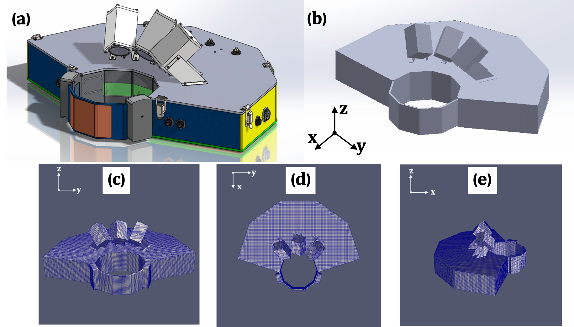
One instrument that has received increased attention, but whose sampling characteristics have yet to be characterized in detail, is the Multi-Angle Snowflake Camera (MASC; Garrett et al., 2012). The MASC system has overall dimensions of 43.5 cm x 58 cm x 21.5 cm (Stuefer and Bailey, 2016) and observes particles falling into a ring-shaped collection area. The ring houses three cameras focused on a point at the ring center 10 cm away, with each camera separated by 36\unit^∘ (Garrett et al., 2012). A coupled system of directly opposing near-infrared emitters and detectors, vertically separated by 32 \unitmm, detect falling hydrometeors larger than approximately 0.1 \unitmm in maximum dimension. This triggers the cameras and three high-powered LEDs located directly above (Garrett and Yuter, 2014). The time between triggers of the upper and lower emitter-detector pairs yields a fall speed. High-resolution images are captured at an exposure time of 1/25,000th of a second, sufficient to capture a vertical resolution of 40 \unitμm in a hydrometeor falling at 1 \unitm s^-1 (Garrett et al., 2012).
The MASC system has helped to advance precipitation measurement by automating simultaneous high-resolution photography and fall speed measurement of falling hydrometeors from multiple angles, removing the need for tedious manual collection. Variables derived from the high-resolution images include those describing a hydrometeor’s size, shape, fall orientation, and approximate riming degree (Garrett et al., 2012; Garrett and Yuter, 2014; Garrett et al., 2015). As these hydrometeor properties are crucial for accurate numerical modeling and microwave scattering calculations, the MASC has been used at various polar and mid-latitude locations to constrain microphysical characteristics (Garrett et al., 2012; Garrett and Yuter, 2014; Garrett et al., 2015; Grazioli et al., 2017; Kim et al., 2018; Dunnavan et al., 2019; Jiang et al., 2019; Kim et al., 2019; Vignon et al., 2019), improve radar-based estimates of snowfall rates (Gergely and Garrett, 2016; Cooper et al., 2017; Schirle et al., 2019), automatically classify hydrometeors (Praz et al., 2017; Besic et al., 2018; Hicks and Notaroš, 2019; Leinonen and Berne, 2020; Schaer et al., 2020), reconstruct particle shapes (Notaroš et al., 2016; Kleinkort et al., 2017) and size distributions (Cooper et al., 2017; Huang et al., 2017; Schirle et al., 2019), and as ground truth comparisons for radar measurements (Bringi et al., 2017; Gergely et al., 2017; Matrosov et al., 2017; Kennedy et al., 2018; Oue et al., 2018; Matrosov et al., 2019). Unlike more common precipitation gauges, the wind velocity field in the proximity of the MASC has not been simulated for various surface winds speeds, directions, or turbulence kinetic energies (TKE).
Studies of hydrometeor behaviors using the MASC have shown, somewhat surprisingly, that frozen hydrometeor fall speeds are only weakly dependent on their size or shape, particularly under conditions of high turbulence intensity (Garrett and Yuter, 2014). Prior studies had shown a much stronger dependence but had theoretically assumed or experimentally arranged for falling hydrometeors to settle in still air (Locatelli and Hobbs, 1974; Böhm, 1989). MASC measurements led to a hypothesis that snow "swirls" in turbulent air in a manner that spreads particle fall speeds to both higher and lower values (Garrett and Yuter, 2014) – an effect shown in prior work to be non-negligible in turbulent flows (Nielsen, 2007). While the fact that snowflakes can just as readily move upwards as downwards is easily verified by any casual observations of a winter storm, it has remained unclear the extent to which the measurements of snowflake fall speed obtained by the MASC have been reflective of reality rather than some artifact of interactions of surrounding winds with the instrument body.
In this study, we describe CFD simulations of hydrometeor-instrument interactions with specific application to the MASC. We compare these simulations to field observations of hydrometeor characteristics from a MASC located in the Arctic. The goal of this study is to better understand and characterize the influence of ambient wind speeds on MASC measurements of hydrometeor fall speed, fall orientation, and size distribution for both wind-shielded and unshielded configurations.
1 CFD simulations
To explore how ambient winds affect MASC measurements of fall speed, we use the OpenFOAM 4.1 tool (Jasak et al., 2007) for CFD calculations of falling particles and winds interacting with the MASC body. OpenFOAM is an open-source CFD toolbox based on C++ libraries and codes designed to solve complex flow dynamics problems (Jasak et al., 2007; Chen et al., 2014; Greenshields, 2015). The solver uses the factorized finite volume method (FVM) with the Semi-Implicit Method for Pressure Linked Equations (SIMPLE) algorithm (Caretto et al., 1973) to solve the Navier–Stokes equations. The – Shear Stress Transport (SST) model is utilized in this study to solve the turbulence closure problem due to its capability to capture the flow separation near objects through the viscous sub-layer, without additional wall functions (Menter, 1993). We combine the incompressible, robust simpleFOAM solver for steady incompressible turbulent flows (Balogh et al., 2012; Higuera et al., 2014) with the solidParticle and solidParticleCloud classes to study the motions of particles (Iudiciani, 2009).
To study particle-air interactions, the first step is to determine the two-phase flow type. The ratio between the average inter-particle distance and the particle diameter is estimated. Provided the ratio is , the flow can be treated as a dilute dispersed system, and one-way coupling – wherein the particles do not collide with each other and also do not affect the flow field – can be assumed (Elghobashi, 1994). The OpenFOAM blockMesh and snappyHexMesh tools are applied here to generate a mesh around the complex physical geometry of the MASC instrument (Gisen, 2014). The snappyHexMesh utility automatically generates 3D meshes containing hexahedra and split-hexahedra efficiently. Figure 1(c–e) shows the MASC mesh for different viewing angles. Spatial and temporal parameters are provided in Table 1.
| \tophline\middlehlineDomain Dimensions | ||
|---|---|---|
| Width (x–dir) | 4 \unitm | |
| Transverse thickness (y–dir) | 4 \unitm | |
| Height (z–dir) | 10 \unitm | |
| Grid (x y z) | 16 16 40 | |
| Particle properties | ||
| Number of particles | 400 | |
| Diameter () | 2 \unitmm | |
| Density () | 50 \unitkg m^-3 | |
| Fluid properties (at 0 ∘C) | ||
| Viscosity () | 1.34 \unitm^2 s^-1 | |
| Density () | 1.284 \unitkg m^-3 | |
| \bottomhline |
For the simulation of hydrometeors in the atmosphere, we track spherical particles of mass , diameter , and area within a Lagrangian framework, where the Eulerian fluid velocity field is interpolated from nearby grid points at the position of the particle to compute the instantaneous particle drag. The particle velocity is calculated at each time step by assuming that the particle’s Reynolds number is greater than unity, which gives a reduced form of the Maxey–Riley equation of motion (Maxey and Riley, 1983):
| (1) |
where the drag coefficient is a function of the relative Reynolds number , is the fluid density, and is the gravitational constant. Particles measured with the MASC had a median of 108, with of the values in the range of .
In simulations of the response of the particles to horizontal winds in the vicinity of the MASC, the particles are evenly distributed on a 2020 grid with 1 \unitmm spacing in the x–direction and 2 \unitmm spacing in the y–direction. The particles fall downward at an initial velocity of from a height of above the MASC in the direction under the force of gravity, reaching an average terminal velocity of well before encountering flows perturbed by the MASC.
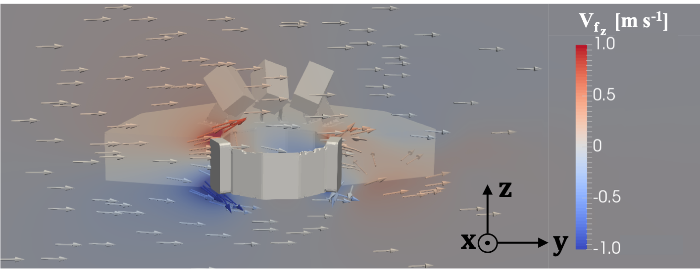
Figure 2 shows interactions of a horizontal flow in the +y direction of 1 \unitm s^-1 with the MASC body. There is a clear separation of flow on the upstream side of the aperture, a relatively large upward component above the aperture, and a smaller downward component within the aperture.
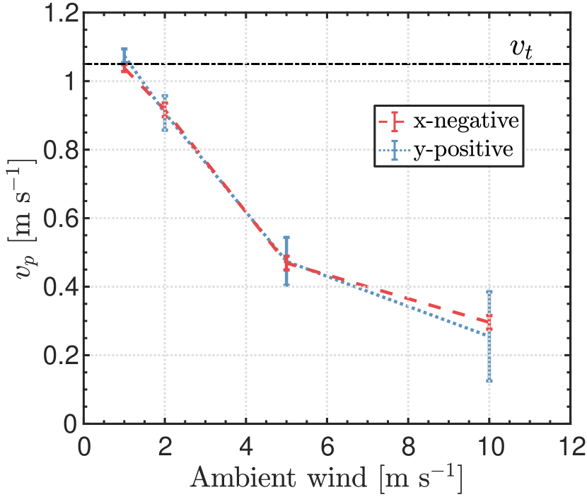
The response of particles to these perturbations for horizontal winds in both the and directions is shown in Fig. 3. There is low sensitivity to wind direction, but the mean particle fall speed within the MASC aperture decreases from to as the ambient wind speed increases from 1 to (Table 2).
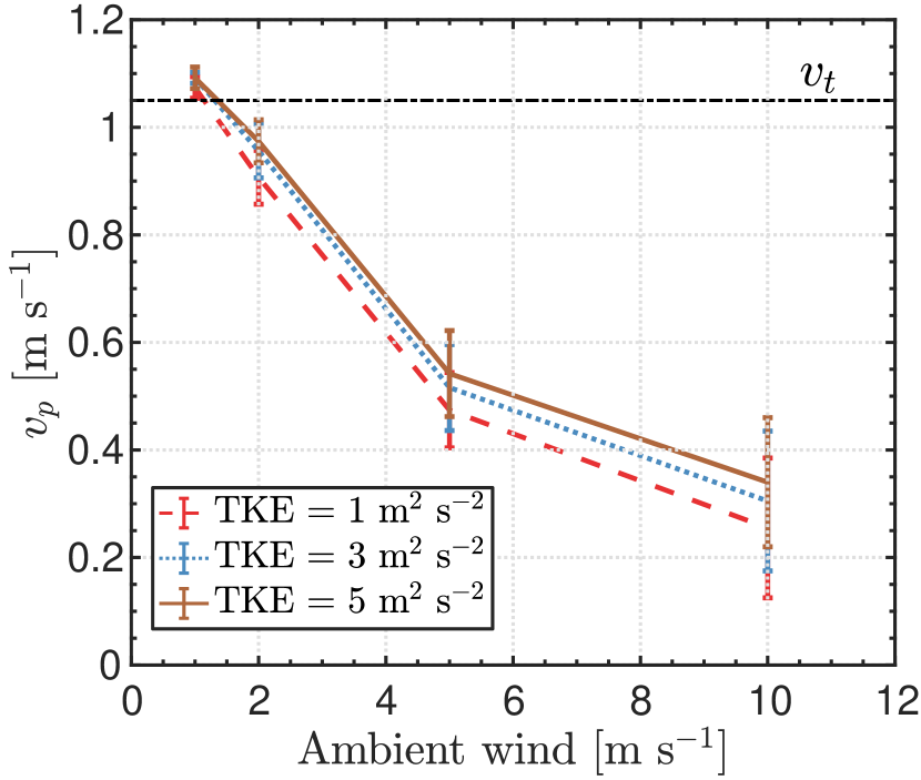
The influence of ambient turbulent intensity expressed as was calculated for , 3, and 5 \unitm^2 s^-2, where the perturbation velocity is the difference between the instantaneous and average velocities of the atmospheric flow. These TKE values are used as initial conditions in the – closure model, which determines the shear stress, which in turn is used in the momentum budget equation. Figure 4 shows that for a wind speed of , the mean particle fall speed is 24% lower for an initial value of than it is for (Table 2).
| \tophlineAmbient wind | ||||
|---|---|---|---|---|
| \middlehlineWind Direction | ||||
| x-negative | 1.07 \unitm s^-1 | 0.92 \unitm s^-1 | 0.47 \unitm s^-1 | 0.30 \unitm s^-1 |
| y-positive | 1.04 \unitm s^-1 | 0.91 \unitm s^-1 | 0.47 \unitm s^-1 | 0.26 \unitm s^-1 |
| \middlehlineTKE | ||||
| 1 \unitm^2 s^-2 | 1.07 \unitm s^-1 | 0.91 \unitm s^-1 | 0.47 \unitm s^-1 | 0.26 \unitm s^-1 |
| 3 \unitm^2 s^-2 | 1.09 \unitm s^-1 | 0.96 \unitm s^-1 | 0.52 \unitm s^-1 | 0.31 \unitm s^-1 |
| 5 \unitm^2 s^-2 | 1.09 \unitm s^-1 | 0.98 \unitm s^-1 | 0.54 \unitm s^-1 | 0.34 \unitm s^-1 |
| \bottomhline |
2 Hydrometeor observations
2.1 Methods
Processing of MASC imagery consists of distinguishing foreground pixels from background to define the region of interest (ROI) and then fitting the ROI with a bounding ellipse (Shkurko et al., 2018). The ellipse’s major axis is defined as the maximum dimension for each image. The absolute value of the angle between and the local horizontal plane is the orientation angle (Garrett et al., 2012; Garrett and Yuter, 2014; Garrett et al., 2015; Shkurko et al., 2018). A complexity parameter is used to distinguished riming classes (Garrett and Yuter, 2014). Here we use to identify heavily rimed graupel, for moderate riming, and indicates sparsely-rimed aggregates. We note that a value of 1.75 was used to distinguish moderately rimed particles from aggregates for Utah snow measurements in Garrett and Yuter (2014), with the observation that the value is subjectively determined by visual inspection of hydrometeor images and varies with location. Mean values of fall speed , , , and from all three images are used for each particle.
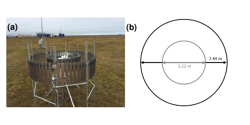
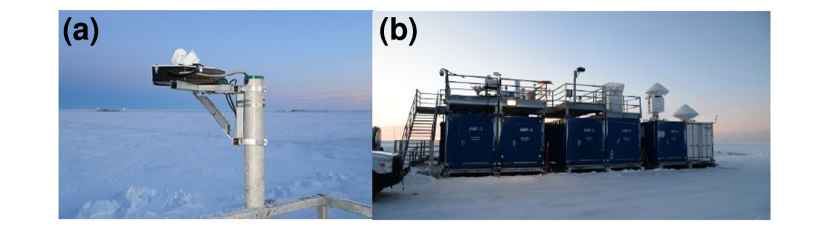
A MASC was installed at the Department of Energy’s Third Atmospheric Radiation Measurement (ARM) Mobile Facility (AMF3), Oliktok Point, Alaska, in February 2015. The initial deployment was atop a group of shipping containers with no wind shield (Fig. 5). On 22 August 2016, the MASC was relocated to ground level and placed inside of a Belfort Model 36001 Double Alter Wind Shield (Fig. 6). The central camera was pointed in the east-northeasterly direction (Jiang et al., 2019), with surface wind observations showing this to be the predominant wind direction for the present study. The inner(outer) fence of the shield is 1.22(2.44) in diameter, with 32(64) deflector fins that are each 46(61) in length. Observations used here include both unshielded and shielded configurations, spanning a 33-month period from 29 November 2015 to 28 August 2018 (ARM Climate Research Facility, 2014). Raw data and images were processed with a local University of Utah processing suite called mascpy (The Hive: University of Utah Research Data Repository, 2020a, b), similar to that described in Shkurko et al. (2018).
To complement MASC observations and characterize the influence of ambient wind speed on MASC measurements, surface wind measurements from a traditional meteorological ground suite (Ritsche, 2011; ARM Climate Research Facility, 2013) were matched to MASC hydrometeors by calculating a mean wind speed for the 1 minute period leading up to the observation time corresponding to each hydrometeor. In addition to the quality control checks listed in Shkurko et al. (2018), a surface temperature threshold of was used to exclude liquid hydrometeors, which are occasionally misidentified by the mascpy algorithm.
For a ground truth hydrometeor fall speed, mean Doppler velocity was calculated from the volume of scattering hydrometeors detected by a co-located Ka-band ARM Zenith-pointing Radar (KAZR). At a vertical resolution of 30 m, the KAZR produces measurements of the first three moments of the Doppler spectrum: reflectivity, mean Doppler velocity, and spectrum width (Widener et al., 2012; Oue et al., 2018). The Doppler velocity signal has a resolution of 0.05 \unitm s^-1 (Oue et al., 2018) and consists of both larger particle fall speeds and the vertical air motions traced by smaller particles (Shupe et al., 2008). Using only Doppler velocity measurements originating from below cloud base, we isolate the signal of the larger, precipitation-sized hydrometeors, while acknowledging the relatively small bias of Doppler broadening from turbulence and wind shear (Shupe et al., 2008). Both mean Doppler velocity and cloud base height were retrieved from the ARM’s KAZR Active Remote Sensing of CLouds (ARSCL) Value-Added Product (ARM Climate Research Facility, 2015; Clothiaux et al., 2000).
Results are presented here in the form of probability density function (PDF) estimates, calculated by normalizing the frequency of each histogram bin of width (equally spaced bins), such that . Here is the total number of observations, and is the variable of interest. The resulting PDF estimates were adjusted using a Gaussian kernel smoothing function. For distributions of , the exponential slope parameter is computed using a linear least squares regression from the peak of the log-linear distribution through the tail.
2.2 Observations of fall speed
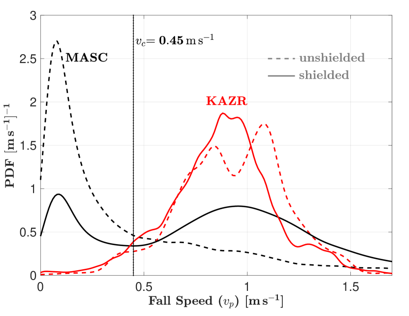
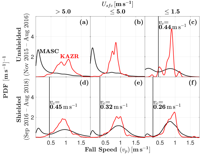
Distributions of MASC-measured particle fall speed , both with and without a wind shield, are compared to coincident measurements from the KAZR in Fig. 7. The KAZR-measured fall speed mode is , while the MASC-measured fall speed distribution has a mode of 0.08 \unitm s^-1 for both the shielded and unshielded cases. However, the shielded MASC fall speed distribution has a second mode at 0.96 \unitm s^-1, similar to the location of the KAZR mode. Notably, a low-speed mode was not observed in the KAZR measurements despite its velocity resolution of 0.05 \unitm s^-1.
The shielded MASC fall speed distribution deviates substantially from the corresponding KAZR distribution for fall speeds below . This is the location of the local minimum separating the two modes of the shielded MASC fall speed distribution and is defined from here on as the cutoff fall speed : the fall speed below which MASC measurements are assumed to be erroneous. The fall speed distribution can therefore be divided into two parts: and .
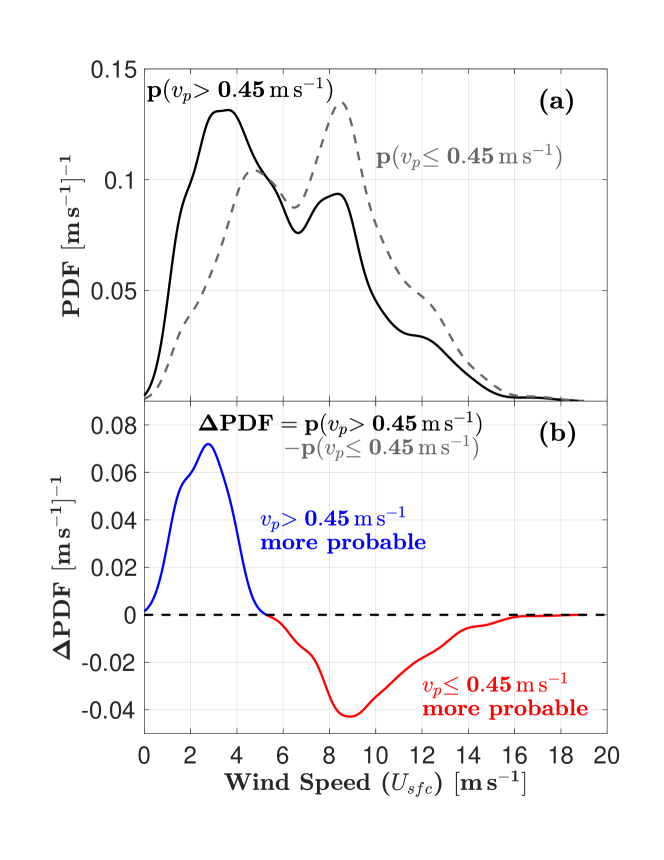
To examine the influence of surface wind speeds on MASC fall speed measurements, Fig. 8 shows PDF estimates of wind speed for the two separate parts of the shielded MASC fall speed distribution from Fig. 7. From the difference (Fig. 8(b)), it is apparent that the high-speed mode of is more likely to be observed when . This matches well with the simulated fall speeds in wind speeds of from Table 2 and Figs. 3 and 4, although the simulation did not include a wind fence.
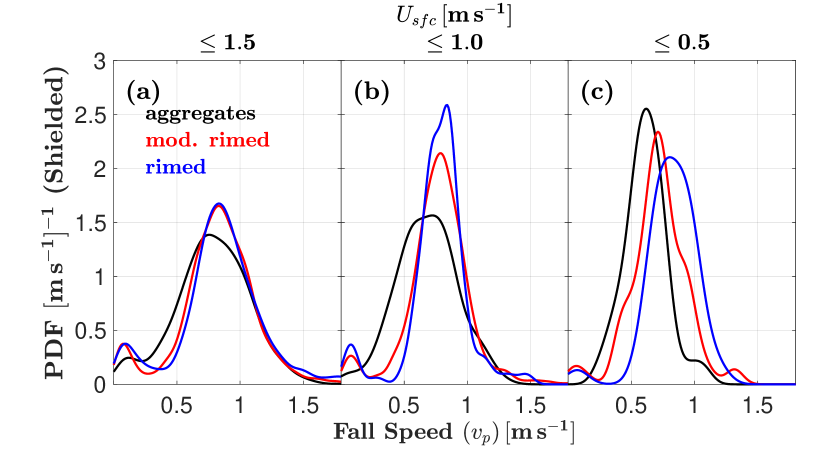
Figure 9 compares MASC and KAZR fall speed distributions as a function of , again both with and without wind shielding of the MASC. Qualitatively, the agreement between the MASC and KAZR distributions is maximized for shielded MASC measurements with light winds (), where only 7% of measured fall speeds are lower than the threshold of (Fig. 9(f)). When separated by riming class, shielded MASC fall speed distributions show discernible differences only for the lightest winds. This is most apparent for (Fig. 10(c)), where the most heavily rimed particles () tend to exhibit the highest fall speeds. Particle counts corresponding to Figs. 9 and 10 are listed in Table 3.
| \tophline | |||||
| Category | |||||
| \middlehlineNo Wind Shield | 2,249 | 5,097 | 460 | 167 | 32 |
| Aggregates | 176 (8%) | 1,522 (30%) | 67 (15%) | 15 (9%) | 5 (16%) |
| Moderately Rimed | 1,209 (54%) | 2,891 (57%) | 315 (68%) | 115 (69%) | 14 (44%) |
| Rimed | 864 (38%) | 684 (13%) | 78 (17%) | 37 (22%) | 13 (41%) |
| \middlehlineWind Shield | 85,151 | 58,939 | 5,730 | 1,372 | 161 |
| Aggregates | 15,320 (18%) | 11,304 (19%) | 1,299 (23%) | 302 (22%) | 41 (25%) |
| Moderately Rimed | 47,147 (55%) | 35,820 (61%) | 3,477 (61%) | 855 (62%) | 86 (53%) |
| Rimed | 22,684 (27%) | 11,815 (20%) | 954 (17%) | 215 (16%) | 34 (21%) |
| \bottomhline |
2.3 Observations of orientation, maximum dimension, and riming degree
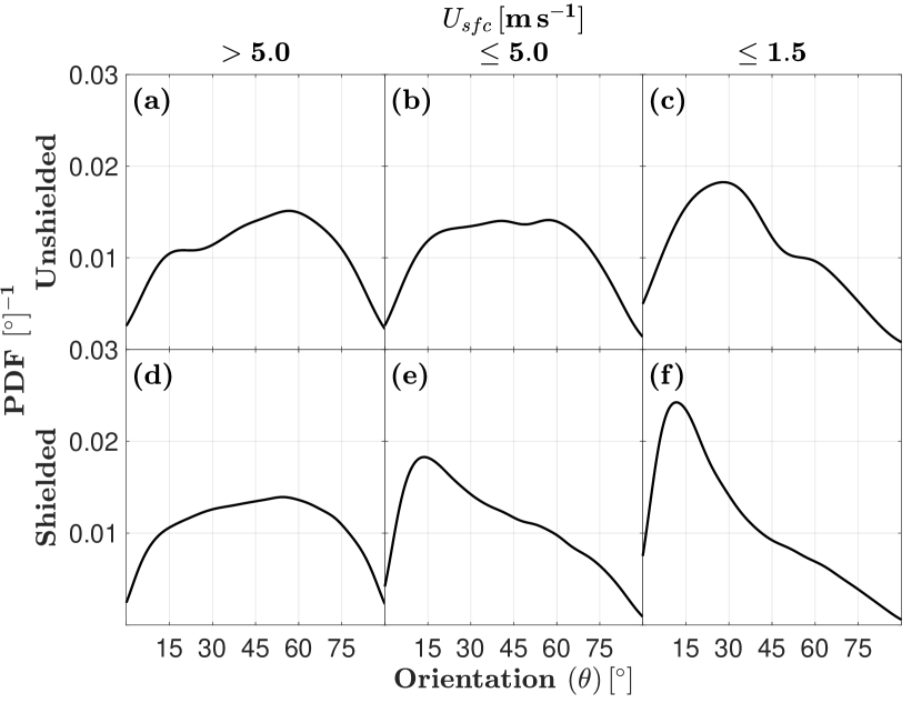
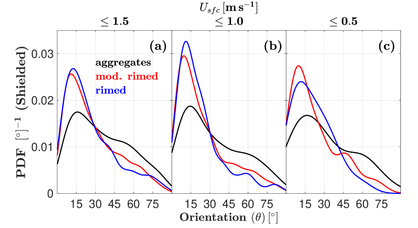
Distributions of unshielded MASC-measured orientation angles tend to favor high angles in high winds (, Fig. 11(a)), where the mode is , but this shifts to for the lightest winds (, Fig. 11(c)). Shielded measurements tend towards even lower angles in the lightest winds, with a mode of for (Fig. 11(f)). These results suggest that these solid hydrometeors tend to fall with their maximum dimensions nearly aligned with the horizontal plane when left undisturbed by surface winds. When separated by riming class for the lightest winds (), shielded MASC orientation angles tend to be larger (i.e., more vertical) for sparsely-rimed aggregates (Fig. 12).
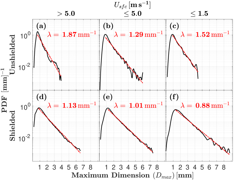
To examine surface wind influence on hydrometeor sizes observed by the MASC, distributions of and corresponding values are shown in Fig. 13. The slope parameter is smallest when the MASC is shielded and surface winds are very light (, Fig. 13(f)), and largest for unshielded observations in high winds (, Fig. 13(a)). This suggests that the largest hydrometeors are less likely to be captured by the MASC in strong winds, and even less likely without shielding. When these wind-shielded distributions are separated into riming degree classes (Fig. 14), aggregates exhibit a 26% percent decrease in , from 0.88 to 0.65 , when comparing high winds () to low winds (). For a size distribution with the form , where is the concentration of particles with sizes between and , this decrease in corresponds to a number concentration that is 5 times higher for aggregates with . In contrast, moderately and heavily rimed hydrometeors only exhibit a decrease of 13% and 11%, respectively, when comparing high- and low-wind measurements.
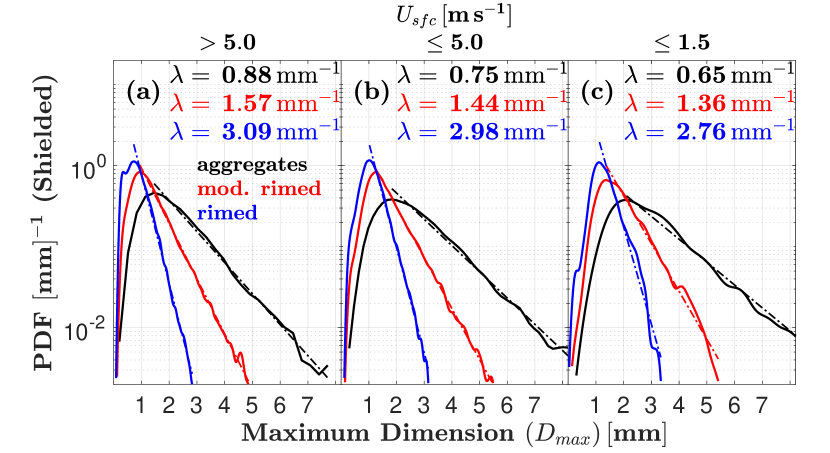
The observation that measured concentrations of larger aggregates are relatively sensitive to surface winds compared to more heavily rimed particle types suggests that the frequency distribution of riming classes observed by the MASC might also reflect this sensitivity. Indeed, Table 3 shows that the percentage of wind-shielded aggregates reaches a maximum (25%) when wind speeds are lowest (). The opposite is true for shielded rimed hydrometeors (i.e., graupel), implying that high-density rimed particles are more likely to be observed by the MASC than large, weakly rimed aggregates in the presence of strong winds ().
3 Discussion
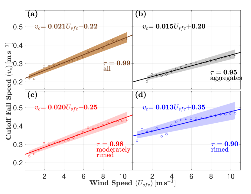
The cutoff fall speed defined in Sect. 2.2 is a potentially useful threshold for quality control of MASC fall speed measurements, and Fig. 9 suggests that for shielded MASC measurements. Least squares linear regression fits of to are plotted in Fig. 15 in increments of 0.5 \unitm s^-1. Goodness-of-fit is 0.95 or greater for all but the most heavily rimed particles, where a value of 0 indicates no relationship, and 1 indicates a perfect relationship. Data points tend to fall outside the 95% confidence interval for the most restricted wind speeds (, or for graupel), corresponding to the lowest number of observations. These fits can be used as a guide for quality control of shielded MASC measurements, where particles with fall speeds below are either omitted or corrected through extrapolation.
Larger aggregates with negligible riming tend to be more susceptible to disturbance by surface winds and associated turbulence, with more vertical orientations and lower frequency of occurrence than other riming classes. This finding supports that of Thériault et al. (2012), who found that faster-falling hydrometeors are collected more efficiently by a Geonor gauge inside a single Alter shield. Therefore particle type needs to be considered when accounting for the effect of wind speed on snow measurements. However, the collection efficiencies for all riming classes sampled in the present study are found to be highly sensitive to winds in the absence of a wind shield. This sensitivity is reduced but still apparent for all but perhaps the very lightest winds , even when located inside of a double wind fence. This is likely the result of upstream turbulence propagating into the collection area as a result of wind interacting with shield deflector fins, as suggested in Colli et al. (2016a, b).
Prior MASC observations (Garrett and Yuter, 2014) and work by Nielsen (2007) have shown that fall speed distributions are broadened in highly turbulent flows, where fall speeds are either enhanced are reduced by turbulent eddies. Considering also that the MASC observes one hydrometeor at a time, while the KAZR fall speed is the mean value from a volume of scattering hydrometeors, it is certainly possible that at least some of the measurements comprising the low-fall-speed mode of the MASC fall speed distributions are a natural result of turbulence and not caused by the interaction of surface winds with the MASC or MASC-shield configuration. However, without more direct fall speed measurements to compare with, the highest confidence in the MASC fall speed measurements is achieved by omitting measured fall speeds that fall below .
Accurate measurement of solid hydrometeor fall speed, orientation, and size distribution is critical for constraining numerical model parameterizations and remote sensing retrievals. Surface winds are known to have a strong influence on the collection of solid hydrometeors that is dependent on the specific gauge-shield configuration. Simulations of wind interactions with an unshielded MASC showed an average reduction in mean particle fall speed of 74% for winds increasing to , while TKE had only a weak, inverse effect on the reduction. In comparison with coincident KAZR observations of mean Doppler velocity, MASC measurements of fall speed were in closest agreement only when both the MASC was shielded with a double wind fence and winds were light (). For the lightest wind speeds (), shielded measurements of orientation angles decreased to a mode of , and concentrations of sparsely-rimed aggregates with increased by a factor of five. However, we showed that even in these wind-restricted and shielded cases, a fraction of MASC-measured fall speeds – those below a wind-speed-dependent cutoff fall speed that is most often – still do not match KAZR measurements. We showed that this cutoff fall speed is a function of wind speed for shielded observations and provided linear regression fits that can be used for additional quality control of MASC measurements.
Future work could include a double wind fence in the CFD simulation to see more precisely how the wind field evolves as it encounters the individual deflector fins in each portion of the fence, where these fins are allowed to move with the wind. Thériault et al. (2012) simulated the wind field for a Geonor gauge with a single Alter shield by accounting for the movement of deflector fins on the upstream side of the gauge, where fins were assigned angles with respect to the vertical that increased as a function of wind speed. Such careful simulation might improve the fidelity of wind-shield-gauge influence on snow measurements.
The intent of this work is to provide guidance for under what measurement conditions the MASC can be used to obtain accurate information about hydrometeor microphysical properties and fall speeds. However, those conditions are limited to measurements within still air. The distributions of frozen hydrometeor size, type, orientation, and fall speed in natural, turbulent air remain to be determined.
The code and data supporting this project are available at https://doi.org/10.7278/S50DQTX9K7QY. This repository includes code sufficient to replicate the observations analysis results. Raw and processed MASC data are available from the ARM data archive at https://adc.arm.gov/discovery/#/, and raw MASC data can be processed with the mascpy code located at https://doi.org/10.7278/S50DVA5JK2PD. OpenFoam v4.1 software can be downloaded at https://openfoam.org/version/4-1/.
All authors contributed to the formulation of the project. KF and TG developed the methodology and software code for observations analysis. CH developed the methodology and software implementation for the simulations, with AT advising. KF and CH wrote the article with contributions from TG and AT.
TG is co-owner and scientific advisor of Particle Flux Analytics, Inc., the company manufacturing the Multi-Angle Snowflake Camera. Otherwise, the authors declare that they have no conflict of interest.
Acknowledgements.
This work was supported by the Department of Energy Atmospheric System Research program Grant DE-SC0016282 and the National Science Foundation (NSF) Physical and Dynamic Meteorology program award number 1841870. We thank Krista Gaustad and Martin Stuefer for sharing precise dates, locations, and orientations of the instrument and wind shield.References
- ARM Climate Research Facility (2013) ARM Climate Research Facility: Surface Meteorological Instrumentation (MET), 2014-11-11 to 2018-09-09, ARM Mobile Facility (OLI) Oliktok Point, Alaska; AMF3 (M1). Compiled by M. Ritsche, J. Kyrouac, N. Hickmon and D. Holdridge. ARM Data Center: Oak Ridge, Tennessee, USA. Data set accessed 2019-10-09 at http://dx.doi.org/10.5439/1025220, 2013.
- ARM Climate Research Facility (2014) ARM Climate Research Facility: Multi-Angle Snowflake Camera (MASC), 2015-11-29 to 2018-08-28, ARM Mobile Facility (OLI) Oliktok Point, Alaska; AMF3 (M1). Compiled by B. Ermold, K. Shkurko, and M. Stuefer. ARM Data Center: Oak Ridge, Tennessee, USA. Data set accessed 2018-09-26 at http://dx.doi.org/10.5439/1234550, 2014.
- ARM Climate Research Facility (2015) ARM Climate Research Facility: Active Remote Sensing of CLouds (ARSCL) product using Ka-band ARM Zenith Radars (ARSCLKAZR1KOLLIAS), 2015-11-29 to 2018-09-10, ARM Mobile Facility (OLI) Oliktok Point, Alaska; AMF3 (M1). Compiled by Compiled by K. Johnson, T. Toto and S. Giangrande. ARM Data Center: Oak Ridge, Tennessee, USA. Data set accessed 2019-10-14 at http://dx.doi.org/10.5439/1350629, 2015.
- Balogh et al. (2012) Balogh, M., Parente, A., and Benocci, C.: RANS simulation of ABL flow over complex terrains applying an Enhanced k- model and wall function formulation: Implementation and comparison for fluent and OpenFOAM, Journal of Wind Engineering and Industrial Aerodynamics, 104, 360–368, 2012.
- Besic et al. (2018) Besic, N., Gehring, J., Praz, C., Figueras i Ventura, J., Grazioli, J., Gabella, M., Germann, U., and Berne, A.: Unraveling hydrometeor mixtures in polarimetric radar measurements, Atmospheric Measurement Techniques, 11, 4847–4866, 10.5194/amt-11-4847-2018, 2018.
- Böhm (1989) Böhm, H. P.: A general equation for the terminal fall speed of solid hydrometeors, Journal of the Atmospheric Sciences, 46, 2419–2427, 10.1175/1520-0469(1989)046%3C2419:AGEFTT%3E2.0.CO;2, 1989.
- Bringi et al. (2017) Bringi, V., Kennedy, P., Huang, G.-J., Kleinkort, C., Thurai, M., and Notaroš, B.: Dual-polarized radar and surface observations of a winter graupel shower with negative Z dr column, Journal of Applied Meteorology and Climatology, 56, 455–470, 10.1175/JAMC-D-16-0197.1, 2017.
- Caretto et al. (1973) Caretto, L., Gosman, A., Patankar, S., and Spalding, D.: Two calculation procedures for steady, three-dimensional flows with recirculation, in: Proceedings of the third international conference on numerical methods in fluid mechanics, pp. 60–68, Springer, 10.1007/BFb0112677, 1973.
- Chen et al. (2014) Chen, G., Xiong, Q., Morris, P. J., Paterson, E. G., Sergeev, A., and Wang, Y.: OpenFOAM for computational fluid dynamics, Notices of the AMS, 61, 354–363, 10.1090/noti1095, 2014.
- Clothiaux et al. (2000) Clothiaux, E. E., Ackerman, T. P., Mace, G. G., Moran, K. P., Marchand, R. T., Miller, M. A., and Martner, B. E.: Objective determination of cloud heights and radar reflectivities using a combination of active remote sensors at the ARM CART sites, Journal of Applied Meteorology, 39, 10.1175/1520-0450(2000)039%3C0645:ODOCHA%3E2.0.CO;2, 2000.
- Colli et al. (2015) Colli, M., Rasmussen, R., Thériault, J. M., Lanza, L. G., Baker, C. B., and Kochendorfer, J.: An improved trajectory model to evaluate the collection performance of snow gauges, Journal of Applied Meteorology and Climatology, 54, 1826–1836, 10.1175/JAMC-D-15-0035.1, 2015.
- Colli et al. (2016a) Colli, M., Lanza, L. G., Rasmussen, R., and Thériault, J. M.: The collection efficiency of shielded and unshielded precipitation gauges. Part I: CFD airflow modeling, Journal of Hydrometeorology, 17, 231–243, 10.1175/JHM-D-15-0010.1, 2016a.
- Colli et al. (2016b) Colli, M., Lanza, L. G., Rasmussen, R., and Thériault, J. M.: The collection efficiency of shielded and unshielded precipitation gauges. Part II: Modeling particle trajectories, Journal of Hydrometeorology, 17, 245–255, 10.1175/JHM-D-15-0011.1, 2016b.
- Cooper et al. (2017) Cooper, S. J., Wood, N. B., and L’Ecuyer, T. S.: A variational technique to estimate snowfall rate from coincident radar, snowflake, and fall-speed observations, Atmospheric Measurement Techniques (Online), 10, 10.5194/amt-10-2557-2017, 2017.
- Dehbi (2008) Dehbi, A.: A CFD model for particle dispersion in turbulent boundary layer flows, Nuclear Engineering and Design, 238, 707–715, 10.1016/j.nucengdes.2007.02.055, 2008.
- Dunnavan et al. (2019) Dunnavan, E. L., Jiang, Z., Harrington, J. Y., Verlinde, J., Fitch, K., and Garrett, T. J.: The Shape and Density Evolution of Snow Aggregates, Journal of the Atmospheric Sciences, 76, 3919–3940, 10.1175/JAS-D-19-0066.1, 2019.
- Elghobashi (1994) Elghobashi, S.: On predicting particle-laden turbulent flows, Applied Scientific Research, 52, 309–329, 10.1007/BF00936835, 1994.
- Ferrari et al. (2017) Ferrari, G., Federici, D., Schito, P., Inzoli, F., and Mereu, R.: CFD study of Savonius wind turbine: 3D model validation and parametric analysis, Renewable Energy, 105, 722–734, 10.1016/j.renene.2016.12.077, 2017.
- Flato et al. (2013) Flato, G., Marotzke, J., Abiodun, B., Braconnot, P., Chou, S., Collins, W., Cox, P., Driouech, F., Emori, S., Eyring, V., Forest, C., Gleckler, P., Guilyardi, E., Jakob, C., Kattsov, V., Reason, C., and Rummukainen, M.: Evaluation of Climate Models, book section 9, p. 820, Cambridge University Press, Cambridge, United Kingdom and New York, NY, USA, https://doi.org/10.1017/CBO9781107415324.020, URL www.climatechange2013.org, 2013.
- Garrett and Yuter (2014) Garrett, T. J. and Yuter, S. E.: Observed influence of riming, temperature, and turbulence on the fallspeed of solid precipitation, Geophysical Research Letters, 41, 6515–6522, 10.1002/2014GL061016, 2014.
- Garrett et al. (2012) Garrett, T. J., Fallgatter, C., Shkurko, K., and Howlett, D.: Fall speed measurement and high-resolution multi-angle photography of hydrometeors in free fall, Atmospheric Measurement Techniques, 5, 2625–2633, 10.5194/amt-5-2625-2012, 2012.
- Garrett et al. (2015) Garrett, T. J., Yuter, S. E., Fallgatter, C., Shkurko, K., Rhodes, S. R., and Endries, J. L.: Orientations and aspect ratios of falling snow, Geophysical Research Letters, 42, 4617–4622, 10.1002/2015GL064040, 2015.
- Gergely and Garrett (2016) Gergely, M. and Garrett, T. J.: Impact of the natural variability in snowflake diameter, aspect ratio, and orientation on modeled snowfall radar reflectivity, Journal of Geophysical Research: Atmospheres, 121, 12–236, 10.1002/2016JD025192, 2016.
- Gergely et al. (2017) Gergely, M., Cooper, S. J., and Garrett, T. J.: Using snowflake surface-area-to-volume ratio to model and interpret snowfall triple-frequency radar signatures, Atmospheric Chemistry and Physics (Online), 17, 10.5194/acp-17-12011-2017, 2017.
- Gisen (2014) Gisen, D.: Generation of a 3D mesh using snappyHexMesh featuring anisotropic refinement and near-wall layers, in: ICHE 2014. Proceedings of the 11th International Conference on Hydroscience & Engineering, pp. 983–990, 2014.
- Goodison et al. (1998) Goodison, B. E., Louie, P. Y. T., and Yang, D.: WMO Solid Precipitation Measurement Intercomparison, report WMO/TD No. 872, World Meteorological Organization, 1998.
- Grazioli et al. (2017) Grazioli, J., Genthon, C., Boudevillain, B., Duran-Alarcon, C., Del Guasta, M., Madeleine, J.-B., and Berne, A.: Measurements of precipitation in Dumont d’Urville, Adélie Land, East Antarctica, Cryosphere, 11, 1797–1811, 10.5194/tc-11-1797-2017, 2017.
- Greenshields (2015) Greenshields, C. J.: OpenFOAM User Guide, FM Global, v3.0.1, 2015.
- Groisman and Legates (1994) Groisman, P. Y. and Legates, D. R.: The accuracy of United States precipitation data, Bulletin of the American Meteorological Society, 75, 215–228, 10.1175/1520-0477(1994)075<0215:TAOUSP>2.0.CO;2, 1994.
- Groisman et al. (1991) Groisman, P. Y., Koknaeva, V. V., Belokrylova, T. A., and Karl, T. R.: Overcoming biases of precipitation measurement: A history of the USSR experience, Bulletin of the American Meteorological Society, 72, 1725–1733, 10.1175/1520-0477(1991)072<1725:OBOPMA>2.0.CO;2, 1991.
- Hicks and Notaroš (2019) Hicks, A. and Notaroš, B.: Method for Classification of Snowflakes Based on Images by a Multi-Angle Snowflake Camera Using Convolutional Neural Networks, Journal of Atmospheric and Oceanic Technology, 36, 2267–2282, 10.1175/JTECH-D-19-0055.1, 2019.
- Higuera et al. (2014) Higuera, P., Lara, J. L., and Losada, I. J.: Three-dimensional interaction of waves and porous coastal structures using OpenFOAM®. Part I: formulation and validation, Coastal Engineering, 83, 243–258, 10.1016/j.coastaleng.2013.08.010, 2014.
- Huang et al. (2017) Huang, G.-J., Kleinkort, C., Bringi, V., and Notaroš, B. M.: Winter precipitation particle size distribution measurement by Multi-Angle Snowflake Camera, Atmospheric Research, 198, 81–96, 10.1016/j.atmosres.2017.08.005, 2017.
- Iudiciani (2009) Iudiciani, P.: Lagrangian particle tracking of spheres and cylinders, Chalmers University of Technology, 2009.
- Jasak et al. (2007) Jasak, H., Jemcov, A., and Tukovic, Z.: OpenFOAM : A C ++ Library for Complex Physics Simulations, International Workshop on Coupled Methods in Numerical Dynamics, pp. 1–20, 2007.
- Jiang et al. (2019) Jiang, Z., Verlinde, J., Clothiaux, E. E., Aydin, K., and Schmitt, C.: Shapes and fall orientations of ice particle aggregates, Journal of the Atmospheric Sciences, 76, 1903–1916, 10.1175/JAS-D-18-0251.1, 2019.
- Kendall (1938) Kendall, M. G.: A new measure of rank correlation, Biometrika, 30, 81–93, 10.1093/biomet/30.1-2.81, 1938.
- Kennedy et al. (2018) Kennedy, P., Thurai, M., Praz, C., Bringi, V., Berne, A., and Notaroš, B. M.: Variations in snow crystal riming and Z DR: A case analysis, Journal of Applied Meteorology and Climatology, 57, 695–707, 10.1175/JAMC-D-17-0068.1, 2018.
- Kim et al. (2019) Kim, S.-H., Ko, D.-H., Seong, D.-K., Eun, S.-H., Kim, B.-G., Kim, B.-J., Park, C.-G., and Cha, J.-W.: Quantitative Analysis of Snow Particles Using a Multi-Angle Snowflake Camera in the Yeongdong Region, Atmosphere, 29, 311–324, 10.14191/Atmos.2019.29.3.311, 2019.
- Kim et al. (2018) Kim, Y.-J., Kim, B.-G., Shim, J.-K., and Choi, B.-C.: Observation and Numerical Simulation of Cold Clouds and Snow Particles in the Yeongdong Region, Asia-Pacific Journal of Atmospheric Sciences, 54, 499–510, 10.1007/s13143-018-0055-6, 2018.
- Kleinkort et al. (2017) Kleinkort, C., Huang, G.-J., Bringi, V., and Notaroš, B.: Visual hull method for realistic 3D particle shape reconstruction based on high-resolution photographs of snowflakes in free fall from multiple views, Journal of Atmospheric and Oceanic Technology, 34, 679–702, 10.1175/JTECH-D-16-0099.1, 2017.
- Leinonen and Berne (2020) Leinonen, J. and Berne, A.: Unsupervised classification of snowflake images using a generative adversarial network and K-medoids classification, Atmospheric Measurement Techniques, 13, 2949–2964, 10.5194/amt-13-2949-2020, 2020.
- Locatelli and Hobbs (1974) Locatelli, J. D. and Hobbs, P. V.: Fall speeds and masses of solid precipitation particles, Journal of Geophysical Research, 79, 2185–2197, 10.1029/JC079i015p02185, 1974.
- Matrosov (2015) Matrosov, S. Y.: Evaluations of the spheroidal particle model for describing cloud radar depolarization ratios of ice hydrometeors, Journal of Atmospheric and Oceanic Technology, 32, 865–879, 10.1175/JTECH-D-14-00115.1, 2015.
- Matrosov et al. (2005) Matrosov, S. Y., Reinking, R. F., and Djalalova, I. V.: Inferring fall attitudes of pristine dendritic crystals from polarimetric radar data, Journal of the Atmospheric Sciences, 62, 241–250, 10.1175/JAS-3356.1, 2005.
- Matrosov et al. (2017) Matrosov, S. Y., Schmitt, C. G., Maahn, M., and de Boer, G.: Atmospheric ice particle shape estimates from polarimetric radar measurements and in situ observations, Journal of Atmospheric and Oceanic Technology, 34, 2569–2587, 10.1175/JTECH-D-17-0111.1, 2017.
- Matrosov et al. (2019) Matrosov, S. Y., Maahn, M., and De Boer, G.: Observational and modeling study of ice hydrometeor radar dual-wavelength ratios, Journal of Applied Meteorology and Climatology, 58, 2005–2017, 10.1175/JAMC-D-19-0018.1, 2019.
- Maxey and Riley (1983) Maxey, M. R. and Riley, J. J.: Equation of motion for a small rigid sphere in a nonuniform flow, The Physics of Fluids, 26, 883–889, 10.1063/1.864230, 1983.
- Mekis et al. (2018) Mekis, E., Donaldson, N., Reid, J., Zucconi, A., Hoover, J., Li, Q., Nitu, R., and Melo, S.: An overview of surface-based precipitation observations at Environment and Climate Change Canada, Atmosphere-Ocean, 56, 71–95, 10.1080/07055900.2018.1433627, 2018.
- Menter (1993) Menter, F.: Zonal two equation k– turbulence models for aerodynamic flows, in: 23rd fluid dynamics, plasmadynamics, and lasers conference, p. 2906, 10.2514/6.1993-2906, 1993.
- Moat et al. (2006) Moat, B. I., Yelland, M. J., Pascal, R. W., and Molland, A. F.: Quantifying the airflow distortion over merchant ships. Part I: Validation of a CFD model, Journal of Atmospheric and Oceanic Technology, 23, 341–350, 10.1175/JTECH1858.1, 2006.
- Morrison and Milbrandt (2015) Morrison, H. and Milbrandt, J. A.: Parameterization of cloud microphysics based on the prediction of bulk ice particle properties. Part I: Scheme description and idealized tests, Journal of the Atmospheric Sciences, 72, 287–311, 10.1175/JAS-D-14-0065.1, 2015.
- Nielsen (2007) Nielsen, P.: Mean and variance of the velocity of solid particles in turbulence, in: Particle-Laden Flow, pp. 385–391, Springer, 10.1007/978-1-4020-6218-6_30, 2007.
- Notaroš et al. (2016) Notaroš, B. M., Bringi, V. N., Kleinkort, C., Kennedy, P., Huang, G. J., Thurai, M., Newman, A. J., Bang, W., and Lee, G.: Accurate Characterization of Winter Precipitation Using Multi-Angle Snowflake Camera, Visual Hull, Advanced Scattering Methods and Polarimetric Radar, Atmosphere, 7, 81, 10.3390/atmos7060081, 2016.
- Oue et al. (2018) Oue, M., Kollias, P., Ryzhkov, A., and Luke, E. P.: Toward exploring the synergy between cloud radar polarimetry and Doppler spectral analysis in deep cold precipitating systems in the Arctic, Journal of Geophysical Research: Atmospheres, 123, 2797–2815, 10.1002/2017JD027717, 2018.
- Praz et al. (2017) Praz, C., Roulet, Y.-A., and Berne, A.: Solid hydrometeor classification and riming degree estimation from pictures collected with a Multi-Angle Snowflake Camera, Atmospheric Measurement Techniques, 10, 1335, 10.5194/amt-10-1335-2017, 2017.
- Rasmussen et al. (2001) Rasmussen, R., Dixon, M., Hage, F., Cole, J., Wade, C., Tuttle, J., McGettigan, S., Carty, T., Stevenson, L., Fellner, W., Knight, S., Karplus, E., and Rehak, N.: Weather Support to Deicing Decision Making (WSDDM): A winter weather nowcasting system, Bulletin of the American Meteorological Society, 82, 579–596, 10.1175/1520-0477(2001)082<0579:WSTDDM>2.3.CO;2, 2001.
- Rasmussen et al. (2012) Rasmussen, R., Baker, B., Kochendorfer, J., Meyers, T., Landolt, S., Fischer, A. P., Black, J., Thériault, J. M., Kucera, P., Gochis, D., et al.: How well are we measuring snow: The NOAA/FAA/NCAR winter precipitation test bed, Bulletin of the American Meteorological Society, 93, 811–829, 10.1175/BAMS-D-11-00052.1, 2012.
- Ritsche (2011) Ritsche, M. T.: ARM Surface Meteorology Systems Handbook, techreport DOE/SC-ARM/TR-086, U. S. Department of Energy, Office of Science, 10.2172/1019409, 2011.
- Schaer et al. (2020) Schaer, M., Praz, C., and Berne, A.: Identification of blowing snow particles in images from a multi-angle snowflake camera, The Cryosphere, 14, 367–367, 10.5194/tc-2018-248, 2020.
- Schirle et al. (2019) Schirle, C. E., Cooper, S. J., Wolff, M. A., Pettersen, C., Wood, N. B., L’Ecuyer, T. S., Ilmo, T., and Nygård, K.: Estimation of Snowfall Properties at a Mountainous Site in Norway Using Combined Radar and In Situ Microphysical Observations, Journal of Applied Meteorology and Climatology, 58, 1337–1352, 10.1175/JAMC-D-18-0281.1, 2019.
- Shkurko et al. (2018) Shkurko, K., Talaei, A., Garrett, T., and Gaustad, K.: Multi-Angle Snowflake Camera Particle Analysis Value-Added Product, Tech. rep., DOE Office of Science Atmospheric Radiation Measurement (ARM) Program, 2018.
- Shupe et al. (2008) Shupe, M. D., Kollias, P., Persson, P. O. G., and McFarquhar, G. M.: Vertical motions in Arctic mixed-phase stratiform clouds, Journal of the Atmospheric Sciences, 65, 1304–1322, 10.1175/2007JAS2479.1, 2008.
- Stuefer and Bailey (2016) Stuefer, M. and Bailey, J.: Multi-Angle Snowflake Camera Instrument Handbook, Tech. rep., DOE Office of Science Atmospheric Radiation Measurement (ARM) Program, 10.2172/1261185, 2016.
- The Hive: University of Utah Research Data Repository (2020a) The Hive: University of Utah Research Data Repository: Corrected liquid water path data and mascpy code, 2016-12-08 to 2019-11-25. Compiled by K. E. Fitch and T. J. Garrett, University of Utah, Salt Lake City, Utah, USA. Data set processed by Maximilian Maahn, Colorado University, Boulder, Colorado, USA. Code written by K. Shkurko et al., Particle Flux Analytics, Inc., https://doi.org/10.7278/S50DVA5JK2PD, 2020a.
- The Hive: University of Utah Research Data Repository (2020b) The Hive: University of Utah Research Data Repository: MATLAB code for “Numerical simulations and Arctic observations of surface wind effects on Multi-Angle Snowflake Camera measurements", 2012-05-21 to 2020-07-19. Compiled by K. E. Fitch and T. J. Garrett, University of Utah, Salt Lake City, Utah, USA., https://doi.org/10.7278/S50DQTX9K7QY, 2020b.
- Thompson et al. (2008) Thompson, G., Field, P. R., Rasmussen, R. M., and Hall, W. D.: Explicit forecasts of winter precipitation using an improved bulk microphysics scheme. Part II: Implementation of a new snow parameterization, Monthly Weather Review, 136, 5095–5115, 10.1175/2008MWR2387.1, 2008.
- Thériault et al. (2012) Thériault, J. M., Rasmussen, R., Ikeda, K., and Landolt, S.: Dependence of snow gauge collection efficiency on snowflake characteristics, Journal of Applied Meteorology and Climatology, 51, 745–762, 10.1175/JAMC-D-11-0116.1, 2012.
- Thériault et al. (2015) Thériault, J. M., Rasmussen, R., Petro, E., Trépanier, J.-Y., Colli, M., and Lanza, L. G.: Impact of wind direction, wind speed, and particle characteristics on the collection efficiency of the Double Fence Intercomparison Reference, Journal of Applied Meteorology and Climatology, 54, 1918–1930, 10.1175/JAMC-D-15-0034.1, 2015.
- Vignon et al. (2019) Vignon, E., Besic, N., Jullien, N., Gehring, J., and Berne, A.: Microphysics of snowfall over coastal East Antarctica simulated by Polar WRF and observed by radar, Journal of Geophysical Research: Atmospheres, 124, 11 452–11 476, 10.1029/2019JD031028, 2019.
- Vivekanandan et al. (1991) Vivekanandan, J., Adams, W., and Bringi, V.: Rigorous approach to polarimetric radar modeling of hydrometeor orientation distributions, Journal of Applied Meteorology, 30, 1053–1063, 10.1175/1520-0450(1991)030%3C1053:RATPRM%3E2.0.CO;2, 1991.
- Vivekanandan et al. (1994) Vivekanandan, J., Bringi, V. N., Hagen, M., and Meischner, P.: Polarimetric radar studies of atmospheric ice particles, IEEE Transactions on Geoscience and Remote Sensing, 32, 1–10, 10.1109/36.285183, 1994.
- Widener et al. (2012) Widener, K., Bharadwaj, N., and Johnson, K.: Ka-band ARM Zenith Radar (KAZR) instrument handbook, Tech. rep., DOE Office of Science Atmospheric Radiation Measurement (ARM) Program, 10.2172/1035855, 2012.
- Wolff et al. (2015) Wolff, M., Isaksen, K., Petersen-Øverleir, A., Ødemark, K., Reitan, T., and Brækkan, R.: Derivation of a new continuous adjustment function for correcting wind-induced loss of solid precipitation: results of a Norwegian field study, Hydrology and Earth System Sciences, 19, 951, 10.5194/hess-19-951-2015, 2015.
- Yang et al. (1993) Yang, D., Metcalfe, J., Goodison, B., and Mekis, E.: True snowfall: An evaluation of the double fence intercomparison reference gauge, in: Proc. 50th Eastern Snow Conference/61st Western Snow Conference, pp. 105–111, 1993.
- Yang et al. (2005) Yang, D., Kane, D., Zhang, Z., Legates, D., and Goodison, B.: Bias corrections of long-term (1973-2004) daily precipitation data over the northern regions, Geophysical Research Letters, 32, 10.1029/2005GL024057, 2005.