Soft quantum waveguides with an explicit cut-locus

Abstract

We consider two-dimensional Schrödinger operators with an attractive potential in the form of a channel of a fixed profile built along an unbounded curve composed of a circular arc and two straight semi-lines. Using a test-function argument with help of parallel coordinates outside the cut-locus of the curve, we establish the existence of discrete eigenvalues. This is a special variant of a recent result of Exner [3] in a non-smooth case and via a different technique which does not require non-positive constraining potentials.

1 Introduction

Nanotechnology make the conceptual model of a quantum particle propagating in the vicinity of an unbounded curve $\Gamma$ in $\mathbb{R}^{2}$ a realistic system. Mathematically, the model is described by the Schrödinger operator

$$H:=-\Delta+V\qquad\mbox{in}\qquad L^{2}(\mathbb{R}^{2})\,,$$ (1)

where $V:\mathbb{R}^{2}\to\mathbb{R}$ is a potential modelling a force which constrains the particle to the tubular neighbourhood

$$\Omega_{a}:=\{x\in\mathbb{R}^{2}:\ \mathop{\mathrm{dist}}\nolimits(x,\Gamma)<a\}\,,$$ (2)

where $a$ is a positive constant such that $\Omega_{a}$ does not overlap itself.

The hard-wall idealisation

$$V_{\mathrm{hard}}(x):=\begin{cases}0&\mbox{if}\quad x\in\Omega_{a}\,,\\ \infty&\mbox{otherwise}\,,\\ \end{cases}$$ (3)

is certainly best understood (mathematically, $H_{\mathrm{hard}}$ is realised as the Laplacian in $L^{2}(\Omega_{a})$, subject to Dirichlet boundary conditions). In 1989 Exner and Šeba [5] applied the Birman–Schwinger principle and established the existence of discrete eigenvalues of $H_{\mathrm{hard}}$ provided that $\Gamma$ is not straight, it is straight asymptotically in a suitable sense and $a$ is sufficiently small. Applying variational tools instead, Goldstone and Jaffe [7] removed the last, smallness hypothesis, making the existence of curvature-induced discrete spectra in quantum waveguides with hard-wall boundaries a universal fact. We refer to [13] for a proof under minimal hypotheses and further references.

The defect of the hard-wall model (3) is that it completely disregards tunnelling effects. As an alternative, in 2001 Exner and Ichinose [4] came with the model of leaky wires:

$$V_{\mathrm{leaky}}(x):=\alpha\,\delta(x-\Gamma)\,,\qquad\alpha<0\,,$$ (4)

where $\delta$ is the Dirac delta function (mathematically, $H_{\mathrm{leaky}}$ is introduced as the Laplacian in $L^{2}(\mathbb{R}^{2})$, subject to customary jump conditions along the interface $\Gamma$). Again by the Birman–Schwinger principle, it was demonstrated in [4] that the discrete spectrum of $H_{\mathrm{leaky}}$ exists under geometric hypotheses which are however less satisfactory than in the hard-wall case (see [2] for a review and further references).

The leaky model (4) is another extreme for the constraining potential is of zero-range. As an intermediate situation, just recently Exner [3] introduced the model of soft waveguides:

$$V_{\mathrm{soft}}(x)\begin{cases}\mbox{is bounded and non-positive}&\mbox{if}\quad x\in\Omega_{a}\,,\\ =0&\mbox{otherwise}\,.\\ \end{cases}$$ (5)

The situation of special interest is that of quantum square well, i.e. when $V_{\mathrm{soft}}$ equals a negative constant inside $\Omega_{a}$. Using the Birman–Schwinger principle, sufficient conditions guaranteeing that the discrete spectrum of $H_{\mathrm{soft}}$ is not empty were derived in [2]. In particular, the discrete eigenvalues exist whenever $V_{\mathrm{soft}}$ is “deep and narrow enough”.

It is worth mentioning that the concept of soft waveguides is implicitly included in the work [14] (see also [8]) preceding [3]. The obtained effective Hamiltonian of [14] in the limit of thin soft waveguides can be used to study the existence of the discrete spectrum in this asymptotic regime.

The purpose of the present note is to make a small observation that there is a very specific class of soft waveguides for which the existence of discrete spectra can be proved in the full generality and directly via customary variational tools. Moreover, we are able to consider the leaky wires (4) at the same time, so we establish new results for this model too. The hard-wall waveguides (3) could be also treated simultaneously, but our technique does not bring anything new in this case. As a matter of fact, our modus operandi is based on developing the method of parallel coordinates based on $\Gamma$ involving the cut-locus of $\Gamma$. The latter has an empty intersection with $\Omega_{a}$, so the approach is actually identical to [13] for the hard-wall waveguides. It is the presence of a non-trivial cut-locus of $\Gamma$ in the whole space $\mathbb{R}^{2}$ which makes the present approach unprecedented. Unfortunately, however, our argument works only because of an explicit knowledge of the structure of the cut-locus of our specific curve $\Gamma$. On the other hand, it is worth mentioning that the method of this paper does not require the assumption of non-positivity of the constraining potential (5). This restriction made in [3] is substituted here by the more general condition that the corresponding one-dimensional potential formed by taking cross-section produces at least one negative eigenvalue. We hope that this new idea will be appreciated by the community interested in quantum waveguides and further developed to other problems subsequently.

The structure of the paper is as follows. In Section 2 we start with a general presentation of the cut-locus idea for smooth curves. Our non-smooth model is introduced in Section 3. The proof of the existence of discrete eigenvalue for the latter is performed in Section 4.

2 Parallel coordinates in the smooth case

Let us first explain the main idea in the usual case of smooth curves $\Gamma$. More specifically, in agreement with [2, Ass. (a)], let $\Gamma:\mathbb{R}\to\mathbb{R}^{2}$ be a $C^{2}$-smooth curve. Without loss of generality, we suppose that $\Gamma$ is parameterised by its arc-length, i.e., $|\dot{\Gamma}(s)|=1$ for every $s\in\mathbb{R}$. We introduce $N(s):=(-\dot{\Gamma}^{2}(s),\dot{\Gamma}^{1}(s))$, the unit vector normal to $\Gamma$ at $s$ and oriented in such a way that the Frenet frame $(\dot{\Gamma},N)$ has the same orientation as $\mathbb{R}^{2}$. The (signed) curvature $\kappa$ of $\Gamma$ is defined by the Frenet equation $\ddot{\Gamma}=\kappa N$. More specifically, $\kappa(s)=\dot{\Gamma}^{1}(s)\ddot{\Gamma}^{2}(s)-\dot{\Gamma}^{2}(s)\ddot{\Gamma}^{1}(s)=-\gamma(s)$ for every $s\in\mathbb{R}$, where $\gamma$ is the signed curvature of [2]. In our convention, the curvature $\kappa$ has a positive sign if the curve $\Gamma$ is turning toward the normal $N$.

If $V:\mathbb{R}^{2}\to\mathbb{R}$ is an essentially bounded function (as is the case of the soft realisation (5)), then the quantum Hamiltonian (1) can be introduced as an ordinary operator sum of the self-adjoint Laplacian with domain $H^{2}(\mathbb{R}^{2})$ and a maximal operator of multiplication generated by $V$. The associated closed form reads

$$h[u]:=\int_{\mathbb{R}^{2}}|\nabla u|^{2}+\int_{\mathbb{R}^{2}}V|u|^{2}\,,\qquad\mathop{\mathrm{dom}}\nolimits h:=H^{1}(\mathbb{R}^{2})\,.$$ (6)

If $V$ is the distribution of the leaky type (4), the simplest is to start with the form (6), where the second term should be interpreted as $\alpha\int_{\Gamma}|u|^{2}$. Again, it is a well-defined and closed form under our standing hypothesis that there exists a positive number $a$ such that the tubular neighbourhood (2) does not overlap itself. In either case, $H$ can be defined as the self-adjoint operator associated with $h$ (with the properly interpreted second integral) via the representation theorem [10, Thm. VI.2.1].

Let us consider the normal exponential map $\Phi:\mathbb{R}^{2}\to\mathbb{R}^{2}$ by setting

$$\Phi(s,t):=\Gamma(s)+N(s)\,t\,,$$ (7)

which gives rise to parallel (or Fermi) “coordinates” $(s,t)$ based on $\Gamma$. The crucial requirement that the tubular neighbourhood (2) does not overlap itself is equivalent to the fact that the restricted map $\Phi:\mathbb{R}\times(-a,a)\to\Omega_{0}$ is a diffeomorphism. Since the Jacobian of $\Phi$ is given by

$$f(s,t):=1-\kappa(s)\,t\,,$$ (8)

it is clear that a necessary condition to ensure the property is that $\kappa$ is bounded. Then any $a$ satisfying the inequality

$$\framebox{$a\,\|\kappa\|_{L^{\infty}(\mathbb{R})}<1$}$$ (9)

ensures that the map $\Phi$ induces a local diffeomorphism. To ensure that it is a global diffeomorphism, one usually assumes ad hoc that

$$\Phi\upharpoonright\mathbb{R}\times(-a,a)$$ is injective. (10)

Within $\Omega_{a}$, one observes that $s\mapsto\Phi(s,t)$ is a curve parallel to $\Gamma$ at the distance $|t|$ for any fixed $t\in(-a,a)$, while $t\mapsto\Phi(s,t)$ is a straight line (i.e. geodesic in $\mathbb{R}^{2}$) orthogonal to $\Gamma(s)$ for any fixed $s\in\mathbb{R}$.

The crucial assumption of [2, Ass. (e)] in the case of soft waveguides is that the profile of the constraining potential $V$ does not vary along $\Gamma$, i.e.,

$$W(t):=(V\circ\Phi)(s,t) s \mathop{\mathrm{supp}}\nolimits W\subset[-a,a]$$ is independent of    &    . (11)

This is certainly the case of leaky wires (4) too, because $\delta$ is zero range and $\alpha$ is assumed to be a constant.

From now on, let us assume that $\kappa$ is bounded and that there exists a positive $a$ such that (9) and (10) hold. Define the cut-radius maps $c_{\pm}:\mathbb{R}\to(0,\infty)$ by the property that the segment $t\mapsto\Phi(s,t)$ for positive (respectively, negative) $t$ minimises the distance from $\Gamma$ if, and only if, $t\in[0,c_{+}(s)]$ (respectively, $t\in[-c_{-}(s),0]$). The cut-radius maps are known to be continuous. The cut-locus

$$\mathrm{Cut}(\Gamma):=\{\Phi(s,c_{+}(s)):s\in\mathbb{R}\}\cup\{\Phi(s,-c_{-}(s)):s\in\mathbb{R}\}$$ (12)

is a closed subset of $\mathbb{R}^{2}$ of measure zero (see, e.g., [1, Chap. III]). The map $\Phi$, when restricted to the open set

$$U:=\{(s,t)\in\mathbb{R}^{2}:-c_{-}(s)<t<c_{+}(s)\}$$ (13)

is a diffeomorphism onto $\Phi(U)=\mathbb{R}^{2}\setminus\mathrm{Cut}(\Gamma)$. Obviously, one has the inclusion $\mathrm{Cut}(\Gamma)\supset\{\Phi(s,t):f(s,t)=0\}=:\mathrm{Cut}_{0}(\Gamma)$.

Outside the cut-locus, we have the usual coordinates of curved quantum waveguides. More specifically, we define the unitary map $\mathcal{U}:L^{2}(\mathbb{R}^{2})\to L^{2}(U)$ by setting $\mathcal{U}u:=u\circ\Phi$. Then $\mathcal{U}H\mathcal{U}^{-1}$ is the operator associated with the quadratic form $Q[\psi]:=h[\mathcal{U}^{-1}\psi]$, $\mathop{\mathrm{dom}}\nolimits Q:=\mathcal{U}\mathop{\mathrm{dom}}\nolimits h\subset H^{1}(U)$. An explicit computation yields

$$Q[\psi]=\int_{U}\frac{|\partial_{s}\psi|^{2}}{1-\kappa(s)t}\,\mathrm{d}s\,\mathrm{d}t+\int_{U}|\partial_{t}\psi|^{2}(1-\kappa(s)t)\,\mathrm{d}s\,\mathrm{d}t+\int_{U}W(t)\,|\psi|^{2}(1-\kappa(s)t)\,\mathrm{d}s\,\mathrm{d}t\,,$$ (14)

where $W(t):=(V\circ\Phi)(s,t)$ Hereafter the last integral should be interpreted as $\alpha\int_{\mathbb{R}}|\psi(s,0)|^{2}\,\mathrm{d}s$ in the case of leaky wires.

The problem is that the form domain $\mathop{\mathrm{dom}}\nolimits Q$ is not easy to identify because of the boundary conditions on $\partial U$. An objective of this paper is to show that there exists a special class of curves for which this is feasible because of an explicit knowledge of the cut-locus. Consequently, the usual variational argument for quantum waveguides apply.

3 Special piecewise smooth cases

Given arbitrary numbers $R>0$ and $\theta\in[0,\pi]$, a parameterisation of the special class of curves that we address in this paper is given by:

$$\Gamma(s):=\begin{cases}\left((s+\frac{\theta}{2}R)\cos\frac{\theta}{2}-R\sin\frac{\theta}{2},-(s+\frac{\theta}{2}R)\sin\frac{\theta}{2}+R(1-\cos\frac{\theta}{2})\right)&\mbox{if}\quad s\leq-\frac{\theta}{2}R\,,\\ \left(R\sin\frac{s}{R},R(1-\cos\frac{s}{R})\right)&\mbox{if}\quad-\frac{\theta}{2}R<s<\frac{\theta}{2}R\,,\\ \left((s-\frac{\theta}{2}R)\cos\frac{\theta}{2}+R\sin\frac{\theta}{2},(s-\frac{\theta}{2}R)\sin\frac{\theta}{2}+R(1-\cos\frac{\theta}{2})\right)&\mbox{if}\quad s\geq\frac{\theta}{2}R\,.\end{cases}$$ (15)

Obviously, it is a union of a circular arc and two semi-lines, see Figure 1. Indeed, the curvature reads

$$\kappa(s)=\begin{cases}0&\mbox{if}\quad s\leq-\frac{\theta}{2}R\,,\\ \frac{1}{R}&\mbox{if}\quad-\frac{\theta}{2}R<s<\frac{\theta}{2}R\,,\\ 0&\mbox{if}\quad s\geq\frac{\theta}{2}R\,.\end{cases}$$ (16)

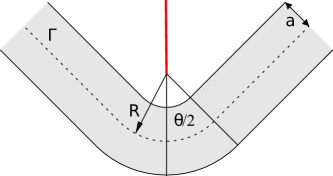
Figure 1: The geometry of the piecewise smooth curve (15) and its $a$-tubular neighbourhood

. The red line depicts the cut-locus $\mathrm{Cut}(\Gamma)$.

The case $\theta=0$ corresponds to $\Gamma$ being a straight line, while the other extreme situation $\theta=\pi$ is a union of a semi-circle and two parallel semi-lines, see Figure 2.

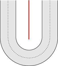
$\theta=0$		$\theta=\pi$

Figure 2: Extreme cases of the geometry setting (15).

Except for $\theta=0$, the curve $\Gamma$ is not $C^{2}$-smooth, but it is $C^{1,1}$-smooth and in fact piecewise analytic. While the cut-locus of a non-smooth submanifold in a Riemannian manifold is potentially a subtle object (cf. [9]), it is reasonable in our case. Except for $\theta=0$ when the cut-locus is empty, it is just a semi-line

$$\mathrm{Cut}(\Gamma)=\{(0,y):\ y\geq R\}\qquad\mbox{whenever}\qquad\theta\in(0,\pi]\,.$$

At the same time, $\mathrm{Cut}_{0}(\Gamma)=(0,R)$ for every $\theta\in(0,\pi]$. Consequently, we have $c_{-}(s)=+\infty$ for all $s\in\mathbb{R}$ and

$$c_{+}(s)=\begin{cases}\frac{-s+R(\tan\frac{\theta}{2}-\frac{\theta}{2})}{\tan\frac{\theta}{2}}&\mbox{if}\quad s\leq-\frac{\theta}{2}R\,,\\ R&\mbox{if}\quad-\frac{\theta}{2}R<s<\frac{\theta}{2}R\,,\\ \frac{s+R(\tan\frac{\theta}{2}-\frac{\theta}{2})}{\tan\frac{\theta}{2}}&\mbox{if}\quad s\geq\frac{\theta}{2}R\,.\end{cases}$$ (17)

Strictly speaking, the formula for $c_{+}$ makes sense only if $\theta\in(0,\pi)$, but the extreme situations can be recovered after taking the respective one-sided limits $\theta\to 0^{+}$ or $\theta\to\pi^{-}$; namely, $c_{+}(s)=+\infty$ for all $s\in\mathbb{R}$ if $\theta=0$ and $c_{+}(s)=R$ for all $s\in\mathbb{R}$ if $\theta=\pi$.

It is easy to see that (9) and (10) hold for every $a<R$ if $\theta\in(0,\pi]$ and any $a$ if $\theta=0$. The parallel coordinates described in the preceding section extend to the present non-smooth case without any changes. Moreover, because of the special structure of the cut-locus, the formula (14) becomes extremely useful for developing the usual test-function argument.

4 Existence of bound states

We assume that the $V$ is either the distribution (4) or it is an essentially bounded function satisfying (11). Then the corresponding one-dimensional operator

$$T:=-\partial_{t}^{2}+W(t)\qquad\mbox{in}\qquad L^{2}(\mathbb{R})$$

with form domain $H^{1}(\mathbb{R})$ (the sum should be understood as the form sum in the case (4)) has the essential spectrum covering $[0,\infty)$ in both cases. From now we assume that $W$ is attractive in the sense that

$$T$$ possesses at least one simple negative eigenvalue. (18)

Remark 1.

Hypothesis (18) always holds in the leaky case (4), because $\alpha$ is assumed to be a negative constant. In general, a sufficient condition to guarantee (18) is that $\int W\,<0$ (which particularly involves negative potentials of [3]). Moreover, it is easy to design potentials which simultaneously satisfy $\int W\,\geq 0$ and (18) (e.g., it is enough to consider the strong coupling regime of any $W$ possessing a negative minimum, see [6, Thm. 4]).

Let $E_{1}<0$ denote the lowest discrete eigenvalue of $T$ (explicitly, $E_{1}=-\frac{\alpha^{2}}{4}$ in the case (4)). It is well known that $E_{1}$ is simple and that the corresponding eigenfunction $\xi_{1}$ can be chosen to be positive. We additionally choose the eigenfunction to be normalised to $1$ in $L^{2}(\mathbb{R})$. Explicitly, $\xi_{1}(t)=\sqrt{\frac{|\alpha|}{4}}e^{\frac{\alpha}{2}|t|}$ in the leaky case (4). In any case, one knows that $\xi_{1}\in H^{1}(\mathbb{R})\cap L^{\infty}(\mathbb{R})$ and that the following identities hold true:

$$\xi_{1}(t)=N_{\pm}e^{\mp\sqrt{-E_{1}}t}\qquad\mbox{for every}\qquad\pm t>a\,,$$ (19)

where $N_{\pm}$ are positive constants.

At the same time, for every positive number $R$, let us consider the double-well operator

$$T_{R}:=-\partial_{t}^{2}+W(t-R)+W(-t-R)\qquad\mbox{in}\qquad L^{2}(\mathbb{R})\,.$$

Again, $\sigma_{\mathrm{ess}}(T_{R})=[0,\infty)$ and (18) ensures that $T_{R}$ possesses at least one negative eigenvalue. Let us denote by $E_{1,R}$ the lowest one and let $\xi_{1,R}$ be a corresponding eigenfunction. One has the following strict inequality.

Proposition 1.

Assume (18). Then

$$E_{1,R}<E_{1}\,.$$ (20)

Proof.

The variational definition of $E_{1,R}$ reads

$$E_{1,R}=\inf_{\stackrel{{\scriptstyle[}}{{\psi}}\not=0]{}{\psi\in H^{1}(\mathbb{R})}}\frac{Q_{R}[\psi]}{\displaystyle\int_{\mathbb{R}}|\psi(t)|^{2}\,\mathrm{d}t}\,,$$

where

$$Q_{R}[\psi]:=\int_{\mathbb{R}}|\dot{\psi}(t)|^{2}\,\mathrm{d}t+\int_{\mathbb{R}}W(t+R)\,|\psi(t)|^{2}\,\mathrm{d}t+\int_{\mathbb{R}}W(-t-R)\,|\psi(t)|^{2}\,\mathrm{d}t\,.$$

Using

$$\psi(t):=\begin{cases}\xi_{1}(t-R)&\mbox{if}\quad t\geq 0\,,\\ \xi_{1}(-t-R)&\mbox{if}\quad t<0\,,\end{cases}$$

as the test function and integrating by parts, one finds

$$Q_{R}[\psi]=E_{1}\int_{\mathbb{R}}|\psi(t)|^{2}\,\mathrm{d}t+\big{[}\bar{\psi}\dot{\psi}\big{]}_{0^{+}}^{0^{-}}\,,$$

where

$$\big{[}\bar{\psi}\dot{\psi}\big{]}_{0^{+}}^{0^{-}}=\xi_{1}(-R)\left(\dot{\xi}_{1}(-R^{-})-\dot{\xi}_{1}(-R^{+})\right)=-2\sqrt{-E_{1}}\,N_{-}^{2}e^{-2\sqrt{-E_{1}}R}\,<0\,,$$

which proves the desired claim. ∎

Note that the inequality $E_{1,R}<E_{1}$ holds in the case (4) as well. This follows directly from the argument derived in the proof of [11, Lem. 2.3].

Now we are in a position to localise the essential spectrum of $H$.

Proposition 2.

Let $\Gamma$ be given by (15). Let $V$ satisfy (11) and (18). Then

$$\sigma_{\mathrm{ess}}(H)=\begin{cases}[E_{1},\infty)&\mbox{if}\quad\theta\in[0,\pi)\,,\\ [E_{1,R},\infty)&\mbox{if}\quad\theta=\pi\,.\end{cases}$$

Proof.

The case $\theta=0$ follows trivially by a separation of variables (in fact, $\sigma(H)=[E_{1},\infty)$ if $\theta=0$). The cases $\theta\in[0,\pi)$ are due to [2, Prop. 3.1] (the lack of smoothness is not essential for the arguments given there). It remains to analyse the pathological situation $\theta=\pi$. The result is intuitively clear because the essential spectrum is determined by the behaviour at infinity only. To prove it rigorously, we proceed similarly to [11, Sec. 3].

To show that $\inf\sigma_{\mathrm{ess}}(H)\geq E_{1,R}$, we divide $\mathbb{R}^{2}$ into three subdomains

$$\Omega_{1} :=\mathbb{R}\times(R,\infty)\,,$$

$$\Omega_{2} :=(-2R,2R)\times(-R,R)\,,$$

$$\Omega_{3} :=\mathbb{R}^{2}\setminus\overline{(\Omega_{1}\cup\Omega_{2})}\,,$$

and consider an auxiliary operator $H^{N}$ which acts in the same way as $H$ but satisfies Neumann conditions on the boundaries of the subdomains. Since $H^{N}=H_{1}^{N}\oplus H_{2}^{N}\oplus H_{3}^{N}$, where $H_{\iota}^{N}$ with $\iota\in\{1,2,3\}$ is an operator in $L^{2}(\Omega_{\iota})$ which acts in the same way as $H$ but satisfies Neumann conditions on $\partial\Omega_{\iota}$, the minimax principle implies

$$\inf\sigma_{\mathrm{ess}}(H)\geq\min\sigma_{\mathrm{ess}}(H^{N})=\min\left\{\inf\sigma_{\mathrm{ess}}(H_{1}^{N}),\inf\sigma_{\mathrm{ess}}(H_{2}^{N}),\inf\sigma_{\mathrm{ess}}(H_{3}^{N})\right\}.$$

Since $H_{2}^{N}$ acts in a regular bounded domain, its spectrum is purely discrete, so it does not contribute (conventionally, $\inf\sigma_{\mathrm{ess}}(H_{2}^{N})=\infty$). Since the subdomain $\Omega_{3}$ does not intersect the support of $V$, the operator $H_{3}^{N}$ acts as the Laplacian, so $\inf\sigma_{\mathrm{ess}}(H_{3}^{N})\geq\inf\sigma(H_{3}^{N})\geq 0$. Finally, the spectral problem for $H_{1}^{N}$ can be found by a separation of variables with the result $\sigma(H_{1}^{N})=\sigma_{\mathrm{ess}}(H_{1}^{N})=[E_{1,R},\infty)$.

To show that $\sigma_{\mathrm{ess}}(H)\supset[E_{1,R},\infty)$, we construct an explicit Weyl sequence by mollifying the function $(x,y)\mapsto\xi_{1}(x)\,e^{iky}$ and localising it at infinity $y\to\infty$ We refer to [11, Sec. 3.2] for more details. ∎

Remark 2.

The part of the proposition for $\theta=\pi$ shows that condition [2, Ass. (c)] is necessary to have the stability of the essential spectrum.

Now we turn to the existence of the spectrum below the bottom of the essential spectrum.

Theorem 1.

Let $\Gamma$ be given by (15). Moreover, assume that $V$ satisfy (11) and (18). If $\theta\in(0,\pi)$, then

$$\inf\sigma(H)<E_{1}\,.$$

Proof.

Let us introduce the shifted form $\tilde{Q}[\psi]:=Q[\psi]-E_{1}\|\psi\|^{2}$. It is enough to find a test function $\psi\in\mathop{\mathrm{dom}}\nolimits Q$ such that $\tilde{Q}[\psi]<0$. Then the desired result follows by the minimax principle. The idea which comes back to [7] (see [13] for necessary mathematical adaptations) is to use a mollification of $\xi_{1}$ as the test function.

Given $n\in\mathbb{N}^{*}:=\mathbb{N}\setminus\{0\}$ (natural numbers contain zero in our convention), let $\varphi_{n}:\mathbb{R}\to\mathbb{R}$ be the real-valued function satisfying $\varphi_{n}(s)=1$ for $|s|\leq n$, $\varphi_{n}(s)=0$ for $|s|\geq 2n$ and $\varphi_{n}(s)=(2n-|s|)/n$ for $n<|s|<2n$. Then $\|\dot{\varphi}_{n}\|_{L^{2}(\mathbb{R})}^{2}=2/n\to 0$ and $\varphi_{n}\to 1$ pointwise as $n\to\infty$.

We define $\psi_{n}(s,t):=\varphi_{n}(s)\xi_{1}(t)$ and choose $n$ so large that $\varphi_{n}=1$ on the interval $I:=(-\frac{\theta}{2}R,\frac{\theta}{2}R)$ on which $\kappa$ is non-trivial. Because of the symmetry of $\Gamma$, one really has $\psi_{n}\in\mathop{\mathrm{dom}}\nolimits Q$. Let us write $\tilde{Q}=\tilde{Q}_{1}+\tilde{Q}_{2}$, where the parts $\tilde{Q}_{1}$, $\tilde{Q}_{2}$ are defined below.

For the first part $\tilde{Q}_{1}$, we have

$$\tilde{Q}_{1}[\psi_{n}]:= \int_{U}\frac{|\partial_{s}\psi_{n}|^{2}}{1-\kappa(s)t}\,\mathrm{d}s\,\mathrm{d}t$$

$$= \ \int_{\mathbb{R}}\int_{-c_{-}(s)}^{c_{+}(s)}|\dot{\varphi}_{n}(s)|^{2}|\xi_{1}(t)|^{2}\,\mathrm{d}t\,\mathrm{d}s$$

$$\leq \|\dot{\varphi}_{n}\|_{L^{2}(\mathbb{R})}^{2}\|\xi_{1}(t)\|_{L^{2}(\mathbb{R})}^{2}$$

$$= \frac{2}{n}\xrightarrow[n\to\infty]{}0\,.$$

For the second part $\tilde{Q}_{2}$, integrating by parts (twice), we have

$$\tilde{Q}_{2}[\psi_{n}]:= \int_{U}|\partial_{t}\psi_{n}|^{2}(1-\kappa(s)t)\,\mathrm{d}s\,\mathrm{d}t+\int_{U}W(t)\,|\psi_{n}|^{2}(1-\kappa(s)t)\,\mathrm{d}s\,\mathrm{d}t-E_{1}\int_{U}|\psi_{n}|^{2}(1-\kappa(s)t)\,\mathrm{d}s\,\mathrm{d}t$$

$$= \int_{U}\kappa(s)|\varphi_{n}(s)|^{2}\xi_{1}(t)\dot{\xi}_{1}(t)\,\mathrm{d}s\,\mathrm{d}t+\int_{\mathbb{R}}|\varphi_{n}(s)|^{2}\left[\xi_{1}(t)\dot{\xi}_{1}(t)(1-\kappa(s)t)\right]_{t=-c_{-}(s)}^{t=c_{+}(s)}\ \mathrm{d}s$$

$$= \int_{\mathbb{R}}|\varphi_{n}(s)|^{2}\left[\frac{1}{2}\xi_{1}(t)^{2}\kappa(s)+\xi_{1}(t)\dot{\xi}_{1}(t)(1-\kappa(s)t)\right]_{t=-c_{-}(s)}^{t=c_{+}(s)}\mathrm{d}s\,.$$

Hence, $\tilde{Q}_{2}[\psi_{n}]=\tilde{Q}_{2}^{\mathrm{int}}[\psi_{n}]+\tilde{Q}_{2}^{\mathrm{ext}}[\psi_{n}]$, where the forms on the right-hand side correspond to dividing the last integral to an integration over $I$ and $\mathbb{R}\setminus I$, respectively. Explicitly,

$$\tilde{Q}_{2}^{\mathrm{int}}[\psi_{n}] =\int_{I}\left[\frac{1}{2}\xi_{1}(t)^{2}\kappa(s)+\xi_{1}(t)\dot{\xi}_{1}(t)(1-\kappa(s)t)\right]_{t=-c_{-}(s)}^{t=c_{+}(s)}\ \mathrm{d}s\,,$$

$$\tilde{Q}_{2}^{\mathrm{ext}}[\psi_{n}] =\int_{\mathbb{R}\setminus I}|\varphi_{n}(s)|^{2}\left[\xi_{1}(t)\dot{\xi}_{1}(t)\right]_{t=-c_{-}(s)}^{t=c_{+}(s)}\mathrm{d}s=-\sqrt{-E_{1}}\int_{\mathbb{R}\setminus I}|\varphi_{n}(s)|^{2}\left[\xi_{1}(c_{+}(s))^{2}+\xi_{1}(-c_{-}(s))^{2}\right]\mathrm{d}s\,,$$

where the last equality is due to (19). Here $\tilde{Q}_{2}^{\mathrm{int}}[\psi_{n}]$ is of course finite and in fact independent of $n$ (because $\varphi_{n}=1$ on $I$). Since $\tilde{Q}_{2}^{\mathrm{ext}}[\psi_{n}]$ is negative for every $n$, the limit

$$\lim_{n\to\infty}\tilde{Q}_{2}^{\mathrm{ext}}[\psi_{n}]=-\sqrt{-E_{1}}\int_{\mathbb{R}\setminus I}\left[\xi_{1}(c_{+}(s))^{2}+\xi_{1}(-c_{-}(s))^{2}\right]\mathrm{d}s$$

is well defined (it can be $-\infty$, namely if $\theta=-\pi$, see Remark 3 below).

In summary,

$$\lim_{n\to\infty}\tilde{Q}[\psi_{n}]=\tilde{Q}_{2}^{\mathrm{int}}[\psi_{n}]+\lim_{n\to\infty}\tilde{Q}_{2}^{\mathrm{ext}}[\psi_{n}]\\ =\int_{I}\left[\frac{1}{2}\xi_{1}(t)^{2}\kappa(s)+\xi_{1}(t)\dot{\xi}_{1}(t)(1-\kappa(s)t)\right]_{t=-c_{-}(s)}^{t=c_{+}(s)}\ \mathrm{d}s-\sqrt{-E_{1}}\int_{\mathbb{R}\setminus I}\left[\xi_{1}(c_{+}(s))^{2}+\xi_{1}(-c_{-}(s))^{2}\right]\mathrm{d}s\,.$$

Using the special form of $\Gamma$ in this general result, namely the formulae (16) and (17), one finds

$$\tilde{Q}_{2}^{\mathrm{int}}[\psi_{n}]=\xi_{1}(R)^{2}\mbox{$\frac{\theta}{2}$}\,,\qquad\lim_{n\to\infty}\tilde{Q}_{2}^{\mathrm{ext}}[\psi_{n}]=-\xi_{1}(R)^{2}\tan\mbox{$\frac{\theta}{2}$}\,.$$

We finally arrive at

$$\lim_{n\to\infty}\tilde{Q}[\psi_{n}]=\xi_{1}(R)^{2}\,(\mbox{$\frac{\theta}{2}$}-\tan\mbox{$\frac{\theta}{2}$})<0\,.$$ (21)

In these circumstances, we can therefore find a positive $n_{0}$ such that $\tilde{Q}[\psi_{n}]<0$ for every $n\geq n_{0}$. ∎

Remark 3.

The theorem is valid also for $\theta=\pi$. Indeed, then the right-hand side equals $-\infty$, because $\tilde{Q}_{2}^{\mathrm{ext}}[\psi_{n}]$ tends to $-\infty$ as $n\to\infty$ while $\tilde{Q}_{2}^{\mathrm{int}}[\psi_{n}]$ is independent of $n$. Hence the conclusion of the proof holds as well. However, in this case, the result also follows from Propositions 1 and 2.

As a direct combination of Theorem 1 with Proposition 2, we get the following ultimate result about the existence of discrete spectra in soft and leaky waveguides.

Corollary 1.

Let $\Gamma$ be given by (15). Moreover, assume that $V$ satisfy (11) and (18). If $\theta\in(0,\pi)$, then

$$\sigma_{\mathrm{disc}}(H)\not=\varnothing\,.$$

Remark 4.

Note that the discrete spectrum is obviously empty for the straight waveguide corresponding to $\theta=0$. In this paper we leave the problem of the existence of discrete eigenvalues for $\theta=\pi$ open. Also it arises a natural question about spectral properties of the system if $\theta\to\pi^{-}$. One may expect that in this case the number of discrete eigenvalues goes to infinity. Therefore the question is: what is the asymptotics of the counting function for $\theta\to\pi^{-}$?

Acknowledgment

D.K. was supported by the EXPRO grant No. 20-17749X of the Czech Science Foundation. J. K. was supported by Internal Project of Excellent Research of the Faculty of Science of University Hradec Králové, “Studying of properties of confined quantum particle using Woods-Saxon potential”.

References

[1]
I. Chavel, Riemannian Geometry: A Modern Introduction, Cambridge University Press,
1993.
[2]
P. Exner, Leaky quantum graphs: a review, Analysis on Graphs and its
Applications, Cambridge, 2007 (P. Exner et al., ed.), Proc. Sympos. Pure
Math., vol. 77, Amer. Math. Soc., Providence, RI, 2008, pp. 523–564.
[3]
, Spectral properties of soft quantum waveguides, J. Phys. A:
Math. Gen. (2020), to appear.
[4]
P. Exner and T. Ichinose, Geometrically induced spectrum in curved leaky
wires, J. Phys A 34 (2001), 1439–1450.
[5]
P. Exner and P. Šeba, Bound states in curved quantum waveguides,
J. Math. Phys. 30 (1989), 2574–2580.
[6]
P. Freitas and D. Krejčiřík, Damped wave equation in
unbounded domains, J. Differential Equations 211 (2005), no. 1,
168–186.
[7]
J. Goldstone and R. L. Jaffe, Bound states in twisting tubes, Phys.
Rev. B 45 (1992), 14100–14107.
[8]
S. Haag, J. Lampart and S. Teufel,
Generalised Quantum Waveguides,
Ann. Hen. Poinc. 16 (2015), 2535–2568.
[9]
J.-I. Itoh, The length of a cut locus on a surface and Ambrose’s
problem, J. Differential Geom. 43 (1996), 642–651.
[10]
T. Kato, Perturbation theory for linear operators, Springer-Verlag,
Berlin, 1966.
[11]
S. Kondej and D. Krejčiřík, Spectral analysis of a quantum
system with a double line singular interaction, Publ. RIMS, Kyoto University
49 (2013), 831–859.
[12]
, Asymptotic spectral analysis in colliding leaky quantum layers,
J. Math. Anal. Appl. 446 (2017), 1328–1355.
[13]
D Krejčiřík and J. Kříž, On the spectrum of
curved quantum waveguides, Publ. RIMS, Kyoto University 41 (2005),
no. 3, 757–791.
[14]
J. Wachsmuth and S. Teufel, Effective Hamiltonians for constrained quantum systems, Mem. Am. Math. Soc. 230 (2014), no. 1083 (93 pages).