Ultra-short-period Planets are Stable Against Tidal Inspiral

Abstract

It has been unambiguously shown in both individual systems and at the population level that hot Jupiters experience tidal inspiral before the end of their host stars’ main sequence lifetimes. Ultra-short-period (USP) planets have orbital periods $P<1$ day, rocky compositions, and are expected to experience tidal decay on similar timescales to hot Jupiters if the efficiency of tidal dissipation inside their host stars parameterized as $Q_{\ast}^{\prime}$ is independent of $P$ and/or secondary mass $M_{\mathrm{p}}$. Any difference between the two classes of systems would reveal that a constant $Q_{\ast}^{\prime}$ model is insufficient. If USP planets experience tidal inspiral, then USP planet systems will be relatively young compared to similar stars without USP planets. Because it is a proxy for relative age, we calculate the Galactic velocity dispersions of USP planet candidate host and non-host stars using data from Gaia Data Release 2 supplemented with ground-based radial velocities. We find that main sequence USP planet candidate host stars have kinematics consistent with similar stars in the Kepler field without observed USP planets. This indicates that USP planet hosts have similar ages as field stars and that USP planets do not experience tidal inspiral during the main sequence lifetimes of their host stars. The survival of USP planets requires that $Q_{\ast}^{\prime}\gtrsim 10^{7}$ at $P\approx 0.7$ day and $M_{\mathrm{p}}\approx 2.6~{}M_{\earth}$. This result demands that $Q_{\ast}^{\prime}$ depend on the orbital period and/or mass of the secondary in the range $0.5\mathrm{~{}days}\lesssim P\lesssim 5$ days and $1~{}M_{\oplus}\lesssim M_{\mathrm{p}}\lesssim 1000~{}M_{\oplus}$.

1 Introduction

Hamer & Schlaufman (2019) demonstrated unambiguously at the population level that hot Jupiters are destroyed by tides during the main sequence lifetimes of their host stars. Soon after, Yee et al. (2020) showed that the departure from a linear ephemeris in the WASP-12 system could only be explained by tidal decay. These discoveries ended 25 years of uncertainty regarding the stability of close-in giant planets against orbital decay due to tidal interactions with their host stars.

With orbital periods $P<1$ day, ultra-short-period (USP) planets are an even more extreme population than hot Jupiters. CoRoT-7 b, the first transiting terrestrial exoplanet to be detected, is a USP planet with $P=0.85$ days (Léger et al., 2009). It was subsequently shown that CoRoT-7 is a multiple-planet system (Queloz et al., 2009). Following this discovery, Schlaufman et al. (2010) explained the existence of CoRoT-7-like systems as a consequence of convergent Type I migration in multiple-planet systems which is terminated at their parent protoplanetary disks’ magnetospheric truncation radii. Following disk dissipation, secular interactions between planets maintain non-zero eccentricities in a system’s innermost planet, thereby causing the orbital decay of that planet due to tidal dissipation within it as circularization occurs. This process continues until the innermost planet secularly decouples from the rest of the planets in a system, halting its inward drift at $P<1$ day. They argued that a population of multiple-planet systems like these would be discovered by Kepler.

Kepler would go on to discover more than one hundred USP planets and planet candidates, many in multiple planet systems (e.g., Batalha et al., 2011; Fressin et al., 2011; Sanchis-Ojeda et al., 2013). A uniform analysis of the first 16 quarters of Kepler data by Sanchis-Ojeda et al. (2014) revealed that USP planet candidates have planet radii $R_{\mathrm{p}}<2~{}R_{\earth}$ and occur around less than 1% of GK dwarfs. The sub-day orbital periods of USP planets mean that they should experience significant tidal interactions with their host stars. As we will show in Section 3, if the efficiency of tidal dissipation within the host stars of USP planets is the same as in hosts of hot Jupiters, then USP planets should inspiral on a similar timescale.

There is reason to believe that the lower masses and shorter periods of USP planets relative to hot Jupiters might affect the efficiency of tidal dissipation within their host stars. Detailed theoretical models of nonlinear dissipation by internal gravity waves in stellar hosts indicate that massive, short-period planets can trigger especially efficient dissipation (e.g., Barker & Ogilvie, 2010; Essick & Weinberg, 2016). It may be that hot Jupiters can trigger this mode of dissipation, while the lower-mass USP planets cannot. On the other hand, observations of hot Jupiter systems have provided empirical evidence that shorter period systems experience less efficient dissipation (Penev et al., 2018). The extremely short orbital periods of USP planets may therefore spare them from destruction.

The efficiency of tidal dissipation in USP planet host stars also plays an important role in some models of their formation. Lee & Chiang (2017) proposed a model that reproduced planet occurrence as a function of period in which proto-USP planets form uniformly distributed in $\log_{10}(P)$. USP planets are then brought to their observed locations by orbital decay due to tidal dissipation within their host stars. Other models do not rely on tidal dissipation within host stars to explain the formation of USP planets and instead appeal to tidal dissipation within the planet (e.g., Schlaufman et al., 2010; Petrovich et al., 2019).

The efficiency of tidal dissipation inside USP planet host stars has important consequences for both USP formation and evolution specifically, as well as our understanding of tidal dissipation in general. As shown in Hamer & Schlaufman (2019), systems hosting exoplanets destined to be destroyed by tides will appear younger than a similar population of stars without such planets. In short, if USP planets are destroyed due to tides, then USP planet host stars will be younger than similar stars without USP planets.

To evaluate their relative ages, in this paper we compare the Galactic velocity dispersions of Sanchis-Ojeda et al. (2014) USP planet candidate host stars and stars without USP planets. We show that these two populations have indistinguishable kinematics and therefore similar ages. This observation implies that USP planets do not experience tidal inspiral during the main sequence lifetimes of their host stars. The efficiency of tidal dissipation inside a planet host star must therefore depend on the amplitude and/or frequency of tidal forcing. This paper is organized as follows. In Section 2, we describe our USP planet candidate host and field star samples. In Section 3, we outline our methods to make a robust comparison between the Galactic velocity dispersions of the two samples. In Section 4, we discuss the implications of our result for theories of tidal dissipation and USP planet formation. We conclude in Section 5.

2 Data

We obtain our sample of USP planet candidate hosts from Sanchis-Ojeda et al. (2014). Those authors used Fourier-transformed Kepler Q1–Q16 light curves to identify candidate transiting planets with $P<1$ day. These systems were combined with additional candidate planets with $P<1$ day from the KOI list as of January 2014 (Mullally et al., 2015), as well as 28 candidates from other independent searches (Ofir & Dreizler, 2013; Huang et al., 2013; Jackson et al., 2013). These candidates were then vetted by a homogeneous series of tests designed to identify false-positive signals. This search resulted in a sample of 106 well-vetted USP planet candidates.

We obtain the Gaia Data Release 2 (DR2) designations of these USP planet candidate host stars from SIMBAD and then query the Gaia Archive to retrieve the astrometric and radial velocity data required to calculate the kinematics of the sample. Most of the stars have Gaia $G$-band magnitude $G\gtrsim 16$, making them too faint to have radial velocities available in Gaia DR2. We obtain radial velocities for these faint stars by supplementing our sample with radial velocities (in order of priority) from the California-Kepler Survey (CKS - Petigura et al., 2017), the Apache Point Observatory Galactic Evolution Experiment (APOGEE - Majewski et al., 2017) DR16, and the Large Sky Area Multi-Object Fiber Spectroscopic Telescope (LAMOST) DR5 (Luo et al., 2019). The majority of the radial velocities for the USP planet candidate host stars come from the CKS. We apply the data quality cuts described in Hamer & Schlaufman (2019) and reproduced in the Appendix to ensure reliable kinematics.

We provide in Table 1 the 68 USP planet candidate hosts in our sample, their KIC identifiers, Gaia DR2 designations, radial velocities, periods, radii, and masses. Using the Brewer & Fischer (2018) isochrone-derived values for host stellar radii $R_{\ast}$ and transit depths from Sanchis-Ojeda et al. (2014) we calculate $R_{\mathrm{p}}$. We then calculate planet mass $M_{\mathrm{p}}$ for the USP planet candidates in our sample by fitting a spline to the Earth-like composition mass–radius curve from Zeng et al. (2019).

Table 1: Ultra-short-period Planet Hosts

KIC ID	Gaia DR2 source_id	Radial Velocity		Period	Planet Radius	Estimated Mass
		(km s-1)		(days)	($R_{\oplus}$)	($M_{\oplus}$)
6750902	2116704610985856512	-17.00	0.469	2.579_-0.105^+0.083	50.936_-10.699^+10.927
10186945	2119583510383666560	-12.60	0.397	1.095_-0.029^+0.017	1.394_-0.133^+0.081
10319385	2119593990103923840	-38.40	0.689	1.611_-0.031^+0.017	5.856_-0.428^+0.244
9873254	2119511080054847616	-8.10	0.900	0.801_-0.036^+0.035	0.444_-0.068^+0.074
6666233	2104748521545492864	-51.43	0.512	⋯	⋯
10647452	2107681262654003328	-15.60	0.763	1.271_-0.080^+0.056	2.409_-0.514^+0.411
5340878	2103579397088495616	-10.90	0.540	⋯	⋯
6755944	2104890633423618048	4.60	0.693	1.065_-0.033^+0.029	1.256_-0.136^+0.129
5513012	2103628462794226304	-11.60	0.679	1.523_-0.037^+0.029	4.699_-0.418^+0.355
6265792	2103743018162573952	6.80	0.935	1.169_-0.047^+0.043	1.776_-0.251^+0.254

Note. — Table 1 is ordered by right ascension and is published in its entirety in machine-readable format. Planets without radius and mass estimates did not have their host stars’ radii presented in Brewer & Fischer (2018).

To evaluate the relative age of the USP planet candidate host population, we need a sample of similar field stars with no detected USP planets. As all of our USP planet candidate hosts lie in the Kepler field, we select as our comparison sample all stars that were observed for at least one quarter as part of Kepler’s planet search program. By selecting both samples from the Kepler field, we are ensuring that the sample of stars not hosting planets has been thoroughly searched for USP planets. Sanchis-Ojeda et al. (2014) found that the occurrence of USP planets is less than 1% for GK dwarfs, so any contamination by undetected USP planets should be minimal. Additionally, as both samples of stars are colocated in the Kepler field any kinematic differences cannot be attributed to Galactic structure. For these non-host stars, we use SIMBAD to obtain their Gaia DR2 identifiers, and query the Gaia Archive for their DR2 data. As with the sample of USP planet candidate host stars, many of the stars are too faint to have had their radial velocities measured by Gaia. We obtain radial velocities for these stars with ground-based radial velocities from (in order of priority) the CKS, APOGEE DR16, and LAMOST DR5. Most of the radial velocities for the field star sample come from LAMOST DR5.

To determine if USP planets tidally inspiral during the main sequence lifetimes of their host stars, we must limit our sample of planet candidate hosts and non-hosts to main sequence stars. To do so, we exclude all stars more than one magnitude above the Pleiades solar metallicity zero-age main sequence from Hamer & Schlaufman (2019). Before applying this cut, we correct for extinction and reddening of the stars in both samples using a three-dimensional extinction map (Capitanio et al., 2017). For a star in our sample, we interpolate the grid of extinction values out to the star, and integrate along the line-of-sight to calculate a total $E(B-V)$ reddening. We convert $E(B-V)$ to $E(G_{\mathrm{BP}}-G_{\mathrm{RP}})$ using the mean extinction coefficients from Casagrande & VandenBerg (2018). We illustrate this calculation in Figure 1.

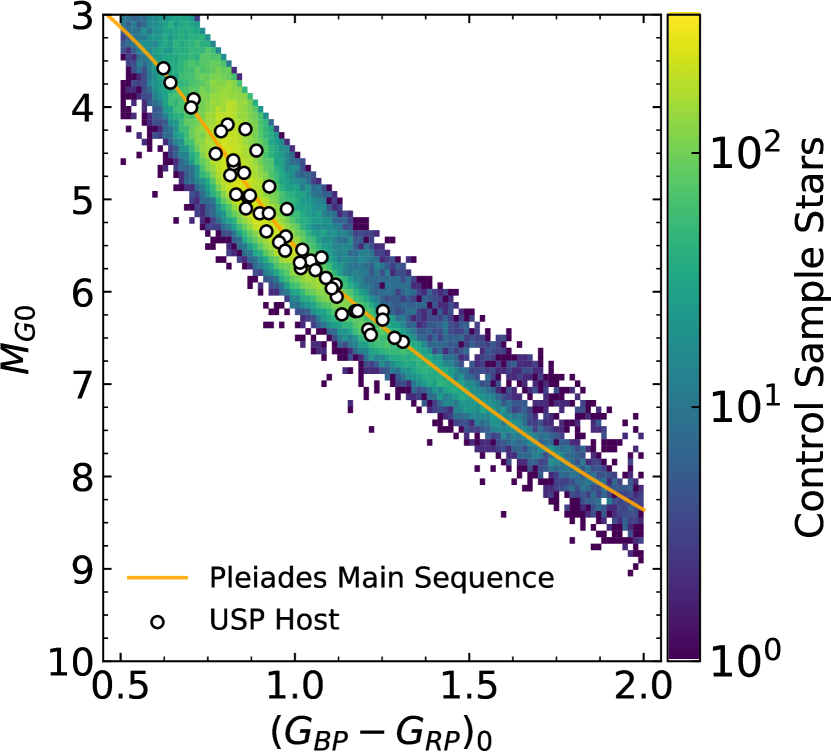
Figure 1: USP planet candidate host and field star samples. We plot USP planet candidate hosts as white points with black outlines and the density of stars in the field star sample as the background color map. We indicate the Pleiades main sequence spline fit from Hamer & Schlaufman (2019) used to remove evolved stars as the orange line.

3 Analysis

If one assumes that tidal dissipation within the host stars of USP planets occurs with the same efficiency as in hot Jupiter hosts, then it can be shown that USP planets should inspiral more quickly than hot Jupiters. Assuming that all dissipation occurs in the host star—a safe assumption for tidally locked planets—the inspiral time can written

$$t_{\mathrm{in}}=\frac{2}{13}\frac{2Q_{\ast}^{\prime}}{9}\frac{M_{\ast}}{M_{\mathrm{p}}}\left(\frac{a}{R_{\ast}}\right)^{5}\frac{P}{2\pi},$$ (1)

as in Hamer & Schlaufman (2019). Here $Q_{\ast}^{\prime}$ is the modified stellar tidal quality factor, a parameter describing the efficiency of tidal dissipation, $M_{\ast}$ is stellar mass, $a$ is the orbital semi-major axis, and $R_{\ast}$ is the stellar radius. It follows that the ratio of the inspiral time of a USP planet to that of a hot Jupiter around an identical star with identical $Q_{\ast}^{\prime}$ is

$$\frac{t_{\mathrm{in,USP}}}{t_{\mathrm{in,HJ}}}=\frac{M_{\mathrm{HJ}}}{M_{\mathrm{USP}}}\left(\frac{P_{\mathrm{USP}}}{P_{\mathrm{HJ}}}\right)^{13/3},$$ (2)

by Kepler’s third law. The median period of hot Jupiters in the Hamer & Schlaufman (2019) sample was 3.4 days, whereas the median period of USP planet candidates analyzed in this paper is 0.7 days. Similarly, the median mass of hot Jupiters in the Hamer & Schlaufman (2019) sample was $290~{}M_{\oplus}$ while the median mass of USP planets analyzed in this paper is $2.6~{}M_{\oplus}$. As a result $t_{\mathrm{in,USP}}/t_{\mathrm{in,HJ}}\approx 0.10$. Since Hamer & Schlaufman (2019) showed that hot Jupiters inspiral during their host stars’ main sequence lifetimes, if $Q_{\ast}^{\prime}$ is the same for hot Jupiter and USP planet hosts then USP planets should inspiral as well.

If this is so, then we should see a colder Galactic velocity dispersion for USP planet host stars when compared to similar field stars. To calculate Galactic space velocities, we convert from the proper motions, radial velocities, and parallaxes described in Section 2 using pyia (Price-Whelan, 2018). A requirement of this approach is that the uncertainties on individual Galactic space velocities are small relative to the velocity dispersion of the USP planet candidate host star and field star samples. We therefore estimate Galactic space velocity uncertainties for each star using a Monte Carlo simulation. We construct the astrometric covariance matrix and sample 100 realizations from the astrometric uncertainty distributions for each star’s position, proper motions, parallax, and radial velocity using pyia. The uncertainties on position, proper motion, and parallax all come from Gaia DR2. We source radial velocities and uncertainties from the CKS, APOGEE DR16, Gaia DR2, and LAMOST DR5 in that order. The typical radial velocity precisions are 0.1, 0.5, 1.0, and 5.0 km s^-1 respectively. We construct a point estimate for each star’s velocity uncertainty by taking the standard deviation of the 100 realizations of its Galactic space velocity.

We plot in Figure 2 the individual $UVW$ velocity uncertainty distributions for both our USP planet candidate host star sample and a matched control sample (the details of this matching is described in the following paragraph). Because our inference depends on a comparison with the result from Hamer & Schlaufman (2019), we execute a similar calculation for the Hamer & Schlaufman (2019) sample. We plot the results of this calculation in Figure 2. The typical space velocities uncertainties are $\approx\!\!1$ km s^-1, much smaller than the velocity dispersion of the stellar population (see Figure 3 below). The uncertainty on $V$ for the field star sample matched to the USP hosts is larger than the uncertainties on $U$ and $W$. The reason is that the Kepler field is aligned with $V$ and the uncertainty is therefore dominated by the LAMOST radial velocity uncertainties. The typical velocity uncertainty for the USP planet candidate host stars is smaller than that of the hot Jupiter host star sample.

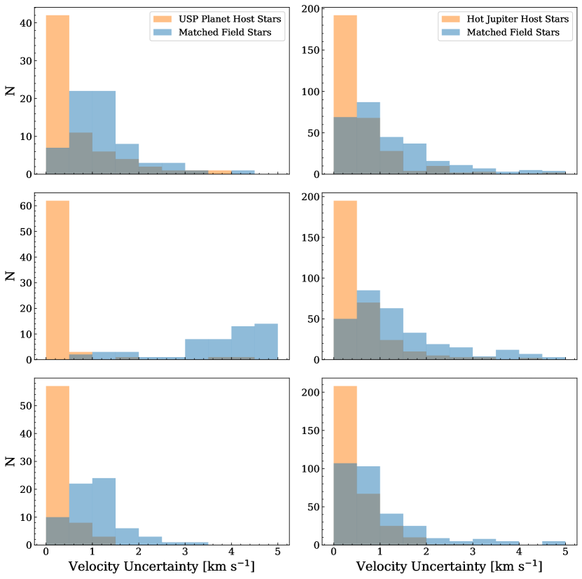
Figure 2: Distribution of $U$, $V$, and $W$ uncertainties in the top, middle, and bottom panels respectively. Left: USP planet candidate host stars in orange and a matched control sample of field stars in blue. Right: Hamer & Schlaufman (2019) hot Jupiter hosts in orange and a matched control sample of field stars in blue. The typical velocity uncertainties are less than 1 km s^-1 for USP planet candidate host stars and less than 5 km s^-1 for the matched field star sample. Both are well below the population velocity dispersions. We note that the typical velocity uncertainty in our sample of USP planet candidate host stars is smaller than the typical velocity uncertainty of the hot Jupiter host sample described in Hamer & Schlaufman (2019).

To perform a robust comparison of the kinematics of our USP planet candidate host stars and field stars, we construct samples of field stars matched to the USP planet candidate host stars on a one-to-one basis. Since Winn et al. (2017) showed that USP planet candidate host stars have a metallicity distribution indistinguishable from the field, we do not attempt to match our samples on metallicity. To mitigate possible differences in stellar mass distributions, we assemble samples of field stars matched to the sample of USP planet candidate hosts in color. Specifically, we iteratively construct a color-matched control sample by selecting 68 stars from the field star sample such that every USP planet candidate host is mirrored by a star in the control sample within 0.025 mag in $(G_{BP}-G_{RP})_{0}$. For each of these Monte Carlo iterations, we calculate the mean $UVW$ velocity and then calculate the $UVW$ velocity dispersion

$$\frac{1}{N}\sum\left[(U_{i}-\overline{U})^{2}+(V_{i}-\overline{V})^{2}+(W_{i}-\overline{W})^{2}\right]^{1/2}.$$ (3)

We plot the result of this Monte Carlo simulation in Figure 3. The USP planet candidate hosts have kinematics indistinguishable from matched samples of non-host field stars. As the Galactic velocity dispersion of a thin disk stellar population is correlated with its average age (e.g. Binney et al., 2000), the best explanation for this observation is that USP planet candidate host stars have ages consistent with the field.

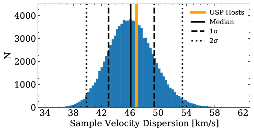
Figure 3: Velocity dispersion distribution of the matched control samples (blue histograms) compared to the velocity dispersion of our USP planet candidate host star sample (orange vertical line). The black vertical lines show the (2nd, 16th, 50th, 84th, and 98th) percentiles of the Monte Carlo samples. The USP planet candidate hosts have kinematics indistinguishable from the matched Monte Carlo samples of field stars. The only explanation for this observation is that USP planet candidate host stars are of similar age to similar non-host stars. We argue that USP planets are stable against tidal inspiral during the main sequence lifetime of their host stars.

While we argue that our observation is evidence that USP planets do not tidally inspiral, there are at least three other possible explanations which must be ruled out. Our observation could be attributed to a large number of false positives in our USP planet candidate sample. We believe this is unlikely. Sanchis-Ojeda et al. (2014) required each transit be detected with SNR $>12$ and thoroughly vetted their USP planet candidates with standard tests for false positives using Kepler data (Batalha et al., 2010). These included centroid shift checks to ensure that the photocenter did not vary with the period of the candidate, which would be indicative of a blended background eclipsing binary. They also searched for odd/even transit depth differences or phase-curve variations indicative of eclipsing binaries. As it has been shown that the false positive rate in Kepler systems with multiple transiting planets is low or even zero (e.g., Lissauer et al., 2012, 2014), the strongest evidence that many of the USP planet candidates in our sample are real is that 10 are found in multiple-planet systems. Consequently, we argue that it is highly unlikely that our sample has a high false positive rate.

Another possibility is that our sample size is too small to execute our statistical comparison. To verify that our sample size is sufficient, we perform the following test. As shown in Figure 3, the Galactic velocity dispersion of the USP planet candidate host sample is higher than 60% of the matched Monte Carlo samples of field stars. If the apparent velocity dispersion similarity is due to small number statistics inflating the USP planet candidate host velocity dispersion, then similarly-sized samples of hot Jupiter host stars would be affected in the same way. We select 1,000 random subsamples of 68 hot Jupiter hosts from the Hamer & Schlaufman (2019) sample, construct 1,000 Monte Carlo samples of field stars matched to each subsample of hot Jupiter hosts as described in Hamer & Schlaufman (2019), and determine how often the Galactic velocity dispersion of the hot Jupiter host subsample is higher than 60% of the matched Monte Carlo field star samples. The result is that identically zero of the 1,000 subsamples have a Galactic velocity dispersion as relatively high as that of the USP planet candidate hosts. As a result, we argue that there is less than a 1 in 1,000 chance that the relatively small size of the USP planet candidate host star sample affects our calculation.

It may also be that the difference in inspiral timescale between USP planet candidate and hot Jupiter systems is due to differences in the masses or radii of their host stars. Using homogeneously derived stellar parameters from Brewer et al. (2016) and Brewer & Fischer (2018), we find that the ratios of the median masses and radii of the USP planet candidate and hot Jupiter host stars are 0.85 and 0.78. Assuming similar host star masses and radii implied that $t_{\mathrm{in,USP}}/t_{\mathrm{in,HJ}}\approx 0.1$. After accounting for the difference in the median masses and radii, $t_{\mathrm{in,USP}}/t_{\mathrm{in,HJ}}$ increases to 0.29. While the median USP planet candidate and hot Jupiter host stars differ, USP planets should still inspiral on a shorter timescale than hot Jupiters if $Q_{\ast}^{\prime}$ is independent of forcing frequency and/or amplitude.

4 Discussion

We have shown that main sequence stars hosting USP planet candidates have a Galactic velocity dispersion indistinguishable from that of matched samples of stars which do not host observed USP planets. This implies that the populations have similar ages and that USP planets do not tidally inspiral during the main sequence lifetimes of their host stars. This is in sharp contrast to hot Jupiters, which have been shown to tidally inspiral on this timescale (Hamer & Schlaufman, 2019; Yee et al., 2020). As we argued above, there are no other plausible explanations for the similar kinematics of USP planet candidate hosts and non-hosts other than the robustness of USP planets to tidal inspiral. This requires that USP planets trigger less efficient dissipation within their host stars than hot Jupiters.

One possible explanation for this change in efficiency may be that $Q_{\ast}^{\prime}$ is a function of tidal forcing frequency. In this case, the shorter orbital periods of USP planets in comparison to hot Jupiters could be the key to their survival. There are both theoretical reasons (e.g. Ogilvie & Lesur, 2012; Duguid et al., 2020) to believe that this might be so and some observational evidence that $Q_{\ast}^{\prime}$ increases as orbital period decreases. Penev et al. (2018) compared the rotation rates of stars with $T_{\mathrm{eff}}<6100$ K hosting hot Jupiters with $P<3.5$ days to the expected rotation rates for similar stars without hot Jupiters. They then determined the efficiency of tidal dissipation within the host stars necessary to explain the observed rotational enhancements over the systems’ lifetimes. They found that $Q_{\ast}^{\prime}$ increases from $10^{5}$ to $10^{7}$ as the tidal period

$$P_{\mathrm{tide}}=\frac{1}{2(P_{\mathrm{orb}}^{-1}-P_{\mathrm{spin}}^{-1})},$$ (4)

decreases from 2 days to 0.5 days. This result is consistent with our inference that the tidal dissipation triggered by hot Jupiters within their host stars is more efficient than that triggered by the shorter-period USP planets.

USP planets are also two orders of magnitude less massive that hot Jupiters. Theoretical work on non-linear internal gravity waves has shown that the efficiency of tidal dissipation within stars may depend on the amplitude of tidal forcing (Barker & Ogilvie, 2010; Essick & Weinberg, 2016). According to Barker & Ogilvie (2010), the non-linear wave breaking criterion is

$$\left(\frac{M_{\mathrm{p}}}{M_{\mathrm{Jup}}}\right)\left(\frac{P}{1\mathrm{\ day}}\right)^{1/6}\gtrsim 3.3.$$ (5)

As described above, the median orbital period of hot Jupiters in the Hamer & Schlaufman (2019) sample was 3.4 days, whereas the median orbital period of USP planet candidates analyzed in this paper is 0.7 days. Because Equation (5) depends on orbital period, non-linear wave breaking might be important for planets with $M_{\mathrm{p}}\gtrsim 2.7~{}M_{\mathrm{Jup}}$ and $M_{\mathrm{p}}\gtrsim 3.5~{}M_{\mathrm{Jup}}$ at $P=3.4$ days and $P=0.7$ days. Only 44 out of 313 hot Jupiters and zero USP planet candidates satisfy Equation (5). Therefore, the Barker & Ogilvie (2010) model cannot explain the apparent difference in the efficiency of tidal dissipation we infer between hot Jupiter and USP planet systems.

Essick & Weinberg (2016) proposed that weakly non-linear gravity waves could result in amplitude-dependent $Q_{\ast}^{\prime}$ values. Those authors presented a numerical fit to their predicted tidal inspiral times which is valid for $0.5~{}M_{\mathrm{Jup}}\leq M_{\mathrm{p}}\leq 3.0~{}M_{\mathrm{Jup}}$ and $P<4$ days. None of the USP planet candidates in our sample are massive enough to trigger this mode of dissipation. Of the 50 hot Jupiters in the Hamer & Schlaufman (2019) sample for which the numerical fit is valid and for which we have homogeneously derived stellar parameters from Brewer et al. (2016) and Brewer & Fischer (2018), 16 have tidal inspiral times shorter than the main sequence lifetimes of their host stars. While weakly non-linear internal gravity waves may be capable of explaining the inspiral of a minority of hot Jupiter systems, they cannot explain the observation that most hot Jupiters do not survive their host stars’ main sequence lifetimes. The net result is that we can rule out weakly non-linear internal gravity waves as a likely explanation for the difference we infer in tidal dissipation efficiency between the hot Jupiter and USP planet regimes.

As in Hamer & Schlaufman (2019), we can derive a limit on the stellar tidal quality factor $Q_{\ast}^{\prime}$ based on our observation that USP planets do not tidally inspiral during the main sequence lifetimes of their host stars. Using homogeneously-derived stellar parameters from Brewer & Fischer (2018), we calculate the main sequence lifetime of each USP planet candidate host star according to the scaling relation

$$\frac{t_{\mathrm{MS,}\ast}}{t_{\mathrm{MS,}\odot}}=\left(\frac{M_{\ast}}{M_{\odot}}\right)^{-2.5}.$$ (6)

Finally, we solve Equation (1) for $Q_{\ast}^{\prime}$, assuming $t_{\mathrm{in}}>t_{\mathrm{MS}}$ to obtain a lower limit on $Q_{\ast}^{\prime}$ for each system

$$Q_{\ast}^{\prime}>t_{\mathrm{MS}}\frac{117}{4}\frac{M_{\mathrm{p}}}{M_{\ast}}\left(\frac{R_{\ast}}{a}\right)^{5}\frac{2\pi}{P}.$$ (7)

We plot the results of this calculation in Figure 4. Because we use a population-level approach, we can only provide constraints based on the “typical” system within our sample. We estimate $Q_{\ast}^{\prime}$ in the typical USP planet system by calculating the median $Q_{\ast}^{\prime}$ among the systems with periods that fall within the 16th and 84th period percentiles (instead considering the typical USP planet in terms of mass rather than period makes a negligible difference). We find that the survival of USP planets beyond the end of their hosts’ main sequence lifetimes requires $\log_{10}{Q_{\ast}^{\prime}}>6.96^{+0.67}_{-1.07}$.

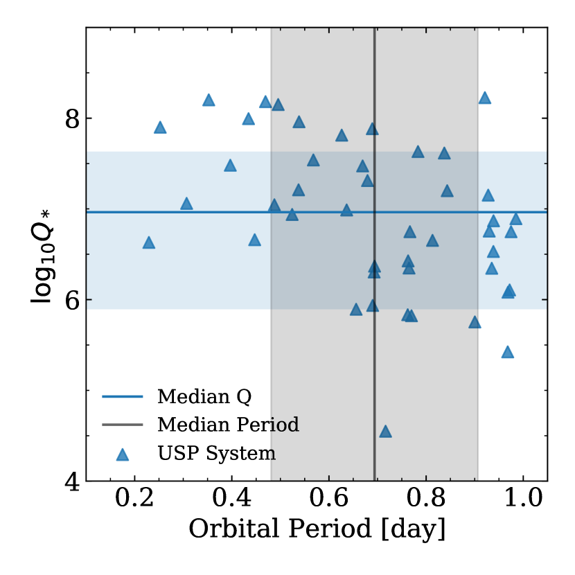
Figure 4: Minimum $Q_{\ast}^{\prime}$ required for survival of USP planets during the main sequence. We use the formalism presented in Lai (2012) and homogeneously derived spectroscopic stellar parameters from Brewer & Fischer (2018) to derive the limit on $Q_{\ast}^{\prime}$. The vertical line shows the median period of the USP planet candidate sample, whereas the gray rectangle spans the 16th to 84th percentiles of the sample period distribution (approximately 0.39 days $\lesssim P\lesssim$ 0.92 days). We calculate the minimum $Q_{\ast}^{\prime}$ required for each system, and within this period range where our velocity dispersion analysis applies, we calculate the (16,50,84) percentiles. For those systems in the gray rectangle, the horizontal line is the median $Q_{\ast}^{\prime}$ and the blue rectangle spans the 16th to 84th percentiles of the inferred $Q_{\ast}^{\prime}$ distribution. We find $\log_{10}{Q_{\ast}^{\prime}}>6.96^{+0.67}_{-1.07}$

Our observation that USP planets are robust to tidal dissipation inside their host stars also informs theories of USP planet formation. In the USP planet formation scenarios put forward by Schlaufman et al. (2010) and Petrovich et al. (2019), non-zero eccentricities of proto-USP planets are maintained due to secular interactions with more distant planets in multiple-planet systems. The Schlaufman et al. (2010) scenario suggests maximum eccentricities of proto-USP planets $e\lesssim 0.1$ while the Petrovich et al. (2019) scenario proposes maximum eccentricities $e\gtrsim 0.1$. In both cases, USP planets arrive at their current orbits as their orbits circularize due to tidal dissipation in the USP planets themselves. In contrast, the model favored by Lee & Chiang (2017) assumes that planets with $M_{\mathrm{p}}\approx 5~{}M_{\oplus}$ formed with a uniform distribution in $\log_{10}(P)$ from the inner edge of the protoplanetary disk thought to be corotating with the star at $P\approx 1$ day to $P=400$ days. After the era of planet formation, tidal dissipation within the host stars removes orbital energy and angular momentum from the proto-USP planets and brings them to their observed orbital periods. Those authors found that $Q_{\ast}^{\prime}\sim 10^{7}$ acting over 5 Gyr best reproduced the occurrence of USP planets as a function of period.

To determine if the Lee & Chiang (2017) scenario is consistent with our observation and the detailed USP planet host star data from Brewer & Fischer (2018), we integrate the orbits of the USP planet candidates in our sample backward in time over 5 Gyr with $Q_{\ast}^{\prime}=10^{7}$ according to Equation (5) of Lee & Chiang (2017). We find that none of the USP planet candidates in our sample could have migrated from an initial $P>1$ day due to tidal dissipation inside their host stars. Therefore we argue that it is unlikely that tidal dissipation within host stars plays an important role in the formation of USP planets. Even the possible period dependence of $Q_{\ast}^{\prime}$ proposed in Penev et al. (2018) would not allow for significantly greater migration of proto-USP planets. In that scenario, $Q_{\ast}^{\prime}$ decreases as tidal period increases from $P_{\mathrm{tide}}\approx 0.5$ day to $P_{\mathrm{tide}}\approx 2$ days. As main sequence FGK dwarfs typically have rotational periods of at least 5–10 days by 1 Gyr (e.g. Rebull et al., 2018, 2020), $P_{\mathrm{tide}}=0.5$ days corresponds to an orbital period of 0.83–0.91 days. Only 30% of the USP planet candidates in our sample could have migrated from beyond 0.83 days, so the majority could not have migrated from the range of tidal period where $Q_{\ast}^{\prime}$ begins to decrease.

We conclude that models of USP planet formation that invoke tidal dissipation within the USP planet itself as it circularizes are the most likely explanation for the origin of USP planets as a class (e.g., Schlaufman et al., 2010; Petrovich et al., 2019).

5 Conclusion

We compare the kinematics of USP planet candidate hosts to matched samples of stars without observed USP planets using data from Gaia DR2 supplemented by ground-based radial velocities from a variety of sources. If tidal dissipation inside USP planet host stars is similarly efficient to that in hot Jupiter host stars, then USP planets should tidally inspiral during their host stars’ main sequence lifetimes like hot Jupiters. If this is so, then stars that are observed to host USP planets should be systematically younger than similar field stars. On the other hand, the observation that USP planet hosts have similar ages to field stars would imply the robustness of USP planets to tidal dissipation and would support theoretical models of tidal dissipation inside of exoplanet host stars that suggest tidal dissipation depends on forcing frequency and/or amplitude. We find that USP planet candidate host stars have a similar Galactic velocity dispersion and therefore a population age consistent with matched samples of field stars without observed USP planets. The implication is that unlike hot Jupiters, USP planets do not inspiral during the main sequence lifetimes of their host stars. We find that $Q_{\ast}^{\prime}\gtrsim 10^{7}$ at $P\approx 0.7$ day and $M_{\mathrm{p}}\approx 2.6~{}M_{\oplus}$. We argue that this observation supports models of tidal dissipation in which the efficiency of tidal dissipation in the host star depends on the amplitude and/or frequency of tidal forcing in the range $0.5\mathrm{~{}days}\lesssim P\lesssim 5$ days and $1~{}M_{\oplus}\lesssim M_{\mathrm{p}}\lesssim 1000~{}M_{\oplus}$. We propose that the observed USP planet population is best explained by scenarios of USP planet formation which rely on tidal dissipation within the USP planet itself due to eccentricity excitation and subsequent circularization.

Lindegren et al. (2018) and Marchetti et al. (2019) suggest the following quality cuts to ensure reliable astrometry. We apply them to our field star sample. Cuts 4 and 8 are cuts C.1 and C.2 of Lindegren et al. (2018), where $u$ is the unit weight error and $E$ is the phot_bp_rp_excess_factor. Both cuts are related to problems that arise due to crowding. Cut C.1 removes sources for which the single-star parallax model does not fit well, as two nearby objects are instead mistaken for one object with a large parallax. Cut C.2 removes faint objects in crowded regions, for which there are significant photometric errors in the $G_{BP}$ and $G_{RP}$ magnitudes. We also impose astrometric quality cuts 1-4 to the USP planet candidate host sample. We do not apply cut 6 to the USP planet candidate host sample because it is known that the reflex motion of planet host stars can result in excess noise in the astrometric fitting (Evans, 2018). We do not apply cut 7 to the USP planet candidate host sample because the many of the USP planet candidate host radial velocities come from ground-based radial velocities. Overall, these cuts are designed to produce a sample with high-quality astrometry.

1. $\texttt{parallax\_over\_error}>10$

2. $-0.23<\texttt{mean\_varpi\_factor}<0.36$

3. $\texttt{visibility\_periods\_used}>8$

4. $u<1.2*\texttt{MAX}(1,\exp{(-0.2*\texttt{phot\_g\_mean\_mag}-19.5}))$

5. $\texttt{astrometric\_gof\_al}<3$

6. $\texttt{astrometric\_excess\_noise\_sig}<2$

7. $\texttt{rv\_nb\_transits}>5$

8. $1.0+0.0015*\texttt{bp\_rp}^{2}<E<1.3+0.06*\texttt{bp\_rp}^{2}$

9. $\texttt{phot\_bp\_mean\_flux\_over\_error}>10$

10. $\texttt{phot\_rp\_mean\_flux\_over\_error}>10$

References

- Arenou et al. (2018) Arenou, F., Luri, X., Babusiaux, C., et al. 2018, A&A, 616, A17
- Astropy Collaboration et al. (2013) Astropy Collaboration, Robitaille, T. P., Tollerud, E. J., et al. 2013, A&A, 558, A33
- Barker & Ogilvie (2010) Barker, A. J., & Ogilvie, G. I. 2010, MNRAS, 404, 1849
- Batalha et al. (2010) Batalha, N. M., Rowe, J. F., Gilliland, R. L., et al. 2010, ApJ, 713, L103
- Batalha et al. (2011) Batalha, N. M., Borucki, W. J., Bryson, S. T., et al. 2011, ApJ, 729, 27
- Binney et al. (2000) Binney, J., Dehnen, W., & Bertelli, G. 2000, MNRAS, 318, 658
- Brewer & Fischer (2018) Brewer, J. M., & Fischer, D. A. 2018, The Astrophysical Journal Supplement Series, 237, 38
- Brewer et al. (2016) Brewer, J. M., Fischer, D. A., Valenti, J. A., & Piskunov, N. 2016, The Astrophysical Journal Supplement Series, 225, 32
- Capitanio et al. (2017) Capitanio, L., Lallement, R., Vergely, J. L., Elyajouri, M., & Monreal-Ibero, A. 2017, A&A, 606, A65
- Casagrande & VandenBerg (2018) Casagrande, L., & VandenBerg, D. A. 2018, MNRAS, 479, L102
- Cropper et al. (2018) Cropper, M., Katz, D., Sartoretti, P., et al. 2018, A&A, 616, A5
- Duguid et al. (2020) Duguid, C. D., Barker, A. J., & Jones, C. A. 2020, MNRAS, 491, 923
- Essick & Weinberg (2016) Essick, R., & Weinberg, N. N. 2016, ApJ, 816, 18
- Evans (2018) Evans, D. F. 2018, Research Notes of the AAS, 2, 20
- Evans et al. (2018) Evans, D. W., Riello, M., De Angeli, F., et al. 2018, A&A, 616, A4
- Fressin et al. (2011) Fressin, F., Torres, G., Désert, J.-M., et al. 2011, ApJS, 197, 5
- Gaia Collaboration et al. (2016) Gaia Collaboration, Prusti, T., de Bruijne, J. H. J., et al. 2016, A&A, 595, A1
- Gaia Collaboration et al. (2018) Gaia Collaboration, Brown, A. G. A., Vallenari, A., et al. 2018, A&A, 616, A1
- Goldreich & Soter (1966) Goldreich, P., & Soter, S. 1966, Icarus, 5, 375
- Hambly et al. (2018) Hambly, N. C., Cropper, M., Boudreault, S., et al. 2018, A&A, 616, A15
- Hamer & Schlaufman (2019) Hamer, J. H., & Schlaufman, K. C. 2019, AJ, 158, 190
- Huang et al. (2013) Huang, X., Bakos, G. Á., & Hartman, J. D. 2013, MNRAS, 429, 2001
- Jackson et al. (2013) Jackson, B., Stark, C. C., Adams, E. R., Chambers, J., & Deming, D. 2013, ApJ, 779, 165
- Katz et al. (2019) Katz, D., Sartoretti, P., Cropper, M., et al. 2019, A&A, 622, A205
- Lai (2012) Lai, D. 2012, MNRAS, 423, 486
- Lee & Chiang (2017) Lee, E. J., & Chiang, E. 2017, ApJ, 842, 40
- Léger et al. (2009) Léger, A., Rouan, D., Schneider, J., et al. 2009, A&A, 506, 287
- Lindegren et al. (2018) Lindegren, L., Hernández, J., Bombrun, A., et al. 2018, A&A, 616, A2
- Lissauer et al. (2012) Lissauer, J. J., Marcy, G. W., Rowe, J. F., et al. 2012, ApJ, 750, 112
- Lissauer et al. (2014) Lissauer, J. J., Marcy, G. W., Bryson, S. T., et al. 2014, ApJ, 784, 44
- Luo et al. (2019) Luo, A. L., Zhao, Y. H., Zhao, G., & et al. 2019, VizieR Online Data Catalog, V/164
- Majewski et al. (2017) Majewski, S. R., Schiavon, R. P., Frinchaboy, P. M., et al. 2017, AJ, 154, 94
- Marchetti et al. (2019) Marchetti, T., Rossi, E. M., & Brown, A. G. A. 2019, MNRAS, 490, 157
- Mardling (2007) Mardling, R. A. 2007, Monthly Notices of the Royal Astronomical Society, 382, 1768
- McKinney et al. (2010) McKinney, W., et al. 2010, in Proceedings of the 9th Python in Science Conference, Vol. 445, Austin, TX, 51–56
- Mullally et al. (2015) Mullally, F., Coughlin, J. L., Thompson, S. E., et al. 2015, ApJS, 217, 31
- Ochsenbein et al. (2000) Ochsenbein, F., Bauer, P., & Marcout, J. 2000, A&AS, 143, 23
- Ofir & Dreizler (2013) Ofir, A., & Dreizler, S. 2013, A&A, 555, A58
- Ogilvie & Lesur (2012) Ogilvie, G. I., & Lesur, G. 2012, MNRAS, 422, 1975
- Penev et al. (2018) Penev, K., Bouma, L. G., Winn, J. N., & Hartman, J. D. 2018, AJ, 155, 165
- Petigura et al. (2017) Petigura, E. A., Howard, A. W., Marcy, G. W., et al. 2017, AJ, 154, 107
- Petrovich et al. (2019) Petrovich, C., Deibert, E., & Wu, Y. 2019, AJ, 157, 180
- Price-Whelan (2018) Price-Whelan, A. 2018, doi:10.5281/zenodo.1228136
- Price-Whelan et al. (2018) Price-Whelan, A. M., Sipőcz, B. M., Günther, H. M., et al. 2018, AJ, 156, 123
- Queloz et al. (2009) Queloz, D., Bouchy, F., Moutou, C., et al. 2009, A&A, 506, 303
- Rebull et al. (2020) Rebull, L. M., Stauffer, J. R., Cody, A. M., et al. 2020, arXiv e-prints, arXiv:2004.04236
- Rebull et al. (2018) —. 2018, AJ, 155, 196
- Riello et al. (2018) Riello, M., De Angeli, F., Evans, D. W., et al. 2018, A&A, 616, A3
- Sanchis-Ojeda et al. (2014) Sanchis-Ojeda, R., Rappaport, S., Winn, J. N., et al. 2014, ApJ, 787, 47
- Sanchis-Ojeda et al. (2013) —. 2013, ApJ, 774, 54
- Sartoretti et al. (2018) Sartoretti, P., Katz, D., Cropper, M., et al. 2018, A&A, 616, A6
- Schlaufman et al. (2010) Schlaufman, K. C., Lin, D. N. C., & Ida, S. 2010, ApJ, 724, L53
- Soubiran et al. (2018) Soubiran, C., Jasniewicz, G., Chemin, L., et al. 2018, A&A, 616, A7
- Wenger et al. (2000) Wenger, M., Ochsenbein, F., Egret, D., et al. 2000, A&AS, 143, 9
- Winn et al. (2017) Winn, J. N., Sanchis-Ojeda, R., Rogers, L., et al. 2017, AJ, 154, 60
- Yee et al. (2020) Yee, S. W., Winn, J. N., Knutson, H. A., et al. 2020, ApJ, 888, L5
- Zeng et al. (2019) Zeng, L., Jacobsen, S. B., Sasselov, D. D., et al. 2019, Proceedings of the National Academy of Sciences, 116, 9723