Coupling a Superconducting Qubit to a Left-Handed Metamaterial Resonator

Abstract

Metamaterial resonant structures made from arrays of superconducting lumped circuit elements can exhibit microwave mode spectra with left-handed dispersion for the standing-wave resonances, resulting in a high density of modes in the same frequency range where superconducting qubits are typically operated, as well as a bandgap at lower frequencies that extends down to dc. Using this regime for multi-mode circuit quantum electrodynamics, we have performed a series of measurements of such a superconducting metamaterial resonator coupled to a flux-tunable transmon qubit. Through microwave measurements of the metamaterial, we have observed the coupling of the qubit to each of the modes that it passes through. Using a separate readout resonator, we have probed the qubit dispersively and characterized the qubit energy relaxation as a function of frequency, which is strongly affected by the Purcell effect in the presence of the dense mode spectrum. Additionally, we have investigated the ac Stark shift of the qubit as the photon number in the various metamaterial modes is varied. Through numerical simulations, we have explored designs based on this scheme with enhanced coupling so that the coupling energy between the qubit and the metamaterial modes can exceed the intermode spacing in future devices with achievable circuit parameters. The ability to tailor the dense mode spectrum through the choice of circuit parameters and manipulate the photonic state of the metamaterial through interactions with qubits makes this a promising platform for analog quantum simulation with microwave photons and quantum memories.

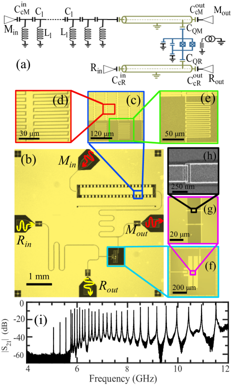
Figure 1: (a) Circuit schematic of device. (b-g) Optical micrographs of metamaterial resonator device: (b) zoomed-out image of entire chip, (c) section of metamaterial resonator containing several unit cells of inductors and capacitors, (d) detail of interdigitated capacitor, (e) detail of meander-line inductor, (f) transmon qubit with coupling capacitors to metamaterial resonator and readout resonator,(g) SQUID loop of the transmon, (h) Scanning electron microscope (SEM) image of one of the transmon junctions. (i) Transmission spectrum of metamaterial resonator measured through ports $M_{in}$ and $M_{out}$.

I Introduction

Artificial atoms formed from Josephson junction-based devices combined with linear resonant circuits are capable of reaching the strong coupling regime, where the coupling strength between the qubit and resonant microwave mode is greater than the relevant linewidths Schuster et al. (2007). The field of circuit quantum electrodynamics (cQED) Blais et al. (2004) has developed into one of the leading architectures for implementing scalable quantum processors Arute et al. (2019) while also providing a regime for exploring the light-matter interaction in microwave quantum optics with tailored artificial atoms Blais et al. (2020). For systems with multiple modes coupled to a qubit, there is the possibility of analog quantum simulation with photons in the different modes, allowing for the realization of a quantum model in a controlled platform Cirac and Zoller (2012). As one example, the light-matter interaction Hamiltonian at large coupling strengths lends itself to the realization of the spin-boson model Egger and Wilhelm (2013); Messinger et al. (2019); Leppäkangas et al. (2018); Forn-Díaz et al. (2017), a paradigmatic model of quantum dissipation and quantum phase transitions. Multi-mode cQED can also be used for studying qubit dynamics in the vicinity of photonic bandgaps Liu and Houck (2017); Mirhosseini et al. (2018), analogous to experiments using real atoms and photonic crystals Hood et al. (2016). Quantum random access memories are yet another potential application for qubits coupled to multiple modes Naik et al. (2017).

A variety of routes for achieving multi-mode cQED have been studied, including continuous transmission-line resonators Sundaresan et al. (2015) and metamaterials made from lumped circuit elements Mirhosseini et al. (2018) and Josephson junctions Kuzmin et al. (2019); Martinez et al. (2019); Hutter et al. (2011), as well as qubits coupled to acoustic and electromechanical systems Moores et al. (2018); Han et al. (2016). Lumped-element metamaterial transmission lines can be configured to tailor the band structure and thus influence the wave speed and bandgaps in the system. Possible wave dispersion properties include a left-handed dispersion relation where the mode frequency is a falling function of the wavenumber Eleftheriades et al. (2002); Caloz and Itoh (2004). Superconducting metamaterials can thus provide a low-loss system with an effective negative index of refraction Jung et al. (2014a, b). When implemented in a cQED architecture Wang et al. (2019), left-handed transmission line (LHTL) resonators provide a pathway for implementing a dense microwave mode spectrum above a low-frequency bandgap that extends down to zero frequency.

In this manuscript, we demonstrate the strong coupling of a superconducting transmon qubit Koch et al. (2007) to such a LHTL resonator. Our circuit design allows us to measure the qubit state and perform coherent qubit manipulation while separately or simultaneously driving the metamaterial resonances. We are thus able to characterize the qubit lifetime while tuning its transition frequency through the dense metamaterial mode spectrum. In addition, we can probe the Stark shift of the qubit transition due to photons in the metamaterial modes through spectroscopic measurements while driving different system resonances. We also use numerical simulations to investigate future device designs with achievable circuit parameters that can reach the regime with coupling strengths between the qubit and metamaterial modes that are larger than the intermode spacings. Our scheme thus demonstrates an approach to multimode cQED that provides a platform that can be used for quantum simulations with microwave photons or for dense quantum memories.

II Device Design and Experimental Configuration

Conventional cQED architectures involve a resonator that has a standard right-handed dispersion, where the mode frequency is an increasing function of wavenumber. Such resonators are typically formed from a distributed transmission-line segment, such as a coplanar waveguide (CPW). In principle, lumped-element implementations of the transmission-line resonator are also possible with a 1D array of series inductors and shunt capacitors to ground Pozar (2009). By contrast, building a LHTL must be done with a lumped-element metamaterial approach Eleftheriades et al. (2002). Swapping the circuit-element positions so that the array contains series capacitors $C_{l}$ with inductors $L_{l}$ to ground [Fig. 1(a)] results in a low-frequency bandgap from dc up to an infrared cutoff frequency $\omega_{IR}=1/2\sqrt{L_{l}C_{l}}$. Frequencies just above $\omega_{IR}$ correspond to the shortest wavelengths in the system, while the wavelength increases for progressively higher frequencies – a characteristic signature of left-handedness. A resonator formed from a finite-length LHTL with coupling capacitors at either end will exhibit a dense spectrum of modes just above $\omega_{IR}$ where the band is nearly flat with respect to wavenumber Wang et al. (2019).

Coupling of transmon qubits to resonant circuits is commonly achieved through a weak capacitance to a portion of the resonator near a voltage antinode of a particular mode. For a multimode system, the standing-wave pattern will in general be different for each mode. Thus, for a given qubit placement, strong coupling is only possible to the modes with large amplitudes near the qubit. For our metamaterial resonator, by building a hybrid system with one end of the LHTL connected to a right-handed transmission line (RHTL), the modes in the frequency range accessible by a typical transmon will have a short wavelength in the LH section with a much longer wavelength in the RH portion. The mode spectrum for such a hybrid LHTL-RHTL resonator still exhibits peaks near the LHTL resonances, with a slow modulation from the standing wave in the RH portion. Thus, by placing the qubit near the end of the RHTL, close to the antinodes of the low-frequency modes, the qubit can couple to all of the modes in its frequency range Egger and Wilhelm (2013).

Figure 1(a) contains a schematic of our device. The input (output) coupling capacitor $C_{cM}^{in}$ ($C_{cM}^{out}$) near the end of the LHTL (RHTL) section define the resonant modes of the hybrid transmission line structure. The transmon qubit follows the design in Ref. Chow et al. (2015) and contains a split junction allowing for the qubit transition frequency to be tuned with an external magnetic flux, which is provided by a wirewound coil above the chip. Capacitor $C_{QM}$ couples the qubit near the output end of the RHTL portion of the hybrid metamaterial; a second capacitor, $C_{QR}$, couples the qubit to a separate half-wave RHTL resonator for conventional dispersive readout of the qubit state Blais et al. (2004).

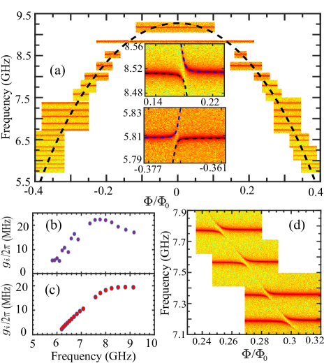
Figure 2: (a) Close-up density plot of magnitude of transmission through metamaterial resonator vs. qubit flux bias, showing vacuum Rabi splittngs for all of the modes that the qubit tunes through. Dashed line indicates flux tuning of bare transmon energy band from fits to splitting location. (Inset) closeup of splittings and fits for 5.81 GHz and 8.52 GHz modes. (b) Extracted coupling strength between qubit and each metamaterial mode vs. frequency. (c) Simulated coupling strengths vs. frequency using AWR Microwave Office and circuit model approach described in text. (d) Detail of splittings for four adjacent modes between 7.1 and 7.9 GHz.

The LHTL portion of the hybrid metamaterial resonator is fabricated from an array of 42 unit cells of series interdigitated capacitors with 29 pairs of 4-$\mu$m wide/52-$\mu$m long fingers. Between each pair of capacitors is a meander-line inductor with 9 turns of 2-$\mu$m wide traces; the inductors are arranged in a staggered pattern with alternating inductors connected to the ground plane on either side of the LHTL, as in Ref. Wang et al. (2019). The input coupling capacitor to the LHTL portion $C_{cM}^{in}$ is formed with a 4.9-$\mu$m wide gap to the input feedline. The RHTL portion of the hybrid metamaterial resonator (readout resonator) is formed from a 5-mm (7.7-mm) long CPW with a 10-$\mu$m wide center conductor and a 6-$\mu$m wide gap to the ground plane on either side. These parameters allow us to match the impedance (about 50 Ohms) between the LHTL and RHTL segments. The output end of the RHTL consists of an interdigitated capacitor $C_{cM}^{in}$ for coupling to the output feedline. (Table 2). The various circuit elements are patterned photolithographically with an etch process to define the structures in a Nb thin film on Si [Fig. 1(b-g)], with the exception of the Al-AlOx-Al Josephson junctions, which are defined with a shadow-evaporation process [Fig. 1(h)]. Further details of the fabrication and device parameters are contained in Appendices A and B.

We cool the device on a dilution refrigerator with a base temperature around 25 mK. With a vector network analyzer and microwave leads coupled to ports $M_{in}$ and $M_{out}$ [Fig. 1(b)], we measure the microwave transmission $S_{21}(f)$ and probe the modes of the LHTL-RHTL resonator [Fig. 1(h)]. The transmission below $\omega_{IR}/2\pi\approx 5\,{\rm GHz}$ is vanishingly small, followed by a dense spectrum of resonance peaks for higher frequencies. As described in Ref. Wang et al. (2019), the staggered inductor configuration of our LHTL results in the band being not quite flat at $\omega_{IR}$ so that the densest region of the spectrum is roughly 1 GHz higher than $\omega_{IR}/2\pi$.

III Probing metamaterial modes coupled to qubit

Initially we probe the qubit indirectly through transmission measurements of the hybrid metamaterial, rather than using the separate readout resonator. By varying the flux bias to tune the qubit transition frequency, we are able to observe the influence of the qubit on each mode through which it passes. The qubit has a maximum transition frequency of 9.25 GHz at an integer flux quantum ($\Phi_{0}\equiv h/2e$, where $h$ is Planck’s constant and $e$ is the electron charge) bias, thus allowing it to tune through all 21 modes below this point.

For each of these modes, when the flux bias results in the bare qubit frequency approaching a resonance, we observe a vacuum Rabi splitting Wallraff et al. (2004) in the microwave transmission where the qubit hybridizes with the photonic state of the metamaterial resonant mode [Fig. 2(a)]. Since each of these splittings is larger than the linewidth of the particular mode, this corresponds to the strong coupling regime of cQED Schuster (2007). We can fit the positions of these various splittings to the conventional transmon flux-modulation dependence Koch et al. (2007) while varying the maximum Josephson energy $E_{J0}$ to obtain the black dashed curve drawn on Fig. 2(a). The extracted value for $E_{J0}$ is consistent with the fabricated junction parameters.

Since the splittings are smaller than the intermode spacings over the range of our measurements, we can make an approximation and treat each mode individually for extracting the coupling strength $g_{i}$ for the qubit to each of the metamaterial modes. In this way, we fit each vacuum Rabi splitting to the Hamiltonian for one resonator mode coupled to a transmon. Further details on this fitting, including a discussion of the validity of treating each mode separately, are included in Appendix D. The insets to Fig. 2(a) contain two examples of these fits to the splittings while Fig. 2(b) shows a plot of the extracted $g_{i}$ values to each mode. Initially $g_{i}/2\pi$ increases with frequency above $\omega_{IR}$ up to a maximum of 22 MHz for the mode near 7.8 GHz; this is followed by a gradual decrease in $g_{i}$ up to the maximum qubit transition frequency. This non-monotonic variation of $g_{i}$ with frequency is due to the standing-wave structure in the RHTL portion of our hybrid metamaterial resonator.

For modeling $g_{i}$ and comparing with the measurements, we use AWR Microwave Office NI . We can simulate the splittings in the spectrum semi-classically by approximating the qubit as a tunable $LC$ oscillator coupled to a hybrid metamaterial resonator with the parameters of our device. Details are discussed in Appendix E. The simulated $g_{i}$ frequency dependence plotted in Fig. 2(c) is in reasonable agreement with our measured coupling strengths, although the decrease in $g_{i}$ for the highest qubit frequencies is not quite as strong. The circuit simulation allows us to explore an artificial qubit with a much higher maximum frequency so that we can study $g_{i}$ further along the metamaterial resonance spectrum. The resulting plot of $g_{i}$ vs. frequency in the Appendix E (Fig. 11) exhibits multiple dips, where the reduction that we observe in our experiment around $\sim 8-9\,{\rm GHz}$ is the first dip, due to the standing-wave structure in the RHTL portion.

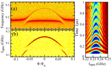
Figure 3: (a) Close-up density plot of magnitude of transmission through metamaterial resonator vs. qubit flux bias in vicinity of upper sweetspot. (b) Spectroscopy of qubit 0-1 transition vs. flux bias near the upper sweetspot measured using readout resonator. (c) Rabi spectroscopy of qubit for flux bias near upper sweet spot, around 9.235 GHz, measured using readout resonator.

In the region around 7.5 GHz, where the modes are relatively close together and the $g_{i}$ values are near the maximum, the upper branch of the splitting for one mode comes close to touching the lower branch of the splitting for the next higher mode [Fig. 2(d)]. Nonetheless, even the maximum $g_{i}$ remains smaller than the minimum mode spacing, thus, the system is not quite in the multimode strong coupling regime, where the qubit would be able to couple strongly to multiple modes simultaneously. For future devices based on this architecture, it should be possible to increase $g_{i}$ by increasing the coupling capacitance to the qubit, increasing the impedance of the metamaterial, and optimizing the length of RHTL portion of the resonator. In addition to increasing $g_{i}$, it would also be helpful to reduce the spacing between modes, which could be achieved by either increasing the number of unit cells or through appropriate engineering of the parasitic reactances. Details are discussed in Appendix VI.

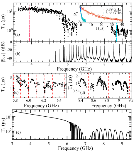
Figure 4: (a) $T_{1}$ vs. frequency measured over span of 6 GHz. (Inset) plots of two example measurements of qubit relaxation measured for a bias point below $f_{IR}$ of the metamaterial and a bias point in between two modes at higher frequencies. (b) Transmission spectrum of metamaterial resonator for comparison with structure in $T_{1}(f)$ plot. (c, d) zoomed-in $T_{1}(f)$ plots of data from (a) with red vertical dashed lines indicating location of metamaterial resonator modes. (e) Calculated $T_{1}(f)$ from multi-mode Purcell loss simulation of qubit coupled to metamaterial resonator.

IV Purcell Losses in a Multimode Environment

In addition to probing the interactions of the qubit and metamaterial modes through direct measurements of the metamaterial resonator, we are also able to read out the qubit with the separate readout resonator. By monitoring the transmission between ports $R_{in}$ and $R_{out}$ [Fig. 1(b)] with heterodyne detection, we perform conventional dispersive measurement of the qubit state. Figure 3(a) is a plot of the vacuum Rabi splittings for the highest frequency mode that the qubit passes through, observed in the microwave transmission through the metamaterial resonator between ports $M_{in}$ and $M_{out}$ with network analyzer measurements, as in the previous section. In Fig. 3(b), we use ports $R_{in}$ and $R_{out}$ to measure qubit spectroscopy in the same region of flux bias and frequency by sending a spectroscopy probe pulse at frequency $f_{spec}$, followed by a readout resonator pulse to detect the qubit-state-dependent dispersive shift. The two curves are quite similar, with comparable splittings when the bare qubit frequency passes through the 9.15 GHz mode.

We can also use the separate readout resonator for conventional coherent manipulation of the qubit state. Figure  3(c) shows a Rabi spectroscopy measurement of the qubit near its maximum transition frequency with a Rabi pulse of variable duration and frequency driven to the readout resonator, again followed by a resonator readout pulse. Thus, the qubit remains coherent in this frequency region, despite being biased in the middle of the complex resonance spectrum produced by the metamaterial resonator. A $\pi$-pulse tuned up from such a measurement allows us to excite the qubit and characterize its lifetime as it relaxes back to the ground state.

By stepping through the qubit flux bias and tuning up a $\pi$-pulse at each point, we are able to map out the qubit $T_{1}(f)$ in the structured environment of our hybrid metamaterial resonator [Fig. 4(a)]. With the qubit biased below $\omega_{IR}/2\pi$, the qubit has a reasonably long lifetime with $T_{1}$ ranging between $10-19\,\mu{\rm s}$, with a gradual decrease for larger frequencies. For frequencies near $\omega_{IR}/2\pi$ and slightly below 6 GHz, $T_{1}$ begins to drop significantly, although notably the lowest three metamaterial modes, which are particularly high Q and low transmission, do not strongly influence $T_{1}$ [Fig. 4(b)]. Beyond the fourth lowest mode, $T_{1}(f)$ is characterized by a series of sharp dips to sub-$\mu{\rm s}$ levels when the bare qubit frequency matches the various metamaterial resonances; there is a partial recovery of $T_{1}$ in between the modes [Fig. 4(c, d)]. The gap in Fig. 4(a) around 7-8 GHz is a result of the strong coupling to the readout resonator, which makes it difficult to address the qubit directly.

The complex frequency dependence of the qubit lifetime that we observe is characteristic of Purcell loss for a qubit coupled to a series of lossy resonant modes Houck et al. (2008). We note that the quality factors of the metamaterial modes in our device are entirely dominated by coupling losses to external circuitry. In this case, we chose $C_{cM}^{in/out}$ to be rather large to make it feasible to observe vacuum Rabi splittings in transmission measurements through the metamaterial while tuning the qubit frequency. For future devices, these coupling capacitances could be made significantly smaller if one were focused instead on probing the metamaterial modes via the qubit, rather than by direct transmission through the metamaterial. In this case the mode quality factors would be significantly higher and the Purcell losses much smaller, particularly when the qubit is tuned in between the modes.

Following the approach outlined in Ref. Houck et al. (2008), we model the multi-mode Purcell effect as $T_{1}^{Purcell}(f)=C/{\rm Re}[Y(f)]$, where $C$ is the qubit shunt capacitance and $Y(f)$ is the frequency-dependent complex admittance of the qubit environment. We obtain $Y(f)$ using the circuit model of the impedance of a LHTL that we derived previously in Ref. Wang et al. (2019) combined with the standard expression for a RHTL. Additionally we include a non-Purcell term $T_{1}^{non-Purcell}(f)\propto 1/f$ to model the effects of dielectric loss with a frequency-independent loss tangent that is typically observed in frequency-tunable transmons Barends et al. (2013); Hutchings et al. (2017). Further details of the $T_{1}(f)$ modeling are described in Appendix F. The resulting $T_{1}(f)$ dependence from our model plotted in Fig. 4(e) qualitatively follows our measurements, although we do not quantitatively reproduce the locations of the $T_{1}$ dips due to the difficulty of capturing the experimental metamaterial spectrum in our circuit model, particularly near $\omega_{IR}/2\pi$, without accounting for the effects of the staggered inductor configuration and non-ideal grounding of the metamaterial chip, as described in Ref. Wang et al. (2019). Nonetheless, the Purcell modeling provides a route for describing the frequency-dependent lifetime for a qubit coupled to a complex metamaterial, including the relatively long $T_{1}$ values that can be attained in the bandgap of the metamaterial spectrum.

V Stark Shift Measurements

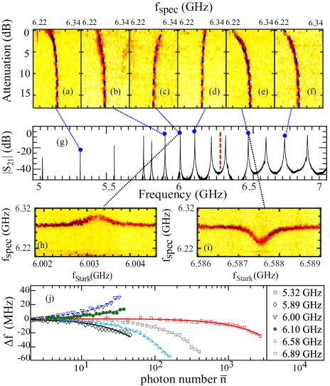
Figure 5: (a-f) Stark shifts of qubit transition through driving of 6 different metamaterial modes at a range of microwave powers for a flux bias corresponding to the unshifted qubit transition at 6.275 GHz; Stark shift theoretical curves shown by blue dashed lines. For the 6 plots, 0 dB attenuation corresponds to a power at the chip of (a) -86 dBm, (b) -126 dBm, (c) -128 dBm, (d) -123 dBm, (e) -121 dBm, and (f) -113 dBm. (g) $|S_{21}(f)|$ measured through metamaterial to indicate the 6 modes driven in (a-f) (blue dots and dotted lines) and the bias point of the qubit (red dashed line). Plots of qubit spectroscopy frequency vs. Stark drive frequency for fixed power for (h) mode near 6.003 GHz at -129 dBm, (i) mode near 6.588 GHz at -122 dBm; metamaterial mode near 6.22 GHz visible as a faint, sharp line near bottom of plots. (j) Extracted Stark shifts in qubit transtion frequency from (a-f) plotted vs. mean photon number for each of the 6 metamaterial modes, as described in text.

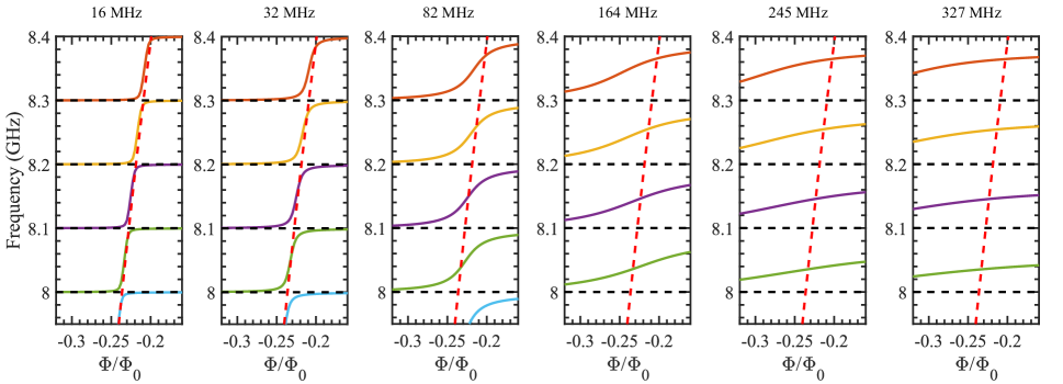
Figure 6: Numerical solutions for a transmon coupled to four modes with 100 MHz intermode spacing; bare mode frequencies are indicated by horizontal dashed lines. Nearly vertical red dashed line corresponds to bare transmon frequency. Label at the top of each plot indicates the coupling strength $g_{i}/2\pi$ between each of the four modes and the transmon.

With the ability to perform dispersive measurements of the qubit with the readout resonator (using $R_{in/out}$) while simultaneously driving a separate microwave signal to the hybrid metamaterial resonator (using $M_{in/out}$), we are able to observe the ac Stark shift of the qubit 0-1 transition Schuster et al. (2005) for different average numbers of photons in each of the metamaterial modes. With the qubit biased at 6.275 GHz, as indicated in Fig. 5(g), we measure the qubit transition in spectroscopy while driving one of the six different metamaterial modes and scanning over 18 dB of power for the Stark drive to generate the plots in Fig. 5(a-f). Additionally, for two of these metamaterial modes, we again perform qubit spectroscopy while scanning the frequency of the Stark drive for fixed power [Fig. 5(h,i)].

The observed shift of the qubit transition increases in magnitude with the power of the Stark drive when the frequency is resonant with a metamaterial mode, as with a qubit coupled to a single resonator Schuster et al. (2005). Moreover, if the metamaterial mode being driven falls between the qubit 0-1 and 1-2 transition frequencies, the straddling regime identified in Ref. Koch et al. (2007), we observe a change in the sign of the Stark shift. The observed Stark shifts of the qubit with microwave driving of various metamaterial modes can be explained well by a model of a transmon qubit coupled dispersively to a single mode resonator, corresponding to the particular mode being driven (mode $i$), according to

$$H/\hbar=\omega_{i}\hat{\mathbb{M}_{i}}+\left(\frac{\omega_{q}}{2}+\chi\hat{\mathbb{M}_{i}}\right)\sigma_{z},$$ (1)

where $\omega_{i}$ is the frequency of the relevant (single) metamaterial mode, $\hat{\mathbb{M}_{i}}=\sum_{m_{i}}m_{i}|m_{i}\rangle\langle m_{i}|$ is the number operator for mode $i$, $\omega_{q}$ is the qubit 0-1 transition frequency, $\chi=g_{i}^{2}\eta/(\delta_{i}\eta-\delta_{i}^{2})$ is the qubit frequency shift per photon, $\delta_{i}=\omega_{q}-\omega_{i}$ is the detuning between the qubit and the metamaterial mode, and $\eta$ is the anharmonicity of the transmon, defined as the difference between the 1-2 and 0-1 transition frequencies. The Stark tone at frequency $\omega_{d}$ drives the resonator to a coherent steady state with average photon number

$$\bar{n}_{i}=\langle\hat{\mathbb{M}_{i}}\rangle=\frac{\Omega_{i}^{2}}{(\omega_{i}-\omega_{d})^{2}+\frac{\kappa^{2}_{i}}{4}}.$$ (2)

Here, $\Omega_{i}$ is the effective drive amplitude for mode $i$ and and $\kappa_{i}$ is the mode decay rate from separate measurements of the linewidth of each metamaterial mode (Fig. 10). Thus, $\bar{n}_{i}$ is proportional to the power delivered to the mode. Making a semiclassical approximation to the Hamiltonian in Eq. (1), one finds the qubit Stark shift to be given by $\chi\bar{n}_{i}$. A single-parameter linear fit between the power measured at the chip for each mode frequency from a separate baseline cooldown and the observed Stark shift for each driven mode gives a map from the input drive power for each mode and the actual power delivered to the mode, $\Omega_{i}^{2}$. This fit parameter then allows us to compute the theory curves included in Fig. 5.

VI Approaches for increasing qubit-metamaterial mode couplings

Although on our present device the coupling strength between the qubit and each metamaterial mode was always less than the spacing between modes $\Delta\omega_{i}$, in this section we consider the parameters for a hypothetical qubit-metamaterial device that could reach superstrong coupling Kuzmin et al. (2019), where $g_{i}/\Delta\omega_{i}>1$. In this regime, the qubit can be strongly coupled to multiple modes simultaneously. When combined with the ability to perform fast, non-adiabatic manipulation of the qubit transition frequency, this could be used to prepare multi-mode entangled states of photons over a range of metamaterial modes Egger and Wilhelm (2013). In this section, we consider various modifications to the metamaterial and qubit, some of which enhance $g_{i}$ and others that decrease $\Delta\omega_{i}$.

Table 1: Modified metamaterial parameters for hypothetical device with enhanced coupling strength used in AWR simulation.

Label	Description	Value for	New value
		measured chip
$N_{l}$	Number of LHTL unit cells	42	82
$Z_{M}$	Metamaterial impedance	50 $\Omega$	200 $\Omega$
$N_{r}$	Number of RHTL unit cells	N/A	20
$L_{RH}$	RHTL unit cell inductance	N/A	0.35 nH
$C_{RH}$	RHTL unit cell capacitance	N/A	9.5 fF
$C_{QM}$	Qubit-metametarial	4.3 fF	50 fF
	coupling capacitance
$C_{Q}$	Qubit capacitance	48 fF	50 fF

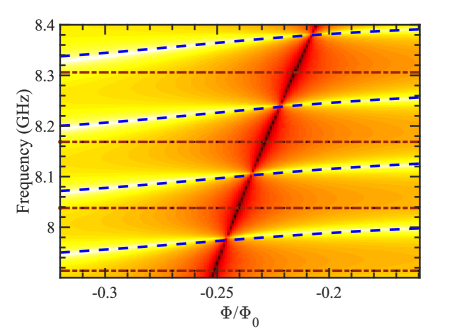
Figure 7: Simulation of hypothetical qubit-metamaterial device to achieve superstrong coupling through AWR circuit simulation of device described in text using parameters in Table 1 and numerical solution to Hamiltonian (blue dashed lines) with adjusted coupling strength values to match features in AWR simulation. Black dotted line corresponds to bare qubit transition frequency. The brown horizontal dashed-dotted lines show the bare frequencies for each of the four modes, 7.91 GHz, 8.04 GHz, 8.17 GHz, and 8.31 GHz, with extracted $g_{i}/2\pi$ values 220 MHz, 193 MHz, 180 MHz, and 178 MHz, respectively.

One approach for increasing $g_{i}$ involves increasing $C_{QM}$, as $g_{i}\propto C_{QM}/C_{\Sigma}^{1/2}$ [2]. We note that large coupling strengths between a qubit and resonator can also be achieved through inductive coupling Niemczyk et al. (2010), but for now, we will restrict our design considerations to capacitive coupling. Another route for enhancing $g_{i}$ involves increasing the impedance of the metamaterial resonator. For the LHTL portion, this is straightforward to achieve by adjusting the values of $L_{l}$ and $C_{l}$. However, making a significant increase in the impedance for the RHTL portion is difficult with a CPW configuration. For example, a CPW impedance of 120 $\Omega$ requires a center conductor width of 500 nm and a 10-$\mu{\rm m}$ gap to the ground plane, which can be challenging to fabricate. As an alternative, we consider using a lumped-element implementation for the RHTL portion, which allows for larger impedances by choosing the inductor and capacitor values appropriately. We note that a lumped-element RHTL is a departure from our present design, but this should not introduce any complications since our device layout already includes chains of similar lumped-element inductors and capacitors for the LHTL and these would all get fabricated at the same time. In addition to increasing the coupling capacitance and resonator impedance, the length of the RHTL portion also impacts the coupling strength through the variation of the standing-wave amplitude at the location of the qubit. Besides increasing $g_{i}$, we can also decrease $\Delta\omega_{i}$ by adding more unit cells to the LHTL or by using a superlattice arrangement for the LHTL Messinger et al. (2019), both of which increase the mode density since the number of modes between the IR and UV cutoff frequencies corresponds to the number of unit cells. Table 1 summarizes the various parameters for our hypothetical qubit-metamaterial device capable of achieving $g_{i}/\Delta\omega_{i}>1$.

With the parameters of our hypothetical device described above, we characterize the coupling by simulating the microwave transmission through the metamaterial while tuning the qubit frequency. In order to build intuition about the splittings in the spectrum for the superstrong coupling regime, we also study the system Hamiltonian [presented in Appendix D, Eq. (3)] for various values of $g_{i}$. Because the size of the Hilbert space grows exponentially with the number of modes, in order to keep the numerical simulation tractable, we restrict the system to four modes spaced by 100 MHz for the simulations shown in Fig. 6. For small $g_{i}$, such as the 16 MHz and 32 MHz plots, the solutions exhibit conventional vacuum Rabi splittings as the qubit passes through each of the individual metamaterial modes. For larger $g_{i}$, the splitting from one mode begins to merge with the splitting from the next mode, and by the point with 164 MHz couplings, the splittings become difficult to distinguish from the strongly shifted modes.

Figure 7 contains a 500-MHz segment of the simulated transmission spectrum for our hypothetical device with the parameters from Table 1 as a function of the qubit flux. We then run a numerical solution to the system Hamiltonian with four modes, corresponding to the bare mode frequencies in the frequency window of Fig. 7, and adjust the coupling strengths $g_{i}$ in the Hamiltonian for these four modes to match the features in the AWR simulation. The blue dashed lines follow the Hamiltonian solutions and correspond to coupling strengths of between 178-220 MHz. Thus, $g_{i}/\Delta\omega_{i}$ ranges between 1.28 and 1.84, so that the hypothetical device with experimentally feasible parameters is capable of reaching the superstrong multimode coupling regime.

VII Conclusions

In conclusion, we have demonstrated strong coupling of a transmon qubit to a metamaterial transmission line resonator. The left-handed dispersion of the structure resulted in a dense mode spectrum within the tuning window of the qubit transition frequency. We studied the influence of the metamaterial resonances on the qubit dynamics through measurements of energy relaxation and the ac Stark shift with different numbers of photons in several of the modes. As discussed in Sec. VI, there is a straightforward path for a future device design that can enter the superstrong coupling regime Kuzmin et al. (2019), where the coupling strength is larger than the mode spacing.

While the present sample was not configured for fast modulation of the qubit frequency, a future device could be designed with an on-chip flux-bias line for fast qubit tuning. This could enable new experiments with the qubit pulsed quickly between operating points below the metamaterial bandgap and resonance with different metamaterial modes Hofheinz et al. (2008); alternatively, for such a device the qubit could be parametrically modulated at the sideband frequency between the qubit transition and a particular metamaterial mode Strand et al. (2013); Naik et al. (2017). Both approaches could be used for swapping excitations between the qubit and the metamaterial. Such capabilities would allow for the preparation of complex multi-mode photonic states in the metamaterial that could be used for analog quantum simulations with microwave photons Egger and Wilhelm (2013); Messinger et al. (2019), which could be made to interact through the nonlinearity coupled from the qubit when biased near the mode frequencies. Additionally, this system could be used for a quantum storage with microwave excitations in different metamaterial modes serving as memory elements.

VIII Acknowledgments

We acknowledge useful discussions with Jaseung Ku and assistance with device fabrication from JJ Nelson. This work is supported by the U.S. Government under ARO Grants No. W911NF-14-1-0080 and No. W911NF-15-1-0248. Device fabrication is performed at the Cornell NanoScale Facility, a member of the National Nanotechnology Infrastructure Network, which is supported by the National Science Foundation (Grant NNCI-2025233). B.G.T. acknowledges support from CNPq INCT-IQ (465469/2014-0) and Coordenação de Aperfeiçoamento de Pessoal de Nível Superior - Brasil (CAPES) - Finance Code 001.

Appendix A Fabrication Details

The device was fabricated with two lithographic steps. Initially an 80-nm thick Nb film was sputter deposited onto a high-resistivity Si wafer. All of the circuit elements besides the qubit junctions were then patterned in a single photolithography step with UVN2300 deep-UV negative resist. After development, the pattern was etched using an inductively coupled plasma etcher with BCl₃, Cl₂, and Ar. Next, the transmon junctions were defined with an electron-beam lithography step and a bilayer of MMA and PMMA to form the junction electrodes and airbridge for shadow evaporation. Following development in methyl isobutyl ketone, the junctions were formed by double-angle depostion of Al thin films with 35 nm for the first layer and 65 nm for the second layer. The tunnel barriers were formed by an in situ oxidation step in between the two film depositions; the unwanted Al was lifted off using dichloromethane following the vacuum step.

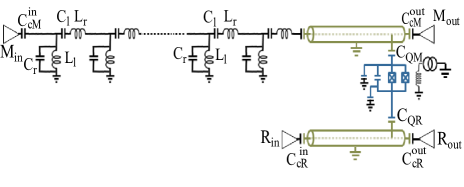
Figure 8: Circuit schematic of the device, including stray reactances.

Table 2: Metamaterial parameters determined by finite element simulations of circuit layout.

Label	Description	Value
$L_{l}$	Unit cell inductance	0.7 nH
$C_{l}$	Unit cell capacitance	250 fF
$L_{r}$	Unit cell stray inductance	0.03 nH
$C_{r}$	Unit cell stray capacitance	25 fF
$C_{cM}^{in}$	Metamaterial input	30 fF
	coupling capacitor
$C_{cM}^{out}$	Metamaterial output	25 fF
	coupling capacitor

Appendix B Metamaterial and Qubit Parameters

Table 2 lists the metamaterial parameters, which were determined by finite element simulations. In order to account for stray reactances, we include parasitic series inductors $L_{r}$ and shunt capacitors $C_{r}$ in each unit cell (Fig. 8) with parameters extracted from related structures that we modeled previously in Ref. Wang et al. (2019).

Figure 9 compares the measured transmission spectrum for the hybrid metamaterial with a circuit simulation of $S_{21}(f)$ using AWR Microwave Office with the parameters in the table. The spectra are reasonably close, with the most significant deviation at the low-frequency end, where the measured device has a softer infrared cutoff due to the staggered inductor configuration, as discussed in Ref. Wang et al. (2019). Figure 10 shows the total quality factor of modes extracted by Lorentzian fits to measured spectrum as function of frequency. Note that the quality factors for these modes are entirely dominated by coupling losses to external circuitry through the coupling capacitances.

Table 3 lists the qubit and readout resonator parameters, as determined by a combination of low-temperature measurements and circuit simulations.

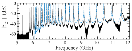
Figure 9: Measured transmission spectrum (black line) compared with spectrum from circuit simulation using AWR (blue dashed line).

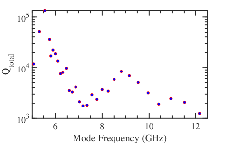
Figure 10: Total quality factor of metamaterial modes as function of frequency. The presence of the RHTL segment that is used to couple the metamaterial to the qubit results in the non-monotonic behavior of the mode quality factor vs. frequency through the variation in the standing wave pattern in the RHTL portion with frequency; by contrast, a simple LHTL resonator exhibits a monotonic decrease in quality factor for increasing frequencyWang et al. (2019).

Table 3: Qubit and readout resonator parameters.

Label	Description	Value	Method of Determination
$f_{01}^{max}$	Maximum qubit frequency	9.25 GHz	Qubit spectroscopy of the $f_{01}$ transition
			at the flux-insensitive sweetspot
$C_{Q}$	Qubit shunt capacitance	48 fF	Finite element simulations
$g_{R}/2\pi$	Qubit-readout resonator	65 MHz	Measurement of resonator
	coupling strength		transmission $S_{21}$ vs. flux
$\omega_{R}/2\pi$	Fundamental frequency of	7.07 GHz	Measurement of resonator
	readout resonator		transmission $S_{21}$
$Q$	Total quality factor of	15,463	Measurement of resonator
	readout resonator		transmission $S_{21}$
$C_{cR}^{in}$	Readout resonator input	1 fF	Finite element simulations
	coupling capacitor
$C_{cR}^{out}$	Readout resonator output	2 fF	Finite element simulations
	coupling capacitor
$C_{QR}$	Qubit-readout resonator	4.8 fF	Finite element simulations
	coupling capacitor
$C_{QM}$	Qubit-metametarial	4.3 fF	Finite element simulations
	coupling capacitor
$C_{J}$	Junction capacitance	2.5 fF	Junction area from SEM image

Appendix C Measurement setup

The device was diced into a $6.25\times 6.25\,{\rm mm}^{2}$ chip and wire-bonded into a machined aluminum sample box and covered by a lid with an integrated superconducting wirewound coil. The sample box was mounted on the cold finger of a dilution refrigerator with a base temperature around 25 mK and was shielded by a single-layer cryogenic magnetic shield. The input coaxial lines to the metamaterial and readout resonator inputs each had 50 dB of cold attenuation as well as 12 GHz low-pass filters. The output lines also had 12 GHz low-pass filters before passing through a microwave relay switch, followed by a series of microwave isolators on the millikelvin stage. The output amplification consisted of a HEMT amplifier at 4 K plus 35 dB of room-temperature amplification. A room-temperature $\mu$-metal magnetic shield was used around the vacuum jacket of the dilution refrigerator.

Appendix D Extraction of qubit-metamaterial mode couplings from spectra

In order to determine the coupling strength $g_{i}$ between the transmon and mode $i$ of the metamaterial with frequency $\omega_{i}$, we assume each mode can be represented as an independent harmonic oscillator coupled capacitively to the transmon. We then utilize standard circuit quantization Koch et al. (2007); Egger and Wilhelm (2013) to derive the Hamiltonian for the transmon-coupled metamaterial, which, when written in the basis of transmon charge $|n\rangle$ and resonator excitation number $|m_{i}\rangle$ is given by

$$\begin{split}\hat{H}=\left[\sum_{n}\left(4E_{C}(n-n_{g})^{2}|n\rangle\langle n|-\frac{E_{J}}{2}\left(|n+1\rangle\langle n|+|n\rangle\langle n+1|\right)\right)\right]\otimes\hat{\mathbb{I}}_{m}+\\ \sum_{i}\left[\sum_{m_{i}}\hat{\mathbb{I}}_{n}\otimes\hbar\omega_{i}\left(|m_{i}\rangle\langle m_{i}|+\frac{1}{2}\right)+\sum_{n,m_{i}}\hbar g_{i}n|n\rangle\langle n|\otimes\sqrt{m_{i}+1}(|m_{i}+1\rangle\langle m_{i}|+|m_{i}\rangle\langle m_{i}+1|)\otimes\hat{\mathbb{I}}_{m_{j\neq i}}\right].\end{split}$$ (3)

Here, $\hat{\mathbb{I}}_{m}$ is the product of metatmaterial mode identity operators, $\hat{\mathbb{I}}_{m_{i}}$ is the identity operator for metamaterial mode $i$, $\hat{\mathbb{I}}_{n}$ is the charge basis identity operator, $E_{C}=e^{2}/2C_{\Sigma}$ where $(C_{\Sigma}=C_{Q}+2C_{J}+C_{QR}+C_{QM})$ is the transmon charging energy, $n_{g}$ is the transmon polarization charge, and $E_{J}$ is the flux-tunable Josephson energy, which, for the case of symmetric junctions, is given by

$$E_{J}=E_{J0}\left|\cos\left(\pi\frac{\Phi}{\Phi_{0}}\right)\right|,$$ (4)

where $E_{J0}$ is the maximum Josephson energy, $\Phi$ is the external flux applied to the transmon, and $\Phi_{0}\equiv h/2e$ is the flux quantum. For our device, $E_{C}/h=0.31$ GHz and $E_{J0}/h=37$ GHz. Note that due to the large ratio of $E_{J}/E_{C}$ and the level of uniformity achieved in the Josephson junction fabrication, the dependence on $n_{g}$ and junction asymmetry are assumed to be negligible in the model for the fitting routine discussed below.

Next, we implement a numerical minimization routine in Matlab to fit the lowest two eigenvalues of the model Hamiltonian to the frequency response of metamaterial transmission measurements versus flux $\Phi$ (main text, Fig. 2(a) and inset) in the vicinity of each vacuum Rabi splitting. For each fit, we truncate the transmon Hilbert space to 21 charge states and each resonator mode to 4 number states. In order to reduce the convergence time of the fit to an acceptable duration, for each vacuum-Rabi splitting $i$, we include just a single metamaterial mode in the model (i.e., mode $i$ with frequency $\omega_{i}$). Note that in each fit, $g_{i}$ is the only free parameter, with all other parameters in the Hamiltonian determined via independent measurements. In several trial cases, to estimate the error that results from neglecting the full spectrum of metamaterial modes, we performed fits where we solved the Hamiltonian including two nearest neighbor modes, rather than only one mode. We found the extracted value of each $g_{i}$ in these cases to be within 5% of the value from the fits with only a single metamaterial mode. This is compatible with the coupling regime for our present device, where $g_{i}$ remains less than the intermode spacing $\Delta\omega_{i}$ between modes $i$ and $i+1$ over the range of our measurements..

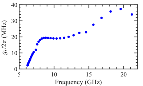
Figure 11: Simulated $g_{i}$ from AWR/circuit model extended out to higher frequency for a hypothetical qubit with higher upper sweetspot. The slight deviation at 7.5 GHz and 15 GHz is due to mode frequency approaching fundamental and first harmonic modes of readout resonator.

Appendix E Calculation of qubit-metamaterial mode couplings

For modeling $g_{i}$, the coupling between metamaterial mode $i$ and the transmon qubit, we use a semi-classical approach involving the AWR Microwave Office circuit simulator NI . Note, all the circuit parameters used in the simulation are listed in Tables 2 and 3. As shown in Fig. 8, the LHTL section of the metamaterial resonator consists of 42 unit cells of series capacitors $C_{l}$ and inductors $L_{l}$ to ground, as in the measured device. In addition, we include parasitic effects in each cell consisting of a small lumped-element inductor $L_{r}$ in series with $C_{l}$ that accounts for the stray inductance of the interdigitated capacitor; a small lumped-element capacitor $C_{r}$ in parallel with $L_{l}$ accounts for the stray capacitance from the meander-line inductors. The values for these circuit parameters used in the simulations were chosen based on our earlier modeling of LHTL resonators Wang et al. (2019), including simulations with Ansys Q3D ANSYS and Sonnet Sonnet . We set the loss in the capacitors in AWR to correspond to an internal quality factor of $10^{5}$ Wang et al. (2019).

For the AWR modeling, we treat the transmon as a tunable, lumped-element $LC$ oscillator, with $L$ being flux-tunable and the $L$ and $C$ values determined by the measured device. The coupling between the qubit and the RHTL CPW portion of the metamaterial resonator is set by the coupling capacitor $C_{QM}$, as listed in Table 3. The simulation also includes the separate CPW readout resonator (Fig. 8), using parameters corresponding to the measured device, with coupling capacitor $C_{QR}$ to the qubit.

To extract the value of $g_{i}$, we simulate $S_{21}$ transmission measurements through the metamaterial (i.e., between $M_{in}$ and $M_{out}$ in Fig. 8). We adjust $L$ for the qubit to simulate flux tuning and bring the qubit near resonance with mode $i$. We then scan the qubit $L$ to sweep it through resonance with mode $i$, and thus generate a simulated vacuum Rabi splitting. We thus determine the coupling strength to mode $i$ from the minimum spacing in the avoided-level crossing with the qubit, corresponding to twice the simulated coupling strength, $2g_{i}$. With this technique, we can simulate the frequency dependence of $g_{i}$ vs. mode frequency $\omega_{i}$, as in Fig. 2(c) of the main manuscript.

Unlike our measured device, where the upper sweet spot of the qubit is 9.25 GHz, the circuit simulations allow us to explore an artificial qubit with a much higher maximum frequency, so that we can study $g_{i}$ further along the metamaterial resonance spectrum. The plot in Fig. 11 exhibits multiple dips as the mode frequencies increase, which are due to the standing-wave structure in the RHTL portion. As the standing-wave pattern in the RHTL portion changes, the voltage level coupled to the qubit through $C_{QM}$, and hence the coupling strength $g_{i}$, can change.

Appendix F Calculation of Purcell loss

The complex frequency dependence of the qubit lifetime that we observe in Fig. 4 can be described by a combination of Purcell loss for a qubit coupled to a series of lossy resonant modes Houck et al. (2008) and dielectric loss with a frequency-independent loss tangent that is typically observed in frequency-tunable transmons Barends et al. (2013); Hutchings et al. (2017):

$$\frac{1}{T_{1}}=\frac{1}{T_{1}^{Purcell}}+\frac{1}{T_{1}^{non-Purcell}},$$ (5)

where $T_{1}^{non-Purcell}(\omega)=A/\omega$ for some constant $A$. This, of course, is a simplification, as even simple real devices with a single qubit coupled to a single resonator mode can exhibit structure in a measurement of $T_{1}(\omega)$ as the qubit passes through strongly coupled two-level system (TLS) or other spurious resonances at various frequencies Barends et al. (2013). Nonetheless, this gives us a starting point for modeling the frequency dependence of $T_{1}$ on our device.

Following the approach outlined in Ref. Houck et al. (2008), we model the multi-mode Purcell effect as

$$T_{1}^{Purcell}(\omega)=(C_{Q}+2C_{J})/{\rm Re}[Y(\omega)],$$ (6)

where $C_{Q}$ is the qubit shunt capacitance, $C_{J}$ is the single junction capacitance, and $Y(\omega)$ is the frequency-dependent complex admittance of the qubit environment. By modeling $Y(\omega)$ for our qubit environment and computing $T_{1}$ from Eqs. (5, 6), we are able to compute the multi-mode Purcell loss curve in Fig. 4(e). The environment for our qubit consists of the impedance of the readout resonator coupled to the qubit $Z_{R}(\omega)$ and the hybrid metamaterial resonator coupled to the qubit $Z_{M}(\omega)$: $Y(\omega)=1/Z_{R}(\omega)+1/Z_{M}(\omega)$. From the coupling to the readout resonator, we have:

$${Z_{R}(\omega)}=\frac{1}{i\omega C_{QR}}+\frac{1}{\frac{1}{Z_{RA}}+\frac{1}{Z_{RB}}},$$ (7)

where $Z_{RA}$ and $Z_{RB}$ are the impedances of the two segments of the readout resonator on either side of the coupling element with length $l_{A}=$ 6.88 mm and $l_{B}=$ 0.792 mm, respectively, and given by the standard expression from Ref. Pozar (2009):

$$Z_{RA}(\omega)=Z_{0}\frac{Z_{LA}+iZ_{0}\tanh(\gamma l_{A})}{Z_{0}+iZ_{LA}\tanh(\gamma l_{A})},$$ (8)

where $Z_{0}=50\,\Omega$ is the characterstic impedance of the readout resonator transmission line, $Z_{LA}=1/i\omega C_{cR}^{in}+R_{0}$ and $R_{0}$ is the source impedance on the input line, which is also 50 $\Omega$; $\gamma=\alpha+i\beta$ is the propagation constant, where $\alpha=10^{-5}\pi/2l_{A}$ accounts for internal transmission line losses; $\beta=\omega\sqrt{\epsilon}/c$, where $\epsilon$ is the effective relative permittivity for the transmission line and $c$ is the speed of light. We get a similar expression for $Z_{RB}(\omega)$, except $Z_{LB}=1/i\omega C_{cR}^{out}+R_{0}$.

The impedance coupled to the qubit by the metamaterial resonator is given by

$${Z_{M}(\omega)}=\frac{1}{i\omega C_{QM}}+\frac{1}{\frac{1}{Z_{MA}}+\frac{1}{Z_{MB}}},$$ (9)

where $Z_{MA}$ is the impedance of the RHTL segment of length 0.9 mm between the coupling point of the qubit along the RHTL and the output coupling capacitor of the metamaterial, which is described by a similar expression to Eq. (8) with $Z_{L}=1/i\omega C_{cM}^{out}+R_{0}$; $Z_{MB}$ is the series impedance of the LHTL line and RHTL segment of length 4 mm.

$${Z_{MB}(\omega)}=Z_{0r}\frac{Z_{LHTL}+iZ_{0r}\tanh(\gamma l)}{Z_{0r}+iZ_{LHTL}\tanh(\gamma l)},$$ (10)

where $Z_{0r}$ is again 50 $\Omega$ and $\gamma$ is the same as discussed previously following Eq. (8); $Z_{LHTL}$ represents the impedance of a LHTL with $N$ unit cells and unit cell length $\Delta x$, which we derived previously in Ref. Wang et al. (2019):

$$Z_{LHTL}=Z_{0l}\frac{e^{ikN\Delta x}+\Gamma e^{-ikN\Delta x}}{e^{-ik(-N+\frac{1}{2})\Delta x}-\Gamma e^{ik(-N+\frac{1}{2})\Delta x}},$$ (11)

with reflection coefficient

$$\Gamma=\frac{Z_{s}e^{\frac{-ik\Delta x}{2}}-Z_{0l}}{Z_{s}e^{\frac{ik\Delta x}{2}}+Z_{0l}},$$ (12)

and input impedance

$$Z_{s}=1/i\omega C^{in}_{cM}+R_{0},$$ (13)

where $R_{0}$ is the source impedance connected to the LHTL input; the characteristic impedance is given by

$$Z_{0l}=\left.\left(i\omega L_{r}+\frac{1}{i\omega C_{l}}\right)\middle/2i\sin(k\Delta x/2)\right.,$$ (14)

and the wavenumber $k$ can be obtained from the LHTL dispersion relation

$$k(\omega)\Delta x=\cos^{-1}\left[1-\frac{1}{2}\left(\omega L_{r}-\frac{1}{\omega C_{l}}\right)\left(\omega C_{r}-\frac{1}{\omega L_{l}}\right)\right].$$ (15)

References

- Schuster et al. (2007) D. I. Schuster, A. A. Houck, J. A. Schreier, A. Wallraff, J. M. Gambetta, A. Blais, L. Frunzio, J. Majer, B. Johnson, M. H. Devoret, S. M. Girvin, and R. J. Schoelkopf, Resolving photon number states in a superconducting circuit, Nature 445, 515 (2007).
- Blais et al. (2004) A. Blais, R.-S. Huang, A. Wallraff, S. M. Girvin, and R. J. Schoelkopf, Cavity quantum electrodynamics for superconducting electrical circuits: An architecture for quantum computation, Phys. Rev. A 69, 062320 (2004).
- Arute et al. (2019) F. Arute, K. Arya, R. Babbush, D. Bacon, J. C. Bardin, R. Barends, R. Biswas, S. Boixo, F. G. Brandao, D. A. Buell, B. Burkett, Y. Chen, Z. Chen, B. Chiaro, R. Collins, W. Courtney, A. Dunsworth, E. Farhi, B. Foxen, A. Fowler, C. Gidney, M. Giustina, R. Graff, K. Guerin, S. Habegger, M. P. Harrigan, M. J. Hartmann, A. Ho, M. Hoffmann, T. Huang, T. S. Humble, S. V. Isakov, E. Jeffrey, Z. Jiang, D. Kafri, K. Kechedzhi, J. Kelly, P. V. Klimov, S. Knysh, A. Korotkov, F. Kostritsa, D. Landhuis, M. Lindmark, E. Lucero, D. Lyakh, S. Mandrà, J. R. McClean, M. McEwen, A. Megrant, X. Mi, K. Michielsen, M. Mohseni, J. Mutus, O. Naaman, M. Neeley, C. Neill, M. Y. Niu, E. Ostby, A. Petukhov, J. C. Platt, C. Quintana, E. G. Rieffel, P. Roushan, N. C. Rubin, D. Sank, K. J. Satzinger, V. Smelyanskiy, K. J. Sung, M. D. Trevithick, A. Vainsencher, B. Villalonga, T. White, Z. J. Yao, P. Yeh, A. Zalcman, H. Neven, and J. M. Martinis, Quantum supremacy using a programmable superconducting processor, Nature 574, 505 (2019).
- Blais et al. (2020) A. Blais, S. M. Girvin, and W. D. Oliver, Quantum information processing and quantum optics with circuit quantum electrodynamics, Nat. Phys. 16, 247 (2020).
- Cirac and Zoller (2012) J. I. Cirac and P. Zoller, Goals and opportunities in quantum simulation, Nat. Phys. 8, 264 (2012).
- Egger and Wilhelm (2013) D. J. Egger and F. K. Wilhelm, Multimode circuit quantum electrodynamics with hybrid metamaterial transmission lines, Phys. Rev. Lett. 111, 163601 (2013).
- Messinger et al. (2019) A. Messinger, B. G. Taketani, and F. K. Wilhelm, Left-handed superlattice metamaterials for circuit QED, Phys. Rev. A 99, 032325 (2019).
- Leppäkangas et al. (2018) J. Leppäkangas, J. Braumüller, M. Hauck, J.-M. Reiner, I. Schwenk, S. Zanker, L. Fritz, A. V. Ustinov, M. Weides, and M. Marthaler, Quantum simulation of the spin-boson model with a microwave circuit, Phys. Rev. A 97, 052321 (2018).
- Forn-Díaz et al. (2017) P. Forn-Díaz, J. J. García-Ripoll, B. Peropadre, J. L. Orgiazzi, M. A. Yurtalan, R. Belyansky, C. M. Wilson, and A. Lupascu, Ultrastrong coupling of a single artificial atom to an electromagnetic continuum in the nonperturbative regime, Nat. Phys. 13, 39 (2017).
- Liu and Houck (2017) Y. Liu and A. A. Houck, Quantum electrodynamics near a photonic bandgap, Nat. Phys. 13, 48 (2017).
- Mirhosseini et al. (2018) M. Mirhosseini, E. Kim, V. S. Ferreira, M. Kalaee, A. Sipahigil, A. J. Keller, and O. Painter, Superconducting metamaterials for waveguide quantum electrodynamics, Nat. Commun. 9, 3706 (2018).
- Hood et al. (2016) J. D. Hood, A. Goban, A. Asenjo-Garcia, M. Lu, S.-P. Yu, D. E. Chang, and H. J. Kimble, Atom–atom interactions around the band edge of a photonic crystal waveguide, Proc. Natl. Acad. Sci. 113, 10507 (2016).
- Naik et al. (2017) R. Naik, N. Leung, S. Chakram, P. Groszkowski, Y. Lu, N. Earnest, D. McKay, J. Koch, and D. Schuster, Random access quantum information processors using multimode circuit quantum electrodynamics, Nat. Commun. 8, 1904 (2017).
- Sundaresan et al. (2015) N. M. Sundaresan, Y. Liu, D. Sadri, L. J. Szöcs, D. L. Underwood, M. Malekakhlagh, H. E. Türeci, and A. A. Houck, Beyond strong coupling in a multimode cavity, Phys. Rev. X 5, 021035 (2015).
- Kuzmin et al. (2019) R. Kuzmin, N. Mehta, N. Grabon, R. Mencia, and V. E. Manucharyan, Superstrong coupling in circuit quantum electrodynamics, npj Quant. Inform. 5, 20 (2019).
- Martinez et al. (2019) J. P. Martinez, S. Leger, N. Gheeraert, R. Dassonneville, L. Planat, F. Foroughi, Y. Krupko, O. Buisson, C. Naud, W. Guichard, S. Florens, I. Snyman, and N. Roch, A tunable Josephson platform to explore many-body quantum optics in circuit-QED, npj Quant. Inform. 5, 19 (2019).
- Hutter et al. (2011) C. Hutter, E. A. Tholén, K. Stannigel, J. Lidmar, and D. B. Haviland, Josephson junction transmission lines as tunable artificial crystals, Phys. Rev. B 83, 014511 (2011).
- Moores et al. (2018) B. A. Moores, L. R. Sletten, J. J. Viennot, and K. W. Lehnert, Cavity quantum acoustic device in the multimode strong coupling regime, Phys. Rev. Lett. 120, 227701 (2018).
- Han et al. (2016) X. Han, C.-L. Zou, and H. X. Tang, Multimode strong coupling in superconducting cavity piezoelectromechanics, Phys. Rev. Lett. 117, 123603 (2016).
- Eleftheriades et al. (2002) G. V. Eleftheriades, A. K. Iyer, and P. C. Kremer, Planar negative refractive index media using periodically lc loaded transmission lines, IEEE Trans. Microwave Theory Tech. 50, 2702 (2002).
- Caloz and Itoh (2004) C. Caloz and T. Itoh, Transmission line approach of left-handed (LH) materials and microstrip implementation of an artificial lh transmission line, IEEE Trans. Antennas Propag. 52, 1159 (2004).
- Jung et al. (2014a) P. Jung, S. Butz, M. Marthaler, M. Fistul, J. Leppäkangas, V. Koshelets, and A. Ustinov, Multistability and switching in a superconducting metamaterial, Nat. Commun. 5, 3730 (2014a).
- Jung et al. (2014b) P. Jung, A. V. Ustinov, and S. M. Anlage, Progress in superconducting metamaterials, Supercond. Sci. Techn. 27, 073001 (2014b).
- Wang et al. (2019) H. Wang, A. P. Zhuravel, S. Indrajeet, B. G. Taketani, M. D. Hutchings, Y. Hao, F. Rouxinol, F. K. Wilhelm, M. D. LaHaye, A. V. Ustinov, and B. L. T. Plourde, Mode structure in superconducting metamaterial transmission-line resonators, Phys. Rev. Applied 11, 054062 (2019).
- Koch et al. (2007) J. Koch, T. M. Yu, J. Gambetta, A. A. Houck, D. I. Schuster, J. Majer, A. Blais, M. H. Devoret, S. M. Girvin, and R. J. Schoelkopf, Charge-insensitive qubit design derived from the cooper pair box, Phys. Rev. A 76, 042319 (2007).
- Pozar (2009) D. M. Pozar, Microwave Engineering (John Wiley & Sons, 2009).
- Chow et al. (2015) J. M. Chow, S. J. Srinivasan, , E. Magesan, A. D. Córcoles, D. W. Abraham, J. M. Gambetta, and M. Steffen, Characterizing a four-qubit planar lattice for arbitrary error detection, in Quantum Information and Computation XIII, Vol. 9500 (International Society for Optics and Photonics, 2015).
- Wallraff et al. (2004) A. Wallraff, D. Schuster, A. Blais, L. Frunzio, R. Huang, J. Majer, S. Kumar, S. Girvin, and R. Schoelkopf, Strong coupling of a single photon to a superconducting qubit using circuit quantum electrodynamics, Nature 431, 162 (2004).
- Schuster (2007) D. I. Schuster, Circuit Quantum Electrodynamics, Ph.D. thesis, Yale University (2007).
- (30) NI, AWR Design Enviroment, Version 12.03.
- Houck et al. (2008) A. A. Houck, J. A. Schreier, B. R. Johnson, J. M. Chow, J. Koch, J. M. Gambetta, D. I. Schuster, L. Frunzio, M. H. Devoret, S. M. Girvin, and R. J. Schoelkopf, Controlling the spontaneous emission of a superconducting transmon qubit, Phys. Rev. Lett. 101, 080502 (2008).
- Barends et al. (2013) R. Barends, J. Kelly, A. Megrant, D. Sank, E. Jeffrey, Y. Chen, Y. Yin, B. Chiaro, J. Mutus, C. Neill, P. O’Malley, P. Roushan, J. Wenner, T. C. White, A. N. Cleland, and J. M. Martinis, Coherent josephson qubit suitable for scalable quantum integrated circuits, Phys. Rev. Lett. 111, 080502 (2013).
- Hutchings et al. (2017) M. D. Hutchings, J. B. Hertzberg, Y. Liu, N. T. Bronn, G. A. Keefe, M. Brink, J. M. Chow, and B. L. T. Plourde, Tunable superconducting qubits with flux-independent coherence, Phys. Rev. Appl. 8, 044003 (2017).
- Schuster et al. (2005) D. I. Schuster, A. Wallraff, A. Blais, L. Frunzio, R.-S. Huang, J. Majer, S. M. Girvin, and R. J. Schoelkopf, ac stark shift and dephasing of a superconducting qubit strongly coupled to a cavity field, Phys. Rev. Lett. 94, 123602 (2005).
- Niemczyk et al. (2010) T. Niemczyk, F. Deppe, H. Huebl, E. P. Menzel, F. Hocke, M. J. Schwarz, J. J. Garcia-Ripoll, D. Zueco, T. Hümmer, E. Solano, A. Marx, and R. Gross, Circuit quantum electrodynamics in the ultrastrong-coupling regime, Nat. Phys. 6, 772 (2010).
- Hofheinz et al. (2008) M. Hofheinz, E. M. Weig, M. Ansmann, R. C. Bialczak, E. Lucero, M. Neeley, A. D. O’Connell, H. Wang, J. M. Martinis, and A. N. Cleland, Generation of Fock states in a superconducting quantum circuit, Nature 454, 310 (2008).
- Strand et al. (2013) J. D. Strand, M. Ware, F. Beaudoin, T. A. Ohki, B. R. Johnson, A. Blais, and B. L. T. Plourde, First-order sideband transitions with flux-driven asymmetric transmon qubits, Phys. Rev. B 87, 220505(R) (2013).
- (38) ANSYS, ANSYS Q3D Extractor, .
- (39) Sonnet, Sonnet suites, Version 16.52.