Non-exponential tunneling due to mean-field induced swallowtails

Abstract

Typically, energy levels change without bifurcating in response to a change of a control parameter. Bifurcations can lead to loops or swallowtails in the energy spectrum. The simplest quantum Hamiltonian that supports swallowtails is a non-linear $2\times 2$ Hamiltonian with non-zero off-diagonal elements and diagonal elements that depend on the population difference of the two states. This work implements such a Hamiltonian experimentally using ultracold atoms in a moving one-dimensional optical lattice. Self-trapping and non-exponential tunneling probabilities, a hallmark signature of band structures that support swallowtails, are observed. The good agreement between theory and experiment validates the optical lattice system as a powerful platform to study, e.g., Josephson junction physics and superfluidity in ring-shaped geometries.

In time-dependent processes, two limiting scenarios are of particular interest: the regime where the system Hamiltonian is quenched (i.e., changed essentially instantaneously) and the opposite regime where the system Hamiltonian is changed adiabatically (i.e., so slowly that transitions between different adiabatic eigenstates are strongly suppressed). Generally, the adiabatic regime is reached when the ramp rate $\alpha$, with which the control parameter $\gamma$ is changed, is sufficiently small compared to the rate that is set by the energy gap $\Omega$ ($\Omega$ is taken to be real) at the avoided crossing of neighboring adiabatic eigenstates. This is captured by the celebrated “linear” Landau-Zener formula ref_landau ; ref_zener , which gives the tunneling probability $r$ between two energy levels, assuming $\gamma$ changes linearly with time $t$ [$\gamma(t)=\alpha t$, $\alpha>0$],

$$r=\exp\left[-\pi\Omega^{2}/(2\hbar\alpha)\right].$$ (1)

According to the Landau-Zener formula, adiabaticity (i.e., the $r\rightarrow 0$ limit) can always be approached, at least in principle, by reducing the ramp rate $\alpha$.

The presence of a non-linearity $C$ alters the tunneling dynamics qualitatively and quantitatively niu1 ; zobay ; niu2 ; niu3 ; smith1 ; mueller ; smith2 ; morsch1 ; morsch3 ; morsch4 ; witthaut2006 ; morsch5 ; morsch2 ; bloch ; gadway ; zhang2019 . Adiabaticity breaks down for certain parameter combinations of the non-linear two-state model, i.e., even an infinitely slow ramp induces non-adiabatic population transfer between states, and the tunneling probability is not given by the “standard exponential” niu2 . The breakdown of adiabaticity is intimately linked to the phenomenon of hysteresis and the existence of swallowtails in the adiabatic energy levels of the non-linear two-state model mueller ; campbell . Mapping to a classical Hamiltonian shows that the swallowtail structure emerges when two new fixed points, one stable and the other unstable, are first supported for $\gamma=\gamma_{\text{c},1}$; see the inset of Fig. 1(a) niu2 ; liu2003 . As the control parameter $\gamma$ crosses $\gamma_{\text{c},2}$ ($\gamma_{\text{c},2}>\gamma_{\text{c},1}$), a stable and an unstable fixed point collide and annihilate. In this picture, the associated homoclinic orbit is responsible for deviations from adiabaticity niu2 . While the non-linear two-state model captures aspects of a wide range of systems such as the motion of small polarons small-polaron1 ; small-polaron2 , Josephson junctions silver ; mullen ; boshier , helium and other superfluids in annular rings campbell ; fetter ; packard ; campbell2 ; campbell3 , and Bose-Einstein condensates (BECs) in optical lattices niu5 ; choi2003 ; koller2016 ; watanabe2016 , non-exponential tunneling originating from swallowtails has not yet been demonstrated experimentally.

Using ultracold ⁸⁷Rb atoms in a moving one-dimensional optical lattice, the present joint experiment-theory study investigates two-state dynamics in the presence of swallowtails. The main results are: First, a breakdown of adiabaticity is observed. The experimental data are reproduced by mean-field Gross-Pitaevskii (GP) equation simulations and interpreted in terms of self-trapping due to mean-field interactions. Second, non-exponential tunneling probabilities are observed for parameter combinations for which the adiabatic band structure supports swallowtails. Third, intriguing internal dynamics are revealed despite the fact that the initial BEC has a momentum distribution that is narrow compared to the size of the Brillouin zone.

Consider the time-dependent Schrödinger equation niu1 $\imath\hbar\partial_{t}{{\vec{b}}(t)}=\hat{{H}}_{\text{TS}}\vec{b}(t)$, where the non-linear $2\times 2$ Hamiltonian $\hat{H}_{\text{TS}}$ is given by

$$\hat{H}_{\text{TS}}=\frac{1}{2}\left(\begin{array}[]{cc}\gamma(t)-C\Delta b(t)&\Omega\\ \Omega&-\gamma(t)+C\Delta b(t)\end{array}\right)$$ (4)

and the state vector $\vec{b}(t)$ by $\vec{b}(t)=(b_{0}(t),b_{2}(t))^{T}$. The subscripts “0” and “2” are used since our experimental realization connects two sites of a momentum lattice, one with momentum zero and one with momentum $2\hbar k_{L}$ niu2 , where $k_{L}$ denotes the lattice wave vector (see below for details). In Eq. (4), $\Delta b(t)$ denotes the population imbalance, $\Delta b(t)=|b_{0}(t)|^{2}-|b_{2}(t)|^{2}$ with normalization $|b_{0}(t)|^{2}+|b_{2}(t)|^{2}=1$. For $-\tau\leq t\leq\tau$, the control parameter $\gamma(t)$ changes linearly from $\gamma=-\alpha\tau$ to $\alpha\tau$.

We first consider the case of vanishing non-linearity ($C=0$). Starting in state $\vec{b}(t)=(1,0)^{T}\equiv|0\rangle$ at $t=-\tau$, the probabilities to be in states $|0\rangle$ and $|2\rangle\equiv(0,1)^{T}$ at time $\tau$ are in the $\tau\rightarrow\infty$ limit given by $r$ and $1-r$, respectively. In practice, $\tau$ is finite and the finite time window defines the “dynamic” energy scale $U_{d}$, $U_{d}=\hbar/\tau$ SM . In addition, $\hat{H}_{\text{TS}}$ is characterized by the “static” energy scale $U_{s}$, $U_{s}=\alpha\tau$, and the coupling strength $\Omega$. For Eq. (1) providing—“on average”—a reliable description of the state populations at the end of the ramp, we need $\Omega/(\alpha\tau)\ll 1$; we use the term “on average” since the finite time window introduces oscillations around the smooth exponential given in Eq. (1) SM .

We now turn to the non-linear two-state model. The solid lines in Fig. 1 show the adiabatic energy levels of $\hat{H}_{\text{TS}}$ for $C/(\alpha\tau)=0.268$ as a function of $t/\tau$ for four different $C/\Omega$. The band structure displays a swallowtail centered at $t=0$ for $C/\Omega>1$ but not for $C/\Omega<1$. The blue circles and green squares show the “dynamic” energy levels of $\hat{H}_{\text{TS}}$ niu1 for two different ramp rates, parametrized by the scale ratio $\hbar/(\alpha\tau^{2})$ SM . For a given parameter combination, the dynamic energy level is obtained by calculating the energy expectation value at each time, using the lower adiabatic eigenstate of $\hat{H}_{\text{TS}}$ for $\gamma=-\alpha\tau$ as initial state niu1 . In Figs. 1(c) and 1(d), the dynamic energy levels depend rather weakly on the ramp rate and agree well with the lower adiabatic energy levels. In this case, the probability to tunnel to the upper adiabatic energy level during the ramp is very close to zero. In Figs. 1(a) and 1(b), in contrast, the dynamic energy levels depend on $\hbar/(\alpha\tau^{2})$ and deviate, even for the smaller $\hbar/(\alpha\tau^{2})$ considered (this corresponds, for fixed $\alpha\tau$, to a slower ramp SM ), from the lower adiabatic energy level. Deviations persist even for infinitely slow ramp rates niu1 , i.e., the probability to tunnel to the upper adiabatic energy level during the ramp is non-zero.

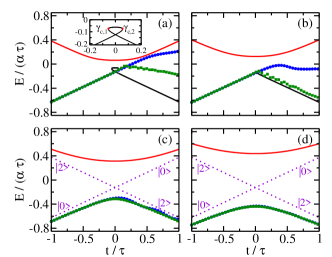
Figure 1: Scaled energy levels of $\hat{H}_{\text{TS}}$ for $C/(\alpha\tau)=0.268$ as a function of $t/\tau$ for (a) $C/\Omega=2.14$, (b) 1.07, (c) 0.428, and (d) 0.306. The black and red solid lines show the adiabatic energy levels [in panels (c) and (d), the black lines are covered by the symbols]. The blue circles and green squares show the dynamic energy levels for $\hbar/(\alpha\tau^{2})=7.68\times 10^{-2}$ and $\hbar/(\alpha\tau^{2})=7.68\times 10^{-3}$, respectively [in (d), the blue circles are covered by the green squares]. The tunneling probability is appreciable in (a) and (b) and essentially zero in (c) and (d). The inset in (a) shows an enlargement of the swallowtail; $\gamma_{\text{c},1}/(\alpha\tau)$ and $\gamma_{\text{c},2}/(\alpha\tau)$ correspond to the boundaries of the swallowtail. As a reference, the purple dotted lines in (c) and (d) show the adiabatic energy levels for $\Omega=0$; the energy levels are labeled by their eigenstates. The parameters used to make the solid lines and blue circles are the same as those used in Fig. 2.

This work realizes the non-linear Landau-Zener model experimentally by preparing a single-component BEC consisting of $N$ ⁸⁷Rb atoms of mass $m$ in the $|F,m_{F}\rangle=|1,-1\rangle$ hyperfine state in an optical dipole trap and by then adiabatically loading the BEC into a one-dimensional optical lattice $V_{\text{lat}}(z)$ latticeRMP ; peik1997 ; engels ; guan2020 . The optical lattice is created by two 1064 nm beams [with wave vectors $\vec{k}_{1}$ and $\vec{k}_{2}$, $|\vec{k}_{1}|=|\vec{k}_{2}|$, and angular frequencies $\omega_{1}(t)$ and $\omega_{2}(t)$] that cross at an angle of $\approx\pi/2$, $V_{\text{lat}}(z,t)=2\Omega\cos^{2}[k_{L}z-\phi(t)/2]$; $\Omega$ denotes the effective coupling strength, $k_{L}\approx|\vec{k}_{1}|/\sqrt{2}$, $\phi(t)=[\omega_{1}(t)-\omega_{2}(t)]t$ with $\phi(t)=0$ for $t<-\tau$, and $\delta_{L}(t)=\hbar\partial_{t}\phi(t)$. At $t=-\tau$, the optical dipole trap is turned off and the BEC, which has an average momentum close to zero, sits at the “bottom” of the first Brillouin zone; this corresponds to a good approximation to state $|0\rangle$. In our first set of experiments, $\delta_{L}(t)$ is—for $t>-\tau$—increased linearly from $0$ with ramp rate $\alpha=h\times 9$ kHz/ms. The time sequence is designed such that $\delta_{L}(0)$ is equal to $4$ $E_{L}$ and $\delta_{L}(\tau)$ is equal to $8$ $E_{L}$, i.e., such that the edge of the first Brillouin zone and the middle of the second Brillouin zone are reached when $t=0$ and $t=\tau$, respectively [here, $E_{L}=\hbar^{2}k_{L}^{2}/(2m)=h\times 1.08$ kHz]. In each repetition of the experiment, the ramp is stopped at various $t$ and the occupations of the components centered at vanishing momentum along the $z$-direction (state $|0\rangle$) and centered at momentum $2\hbar k_{L}$ (state $|2\rangle$) are measured after 16.5 ms time of flight, counted from the end of the ramp. During the time-of-flight expansion, the two momentum components separate fully in real space. The red circles in Fig. 2 show the experimentally determined population imbalance $\Delta b(t)$. It can be seen that the BEC occupies, for $t/\tau\gtrsim 0$, primarily state $|2\rangle$ when $\Omega$ is “large” and primarily state $|0\rangle$ when $\Omega$ is “small”.

The lattice system is described by the time-dependent GP equation with Hamiltonian $\hat{H}_{\text{GP}}$ latticeRMP ,

$$\hat{H}_{\text{GP}}=\hat{\vec{p}}^{2}/(2m)+V_{\text{lat}}(z,t)+g(N-1)|\Psi(\vec{r},t)|^{2}.$$ (5)

Here, $g$ is equal to $4\pi\hbar^{2}a_{s}/m$ and the mean-field orbital $\Psi(\vec{r},t)$ is normalized according to $\int|\Psi(\vec{r},t)|^{2}d\vec{r}=1$. For the $|1,-1\rangle$ state of ⁸⁷Rb, the $s$-wave scattering length $a_{s}$ is equal to $100.4$ $a_{\text{bohr}}$ scattering_length . Following the experimental protocol, the blue squares in Fig. 2 show our GP mean-field simulation results. The good agreement with the experimental data, including the reproduction of the oscillatory behavior of the population imbalance for $t\gtrsim 0$ and the small deviations of the population imbalance from $1$ for large $\Omega$ near $t\approx-\tau$, indicates that the mean-field framework captures the dynamics quite accurately.

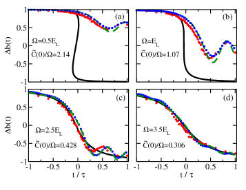
Figure 2: Experiment-theory comparison of population imbalance $\Delta b(t)$ in response to a linear ramp with $\alpha=h\times 9$ kHz/ms corresponding to $\hbar/(\alpha\tau^{2})=7.68\times 10^{-2}$] as a function of $t/\tau$ for various $\tilde{C}(0)/\Omega$. The experimental results (red circles) are for $N=3.1\times 10^{5}$, $\omega_{x,y,z}=2\pi\times(147,160,29.8)$ Hz, and $E_{L}=h\times 1.08$ kHz. The blue squares and green dashed lines are obtained from $\hat{H}_{\text{GP}}$ and $\hat{H}_{\text{TS,t}}$, respectively (analyzing the dynamic states). In both cases, the initial state is prepared in an axially symmetric trap with $\omega_{\rho}=(\omega_{x}+\omega_{y})/2$. The mean-field energy $\tilde{C}(t)$ is equal to $1.27$ $E_{L}$ and $1.07$ $E_{L}$ for $t=-\tau$ and $t=0$, respectively. For comparison, the black solid lines show $\Delta b(t)$ for the lower adiabatic eigenstate of $\hat{H}_{\text{TS,t}}$.

To bring out the two-state nature of the lattice system, we write niu1 ; zobay ; guan2020 $\Psi(\vec{r},t)=\psi_{0}(\vec{r},t)+\psi_{2}(\vec{r},t)\exp(2\imath k_{L}z)$, i.e., we assume that the populations of the $n\hbar k_{L}$ momentum components with $n=-2,\pm 4,\pm 6,\cdots$ are small guan2020 . Inserting the ansatz into the non-linear time-dependent GP equation, the Supplemental Material SM develops a semi-analytical framework that yields a spatially-independent two-state Hamiltonian $\hat{H}_{\text{TS,t}}$. The Hamiltonian $\hat{H}_{\text{TS,t}}$ is identical to $\hat{H}_{\text{TS}}$ provided the mapping $\gamma(t)\rightarrow-4E_{L}+\delta_{L}(t)$ and $C\rightarrow\tilde{C}(t)$ is applied. The time-dependent mean-field energy $\tilde{C}(t)$, $\tilde{C}(t)=g(N-1)\bar{n}(t)$, accounts for the fact that the BEC expands during the ramp, thereby resulting in a decrease of the mean density $\bar{n}(t)$ with increasing $\gamma(t)$. Since we are interested in non-linear effects, the decrease of the mean-field energy during the ramp places a constraint on $\alpha$ for a given $\tilde{C}(-\tau)/\Omega$. Figure S1 in the Supplemental Material SM shows the adiabatic and dynamic energy levels of the Hamiltonian $\hat{H}_{\text{TS,t}}$ for the experimental parameters used in Fig. 2. Comparison with Fig. 1 shows that the adiabatic and dynamic energy levels supported by $\hat{H}_{\text{TS}}$ and $\hat{H}_{\text{TS,t}}$ agree quite well.

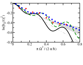
Figure 3: Experiment-theory comparison of tunneling probability $|b_{0}(t)|^{2}$ at $t=\tau$ in response to linear ramps with varying $\alpha$ for $\tilde{C}(-\tau)/\Omega=2.75$ as a function of $\pi\Omega^{2}/(2\hbar\alpha)$. The experimental results (red circles; the error bars show the standard deviation from three independent runs) are for $N=2.3\times 10^{5}$, $\omega_{x,y,z}=2\pi\times(193,218,29.8)$ Hz, $E_{L}=h\times 1.08$ kHz, and $\Omega=0.52$ $E_{L}$. The blue squares and green dashed lines are obtained for $\hat{H}_{\text{GP}}$ and $\hat{H}_{\text{TS,t}}$, respectively [analyzing the dynamic states; the initial state is prepared in an axially symmetric trap with $\omega_{\rho}=(\omega_{x}+\omega_{y})/2$]. Both data sets follow the non-exponential trend of the grey-shaded region, which shows Eq. (S11) for $C/\Omega$ values ranging from $\tilde{C}(-\tau)/\Omega$ to $\tilde{C}(0)/\Omega$ SM . The black solid line, which oscillates around the linear Landau-Zener formula [grey dash-dotted line; Eq. (1)], shows the tunneling probability for $\hat{H}_{\text{TS}}$ with $C=0$. The experimental data are better described by the non-exponential grey-shaded family of curves than by the linear Landau-Zener formula.

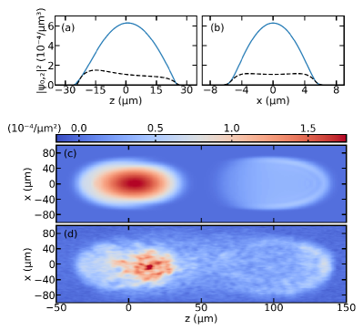
Figure 4: Theoretical GP and experimental densities for the ramp ending at $t=-\tau+0.6$ ms [$t/\tau=0.25$ in Fig. 2(b)]. (a) and (b) show density cuts before time-of-flight expansion for $\rho=0$ and $y=z=0$, respectively. The blue solid and black dashed lines are for states $\psi_{0}(\vec{r},t)$ and $\psi_{2}(\vec{r},t)$, respectively. (c) and (d) show, respectively, theoretical and experimental integrated densities $n(x,z,t)$, $n(x,z,t)=\int_{-\infty}^{\infty}|\Psi(\vec{r},t)|^{2}dy$, after $16.5$ ms time-of-flight expansion.

Black solid and green dashed lines in Fig. 2 show the decomposition of the states corresponding to, respectively, the lower adiabatic and lower dynamic energy levels supported by $\hat{H}_{\text{TS,t}}$. It can be seen that the green dashed lines agree reasonably well with the experimental and GP results; this confirms the applicability of the non-linear two-state Hamiltonian to the lattice system. Moreover, it can be seen that the decomposition of the states corresponding to the adiabatic and dynamic energy levels agree for the largest $\Omega$ value considered [Fig. 2(d)] but differ for the other $\Omega$ values. This shows that the system dynamics are, for fixed ramp rate $\alpha$, adiabatic for the largest $\Omega$ considered in Fig. 2 but not for the other $\Omega$ values. In Fig. 2(c), the experimental data and populations extracted from the dynamic energy level oscillate around the populations extracted from the adiabatic energy level Han2015 . In Figs. 2(a) and 2(b), the experimental data and populations extracted from the dynamic energy level oscillate as well for $t\gtrsim 0$; however, the oscillations are not centered around the populations extracted from the adiabatic energy level but instead lie notably above. Our theory analysis shows that the enhanced tunneling probability (enhanced probability to remain in state $|0\rangle$) is due to self-trapping, a phenomenon inherently linked to the presence of swallowtails niu5 .

While the inhibition of transitions to state $|2\rangle$ due to non-linear interactions has been previously observed in an optical lattice system similar to ours gadway as well as in coupled double-well type set-ups bloch ; albiez ; steinhauer and annular rings campbell , we now show—for the first time in this context—evidence for non-exponential tunneling. Red circles in Fig. 3 show the experimentally measured population of state $|0\rangle$ for $t=\tau$ and $\tilde{C}(-\tau)/\Omega=2.75$; this ratio is a bit larger than that used in Fig. 2(a). It can be seen that the experimental data, which are obtained by varying the ramp rate $\alpha$ (and correspondingly $\tau$ such that $\alpha\tau$ is equal to $4$ $E_{L}$), display an overall decrease with increasing $\pi\Omega^{2}/(2\hbar\alpha)$. The experimental data are quite well reproduced by our GP simulations (blue squares). The decomposition of the state corresponding to the lower dynamic energy level of $\hat{H}_{\text{TS,t}}$ (green dashed line) yields notably larger oscillations but displays the same overall trend. In the $\tau\rightarrow\infty$ limit, the tunneling probability of the non-linear two-state model $\hat{H}_{\text{TS}}$ varies non-exponentially with $\pi\Omega^{2}/(2\hbar\alpha)$ SM . The grey-shaded region shows the results for $C/\Omega$ values between $\tilde{C}(-\tau)/\Omega=2.75$ (upper bound) and $\tilde{C}(0)/\Omega$ (lower bound; this value varies with the ramp rate), respectively. The experimental and GP data exhibit small oscillations around the grey region, which can be viewed as a “smoothed” version of the green-dashed line. For comparison, the black solid line shows the results for the non-interacting two-state model. Due to the finite time window, the black solid line oscillates around the “linear Landau-Zener” formula [Eq. (1), grey dash-dotted line]. A key observation of our work is that the experimental data are much better described by the non-exponential grey-shaded region than the linear Landau-Zener formula. Figure 3 provides the first experimental verification of non-exponential tunneling dynamics, driven by swallowtails.

Figure 3 also shows that the oscillation amplitude of $\ln[|b_{0}(t)|^{2}]$ is smaller for the experimental and GP data than for the finite-$\tau$ two-state model data. We attribute this to intricate internal dynamics, which are not accounted for by the two-state models $\hat{H}_{\text{TS}}$ and $\hat{H}_{\text{TS,t}}$. To illustrate the internal dynamics, Figs. 4(a) and 4(b) show GP densities for the ramp stopped at $t/\tau=0.25$ in Fig. 2(b) (no time-of-flight expansion). The density cuts for the finite momentum component deviate from a simple Thomas-Fermi profile; in particular, the density along $z$ for $\rho=0$ is deformed, exhibiting a maximum at negative $z$, and the density along $x$ for $y=z=0$ exhibits a double peak structure [black dashed lines in Figs. 4(a) and 4(b), respectively]. These density deformations develop during the ramp and are attributed to the interplay between the on-site and off-site mean-field interactions (see Supplemental Material SM ).

Figures 4(c) and 4(d) show GP and experimentally measured integrated densities after $16.5$ ms time-of-flight expansion for the same ramp as considered in Figs. 4(a) and 4(b). The overall agreement between theory and experiment is excellent. The zero-momentum component (centered around $z=0$) has its maximum at positive $z$ while the finite-momentum component (centered around $z\approx 100$ $\mu$m) displays an enhanced density that is located on a half-ring on the right edge of the cloud. During the time-of-flight expansion, the finite-momentum component moves relative to the zero-momentum component: To reduce mean-field interactions, the finite-momentum component accumulates density first at the left edge of the cloud and later at the right edge of the cloud. The theory data indicate that the relative motion of the two clouds generates low energy excitations [wave-like density pattern in Fig. 4(c)]; although not clearly resolved, faint indications of these patterns are visible in the experimental images.

Quantum tunneling is ubiquitous in physics: it plays a central role in high-energy, nuclear, atomic, and condensed matter physics as well as in chemistry, biology, and engineering. Modern physics courses introduce students to quantum tunneling and exponentially decaying tunneling probabilities. The full quantum treatment, however, shows that quantum tunneling is much richer, necessitating deviations from the exponential decay in both the short- and long-time regimes fonda ; greenland . Indeed, deviations from exponential decay were observed in the short-time regime in a pioneering experiment with cold atoms loaded into an accelerated optical lattice raizen . The deviations from purely exponential tunneling probabilities observed in this work are fundamentally different; they have their origin in the non-linearity of the interactions. Non-linearities also play a fundamental role in the tunneling of a BEC out of an external trap into the continuum potnis2017 ; zhao2017 . In that case, however, the non-linear Landau-Zener model cannot be applied. Our work is also fundamentally different from the non-exponential decay analyzed theoretically in Floquet-Bloch bands weld , where the emphasis lies on short-time deviations and oscillations due to a finite energy window and not due to non-linear mean-field interactions.

Acknowledgement: Support by the National Science Foundation through grant numbers PHY-1806259 (QG and DB) and PHY-1607495/PHY-1912540 (MKHO, TMB, SM, and PE) are gratefully acknowledged. This work used the OU Supercomputing Center for Education and Research (OSCER) at the University of Oklahoma (OU).

.1 Selected properties of $\hat{H}_{\text{TS}}$

This section discusses selected properties of the two-state Hamiltonian $\hat{H}_{\text{TS}}$. We first discuss why the validity of the linear Landau-Zener formula [Eq. (1) of the main text] requires $\Omega/(\alpha\tau)\ll 1$. To see this, we consider the adiabatic eigenenergies $\lambda_{\pm}(t)$ of $\hat{H}_{\text{TS}}$,

$$\lambda_{\pm}(t)=\pm\frac{1}{2}\sqrt{\Omega^{2}+\left[\gamma(t)-C\Delta b(t)\right]^{2}},$$ (S1)

where $\Delta b(t)$ implicitly depends on $\Omega$, $\gamma(t)$, and $C$. For $C=0$, the adiabatic eigenenergies can be rewritten as

$$\frac{\lambda_{\pm}(t)}{\alpha\tau}=\pm\frac{1}{2}\sqrt{\left(\frac{t}{\tau}\right)^{2}+\left(\frac{\Omega}{\alpha\tau}\right)^{2}}.$$ (S2)

The derivation of the linear Landau-Zener formula assumes that the initial state $\vec{b}(-\tau)=(1,0)^{T}$ is, to a very good approximation, equal to the lowest eigenstate of $\hat{H}_{\text{TS}}$ for $C=\Omega=0$ and $t=-\tau$; this eigenstate has an energy of $-\alpha\tau/2$. Looking at Eq. (S2), the condition on the initial state can be expressed as $\lambda_{-}(-\tau)$ being approximately equal to $-\alpha\tau/2$ for $t=-\tau$. This condition translates to $[\Omega/(\alpha\tau)]^{2}\ll 1$.

Since $\alpha\tau$ emerges as the reference energy scale when analyzing the adiabatic eigenenergies, we refer to it as “static” energy scale $U_{s}$. The natural time scale associated with $U_{s}$ is given by $T_{s}=\hbar/U_{s}$. To obtain the dimensionless ramp rate $\tilde{\alpha}$, we need to divide $\alpha$ by $U_{s}/T_{s}$. This yields $\tilde{\alpha}=\hbar/(\alpha\tau^{2})$. Somewhat counterintuitively, the dimensionless ramp rate $\tilde{\alpha}$ is inversely proportional to $\alpha$. When $\alpha\tau$ is fixed (this is the case in the experiments discussed in Figs. 2-4 of the main text), it is most natural to think about the ramp in terms of the dimensionless ramp rate $\tilde{\alpha}$. In Fig. 3 of the main text, e.g., the ramp rate $\alpha$ changes from $37.2$ $E_{L}$/ms (left most red circle) to $4.52$ $E_{L}$/ms (right most red circle); these values correspond to $\tilde{\alpha}=0.343$ and $0.0416$, respectively.

Alternatively, we may choose $\tau$ as our natural time unit. In this alternative set of units, the energy unit is given by $U_{d}$, $U_{d}=\hbar/\tau$. We refer to $U_{d}$ as “dynamic” energy scale, since it emerges by defining the time unit through $\tau$. In these alternative units, the dimensionless ramp rate is given by $\alpha\tau^{2}/\hbar$ (i.e., by $\tilde{\alpha}^{-1}$). The dimensionless ramp rate $\tilde{\alpha}$ is equal to the scale ratio $U_{d}/U_{s}$. The $\tilde{\alpha}\ll 1$ regime corresponds to $U_{s}\gg U_{d}$; this is the adiabatic regime.

.2 Derivation of two-state Hamiltonian

Starting with the time-dependent GP equation, this section derives the spatially independent non-linear two-state Hamiltonian $\hat{H}_{\text{TS,t}}$. The states $\psi_{0}(\vec{r},t)$ and $\psi_{2}(\vec{r},t)$, which are introduced in the main text, are assumed to be localized in the vicinity of the momenta $\hbar k_{z}=0$ and $\hbar k_{z}=2\hbar k_{L}$, respectively, and normalized such that $\sum_{j=0,2}\int|\psi_{j}(\vec{r},t)|^{2}d\vec{r}=1$. As in Ref. Sguan2020 , we assume that the widths of the momentum distributions associated with the states ${\psi}_{0}({\vec{r}},t)$ and ${\psi}_{2}({\vec{r}},t)$ are narrow compared to $2\hbar k_{L}$. For the initial states used in Figs. 2 and 3 of the main text, the full-width-half-maxima of the momentum distributions along the $z$-direction are $\hbar\times 0.149$ $\mu$m^-1 and $\hbar\times 0.141$ $\mu$m^-1, respectively; for comparison, $2\hbar k_{L}$ is equal to $\hbar\times 8.62$ $\mu$m^-1 (i.e., roughly $60$ times larger). As a result, we find the following approximate spatially- and time-dependent mean-field Hamiltonian Sguan2020 :

$$\hat{{{H}}}=I_{2}\hat{H}_{0}+\hat{H}_{1}+\frac{1}{2}\begin{pmatrix}\gamma(t)-g(N-1)(|{\psi}_{0}({\vec{r}},t)|^{2}-|{\psi}_{2}({\vec{r}},t)|^{2})&\Omega\\ \Omega&-\gamma(t)+g(N-1)(|{\psi}_{0}({\vec{r}},t)|^{2}-|{\psi}_{2}({\vec{r}},t)|^{2})\\ \end{pmatrix},$$ (S3)

where

$$I_{2}=\begin{pmatrix}1&0\\ 0&1\end{pmatrix},$$ (S4)

$$\hat{H}_{0}=\frac{\hat{\vec{p}}^{2}}{2m}+\frac{3g(N-1)}{2}\left(|{\psi}_{0}({\vec{r}},t)|^{2}+|{\psi}_{2}({\vec{r}},t)|^{2}\right)+\frac{4E_{L}-\delta_{L}(t)}{2},$$ (S5)

$$\hat{H}_{1}=\frac{2\hbar k_{L}}{m}\begin{pmatrix}0&0\\ 0&\hat{p}_{z}\end{pmatrix},$$ (S6)

and

$$\gamma(t)=-4E_{L}+\delta_{L}(t).$$ (S7)

We now make the ansatz that the spatial orbitals $\psi_{j}(\vec{r},t)$ for the $j=0$ and $j=2$ components are identical and that the occupations of the two components are parametrized by $|b_{j}(t)|^{2}$,

$$\psi_{j}(\vec{r},t)=b_{j}(t)\varphi_{\text{TF}}(\vec{r},t),$$ (S8)

where the normalizations read $\int|\varphi_{\text{TF}}(\vec{r},t)|^{2}d\vec{r}=1$ and $|b_{0}(t)|^{2}+|b_{2}(t)|^{2}=1$. At $t=-\tau$, the spatial orbital $\varphi_{\text{TF}}(\vec{r},t)$ is equal to the Thomas-Fermi orbital for a harmonically trapped $N$-particle BEC. We then assume that the component densities maintain their Thomas-Fermi shape during the ramp. Specifically, we assume that $\varphi_{\text{TF}}(\vec{r},t)$ expands during the ramp in the same manner as a single-component $N$-atom BEC. This implies that the time evolution of $\varphi_{\text{TF}}(\vec{r},t)$ is governed by the self-similar solutions derived by Castin and Dum SCastin . The adapted formulation neglects the relative motion along the $z$-direction of the two components with respect to each other. Moreover, the formulation does not allow for deviations from the Thomas-Fermi density (structure formation). Correspondingly, the description should work best for fast ramps and deteriorate for slower ramps.

Integrating over the spatial degrees of freedom, we find the Hamiltonian $\hat{H}_{\text{TS,t}}$,

$$\hat{H}_{\text{TS,t}}=$$

$$\frac{1}{2}\left(\begin{array}[]{cc}\gamma(t)-\tilde{C}(t)\Delta b(t)&\Omega\\ \Omega&-\gamma(t)+\tilde{C}(t)\Delta b(t)\end{array}\right),$$ (S11)

where

$$\tilde{C}(t)=g(N-1)\int|\varphi_{\text{TF}}(\vec{r},t)|^{4}d\vec{r}.$$ (S12)

Here $\Delta b(t)$ is, as in the main text, equal to $|b_{0}(t)|^{2}-|b_{2}(t)|^{2}$. In going from Eq. (S3) to Eq. (.2), we assumed that $\int\varphi^{*}_{\text{TF}}(\vec{r},t)\hat{p}_{z}\varphi_{\text{TF}}(\vec{r},t)d\vec{r}$ vanishes, i.e., that the spatial average of $\hat{H}_{1}$ vanishes. Neglecting the effect of the $\hat{p}_{z}$ term is consistent with our earlier assumption that the components do not move relative to each other during the ramp. In addition, we dropped the time-dependent scalar $\int\varphi^{*}_{\text{TF}}(\vec{r},t)\hat{H}_{0}\varphi_{\text{TF}}(\vec{r},t)d\vec{r}$. This time-dependent scalar can be rotated away by introducing an overall time-dependent phase, i.e., this part of the Hamiltonian does not impact the physics. We reiterate that the Hamiltonian $\hat{H}_{\text{TS,t}}$ should work best for fast ramps.

The reduction of the GP description of the lattice system to the two-state Hamiltonian $\hat{H}_{\text{TS,t}}$ establishes, as discussed in the main text, a connection between the recoil energy $E_{L}$, the beginning and end time $\tau$ of the ramp (assuming a full ramp), and the ramp rate $\alpha$: $\alpha\tau=4E_{L}$. Thus, for a fixed lattice geometry, a smaller ramp rate $\alpha$ is necessarily accompanied by a larger $\tau$. Since a larger $\tau$ implies a larger decrease of the mean-field energy during the ramp, one might ask if there are alternative approaches to adjusting the ramp rate while maintaining a sufficiently large and approximately constant mean-field energy during the ramp. We now discuss two such approaches. (i) We performed a sequence of experiments in which the external harmonic trapping potential was kept on during the ramp. In this case, the BEC does not expand during the ramp and the mean-field energy is maintained. We found that this alternative approach leads to a fair bit of heating during the ramp, in addition to competing dynamics that are influenced by the harmonic confinement. We concluded that this approach does create more challenges than it solves. (ii) One could repeat the experiments discussed in our work for lattices with a different recoil energy. For example, using a lattice with a larger recoil energy $E_{L}$ would, for fixed $\tau$, translate to a larger $\alpha$ and thus to a smaller dimensionless ramp rate $\tilde{\alpha}$. The experimental implementation of this is beyond the scope of the present work.

As mentioned in the main text, our GP simulations prepare the initial state $\Psi(\vec{r},-\tau)$ assuming an axially symmetric trap. Even though the dynamics after turning the external harmonic confinement off, i.e., during the ramp and subsequent time-of-flight expansion, could—in principle—introduce excitations along the azimuthal angle, this degree of freedom is not treated explicitly in our GP numerics. The restriction to an axially symmetric mean-field orbital $\Psi(\vec{r},t)$ appears to provide a realistic description of the dynamics.

.3 Considerations related to Fig. 2 of the main text

Figure 2 of the main text analyzes the population imbalance $\Delta b(t)$ for four different $\tilde{C}(0)/\Omega$ values that range from the mean-field-energy-dominated to the lattice-coupling-strength-dominated regime. To complement the discussion, Fig. S1 shows the adiabatic and dynamic energy levels of the two-state Hamiltonian $\hat{H}_{\text{TS,t}}$ for the same parameters as considered in Fig. 2 of the main text. It can be seen that the adiabatic and dynamic energy levels supported by $\hat{H}_{\text{TS,t}}$ agree quite well with those shown in Fig. 1 of the main text. Recall, Fig. 1 of the main text uses a constant $C$ value, namely $C=\tilde{C}(0)$, but otherwise the same parameters as Fig. S1. As a consequence, the energy gap at $t=0$ in Fig. S1 is equal to that in Fig. 1 of the main text. The time dependence of the mean-field energy introduces a slight asymmetry into the adiabatic energy levels, i.e., $t=0$ defines no longer a symmetry point. Specifically, compared to Fig. 1 of the main text, the adiabatic energy levels supported by $\hat{H}_{\text{TS,t}}$ are shifted upward for $t>0$; the upward shift increases with increasing time due to the decrease of $\tilde{C}(t)$.

Generalizing the derivation presented in Sec. .2 to include the $\hbar k_{z}=4\hbar k_{L}$ component, we derived a three-state model. The three-state model yields similar results as the two-state model for the parameter regimes considered in this work. This shows that the impact of the higher momentum components is negligible and that the two-state model captures the key aspects of the lattice system in the parameter regime considered in this work.

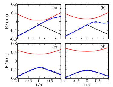
Figure S1: Adiabatic and dynamic energy levels as a function of $t/\tau$ for (a) $\tilde{C}(0)/\Omega=2.14$, (b) $1.07$, (c) $0.428$, and (d) $0.306$; the initial states and parameter combinations considered in this figure are the same as in Fig. 2 of the main text. The black and red solid lines show the lower and upper adiabatic energy levels of $\hat{H}_{\text{TS,t}}$. The blue circles show the lower dynamic energy level of $\hat{H}_{\text{TS,t}}$ for $\hbar/(\alpha\tau^{2})=7.68\times 10^{-2}$.

.4 Tunneling probability for the two-state Hamiltonian $\hat{H}_{\text{TS}}$

The tunneling probabilities for the two-state Hamiltonian $\hat{H}_{\text{TS}}$ were derived in Ref. Sniu2 . For $C/\Omega\geq 1$, the tunneling probability $r$ is determined by the equation Sniu2

$$\frac{1}{1-r}=\frac{1}{1-\exp\left(-\frac{\pi\Omega^{2}}{2\hbar\alpha}\right)}+\frac{\sqrt{2}}{\pi}\frac{C}{\Omega}\sqrt{1-r}.$$ (S13)

For $C/\Omega<1$, one obtains in the adiabatic limit the modified exponential Landau-Zener tunneling formula Sniu2

$$r=\exp\left(-q\frac{\pi\Omega^{2}}{2\hbar\alpha}\right),$$ (S14)

where the scaling factor $q$ is given by

$$q=\frac{4}{\pi}\times$$

$$\int_{0}^{\sqrt{\left(\frac{\Omega}{C}\right)^{2/3}-1}}(1+x^{2})^{1/4}\left[\frac{1}{(1+x^{2})^{{3/2}}}-\frac{C}{\Omega}\right]^{3/2}dx.$$ (S15)

The grey-shaded region in Fig. 3 of the main text shows Eq. (S13) with $C$ values ranging from $C=\tilde{C}(-\tau)$ to $C=\tilde{C}(0)$. While one might naively think that it would be more appropriate to use $C=\tilde{C}(0)$, i.e., the value of the mean-field energy at the mid-point of the ramp, it should be kept in mind that the tunneling probability is an integrated quantity whose value accumulates during the ramp. Moreover, in the non-linear Landau-Zener model, the tunneling probability at each time depends on the populations and thus indirectly on the amount of tunneling that occurred during the earlier part of the ramp. For these reasons, there exists no clear argument for how to choose the value of $C$ when using the non-linear two-state model with time-independent $C$ to describe the results obtained using our optical lattice implementation, which is characterized by a time-dependent mean-field energy.

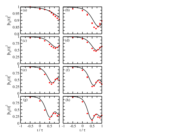
Figure S2: Extended experimental data sets corresponding to Fig. 3 of the main text; panels (a)-(h) correspond to the eight (from left to right) experimental data points shown in Fig. 3 of the main text. Each red circle is the average of three independent experimental runs; the error bars, which are hardly visible, show the standard deviation. The uncertainties (not shown) of the populations extracted from the GP simulations (solid lines) due to the use of finite spatial grid spacings and a finite time step are estimated to be smaller than the experimental error bars. Note the different ranges of the vertical axis in (a)-(b) and (c)-(h).

.5 Extended data sets in the mean-field-dominated regime

Figure S2 shows extended experimental data sets associated with Fig. 3 of the main text. The red circles in Figs. S2(a)-S2(h) show the experimentally measured populations $|b_{0}(t)|^{2}$ of the zero-momentum component as a function of time for different ramp rates $\alpha$. It can be seen that the agreement between the GP equation based results (black lines) and the experimental data (red circles) is quite good. The data in Fig. S2 show a delayed onset of population transfer consistent with self-trapping. The population for the largest time, i.e., for $t=\tau$, is used to make Fig. 3 of the main text.

.6 Tunneling probability in the lattice-coupling-strength-dominated regime

Figure 3 of the main text analyzes the tunneling probabilities in the mean-field-dominated regime but not in the lattice-coupling-strength-dominated regime. To elucidate why the analysis of the tunneling probabilities in the lattice-coupling-strength-dominated regime considered in Figs. 2(c) [$\Omega/(\alpha\tau)=0.625$] and 2(d) [$\Omega/(\alpha\tau)=0.875$] of the main text is challenging, Fig. S3 plots the logarithm of $|b_{0}(\tau)|^{2}$ as a function of $\pi\Omega^{2}/(2\hbar\alpha)$. The red circles show the experimental data points corresponding to the linear ramp considered in Fig. 2 of the main text. The blue squares show results from the GP simulations for different ramp rates $\alpha$ but otherwise identical parameters. For comparison, the black solid lines show the tunneling probability obtained using the two-state Hamiltonian $\hat{H}_{\text{TS,t}}$. It can be seen that the tunneling probabilities in Figs. S3(c) and S3(d) oscillate wildly; in particular, the probabilities do not seem to be oscillating around a monotonically decaying “background curve”. The “wild oscillations” are attributed to the finite time window. The oscillations become more regular when $\tau$ is, for fixed ramping rate $\alpha$, increased. This is illustrated by the black solid lines in the insets of Figs. S3(c) and S3(d), which show the results for Hamiltonian $\hat{H}_{\text{TS,t}}$ using $\tau=12$ $E_{L}/\alpha$ (i.e., a three times larger $\tau$) but otherwise identical parameters. The oscillation amplitude decreases with increasing $\tau$ while the oscillation frequency increases. The insets in Figs. S3(c) and S3(d) show that $\ln(|b_{0}(\tau)|^{2})$ oscillates around a straight line with a slope close to $-1$. This implies that the tunneling probability is, on average and provided $\tau$ is sufficiently large, reasonably well described by the standard linear Landau-Zener formula in the strong lattice-coupling-strength regime.

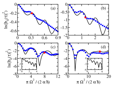
Figure S3: Logarithm of $|b_{0}(\tau)|^{2}$ as a function of $\pi\Omega^{2}/(2\hbar\alpha)$ for (a) $\tilde{C}(0)/\Omega=2.14$, (b) $1.07$, (c) $0.428$, and (d) $0.306$; the initial states and parameters considered in this figure are, except for $\alpha$, the same as in Fig. 2 of the main text. The values of $\Omega/(\alpha\tau)$ for panels (a)-(d) are 0.125, 0.25, 0.625, and 0.875, respectively. The red circles, which are extracted from Fig. 2 of the main text, show experimental results for $\alpha=h\times 9$ kHz/ms (corresponding to $\alpha\tau=4$ $E_{L}$). The blue squares show GP results for varying $\alpha$. For comparison, the black solid lines show results extracted from the lower dynamic energy level supported by $\hat{H}_{\text{TS,t}}$. The insets of (c) and (d) show results extracted from the lower dynamic energy level of $\hat{H}_{\text{TS,t}}$ with $\alpha\tau=12$ $E_{L}$. Note that the ranges of the axis in the insets are different than those in the main figures.

.7 Integrated densities at the end of the ramp

The analysis in this section is based on the GP orbital $\Psi(\vec{r},t)$. Figures 4(a) and 4(b) of the main text show density cuts at the end of the ramp, i.e., prior to the time-of-flight expansion (recall that the ramp sequence is not part of the time-of-flight expansion in our convention), while Figs. 4(c) and 4(d) of the main text show integrated densities after the time-of-flight expansion. Since the ramp time is relatively short, the two momentum components $\psi_{j}(\vec{r},t)$ ($j=0$ and $2$) overlap to a good approximation in real space at the end of the ramp. To “isolate” the two components $\psi_{j}(\vec{r},t)$, we transform $\Psi(\vec{r},t)$ to momentum space,

$$\Phi(\vec{k},t)=\frac{1}{(2\pi)^{3/2}}\int\Psi(\vec{r},t)\exp\left(-\imath\vec{k}\cdot\vec{r}\right)d\vec{r}.$$ (S16)

Since $\Phi(\vec{k},t)$ has two distinct peaks centered around $k_{z}=0$ and $k_{z}=2k_{L}$, we define the Fourier-transform of $\psi_{0}(\vec{r},t)$ as the part of $\Phi(\vec{k},t)$ with $k_{z}<k_{L}$ and the Fourier-transform of $\psi_{2}(\vec{r},t)$ as the part of $\Phi(\vec{k},t)$ with $k_{z}>k_{L}$,

$$\psi_{0}(\vec{r},t)=\frac{1}{(2\pi)^{3/2}}\int\Phi(\vec{k},t)\Theta(k_{L}-k_{z})d\vec{k}$$ (S17)

and

$$\psi_{2}(\vec{r},t)=\frac{1}{(2\pi)^{3/2}}\int\Phi(\vec{k},t)\Theta(k_{z}-k_{L})d\vec{k},$$ (S18)

where the step function $\Theta(x)$ is equal to $1$ for $x>0$ and equal to $0$ for $x<0$.

The cuts shown in Figs. 4(a) and 4(b) of the main text are calculated using Eqs. (S16)-(S18). To complement the density cuts discussed in the main text, Figs. S4(a) and S4(b) show the corresponding integrated densities $n_{j}(x,z,t)$ for $j=0$ and $j=2$, respectively, for $t=-\tau+0.6$ ms, i.e., prior to the time-of-flight expansion (same time as the density cuts). The $n_{j}(x,z,t)$ are defined by integrating over the $y$-coordinate, $n_{j}(x,z,t)=\int_{-\infty}^{\infty}|\psi_{j}(\vec{r},t)|^{2}dy$. The integrated $j=0$ component density is approximately elliptical with a peak located at $\vec{r}=0$. The maximum of the integrated $j=2$ component density, in contrast, is located at negative $z$. The asymmetry of the $j=2$ component density develops during the $0.6$ ms short linear ramp, which allows for a tiny movement of the two momentum components relative to each other. The fact that the internal structures of the $j=0$ and $j=2$ densities differ can be understood by combining the mean-field terms in Eqs. (S3) and (S5). This yields

$$(N-1)\begin{pmatrix}g|\psi_{0}(\vec{r},t)|^{2}+2g|\psi_{2}(\vec{r},t)|^{2}&0\\ 0&2g|\psi_{0}(\vec{r},t)|^{2}+g|\psi_{2}(\vec{r},t)|^{2}\end{pmatrix};$$ (S19)

the “factor of 2” is due to exchange interactions Sguan2020 . For $t$ not much larger than $-\tau$, $|\psi_{2}(\vec{r},t)|^{2}$ is close to zero. This implies that the dynamics of the $j=0$ component is dominated by self-interactions while that of the $j=2$ component is governed by (factor of 2 larger) exchange interactions. As a consequence, the $j=2$ component feels an enhanced repulsive mean-field potential that is created by the $j=0$ component, thereby explaining the density deformation visible in Fig. S4.

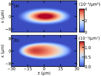
Figure S4: Integrated GP densities $n_{j}(x,z,t)$, $n_{j}(x,z,t)=\int_{-\infty}^{\infty}|\psi_{j}(\vec{r},t)|^{2}dy$, for $t=-\tau+0.6$ ms, i.e., before the time-of-flight expansion, for (a) $j=0$ and (b) $j=2$. The parameters are the same as those considered in Fig. 4 of the main text.

During the time-of-flight expansion, the integrated densities of the two components change significantly. This is highlighted by comparing Fig. S4(a) and the left parts of Figs. 4(c) and 4(d) of the main text as well as Fig. S4(b) and the right parts of Figs. 4(c) and 4(d) of the main text. The dynamics during the time-of-flight expansion are influenced by collisions between atoms within each of the two components as well as by collisions between particles with different $z$-momenta. During the expansion, the $j=2$ component “moves through” the $j=0$ component. The dynamics are governed by the fact that there exists a tendency to reduce the overlap between the $j=0$ and $j=2$ components. As discussed above, the peak of the $j=2$ density is displaced a bit to negative $z$ at the beginning of the time-of-flight expansion. This imbalance is enhanced during the initial stage of the expansion: with increasing expansion time, the density of the $j=2$ component on the negative $z$ side increases. Eventually, the density becomes too large, creating an energy penalty as opposed to an energy reduction. As a result, the $j=2$ density redistributes such that the highest density accumulates at the most positive $z$. The above discussion shows that the interplay of the two different momentum space components during the ramp and the time-of-flight expansion is due to intricate momentum space interactions.

References

- (1) L. Landau, Zur Theorie der Energieübertragung. II., Physikalische Zeitschrift der Sowjetunion 2, 46 (1932).
- (2) C. Zener, Non-Adiabatic Crossing of Energy Levels, Proc. R. Soc. Lond. A 137, 696 (1932).
- (3) B. Wu and Q. Niu, Nonlinear Landau-Zener tunneling, Phys. Rev. A 61, 023402 (2000).
- (4) O. Zobay and B. M. Garraway, Time-dependent tunneling of Bose-Einstein condensates, Phys. Rev. A 61, 033603 (2000).
- (5) J. Liu, L. Fu, B.-Y. Ou, S.-G. Chen, D.-I. Choi, B. Wu, and Q. Niu, Theory of non-linear Landau-Zener tunneling, Phys. Rev. A 66, 023404 (2002).
- (6) B. Wu, R. B. Diener, and Q. Niu, Bloch waves and bloch bands of Bose-Einstein condensates in optical lattices, Phys. Rev. A 65, 025601 (2002).
- (7) D. Diakonov, L. M. Jensen, C. J. Pethick, and H. Smith, Loop structure of the lowest Bloch band for a Bose-Einstein condensate, Phys. Rev. A 66, 013604 (2002).
- (8) E. J. Mueller, Superfluidity and mean-field energy loops: Hysteretic behavior in Bose-Einstein condensates, Phys. Rev. A 66, 063603 (2002).
- (9) M. Machholm, C. J. Pethick, and H. Smith, Band structure, elementary excitations, and stability of a Bose-Einstein condensate in a periodic potential, Phys. Rev. A 67, 053613 (2003).
- (10) O. Morsch, J. H. Müller, M. Cristiani, D. Ciampini, and E. Arimondo, Bloch Oscillations and Mean-Field Effects of Bose-Einstein Condensates in 1D Optical Lattices, Phys. Rev. Lett. 87, 140402 (2001).
- (11) M. Cristiani, O. Morsch, J. H. Müller, D. Ciampini, and E. Arimondo, Experimental properties of Bose-Einstein condensates in one-dimensional optical lattices: Bloch oscillations, Landau-Zener tunneling, and mean-field effects, Phys. Rev. A 65, 063612 (2002).
- (12) M. Jona-Lasinio, O. Morsch, M. Cristiani, N. Malossi, J. H. Müller, E. Courtade, M. Anderlini, and E. Arimondo, Asymmetric Landau-Zener Tunneling in a Periodic Potential, Phys. Rev. Lett. 91, 230406 (2003).
- (13) D. Witthaut, E. M. Graefe, and H. J. Korsch, Towards a generalized Landau-Zener formula for an interacting Bose-Einstein condensate in a two-level system, Phys. Rev. A 73, 063609 (2006).
- (14) A. Zenesini, C. Sias, H. Lignier, Y. Singh, D. Ciampini, O. Morsch, R. Mannella, E. Arimondo, A. Tomadin, and S. Wimberger, Resonant tunneling of Bose- Einstein condensates in optical lattices, New J. Phys. 10, 053038 (2008).
- (15) A. Zenesini, H. Lignier, G. Tayebirad, J. Radogostowicz, D. Ciampini, R. Mannella, S. Wimberger, O. Morsch, and E. Arimondo, Time-Resolved Measurement of Landau-Zener Tunneling in Periodic Potentials, Phys. Rev. Lett. 103, 090403 (2009).
- (16) Y.-A. Chen, S. D. Huber, S. Trotzky, I. Bloch, and E. Altman, Many-body Landau-Zener dynamics in coupled one-dimensional Bose liquids, Nat. Phys. 7, 61 (2011).
- (17) F. A. An, E. J. Meier, J. Ang’ong’a, and B. Gadway, Correlated Dynamics in a Synthetic Lattice of Momentum States, Phys. Rev. Lett. 120, 040407 (2018).
- (18) Y. Zhang, Z. Gui, and Y. Chen, Nonlinear dynamics of a spin-orbit-coupled Bose-Einstein condensate, Phys. Rev. A 99, 023616 (2019).
- (19) S. Eckel, J. G. Lee, F. Jendrzejewski, N. Murray, C. W. Clark, C. J. Lobb, W. D. Phillips, M. Edwards, and G. K. Campbell, Hysteresis in a quantized superfluid ‘atomtronic’ circuit, Nature 506, 200 (2014).
- (20) J. Liu, B. Wu, and Q. Niu, Nonlinear Evolution of Quantum States in the Adiabatic Regime, Phys. Rev. Lett. 90, 170404 (2003).
- (21) J. C. Eilbeck, P. S. Lomdahl, and A. C. Scott, The discrete self-trapping equation, Physica D 16, 318 (1985).
- (22) V. M. Kenkre and D. K. Campbell, Self-trapping on a dimer: Time-dependent solutions of a discrete nonlinear Schrödinger equation, Phys. Rev. B 34, 4959(R) (1986).
- (23) A. H. Silver and J. E. Zimmerman, Quantum States and Transitions in Weakly Connected Superconducting Rings, Phys. Rev. 157, 317 (1967).
- (24) K. Mullen, E. Ben-Jacob, and Z. Schuss, Combined effect of Zener and quasiparticle transitions on the dynamics of mesoscopic Josephson junctions, Phys. Rev. Lett. 60, 1097 (1988).
- (25) C. Ryu, P. W. Blackburn, A. A. Blinova, and M. G. Boshier, Experimental Realization of Josephson Junctions for an Atom SQUID, Phys. Rev. Lett. 111, 205301 (2013).
- (26) A. L. Fetter, Low-Lying Superfluid States in a Rotating Annulus, Phys. Rev. 153, 285 (1967).
- (27) E. Hoskinson, Y. Sato, I. Hahn, and R. E. Packard, Transition from phase slips to the Josephson effect in a superfluid 4He weak link, Nat. Phys. 2, 23 (2006).
- (28) A. Ramanathan, K. C. Wright, S. R. Muniz, M. Zelan, W. T. Hill III, C. J. Lobb, K. Helmerson, W. D. Phillips, and G. K. Campbell, Superflow in a Toroidal Bose-Einstein Condensate: An Atom Circuit with a Tunable Weak Link, Phys. Rev. Lett. 106, 130401 (2011).
- (29) K. C. Wright, R. B. Blakestad, C. J. Lobb, W. D. Phillips, and G. K. Campbell, Driving Phase Slips in a Superfluid Atom Circuit with a Rotating Weak Link, Phys. Rev. Lett. 110, 025302 (2013).
- (30) D.-I. Choi and Q. Niu, Bose-Einstein Condensates in an Optical Lattice, Phys. Rev. Lett. 82, 2022 (1999).
- (31) D.-I. Choi and B. Wu, To detect the looped Bloch bands of Bose-Einstein condensates in optical lattices, Phys. Lett. A 318, 558 (2003).
- (32) S. B. Koller, E. A. Goldschmidt, R. C. Brown, R. Wyllie, R. M. Wilson, and J. V. Porto, Nonlinear looped band structure of Bose-Einstein condensates in an optical lattice, Phys. Rev. A 94, 063634 (2016).
- (33) G. Watanabe, B. P. Venkatesh, and R. Dasgupta, Nonlinear Phenomena of Ultracold Atomic Gases in Optical Lattices: Emergence of Novel Features in Extended States, Entropy 18, 1 (2016).
- (34) See Supplemental Material which includes Refs. niu2 ; Castin ; guan2020 . The Supplemental Material discusses selected properties of the Hamiltonian , details the derivation of the two-state model, provides additional information pertinent to Fig. 2, gives the formula for the tunneling probabilities used to plot the grey-shaded region in Fig. 3, shows extended data sets for the mean-field-dominated regime, discusses the tunneling probabilities in the lattice-coupling-strength-dominated regime, and shows integrated densities at the end of the ramp.
- (35) Y. Castin and R. Dum, Bose-Einstein Condensates in Time Dependent Traps, Phys. Rev. Lett. 77, 5315 (1996).
- (36) Q. Guan, T. M. Bersano, S. Mossman, P. Engels, and D. Blume, Rabi oscillations and Ramsey-type pulses in ultracold bosons: Role of interactions, Phys. Rev. A 101, 063620 (2020).
- (37) O. Morsch and M. Oberthaler, Dynamics of Bose-Einstein condensates in optical lattices, Rev. Mod. Phys. 78, 179 (2006).
- (38) E. Peik, M. B. Dahan, I. Bouchoule, Y. Castin, and C. Salomon, Bloch oscillations of atoms, adiabatic rapid passage, and monokinetic atomic beams, Phys. Rev. A 55, 2989 (1997).
- (39) C. Hamner, Y. Zhang, M. A. Khamehchi, M. J. Davis, and P. Engels, Spin-Orbit-Coupled Bose-Einstein Condensates in a One-Dimensional Optical Lattice, Phys. Rev. Lett. 114, 070401 (2015).
- (40) The value of the scattering length is taken from M. A. Khamehchi, Y. Zhang, C. Hamner, T. Busch, and P. Engels, Measurement of collective excitations in a spin-orbit-coupled Bose-Einstein condensate, Phys. Rev. A 90, 063624 (2014).
- (41) G. Sun, X. Wen, M. Gong, D.-W. Zhang, Y. Yu, S.-L. Zhu, J. Chen, P. Wu, and S. Han, Observation of coherent oscillation in single-passage Landau-Zener transitions, Sci. Rep. 5, 8463 (2015).
- (42) M. Albiez, R. Gati, J. Fölling, S. Hunsmann, M. Cristiani, and M. K. Oberthaler, Direct Observation of Tunneling and Nonlinear Self-Trapping in a Single Bosonic Josephson Junction, Phys. Rev. Lett. 95, 010402 (2005).
- (43) S. Levy, E. Lahoud, I. Shomroni, and J. Steinhauer, The a.c. and d.c. Josephson effects in a Bose-Einstein condensate, Nature 449, 579 (2007).
- (44) L. Fonda, G. C. Ghirardi, and A. Rimini, Decay theory of unstable quantum systems, Rep. Prog. Phys. 41, 587 (1978).
- (45) P. T. Greenland, Seeking non-exponential decay, Nature 335, 298 (1988).
- (46) S. R. Wilkinson, C. F. Bharucha, M. C. Fischer, K. W. Madison, P. R. Morrow, Q. Niu, B. Sundaram, and M. G. Raizen, Experimental evidence for non-exponential decay in quantum tunneling, Nature 387, 575 (1997).
- (47) S. Potnis, R. Ramos, K. Maeda, L. D. Carr, and A. M. Steinberg, Interaction-Assisted Quantum Tunneling of a Bose-Einstein Condensate Out of a Single Trapping Well, Phys. Rev. Lett. 118, 060402 (2017).
- (48) X. Zhao, D. A. Alcala, M. A. McLain, K. Maeda, S. Potnis, R. Ramos, A. M. Steinberg, and L. D. Carr, Macroscopic quantum tunneling escape of Bose-Einstein condensates, Phys. Rev. A 96, 063601 (2017).
- (49) A. Cao, C. J. Fujiwara, R. Sajjad, E. Q. Simmons, E. Lindroth, and D. Weld, Probing Nonexponential Decay in Floquet-Bloch Bands, Z. Naturforsch. 75, 443 (2020).
Supplemental Material: Non-exponential tunnelingSCastin due to mean-field induced swallowtails

References

- (1) Q. Guan, T. M. Bersano, S. Mossman, P. Engels, and D. Blume, Rabi oscillations and Ramsey-type pulses in ultracold bosons: Role of interactions, Phys. Rev. A 101, 063620 (2020).
- (2) Y. Castin and R. Dum, Bose-Einstein Condensates in Time Dependent Traps, Phys. Rev. Lett. 77, 5315 (1996).
- (3) J. Liu, L. Fu, B.-Y. Ou, S.-G. Chen, D.-I. Choi, B. Wu, and Q. Niu, Theory of non-linear Landau-Zener tunneling, Phys. Rev. A 66, 023404 (2002).