The localization regime in a nutshell

Abstract

High diffusion-sensitizing magnetic field gradients have been more and more often applied nowadays to achieve a better characterization of the microstructure. As the resulting spin-echo signal significantly deviates from the conventional Gaussian form, various models have been employed to interpret these deviations and to relate them with the microstructural properties of a sample. In this paper, we argue that the non-Gaussian behavior of the signal is a generic universal feature of the Bloch-Torrey equation. We provide a simple yet rigorous description of the localization regime emerging at high extended gradients and identify its origin as a symmetry breaking at the reflecting boundary. We compare the consequent non-Gaussian signal decay to other diffusion NMR regimes such as slow-diffusion, motional-narrowing and diffusion-diffraction regimes. We emphasize limitations of conventional perturbative techniques and advocate for non-perturbative approaches which may pave a way to new imaging modalities in this field.

1 Introduction

After the very first spin echo produced by E. Hahn in 1950 [1], the NMR has achieved remarkable advances and found countless applications in physics, chemistry, material sciences, neurosciences and medicine [2, 3, 4, 5, 6, 7, 8, 9, 10]. Such long and intensive developments over seven decades, as well as spreading into various disciplines, led to some dogmatic views whose origins are often forgotten or even unknown. In diffusion NMR, such a dogma is a perturbative approach to the study of the Bloch-Torrey equation and to the consequent analysis of the macroscopic spin-echo signal. The Bloch-Torrey equation governs the time evolution of the transverse magnetization $m(t,\mathbf{r})$ of the nuclei, from the exciting $90^{\circ}$ rf pulse till the spin-echo formation [11]:

$$\partial_{t}m(t,\mathbf{r})=D_{0}\nabla^{2}m(t,\mathbf{r})-i\gamma(\mathbf{g}(t)\cdot\mathbf{r})m(t,\mathbf{r})\,,$$ (1)

where $\gamma$ and $D_{0}$ are the gyromagnetic ratio and the diffusion coefficient of the nuclei, and $\mathbf{g}(t)$ is the gradient profile that accounts for the effect of the refocusing $180^{\circ}$ rf pulse (Fig. 1). Despite the linear form of this partial differential equation, its exact solution gets a simple closed form only for free diffusion, from which the signal attenuation follows as

$$S=\exp(-D_{0}b),$$ (2)

where $b\propto g^{2}$ incorporates the gradient sequence $\mathbf{g}(t)$ in a standard explicit way [12]. This remarkably simple relation stands at the origin of diffusion NMR: changing the gradient sequence ($b$) and measuring the resulting signal ($S$), one accesses the dynamics of the nuclei ($D_{0}$) [13]. Unfortunately, the free diffusion is the only known setting for which an exact and simple expression for the signal is available. In presence of any microstructure, even for one-dimensional domains such as a half-line or an interval, the exact solution of the Bloch-Torrey equation and the consequent signal get a sophisticated form [8, 14]. It is thus not surprising that most theoretical efforts in the past were dedicated to obtaining various perturbative approximations for the signal that could allow to fit and to interpret the measured signal in biological or mineral samples. The simplest and the most broadly used one is the Gaussian phase approximation, in which the microstructure is supposed to effectively slow down diffusion and thus to reduce the diffusion coefficient $D_{0}$. The signal keeps thus the monoexponential form,

$$S\simeq\exp(-Db),$$ (3)

where $D$ is the effective or apparent diffusion coefficient (ADC) [15, 16]. As the reduction of $D_{0}$ to $D$ is caused by the microstructure, an estimation of $D$ from the measured signal allows one to probe some microstructural properties. The estimated ADC can either be directly used as a biomarker of some pathology in the tissue (e.g., the emphysema in the lungs or a tumor in the brain [5, 6, 7, 17]) or as an intermediate quantity for further theoretical interpretations, e.g., in the short-time [18, 19, 20] or long-time regimes [21, 16, 22, 23, 24]. The major part of the literature, both experimental and theoretical, focuses on ADC or its variants [25], sometimes with abuse [26].

At the same time, practically any diffusion NMR measurement realized today would reveal deviations from the monoexponential form of the signal at moderately large $b$-values. Different improvements have been proposed to capture these deviations: (i) the bi-exponential model with two ADCs aiming to characterize two isolated “compartments” (e.g., intracellular and extracellular water) [27, 28, 29, 30]; (ii) the Kärger model accounting for the exchange between two compartments [31, 32, 33, 34]; (iii) the distributed model, in which a variety of compartments is represented by the distribution of ADCs [35, 36]; (iv) the cylinder model [37, 38], which accounts for fiber-like anisotropy and averages over random orientations; (v) anomalous diffusion models, in which the microstructure severely affects diffusion [39, 40]; and (vi) the kurtosis correction, which stems from the cumulant expansion [41, 42, 43]. Without discussing their advantages and drawbacks (see an overview in [44]), we emphasize that all the improvements from (i) to (v) just “decorate” the monoexponential form (3), rendering the signal dependence on $b$ more sophisticated but keeping the essence of the perturbative approach. The kurtosis correction makes the first step beyond the Gaussian phase approximation but still remains perturbative in its nature. The very possibility of treating the gradient encoding term in Eq. (1) as a perturbation to the diffusion operator $D_{0}\nabla^{2}$, is one of the key dogmas in the current theory of diffusion NMR.

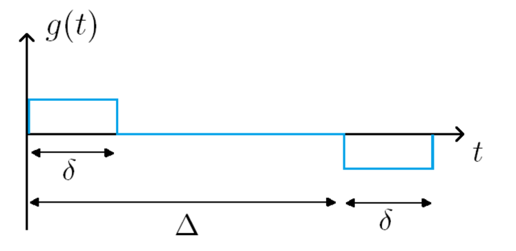
Figure 1: Schematic representation of the pulsed-gradient spin-echo (PGSE) sequence with two rectangular gradient pulses of amplitude $g$ and conventional notations $\delta$ and $\Delta$ for the pulse and inter-pulse durations [56, 57]. The second negative gradient pulse accounts for the refocusing effect of a $180^{\circ}$ rf pulse. While the paper is mainly focused on the particular case $\Delta=\delta$, the localization regime can also be observed and analyzed for $\Delta>\delta$ given that the pulse duration $\delta$ is long enough [53]. In Sec. 4.3, the localization regime is also compared with the opposite setting of narrow gradient pulses ($\delta\to 0$).

In 1991, Stoller, Happer and Dyson have solved exactly the Bloch-Torrey equation (1) in one dimension and predicted the emergence of the localization regime, in which the signal decays much slower at high extended gradient pulses [14]

$$-\log S\propto g^{2/3}\;.$$ (4)

This first non-perturbative approach to the Bloch-Torrey equation was later extended by de Swiet and Sen [45] and validated experimentally by Hürlimann et al. [46]. The mathematical complexity of the seminal paper [14] and the unusual, non-intuitive behavior of the signal led to a common view onto the localization regime as a sort of pathologic anomalous exception. Over many years, these three papers remained under-cited and largely ignored. Only recently, the interest to the localization regime has been revived. The recent works have shown that, as opposed to a common belief, the localization regime is not an exception, but a universal mathematical feature of the Bloch-Torrey equation [47, 49, 48, 50, 51, 52, 53, 54]. Moreover, the high sensitivity of the signal to the microstructure at strong gradients presents an unexplored opportunity for new imaging modalities [55]. Yet, the lack of simple, intuitive description of the localization regime may present a severe obstacle for these exciting developments.

In this paper, we fill this gap and provide a relatively simple yet rigorous explanation of the localization regime and its fascinating properties. We also discuss limitations of earlier proposed hand-waving arguments employed to explain the localization regime. After this didactic presentation, we summarize the panorama of different regimes and their relevance to experiments. Finally, we argue on the universal character of the localization regime, urge for the development of a non-perturbative theory of diffusion NMR, and speculate about future perspectives.

2 Relevant length scales of diffusion NMR

For the sake of simplicity, we will consider the basic Stejskal-Tanner pulsed-gradient spin-echo sequence [56, 57] with two rectangular gradient pulses, each of amplitude $g$ and duration $\delta$, and without inter-pulse time (i.e., $\Delta=\delta$, see Fig. 1). To focus on the effects of diffusion-sensitizing gradients, we ignore $T_{1}/T_{2}$ relaxations, surface relaxation, permeability, susceptibility-induced internal gradients, Eddy currents, and other experimental features which usually superimpose with the considered attenuation mechanism and further complicate the analysis. We will comment on them at the end of the paper.

Following [46], we introduce two length scales in order to distinguish different diffusion NMR regimes: a diffusion length $\ell_{\mathrm{d}}=\sqrt{D_{0}t}$ (with $t=2\delta$) and a gradient length $\ell_{g}=D_{0}^{1/3}G^{-1/3}$, where we set a shortcut notation $G=\gamma g$ for the gradient of the Larmor frequency (see A for a qualitative explanation of the gradient length scale). For free diffusion, there is no other length scale, and the signal attention must be a function of the ratio $\ell_{\mathrm{d}}/\ell_{g}$. Indeed, one finds [58]

$$S=\exp\bigl{(}-\tfrac{1}{12}D_{0}G^{2}t^{3}\bigr{)}=\exp\bigl{(}-\tfrac{1}{12}(\ell_{\mathrm{d}}/\ell_{g})^{6}\bigr{)}$$ (5)

that also justifies the introduction of the $b$-value (here, $b=\tfrac{1}{12}G^{2}t^{3}$, compare with Eq. (2)) as a unique parameter representing the diffusion-encoding sequence.

In turn, the microstructure of a medium (such a brain tissue or a porous sedimentary rock) is usually incorporated via boundary conditions to Eq. (1) and introduces its own length scale(s), denoted as $\ell_{\mathrm{s}}$, resulting in much more sophisticated dependences of the signal on the experimental parameters [59]. When the gradient amplitude $G$ (or $g$) increases, the gradient length $\ell_{g}$ decreases and can eventually become the smallest length scale of the problem. In this case, the transverse magnetization becomes very small everywhere in the bulk, except for a boundary layer of width $\ell_{g}$ near the points where the gradient direction is perpendicular to the boundary (Fig. 2). The residual magnetization localized in these specific regions produces the spin-echo signal, which exhibits the “anomalous” decay (4), as we discuss below. While this common description of the localization regime sounds plausible, an appropriate physical explanation of this phenomenon is still missing, apart from the thorough mathematical analysis of the Bloch-Torrey equation.

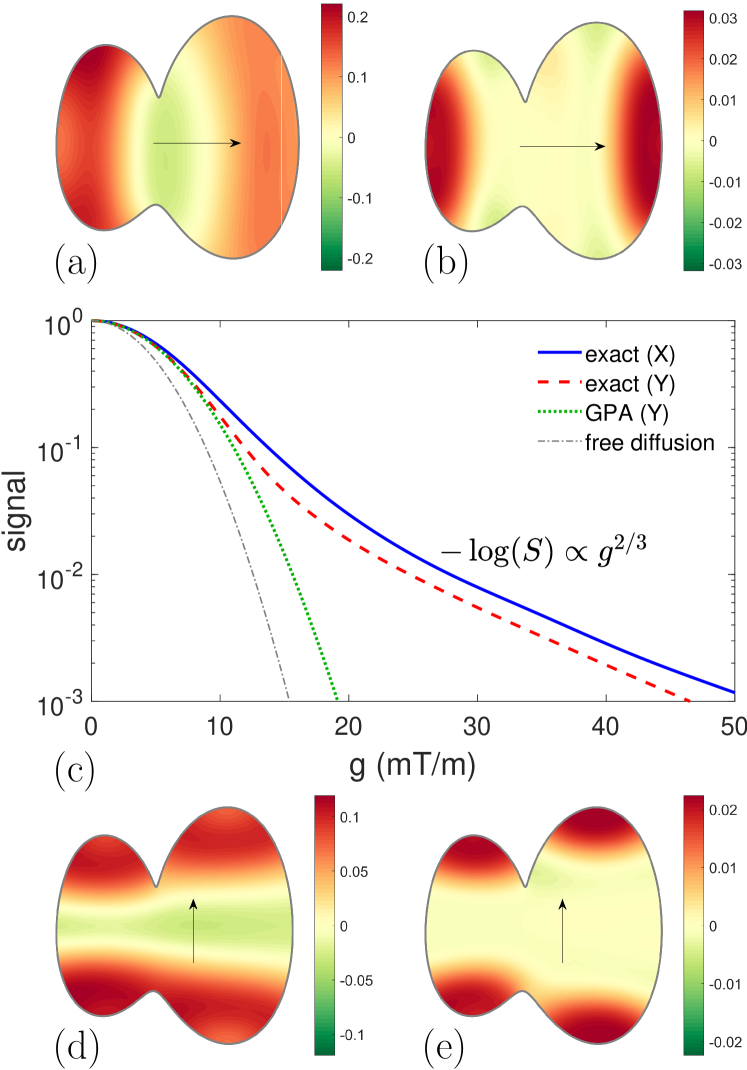
Figure 2: Emergence of the localization regime in a bounded domain with reflecting boundary filled with xenon gas. (a,b,d,e) The real part of the transverse magnetization $m(t,\mathbf{r})$ at the echo time $t=2\delta$ after the second rectangular gradient pulse shown on Fig. 1, with $\Delta=\delta=6$ ms, $D_{0}=3.7\cdot 10^{-5}$ m²/s, $\gamma=7.4\cdot 10^{7}$ s^-1 T^-1, and the linear size of the domain $\ell_{\mathrm{s}}=3$ mm. Panels (a,b) correspond to the horizontally oriented gradient of amplitude $g=15$ mT/m (a) and $g=30$ mT/m (b); Panels (d,e) correspond to the vertically oriented gradient of amplitude $g=15$ mT/m (d) and $g=30$ mT/m (e). In this setting, one has $\ell_{\mathrm{d}}/\ell_{\mathrm{s}}=0.157$, while $\ell_{g}/\ell_{\mathrm{s}}=0.107$ for $g=15$ mT/m and $\ell_{g}/\ell_{\mathrm{s}}=0.085$ for $g=30$ mT/m. One clearly observes the “pockets” of localized magnetization. (c) The spin-echo signal $S$ as a function of the gradient. Solid and dashed lines show the signals $S_{x}$ and $S_{y}$ when the gradient is directed either along the $x$ axis, or along the $y$ axis, respectively. Dotted line indicates the Gaussian phase approximation (3) with $D=2.39\cdot 10^{-5}$ m²/s obtained from a linear fit of $-\log(S_{y})$ versus $b$-value at small $b=\tfrac{2}{3}\gamma^{2}g^{2}\delta^{3}$ (a similar curve with $D=2.19\cdot 10^{-5}$ m²/s obtained from $S_{x}$ is not shown). Thin dash-dotted line presents the free diffusion signal in Eq. (5). The signal and the magnetization profiles were calculated via a matrix formalism based on the Laplacian eigenmodes computed numerically in Matlab PDEtool, see [8, 60].

3 Why does the magnetization localize?

In this section, we aim at explaining why does the magnetization localize at high gradients and how does the gradient length $\ell_{g}$ determine its spatial extent. We will first revise common misconceptions and then provide a qualitative explanation for this behavior. Then we extend this description to emphasize the difference between the motional-narrowing and localization regimes. For clarity, we consider one-dimensional settings, which can be seen as a zoom of the local behavior of the magnetization in the orthogonal direction to the boundary in three dimensions. This qualitative picture is justified by the fact that the gradient length $\ell_{g}$ is supposed to the smallest scale of the problem. Even though the exact solution of the Bloch-Torrey equation in terms of infinite series over Airy functions is known for one-dimensional domains [14, 47], our goal here is to provide a simple, intuitively appealing description of the localization phenomenon.

3.1 Reduced mean-squared displacement?

The main argument that is commonly put forward to rationalize localization of the magnetization is that the displacement of particles along the gradient direction is the most reduced at boundaries that are perpendicular to the gradient. Although this restriction is indeed present, we argue that its effect is far too weak to explain the drastic change in the signal decay in comparison to free diffusion. For a particle diffusing on a half-line $(0,\infty)$ with reflections at the endpoint $0$, the mean-squared displacement can be easily found as

$$\mathbb{E}\{(x_{t}-x_{0})^{2}\}=2\ell_{\mathrm{d}}^{2}\bigl{(}1+f(x_{0}/\ell_{\mathrm{d}})\bigr{)},$$ (6)

where $x_{0}$ is the starting point, and

$$f(u)=u^{2}\left[1-\mathrm{erf}(u/2)\right]-\frac{2u}{\sqrt{\pi}}\exp(-u^{2}/4),$$ (7)

with $\mathrm{erf}(z)$ being the Gauss error function. The correction term $f(u)$ is illustrated on Fig. 3, which reveals that the mean-squared displacement is reduced at most by $40\%$ of its nominal value $2\ell_{\mathrm{d}}^{2}=2D_{0}t$ for free diffusion. Although this is a strong effect in itself and may result, for instance, in the edge enhancement [61], it cannot explain the “anomalous” scaling of the signal in Eq. (4), which is drastically different from the monoexponential law (3) with the characteristic dependence $-\log S\propto g^{2}$. In fact, this argument can justify the reduction of $D_{0}$ to an effective diffusion coefficient $D=D_{0}(1+f(x_{0}/\ell_{\mathrm{d}}))$ but does not break the conventional decay (3). Therefore, this explanation fails to rationalize the localization regime.

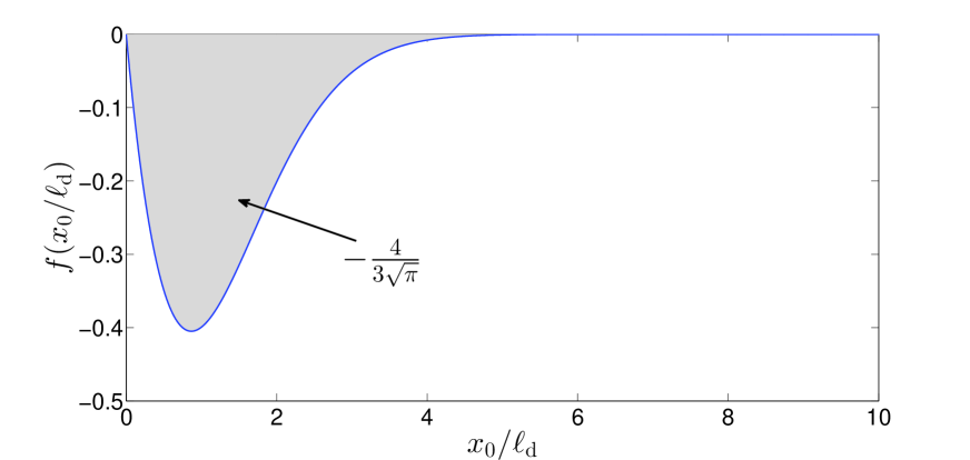
Figure 3: The correction term $f(x_{0}/\ell_{\mathrm{d}})$ given by Eq. (7) that quantifies the relative decrease in the one-dimensional mean-squared displacement from Eq. (6) due to reflections on the boundary, as a function of the starting position $x_{0}$. This is also the relative reduction in the effective diffusion coefficient for particles started from $x_{0}$. The shaded area represents the integral of this correction term over $x_{0}$ and yields the numerical prefactor $4/(3\sqrt{\pi})$ that was first computed by Mitra et al. in the context of diffusion NMR [18, 19]. The fact that the integral is finite expresses that the correction is a boundary effect.

From another viewpoint, the argument of “reduced displacement” still relies on the Gaussian phase approximation, in which the signal attenuation is directly related to the variance of the phase and in turn to the mean-square displacement of particles. However, the distribution of phases is not Gaussian anymore close to a boundary because of velocity correlations introduced by reflections on the boundary.

Another flaw in this reasoning is that the relevant scale here is $\ell_{\mathrm{d}}$ and not $\ell_{g}$. Indeed as shown on Fig. 3, the mean-squared displacement is reduced inside a layer of thickness $\ell_{\mathrm{d}}$ close to the boundary (i.e., for particles started between $0$ and $\simeq 4\ell_{\mathrm{d}}$, see the shaded area). Naturally, one could argue that in the regime of $\ell_{\mathrm{d}}\gg\ell_{g}$, particles that travel further than $\ell_{g}$ would yield a magnetization too small so that we discard them from the computation of the signal. This observation is the basis of the next argument.

3.2 Competition between confined trajectories and magnetization decay?

Let us consider a single impermeable boundary at $x=0$ and introduce a virtual boundary at $x=\ell$ that particles can freely cross. The number of particles $n(\ell)$ that remain confined between the two boundaries during the whole gradient sequence can be estimated as

$$n(\ell)\sim\ell\exp\left(-\frac{\pi^{2}\ell_{\mathrm{d}}^{2}}{4\ell^{2}}\right)\;,$$ (8)

and the (non-normalized) signal resulting from those particles follows from the motional narrowing regime in a slab of width $\ell$ under the hypothesis $\ell\ll\ell_{\mathrm{d}}$ [21]:

$$s(\ell)=n(\ell)\exp\left(-\frac{\ell^{4}\ell_{\mathrm{d}}^{2}}{120\ell_{g}^{6}}\right)\;.$$ (9)

Then one evaluates the competition between motional narrowing decay and “leakage” of particles outside the virtual slab by maximizing the signal with respect to $\ell$. The maximum is achieved at $\ell\approx 2.3\,\ell_{g}$, and the signal becomes

$$s(\ell)\sim\ell_{g}\exp\left(-0.70\,\ell_{\mathrm{d}}^{2}/\ell_{g}^{2}\right).$$ (10)

Although the numerical coefficient $0.70$ is wrong (see below), this simple reasoning provides the correct form of the signal, i.e., $-\log s\propto g^{2/3}$. It shows that the signal is produced by rare trajectories of particles that stay close to the boundaries of the domain. Indeed, the strong diffusion encoding assumption $\ell_{g}\ll\ell_{\mathrm{d}}$ implies that $n(\ell)/\ell$ is very small for $\ell\sim\ell_{g}$.

This is an elegant idea that brings additional insights into the mechanisms behind the localization regime. However, there are flaws in this argument, apart from technical issues such as the use of the motional narrowing formula (9) for non-impermeable (absorbing) boundaries.

The first one is the use of a virtual perfectly absorbing boundary that allows for leakage from the slab but prevents the entry of particles into the slab from the outside. In that regard, it is hard to give a physical meaning to $s(\ell)$, since the signal inside the slab should take into account neighboring particles that enter through the virtual boundary. One could argue that the particles from the outside are discarded because of their strongly attenuated magnetization. However, this argument fails for two reasons: (i) if $\ell\ll\ell_{g}$, particles that come from a distance $\sim\ell_{g}$ may enter the virtual slab without experiencing a strong decay and therefore they cannot be neglected; (ii) if $\ell\gg\ell_{g}$, particles from the outside have weak magnetization, but so do particles inside, and it is not clear why the former might be neglected with respect to the latter.

However, the most problematic issue is the following: the above reasoning could be applied exactly the same way to any point of the medium, regardless of the presence of a boundary. Instead of considering a virtual boundary close to the impermeable boundary, one could consider two virtual boundaries and compute $s(\ell)$ for this “virtual slab”. The only change is $n(\ell)\sim\exp\left(-\pi^{2}\ell_{\mathrm{d}}^{2}/\ell^{2}\right)$ that in turn yields another numerical coefficient in Eq. (10). This observation emphasizes the aforementioned contradictions about the meaning of $s(\ell)$.

Even though this reasoning yields the correct form of the signal, it does not explain why the magnetization is localized at the boundary. In the next section, we suggest a new qualitative interpretation of the localization regime. We will see some similarities with the above discussion that might explain why this wrong reasoning could yield the correct form of the signal.

3.3 Symmetry breaking and local effective gradient

Now, we present our own qualitative explanation of the localization regime. We will show that the main effect of the boundary is not the reduction of particles displacements but a symmetry breaking. This symmetry breaking produces an effective magnetic field that is not linear with position but has a V-shape. Then we show how localization occurs inside this effective magnetic field.

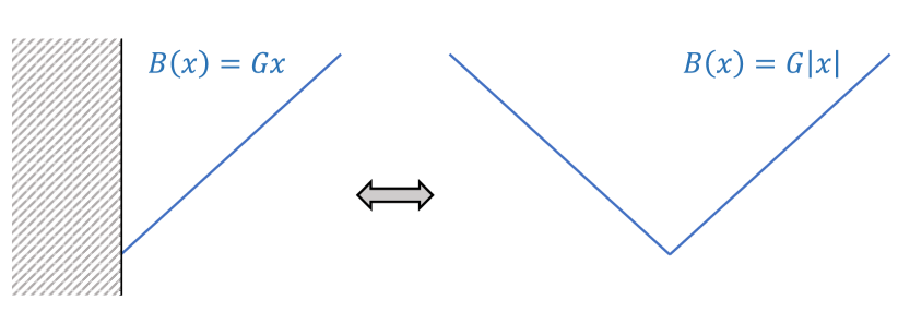
Figure 4: (left) Impermeable boundary and linear magnetic field. (right) No boundary and V-shaped magnetic field. Both situations are equivalent according to the method of images.

For simplicity, we consider again a one-dimensional situation, with an impermeable barrier at $x=0$ and particles diffusing in the half-line $x>0$. The method of images allows one to remove the boundary provided that each particle on the right half-line is paired with a “mirror” particle on the left half-line. Therefore, the effect of the impermeable boundary can be taken into account by replacing the linear magnetic field $B(x)=Gx$ by a V-shape magnetic field $B(x)=G|x|$, as shown on Fig. 4 (a similar effect of a parabolic magnetic field was investigated in [62]). Note that in the Bloch-Torrey equation, the magnetic field plays the role of an imaginary potential, by analogy with the Schrödinger equation. Although it is tempting to make a parallel with localization inside a real potential, it is not evident that the same conclusion would hold for an imaginary potential.

In order to demonstrate the emergence of the localization phenomenon, let us write the magnetization in an amplitude-phase representation, $m(t,x)=A(t,x)e^{i\varphi(t,x)}$, and rewrite the Bloch-Torrey equation (1) in terms of $A$ and $\varphi$:

$$\partial_{t}A=D_{0}A^{\prime\prime}-D_{0}(\varphi^{\prime})^{2}A\;,$$ (11a)

$$\partial_{t}\varphi=D_{0}\varphi^{\prime\prime}+D_{0}\frac{A^{\prime}}{A}\varphi^{\prime}+G|x|\;,$$ (11b)

where prime denotes the derivative with respect to $x$. The initial conditions are $A(t=0,x)=1$ and $\varphi(t=0,x)=0$. The first equation states that $A(t,x)$ obeys a diffusion equation with a reaction rate $D_{0}(\varphi^{\prime})^{2}$. The second equation states that $\varphi$ obeys a diffusion equation with a force term $-D_{0}A^{\prime}/A$ and a source term $G|x|$. We emphasize that $\varphi(t,x)$ is a deterministic function that should not be confused with the random particle dephasing $\phi$.

Short times

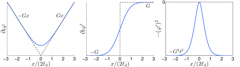
Figure 5: Plot of $\partial_{t}\varphi$ (left), $\partial_{t}\varphi^{\prime}$ (middle), and $-(\varphi^{\prime})^{2}$ (right) at short times ($\ell_{\mathrm{d}}\ll\ell_{g}$).

At short times, $A(t,x)$ is nearly constant and the evolution of the magnetization is dominated by the phase equation

$$\partial_{t}\varphi\simeq D_{0}\varphi^{\prime\prime}+G|x|\;,$$ (12)

whose solution is

$$\varphi(t,x) =G\left[tx\,\mathrm{erf}\biggl{(}\frac{x}{\sqrt{4D_{0}t}}\biggr{)}-\frac{x^{3}}{6D_{0}}\biggl{(}1-\mathrm{erf}\biggl{(}\frac{x}{\sqrt{4D_{0}t}}\biggr{)}\biggr{)}\right.$$

$$\quad\left.+\;\frac{4\;\sqrt{D_{0}t}}{3\sqrt{\pi}}\left(t+\frac{x^{2}}{4D_{0}}\right)\exp\left(-\frac{x^{2}}{4D_{0}t}\right)\right].$$ (13)

The rate of change of $\varphi$ with time can be interpreted as an effective magnetic field averaged by diffusion,

$$\partial_{t}\varphi(t,x)=G\biggl{[}x\,\mathrm{erf}\left(\frac{x}{\sqrt{4D_{0}t}}\right)+\frac{\sqrt{4D_{0}t}}{\sqrt{\pi}}\exp\left(-\frac{x^{2}}{4D_{0}t}\right)\biggr{]}\;,$$ (14)

and the space derivative of this rate of change is an effective gradient averaged by diffusion:

$$\partial_{t}\varphi^{\prime}(t,x)=G\,\mathrm{erf}\left(\frac{x}{\sqrt{4D_{0}t}}\right)\;.$$ (15)

We have plotted these functions on Fig. 5. The main effect of diffusion is to “smooth” the V-potential over a length $\sim\ell_{\mathrm{d}}$ near $x=0$, resulting in a local parabolic shape. In turn, the effective gradient takes smaller values in this region that translates into smaller values of $(\varphi^{\prime})^{2}$. The results for free diffusion are recovered for $|x|\gg\ell_{\mathrm{d}}$, where one gets $\partial_{t}\varphi^{\prime}=G$ and $[\varphi^{\prime}(t,x)]^{2}=(Gt)^{2}$. This limits the validity of the approximate Eq. (12) and its solution in Eq. (13) to short times such that $D_{0}G^{2}t^{3}/3\ll 1$, i.e. $\ell_{\mathrm{d}}/\ell_{g}\ll 3^{1/6}\approx 1.2$. Indeed, these equations rely on the assumption that the amplitude of the magnetization remains approximately constant in space, i.e. that the free diffusion decay far from the boundary is not too strong as compared to the weak decay near $x=0$. This regime corresponds to first two curves with $\ell_{\mathrm{d}}/\ell_{g}=1.0$ and $1.25$ on Fig. 6: the amplitude is practically not affected and the phase profile exhibits the rounded V-shape profile that we just described.

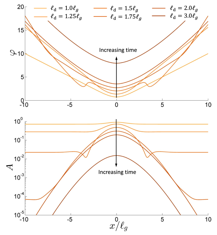
Figure 6: Time evolution of the magnetization in phase (top) and amplitude (bottom) representation, for a constant gradient. The barrier is located at $x=0$ and the amplitude and phase profiles are reflected with respect to $x=0$ according to the method of images. The gradient length $\ell_{g}$ is fixed by the gradient, whereas different curves correspond to six progressively increasing values of $\ell_{\mathrm{d}}$ (as indicated in the legend), which are related to time via $\ell_{\mathrm{d}}=\sqrt{D_{0}t}$. The magnetization $m(t,x)$ was obtained by solving the Bloch-Torrey equation on a long interval $(0,L)$ with reflecting endpoints via the matrix formalism [8, 60]; then its amplitude and phase were computed. We also checked that the numerical solution was in perfect agreement with the exact solution on the half-line derived by Stoller et al. [14]. Refer to the text for further description.

Intermediate times

When the free diffusion decay cannot be neglected anymore, the evolution of the magnetization enters a second stage of intermediate times (next two curves with $\ell_{\mathrm{d}}/\ell_{g}=1.5$ and $1.75$ on Fig. 6). The free diffusion decay term $D_{0}G^{2}t^{3}$ becomes rapidly very large and the amplitude $A$ decays very fast, except at the points where $(\varphi^{\prime})^{2}$ is significantly reduced, i.e. in a thin layer of width $\sim\ell_{\mathrm{d}}\approx\ell_{g}$. As a consequence, the contribution of particles at the sides (with large phase $\varphi$ and small amplitude $A$) is negligible compared to that of particles diffusing from the center, which have small phase $\varphi$ and relatively large amplitude $A$. Thus, the phase profile is broadened by diffusion from the center to the sides, as represented by the force term $(D_{0}A^{\prime}/A)\varphi^{\prime}$. In competition with this broadening effect, the source term $G|x|$ tends to make the phase profile steeper. Since the force term enters through $(D_{0}A^{\prime}/A)\varphi^{\prime}$, there is a value of $\varphi^{\prime}$ at which both effects compensate each other. In parallel, the evolution of the amplitude $A$ in Eq. (11a) results from the competition between diffusion and attenuation. In fact, the inhomogeneous attenuation of the amplitude enhances the effect of diffusion, and in turn diffusion tends to homogenize the amplitude profile. These competing effects may even lead to a non-monotonous dependence of the phase and of the amplitude on $x$ (see the curve with $\ell_{\mathrm{d}}/\ell_{g}=1.5$) but a balance between these two mechanisms is reached after some time. Similarly, the temporal evolution of the phase and the amplitude may be non-monotonous (see, e.g., the curves on Fig. 6 at $x/\ell_{\rm g}\approx 3.5$).

Long times

In the final stage, a dynamic balance between two competing effects is set (two last curves with $\ell_{\mathrm{d}}/\ell_{g}=2.0$ and $3.0$ on Fig. 6). Diffusion tends to broaden the amplitude profile, but the strong decay $-(\varphi^{\prime})^{2}$ destroys the magnetization outside of the region $|x|\lesssim\ell_{g}$. Therefore, the situation is analogous to that of a slab of width $\sim\ell_{g}$ with absorbing boundaries, hence the decay $-\log A\sim\ell_{\mathrm{d}}^{2}/\ell_{g}^{2}$. The source term $G|x|$ tends to make the phase profile steeper but the force term $-D_{0}A^{\prime}/A$ broadens it by “pushing” towards high $|x|$. In other words, particles at the center with a (relatively) strong magnetization diffuse away from the center and outweigh the contribution of particles at the sides that have a much weaker magnetization. Therefore, the source term $G|x|$ contributes only up to $|x|\approx\ell_{g}$, and the phase profile translates upwards as $\sim G\ell_{g}t=\ell_{\mathrm{d}}^{2}/\ell_{g}^{2}$. These conclusions reproduce exactly the behavior of the magnetization in the localization regime.

In analogy to the argument of Sec. 3.2, we obtain that the localization phenomenon at long times is similar to diffusion inside a slab of width $\ell_{g}$ with absorbing boundaries. In other words, the signal in the localization regime is produced by rare trajectories that remain close to the boundary at all times. However, we do not rely on the motional narrowing regime formula and the effect of the boundary is explicitly taken into account as a symmetry breaking of the phase profile: the phase profile becomes even instead of being odd that leads to a region with reduced decay rate $(\varphi^{\prime})^{2}$. In particular, in the absence of a boundary, the magnetic field profile is linear and there is no region of space with a reduced effective gradient, thus no localization.

In the next paragraph, we further emphasize the mechanism of the localization regime by taking into account the size $\ell_{\mathrm{s}}$ of the domain and by investigating qualitatively the transition between the motional narrowing regime and the localization regime.

3.4 Localization regime and motional narrowing regime

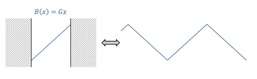
Figure 7: (left) Slab with impermeable boundaries and linear magnetic field. (right) No boundary and periodic triangular profile. Both situations are equivalent according to the method of images.

We employ the same qualitative description as above, but now we consider a finite slab of width $\ell_{\mathrm{s}}$. As illustrated on Fig. 7, the method of images yields a periodic triangular magnetic field, with period $2\ell_{\mathrm{s}}$. To obtain the phase profile $\varphi$ at short times ($\ell_{\mathrm{d}}\ll\ell_{g}$), we solve the diffusion equation (11b) without the force term $(D_{0}A^{\prime}/A)\varphi^{\prime}$ and get

$$\varphi(t,x) \simeq\frac{\ell_{\mathrm{s}}^{3}}{\ell_{g}^{3}}\sum_{n=0}^{\infty}\frac{(-1)^{n}}{4\pi^{4}(n+1/2)^{4}}\sin\left((2n+1)\pi{x}/{\ell_{\mathrm{s}}}\right)$$

$$\times\left[1-e^{-(2n+1)^{2}\pi^{2}\ell_{\mathrm{d}}^{2}/\ell_{\mathrm{s}}^{2}}\right]\;.$$ (16)

The effective magnetic field $\partial_{t}\varphi$ and the effective gradient $\partial_{t}\varphi^{\prime}$ averaged by diffusion follow immediately from this solution and are plotted on Fig. 8. One can see that as time increases, the effective field and gradient become rounder and weaker because of compensation between positive and negative parts. Depending on the range of validity of the above formulas, one is naturally led to distinguish between two regimes. While the transition between these two regimes was rigorously analyzed in [47] by using the exact solution for the magnetization in terms of Airy functions, we provide here much simpler qualitative arguments.

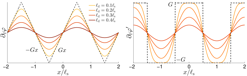
Figure 8: Effective magnetic field (left) and effective gradient (right) averaged by diffusion for $\ell_{\mathrm{d}}\ll\ell_{g}$, at various ratios $\ell_{\mathrm{d}}/\ell_{\mathrm{s}}$. As time increases, both functions become rounder but also weaker because of compensation between positive and negative parts. Note that the slab corresponds to $-1/2\leq x/\ell_{\mathrm{s}}\leq 1/2$ and is repeated periodically according to the method of images.

Localization regime (large slab, strong gradient)

Let us first consider the case $\ell_{g}\ll\ell_{\mathrm{s}}$ corresponding to the localization regime. For example, if $\ell_{g}=0.1\ell_{\mathrm{s}}$, the above formula for $\varphi$ (and its consequences for $\partial_{t}\varphi$ and $\partial_{t}\varphi^{\prime}$) are valid until $\ell_{\mathrm{d}}\lesssim 0.1\ell_{\mathrm{s}}$ (see light yellow curves on Fig. 8). Since $\ell_{\mathrm{d}}\ll\ell_{\mathrm{s}}$, the effective magnetic field profile is close to a triangular shape with small parabolic parts, similarly to the left panel of Fig. 5. The discussion of Sec. 3.3 applies without any modification to this regime, and the magnetization is localized at the boundaries of the slab.

Motional narrowing regime (small slab, weak gradient)

The opposite case $\ell_{\mathrm{s}}\ll\ell_{g}$ corresponds to the motional narrowing regime. In that case, the above formulas for $\partial_{t}\varphi$, $\partial_{t}\varphi^{\prime}$ are valid over a very long time range (corresponding to the dark brown curves on Fig. 8). In particular, for $\ell_{\mathrm{s}}\lesssim\ell_{\mathrm{d}}\ll\ell_{g}$, the phase profile reaches the steady-state form, which is obtained from Eq. (16):

$$\varphi(t,x) \xrightarrow[t\to\infty]{}\frac{\ell_{\mathrm{s}}^{3}}{\ell_{g}^{3}}\sum_{n=0}^{\infty}\frac{(-1)^{n}}{4\pi^{4}(n+1/2)^{4}}\sin\big{(}(2n+1)\pi{x}/{\ell_{\mathrm{s}}}\big{)}$$

$$=\frac{\ell_{\mathrm{s}}^{3}}{24\ell_{g}^{3}}\frac{x}{\ell_{\mathrm{s}}}\left(3-4\frac{x^{2}}{\ell_{\mathrm{s}}^{2}}\right)\quad\bigl{(}-\tfrac{1}{2}\leq x/\ell_{\mathrm{s}}\leq\tfrac{1}{2}\bigr{)}\;.$$ (17)

This expression gives immediately the decay rate,

$$D_{0}[\varphi^{\prime}]^{2}\approx\frac{1}{64}\frac{D_{0}\ell_{\mathrm{s}}^{4}}{\ell_{g}^{6}}\left[1-\left(\frac{2x}{\ell_{\mathrm{s}}}\right)^{2}\right]^{2}\;,$$ (18)

while its average over the half-period,

$$\frac{1}{\ell_{\mathrm{s}}}\int_{-\ell_{\mathrm{s}}/2}^{\ell_{\mathrm{s}}/2}D_{0}[\varphi^{\prime}(t,x)]^{2}\,\mathrm{d}x\approx\frac{D_{0}\ell_{\mathrm{s}}^{4}}{120\ell_{g}^{6}}\;,$$ (19)

yields an average signal decay

$$S\approx\exp\left(-\frac{1}{120}\ell_{\mathrm{d}}^{2}\ell_{\mathrm{s}}^{4}/\ell_{g}^{6}\right),$$ (20)

which is the exact result for the motional narrowing regime [21, 22, 8].

At long times, the decay of the signal becomes significant, and one may wonder about the validity of the above result. Actually, one can see that the decay of the signal occurs on a time scale $\ell_{g}^{6}/(D_{0}\ell_{\mathrm{s}}^{4})$ much larger than the diffusion time scale $\ell_{\mathrm{s}}^{2}/D_{0}$. As a consequence the diffusion term Eq. (11a) flattens any inhomogeneity in the amplitude profile. In turn, since the amplitude profile is nearly homogeneous at all times, the formula (17) for $\varphi$, that relied on neglecting the force term $D_{0}A^{\prime}/A$, is always valid at long times.

3.5 Breakdown of the Gaussian phase approximation

The motional narrowing regime may be obtained from the central limit theorem applied to successive explorations of a bounded domain [22]. The main hypothesis behind this reasoning is that any particle “loses memory” of its initial position after a time $\sim\ell_{\mathrm{s}}^{2}/D_{0}$. This hypothesis allows one to treat the accumulated phases over successive explorations of the domain as independent from each other, that is a crucial assumption of the central limit theorem. This argument implies that the distribution of the random phase $\phi$ is Gaussian, whereas the signal, which can be understood as a characteristic function $\phi$, is a Gaussian function of the gradient strength: $-\log S\sim G^{2}\ell_{\mathrm{s}}^{4}t/D_{0}$. Since this reasoning relies on the central limit theorem, it seems very robust and it is a priori not clear why it would break down if the gradient length is much smaller than the pore diameter (i.e., $\ell_{g}\ll\ell_{\mathrm{s}}$).

The above computation reveals that in the localization regime, a small fraction of particles, of order of $\exp(-\ell_{\mathrm{d}}^{2}/\ell_{g}^{2})$, remains close to the boundary and dominates the signal due to the local symmetry breaking caused by the boundary. In terms of accumulated phase, this means that the velocity correlations introduced by the boundary make the phase distribution non-Gaussian for particles close to the boundary, and its contribution dominates in the signal at high gradients. It is worth noting, however, that the regime $\ell_{g}\ll\ell_{\mathrm{s}}\ll\ell_{\mathrm{d}}$ would yield a very weak signal anyway.

4 Discussion

4.1 Universal character of the localization regime

The simple explicit form (5) of the signal for free diffusion is the first result that a student learns about diffusion NMR. Its natural extension into Eq. (3) via the Gaussian phase approximation, which is always valid at small gradients, and numerous experimental observations re-enforce the common belief that the monoexponential form (3) is the good starting point to analyze signals at higher gradients. On one hand, there are various models based on Eq. (3); on the other hand, the cumulant expansion aims at improving the Gaussian phase approximation by adding perturbative corrections. In this light, the unusual, $G^{2/3}$-behavior of the signal in the localization regime looks indeed as a pathology, far apart from the common trend. In this section, we briefly describe the major flaws of this dogmatic view and emphasize on the universal character of the localization regime.

The non-perturbative approach to diffusion NMR, initiated by Stoller et al. [14] and then developed in a series of publications [45, 46, 47, 49, 48, 55, 50, 51, 52, 53, 54], relies on the spectral analysis of the Bloch-Torrey operator, ${\mathcal{B}}_{g}=-\nabla^{2}+i\ell_{g}^{-3}x$, where $x$ is the coordinate along the gradient direction. For a pulsed-gradient spin-echo sequence shown on Fig. 1, this operator governs the time evolution of the transverse magnetization. If the spectrum of ${\mathcal{B}}_{g}$ is discrete, the signal can be represented as a spectral expansion:

$$S=\sum\limits_{j,k}c_{j,k}(\ell_{g},\Delta-\delta)\,\exp\bigl{(}-(\lambda_{j}(\ell_{g})+\lambda_{k}^{*}(\ell_{g}))D_{0}\delta\bigr{)},$$ (21)

where $\lambda_{j}(\ell_{g})$ are the eigenvalues of ${\mathcal{B}}_{g}$, and $c_{j,k}(\ell_{g},\Delta-\delta)$ are the coefficients based on its eigenfunctions [45, 47]. Since the Bloch-Torrey operator is not Hermitian, the eigenvalues are in general complex-valued: their real part determines the decay of the signal whereas the imaginary part is responsible for eventual oscillations. At high gradients, the eigenvalues exhibit a universal scaling behavior:

$$\mathrm{Re}(\lambda_{j}(\ell_{g}))\propto\ell_{g}^{-2}\biggl{(}1+O\bigl{(}(\ell_{\rm s}/\ell_{g})^{\frac{1}{2}}\bigr{)}\biggr{)}\quad\textrm{as}~{}\ell_{g}\to 0.$$ (22)

For extended gradient pulses (when $\delta$ is large enough), the term containing the eigenvalue $\lambda_{1}$ with the smallest real part provides the major contribution to the signal:

$$S \approx c_{1,1}(\ell_{g},\Delta-\delta)\,\exp\bigl{(}-2\mathrm{Re}(\lambda_{1}(\ell_{g}))D_{0}\delta\bigr{)}$$

$$\sim\exp\bigl{(}-|a^{\prime}_{1}|\ell_{\mathrm{d}}^{2}/\ell_{g}^{2}\bigr{)}=\exp\bigl{(}-2|a^{\prime}_{1}|D_{0}^{1/3}G^{2/3}\delta\bigr{)},$$ (23)

where $|a^{\prime}_{1}|\approx 1.0188$ is a universal numerical prefactor. As we discussed earlier, this behavior is tightly related to the localization of the associated eigenfunctions near the boundary points, at which the gradient is perpendicular to that boundary. The universality of Eq. (23) follows from the local character of this localization phenomenon: when the gradient length $\ell_{g}$ is the smallest scale of the problem, the boundary looks flat on this scale. The effect of other terms in Eq. (21) and the next-order corrections to the eigenvalues are discussed in [53].

As one can see, the above $G^{2/3}$-behavior of the signal is very general, whenever the spectrum of the Bloch-Torrey operator is discrete. This is true for any bounded domain, i.e., when the nuclei diffuse within a finite-size sample. Unexpectedly, the recent works have shown that the spectrum is also discrete for a large class of unbounded and periodic domains [51, 52, 53, 54]. This is a counter-intuitive result because the spectrum of the Laplace operator, ${\mathcal{B}}_{0}=-\nabla^{2}$, which is obtained in the limit of no gradient, is continuous in these domains. In other words, the limit $g\to 0$, in which the discrete spectrum of the Bloch-Torrey operator ${\mathcal{B}}_{g}$ transforms into the continuous spectrum of ${\mathcal{B}}_{0}$, is singular. This general mathematical argument implies that a perturbative construction of the signal that starts from the purely diffusive operator ${\mathcal{B}}_{0}$ and treats the extended gradient pulse as a perturbation, is doomed to fail in such unbounded or periodic domains. Even though this discussion may sound rather abstract, it reveals some fundamental mathematical flaws in commonly used perturbative theories of diffusion NMR and urges for new developments in this field.

Even for bounded domains, the non-Hermitian character of the Bloch-Torrey operator makes the study of diffusion NMR challenging but very rich. In particular, the spectrum of the Bloch-Torrey operator in bounded domains typically has branching or bifurcation points, i.e., there are critical values of the gradient $G$, at which two eigenvalues coalesce. This effect was first discussed by Stoller et al. [14] for an interval and later found in other domains [53, 54]. From the mathematical point of view, such branching points induce non-analyticity in the spectrum and potentially in other related quantities such as the magnetization and the signal. In particular, the cumulant expansion may diverge beyond the smallest critical gradient that would be the ultimate range of validity of a perturbative approach. Further understanding of the limitations of the cumulant expansion presents an interesting perspective for future research.

Anticipating further mathematical progress in this direction, we conjectured that the spectrum of the Bloch-Torrey operator is discrete for any nontrivial domain [55]. If this conjecture will be proved, the general spectral representation (21) and the consequent localization regime at high extended gradients will become a common rule, whereas the free diffusion signal (5) will be an exception from that rule. However, we hasten to stress that such a paradigm shift in the theoretical description of diffusion NMR does not diminish the importance of the Gaussian phase approximation and the related models developed at small gradients. On the contrary, bridging the small-gradient and high-gradient asymptotic forms of the signal presents one of the major theoretical challenges for future research.

4.2 Summary of diffusion NMR regimes

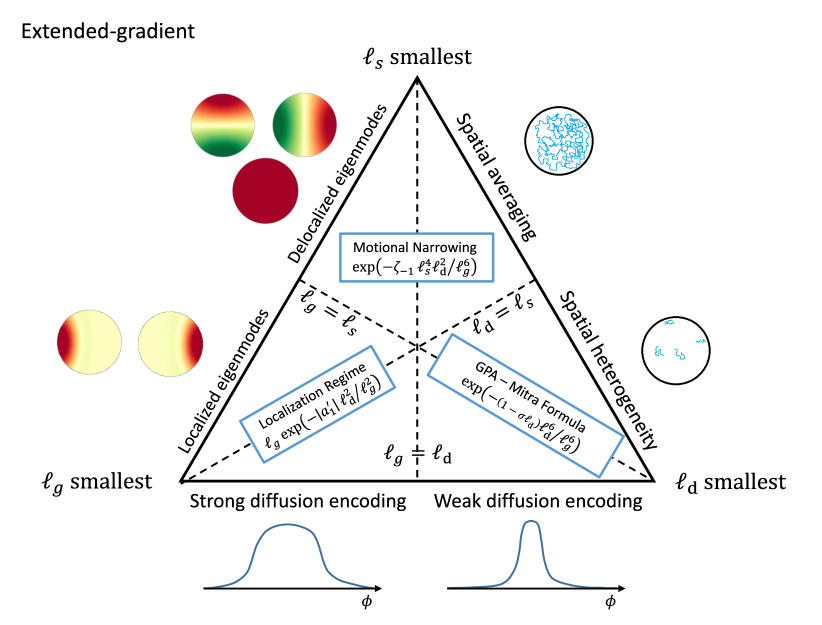
Figure 9: Schematic representation of three regimes of diffusion NMR for extended-gradient pulse experiments. Three length scales $\ell_{\mathrm{d}}$, $\ell_{\mathrm{s}}$ and $\ell_{g}$ are defined in the text. In addition, $\sigma$ is related to the surface-to-volume ratio of the medium [18, 19, 20], $\zeta_{-1}$ is a shape-dependent coefficient [8], and $|a^{\prime}_{1}|\approx 1.0188$ is a universal numerical prefactor [14]. Colored patterns inside the disks on the left illustrate the localized and delocalized eigenmodes of the Bloch-Torrey operator governing the evolution of the transverse magnetization [53, 54].

The above discussion clarified the opposite effects of diffusion and gradient encoding onto the magnetization. The competition of these two effects, characterized respectively by the length scales $\ell_{\mathrm{d}}$ and $\ell_{g}$, produces a variety of diffusion NMR regimes [64, 8]. Hürlimann et al. identified three major regimes by plotting a schematic diagram in the parameters’ plane $(\ell_{g}/\ell_{\mathrm{s}},\ell_{\mathrm{d}}/\ell_{\mathrm{s}})$ [46] (see also [8]). As each of these regimes emerges when one of the three length scales ($\ell_{\mathrm{d}}$, $\ell_{\mathrm{s}}$ and $\ell_{g}$) is the smallest, we find convenient to summarize these regimes by a triangle shown on Fig. 9:

(i) When the diffusion length $\ell_{\mathrm{d}}$ is the smallest, the nuclei travel short distances and acquire weak dephasing. This is the slow-diffusion or short-time regime, in which the effective diffusion coefficient $D$ of the nuclei is reduced by the microstructure. The signal attenuation exhibits approximately the monoexponential form (3), whereas some geometric characteristics of the medium such as its surface-to-volume ratio can be estimated [18, 19, 20].

(ii) When the structural length $\ell_{\mathrm{s}}$ is the smallest, the nuclei explore the confining domain and average the magnetic field inhomogeneities. In this motional-narrowing or long-time regime, the Gaussian phase approximation is again valid, and the signal formally admits the monoexponential form [21, 22]. However, the apparent diffusion coefficient $D$ is inversely proportional to $D_{0}$ and strongly depends on the echo time and the confinement scale $\ell_{\mathrm{s}}$.

(iii) When the gradient length $\ell_{g}$ is the smallest, the transverse magnetization is localized near the boundary, the Gaussian phase approximation fails, and the signal exhibits “anomalous” scaling (4).

While the triangular diagram on Fig. 9 gives a panorama of diffusion NMR regimes, it is still a schematic simplification of the complexity and variety of this phenomenon. In fact, most biological or mineral samples exhibit multiple length scales that so different regimes may co-exist or emerge progressively. In addition, surface relaxation $\rho$ or membrane permeability $\kappa$ would further complicate this picture by reducing the magnetization near the boundary either by relaxation or diffusive exchange. Both effects induce their own length scale, either $\ell_{\rho}=D_{0}/\rho$ or $\ell_{\kappa}=D_{0}/\kappa$, which should be included into the analysis, transforming the triangle diagram into a tetrahedron with four length scales. In this way, one can incorporate the signal decay due to the surface relaxation or permeation without gradient encoding [65] but also investigate their coupling [47]. Finally, we focused on the most basic gradient sequence with two equal rectangular pulses, whereas the temporal profile of the gradient sequence can be easily manipulated in experiments. For instance, the application of unequal rectangular pulses led to pore imaging modality [66, 67], while isotropic diffusion weighting and more elaborated encoding schemes brought novel insights onto anisotropy studies [68, 69, 20].

4.3 Localization versus diffusion-diffraction regimes

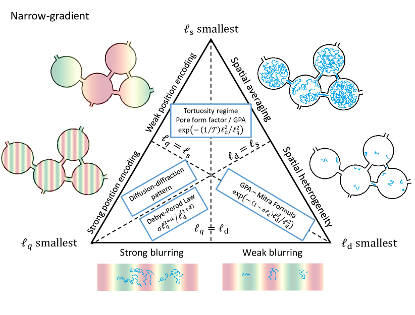
Figure 10: Schematic representation of different regimes of diffusion NMR for narrow-gradient pulse experiments. Three length scales $\ell_{\mathrm{d}}$, $\ell_{\mathrm{s}}$ and $\ell_{q}$ are defined in the text. In addition, $\sigma$ is related to the surface-to-volume ratio of the medium [18, 19, 20], ${\mathcal{T}}=D_{0}/D(t=\infty)$ is the tortuosity of the medium [70], and $d$ is the space dimension. Colored patterns on the left illustrate the phase patterns induced by a narrow-gradient pulse.

High gradient pulses have been employed in diffusion NMR for many decades but they are usually associated with the so-called narrow-pulse approximation [56, 57]. Let us consider again the PGSE sequence shown on Fig. 1. If the gradient duration $\delta$ is very short so that diffusion of the nuclei over time $\delta$ can be neglected, then the effect of a single narrow-gradient pulse is simply to multiply the magnetization by the phase pattern $e^{-i(\mathbf{q}\cdot\mathbf{r})}$ with no attenuation, where $\mathbf{q}=\delta\mathbf{G}$ is the associated wavevector. In turn, the attenuation of the magnetization is caused by the subsequent diffusion step of duration $\Delta$ that “blurs” the phase pattern of period $\ell_{q}=1/|\mathbf{q}|$ (up to a factor $2\pi$). Given that $\delta$ is short, one needs to apply high gradients to reduce $\ell_{q}$ in order to probe the microstructure with comparable length scales. Moreover, the theoretical description relies on the limit of infinitely narrow ($\delta\to 0$) but infinitely strong ($|\mathbf{G}|\to\infty$) gradient pulses with fixed $\mathbf{q}$. The competition between $\ell_{q}$, $\ell_{\mathrm{d}}$ (here, $\ell_{\mathrm{d}}=\sqrt{D_{0}\Delta}$) and the confining length $\ell_{\mathrm{s}}$ yields three major regimes summarized on Fig. 10:

(i) When the diffusion length $\ell_{\mathrm{d}}$ is the smallest, one retrieves the same slow-diffusion regime as with extended gradient pulses in Sec. 4.2.

(ii) When the structural length $\ell_{\mathrm{s}}$ is the smallest, the nuclei explore the confining domain and can thus probe its global structure such as connectivity, tortuosity and disorder [70, 23, 24].

(iii) When the phase pattern period $\ell_{q}$ is the smallest, the blurring of the phase pattern by diffusion renders the signal very sensitive to the microstructure. In particular, the signal exhibits a power law decay (Debye-Porod law) [71, 72, 73], possibly with oscillations (known as diffusion-diffraction patterns), from which some structural properties of the medium can be determined [74, 75, 76, 77, 78].

As for extended-gradient pulses with the smallest $\ell_{g}$, the diffusion-diffraction regime with the smallest $\ell_{q}$ results from the strong coupling between diffusion and gradient encoding and thus potentially allows one to infer fine structural properties. However, such a high sensitivity to the microstructure can also be considered as a drawback: an unavailable variability of shapes and sizes in the microstructure leads to superposition of diffusion-diffraction patterns and may partially or fully destroy them. In this regard, the local behavior of the magnetization for extended-gradient pulses can make the localization regime more robust against such averages, keeping its sensitivity.

Even though both the localization and diffusion-diffraction regimes emerge at high gradients, there are several fundamental differences between them. The signal attenuation occurs due to coupled effects of diffusion and encoding during the gradient pulse in the former case, whereas it is purely blurring effect of diffusion in-between two gradient pulses in the latter case (in particular, if the inter-pulse time $\Delta$ is set to $\delta\approx 0$, there is no signal attenuation). This effect can also be quantified by looking at the $b$-value that characterizes the overall gradient encoding by the pulsed-gradient sequence. Setting $\Delta=\delta$, one gets $b=\tfrac{2}{3}G^{2}\delta^{3}=\tfrac{2}{3}q^{2}\delta\to 0$ in the narrow-pulse limit $\delta\to 0$. In contrast, for extended-gradient pulses with fixed $\delta$, the localization regime corresponds to $G\to\infty$ so that the $b$-value also grows to infinity.

4.4 A practical guideline

To date, there is no experimental protocol exploiting the advantages of the localization regime, notably, its high sensitivity to the microstructure. On one hand, such experiments have to be realized with relatively high signal-to-noise (SNR) ratios, certainly above 10 and better up to 1000. Indeed, as illustrated on Fig. 2 (see also related figures in [47, 53]), deviations from the monoexponential behavior become notable when $S\lesssim 0.1$. In other words, “large” signals decay in a similar (monoexponential) way, whereas the behavior of “small” signals is more specific and thus more sensitive to structural changes. On the other hand, further theoretical progress is needed to handle heterogeneities of the sample such as variability in shapes and sides. While the leading asymptotic term (23) is universal, it is usually not sufficient to accurately describe the signal [53], and one has to resort to the general spectral expansion (21) and to investigate how the spectral properties of the Bloch-Torrey operator are related to the microstructure. An extension to a general temporal profile of the gradient (beyond the considered rectangular gradient pulses) is another important problem for future research.

Even though the advantages of the localization regime are not yet exploitable, the partial localization of the magnetization near the boundaries still affects the signal and may lead to deviations from its monoexponential decay. However, such deviations can also be caused by superposition of signals from isolated pores of variable sizes and shapes, exchange between multiple compartments, surface relaxation or permeation, susceptibility-induced gradients, and other mechanisms. Quite often, non-monoexponential signals are analyzed by fitting to some model formulas, whose adjustable parameters are then related to the microstructure or used as biomarkers. For instance, the bi-exponential model was used to fit the spin-echo signal acquired in the brain, and the estimated fraction of the intracellular space was suggested as a biomarker of cell swelling after an ischemic insult [27]. However, it is important to stress that an accurate fit does not necessarily justify the model underlying the fitting formula [26]. In particular, the bi-exponential model accurately fits the signal shown on Fig. 2(c) for moderate $b$-values but any microstructural interpretation of its parameters is meaningless for this setting. As the origin of the non-monoexponential decay can hardly be identified from a single measurement, it is recommended to conduct a series of experiments by varying the gradient profile, e.g., the amplitude of the gradient pulse, its duration, and the inter-pulse time. An exploration towards high gradients can also be beneficial. When such a systematic investigation is not feasible (e.g., in medical imaging), one can at least estimate the typical length scales $\ell_{\mathrm{d}}$, $\ell_{g}$ (or $\ell_{q}$) and $\ell_{\mathrm{s}}$ in order to position the experimental setting on the diagrams shown on Figs. 9 and 10. Numerical simulations on model structures representative of the studied sample can bring complementary insights.

5 Conclusion

In this paper, we argued about the fundamental importance of the localization regime, which was generally ignored in diffusion NMR. We provided the first qualitative, physically-appealing description of the localization mechanism, beyond a formal mathematical solution of the Bloch-Torrey equation. Contrarily to former hand-waving arguments, we identified the symmetry breaking of the gradient profile by a reflecting boundary as the origin of localization. We emphasized the relation between the “anomalous”, $G^{2/3}$-behavior of the signal, the localization of the transverse magnetization, and the discrete spectrum of the governing Bloch-Torrey operator. Recent mathematical advances in the spectral analysis of this operator support our claim about the universal character of the localization regimes at high extended gradient pulses. In this light, the localization regime is not a pathologic exception but a common rule. Moreover, we discussed fundamental limitations of the current perturbative approaches when the gradient increases. This analysis suggests that the current paradigm in diffusion NMR needs to re-considered towards the development of non-perturbative methods. Quite surprisingly, only now, after seventy years of intensive research in this field, we start to realize how partial is our understanding on the signal attenuation due to the coupled effects of diffusion and magnetic field. In particular, revealing limitations of the cumulant expansion due to branching points of the spectrum and mastering a transition between small-gradient and high-gradient asymptotic regimes remain open problems.

At the same time, the localization regime and related questions are not purely theoretical. An experimental study with a hyperpolarized gas has recently shown the emergence of the localization regime inside cylindrical pores and outside an array of cylindrical obstacles [53]. This study was realized on a clinical MRI scanner and showed severe deviations from the Gaussian phase approximation at gradients as small as 7 mT/m (see also Fig. 2). As a consequence, most diffusion NMR studies nowadays would show such deviations and may be affected by the localization regime. Even though the localization regime is clearly not the only cause of such deviations, its ignorance may result in false and misleading interpretations of experimental results [26, 55]. More generally, the high sensitivity of the signal to the microstructure in the localization regime presents an unexplored opportunity for new imaging modalities. While the weak signal does not still allow one to exploit this opportunity today, further studies of the strong coupling between diffusion and magnetic field encoding will hopefully overcome this practical limitation.

Appendix A Two length scales associated to the gradient

In this Appendix, we elaborate our qualitative discussion about two fundamental length scales associated to the gradient: the gradient length $\ell_{g}$ and the phase pattern period $\ell_{q}$. These two length scales have different physical interpretation and are somewhat “exclusive”: while $\ell_{g}$ is better suited to discuss the behavior of extended-gradient pulse experiments, $\ell_{q}$ is better suited to the opposite case of narrow-gradient pulse experiments.

Gradient length $\ell_{g}$

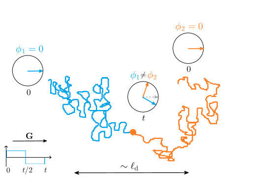
Figure 11: Illustration of diffusion encoding by the gradient. Two particles that meet each other at position $\mathbf{r}$ at the measurement time $t$ have different histories that lead to different accumulated phases $\phi_{1}$ and $\phi_{2}$ (see Eq. (24)). In turn, the resulting phase dispersion leads to signal decay as $S=\mathbb{E}[e^{i\phi}]$.

Let us consider two particles that meet each other at time $t$ at position $\mathbf{r}$. Therefore, they are initially spaced by a distance of the order of the diffusion length $\ell_{\mathrm{d}}=\sqrt{D_{0}t}$ (see Fig. 11). We assume that the pore diameter, $\ell_{\mathrm{s}}$, is much larger than this distance, i.e. $\ell_{\mathrm{d}}\ll\ell_{\mathrm{s}}$, and that the particles diffuse far away from the boundaries of the medium so that we neglect their influence for clarity. Diffusing in a magnetic field gradient $\mathbf{g}(t)$ up to time $t$, a particle acquires the random phase

$$\phi=\int_{0}^{t}\gamma\,\bigl{(}\mathbf{g}(t^{\prime})\cdot\mathbf{r}(t^{\prime})\bigr{)}\,\mathrm{d}t^{\prime},$$ (24)

where $\mathbf{r}(t^{\prime})$ is a random trajectory of the particle. Let $\phi_{1}$ and $\phi_{2}$ denote two realizations of the random phase $\phi$ acquired by two particles. Under a constant gradient amplitude $G=\gamma g$, the random phase difference accumulated by these two particles until they meet is of the order of

$$\left|\phi_{1}-\phi_{2}\right|\sim Gt\ell_{\mathrm{d}}=(\ell_{\mathrm{d}}/\ell_{g})^{3}\;,$$ (25)

where $\ell_{g}=D_{0}^{1/3}G^{-1/3}$ is the gradient length. Equivalently, the variance of $\phi$ at position $\mathbf{r}$ scales as

$$\mathbb{V}[\phi|\mathbf{r}_{t}=\mathbf{r}]\sim D_{0}G^{2}t^{3}=(\ell_{\mathrm{d}}/\ell_{g})^{6}\;.$$ (26)

This quantity describes the phase dispersion at a given position, even if it is position-independent because of the hypothesis of negligible influence of boundaries. If $\ell_{\mathrm{d}}\ll\ell_{g}$ the typical phase difference is small so that the spins have strongly correlated phases. In other words, two different trajectories yield close values of $\phi$ and we call this situation “weak diffusion encoding”. In contrast, if $\ell_{\mathrm{d}}\gtrsim\ell_{g}$, the typical phase difference is large and the spins have almost uncorrelated phases. This is the opposite regime of “strong diffusion encoding” where two different trajectories yield very different values of $\phi$. Therefore, one can interpret the gradient length $\ell_{g}$ as the typical length traveled by particles under the gradient $G$ before they have decorrelated phases with other spins at the same position, provided that they do not reach any boundary.

The above reasoning is still valid if the gradient profile is made of two extended-gradient pulses with no diffusion time in-between them, such as the profile shown on Fig. 1 with $\Delta=\delta$. Indeed, the first (positive) gradient pulse induces a stronger dephasing than the second (negative) one because particles are further apart during the first pulse. However, the argument fails if the pulses are separated by a diffusion time that is significantly longer than the duration of the pulses ($\Delta\gg\delta$). Indeed, the diffusion step with no gradient mixes particles from different areas and thus increases dephasing between spins at a given position. This is especially the case in the narrow-gradient regime where the length $\ell_{q}$, that we describe below, provides more insight into the formation of the signal.

Phase pattern period $\ell_{q}$

The gradient length is an effective way of quantifying the dephasing acquired by diffusing particles because of their random motion, in other words, the variance of $\phi$. In contrast, let us consider the average phase at a given position $\mathbf{r}$ after the first gradient pulse of amplitude $G$ and duration $\delta$, such as on Fig. 1. We assume again that the effect of boundaries can be neglected. As we consider a single constant-gradient pulse, the average value of the random phase $\phi$ is not zero and can evaluated as

$$\mathbb{E}[\phi]=\mathbb{E}\left[\int_{0}^{\delta}\bigl{(}\mathbf{G}(t)\cdot\mathbf{r}(t)\bigr{)}\,\mathrm{d}t\right]=\bigl{(}\mathbf{G}\cdot\mathbf{r}_{0}\bigr{)}\delta\;,$$ (27)

where $\mathbf{r}_{0}$ is the starting point. This implies that the gradient pulse produces a phase pattern with wavevector $\mathbf{q}$ or equivalently with period $\ell_{q}$ (up to a $2\pi$ factor):

$$\mathbf{q}=\delta\mathbf{G}\;,\quad\mathrm{and}\quad\ell_{q}=|\mathbf{q}|^{-1}\;.$$ (28)

Note that in addition to this phase pattern, one should take into account the random dephasing computed above that attenuates the magnetization during the gradient pulse.

Let us consider the limit of infinitely narrow-gradient pulses: $\delta\to 0$ and $\mathbf{q}$ is constant. The above estimation (26) of the variance of $\phi$ just after the pulse shows that it tends to zero in that limit, therefore the effect of a narrow-gradient pulse is simply to multiply the magnetization by the phase pattern $e^{i\mathbf{q}\cdot\mathbf{r}}$ with no attenuation. In other words, the attenuation of the magnetization is solely caused by the subsequent diffusion step of duration $\Delta$ that “blurs” the phase pattern of period $\ell_{q}$.

References

- [1] E. L. Hahn, Spin Echoes, Phys. Rev. 80 (1950) 580–594.
- [2] P. T. Callaghan, Principles of Nuclear Magnetic Resonance Microscopy (Clarendon Press, 1st ed., 1991).
- [3] W. Price, NMR studies of translational motion: Principles and applications (Cambridge Molecular Science, 2009).
- [4] D. K. Jones, Diffusion MRI: Theory, Methods, and Applications (Oxford University Press, New York, USA, 2011).
- [5] D. S. Tuch, T. G. Reese, M. R. Wiegell and V. J. Wedeen, Diffusion MRI of Complex Neural Architecture, Neuron 40 (2003) 885–895.
- [6] J. Frahm, P. Dechent, J. Baudewig and K. D. Merboldt, Advances in functional MRI of the human brain, Prog. Nucl. Magn. Reson. Spectrosc. 44 (2004) 1–32.
- [7] D. Le Bihan and H. Johansen-Berg, Diffusion MRI at 25: Exploring brain tissue structure and function, NeuroImage 61 (2012) 324–341.
- [8] D. S. Grebenkov, NMR survey of reflected Brownian motion, Rev. Mod. Phys. 79 (2007) 1077–1137.
- [9] V. G. Kiselev, Fundamentals of diffusion MRI physics, NMR Biomed. 30 (2017) e3602.
- [10] D. S. Novikov, E. Fieremans, S. Jespersen, and V. G. Kiselev, Quantifying brain microstructure with diffusion MRI: Theory and parameter estimation, NMR Biomed. e3998 (2018).
- [11] H. C. Torrey, Bloch equations with diffusion terms, Phys. Rev. 104 (1956) 563–565.
- [12] E. O. Stejskal and J. E. Tanner, Spin diffusion measurements: Spin echoes in the presence of a time dependent field gradient, J. Chem. Phys. 42 (1965) 288–292.
- [13] D. C. Douglass and D. W. McCall, Diffusion in Paraffin Hydrocarbons, J. Phys. Chem. 62 (1958) 1102–1107.
- [14] S. D. Stoller, W. Happer, and F. J. Dyson, Transverse spin relaxation in inhomogeneous magnetic fields, Phys. Rev. A 44 (1991) 7459–7477.
- [15] D. E. Woessner, NMR spin-echo self-diffusion measurements on fluids undergoing restricted diffusion, J. Phys. Chem. 67 (1963) 1365–1367.
- [16] R. C. Wayne and R. M. Cotts, Nuclear-magnetic-resonance study of self-diffusion in a bounded medium, Phys. Rev. 151 (1966) 264–272.
- [17] E. J. R. van Beek, J. M. Wild, H.-U. Kauczor, W. Schreiber, J. P. Mugler and E. E. de Lange, Functional MRI of the Lung Using Hyperpolarized 3-Helium Gas, J. Magn. Reson. Imaging 20 (2004) 540–554.
- [18] P. P. Mitra, P. N. Sen, L. M. Schwartz, and P. Le Doussal, Diffusion propagator as a probe of the structure of porous media, Phys. Rev. Lett. 68 (1992) 3555.
- [19] P. P. Mitra, P. N. Sen, and L. M. Schwartz, Short-time behavior of the diffusion coefficient as a geometrical probe of porous media, Phys. Rev. B 47 (1993) 8565.
- [20] N. Moutal, I. Maximov, and D. S. Grebenkov, Probing surface-to-volume ratio of an anisotropic medium by diffusion NMR with general gradient encoding, IEEE Trans. Med. Imag. 38 (2019) 2507–2522.
- [21] B. Robertson, Spin-echo decay of spins diffusing in a bounded region, Phys. Rev. 151 (1966) 273–277.
- [22] C. H. Neuman, Spin echo of spins diffusing in a bounded medium, J. Chem. Phys. 60 (1974) 4508–4511.
- [23] D. S. Novikov, E. Fieremans, J. H. Jensen, and J. A. Helpern, Random walks with barriers, Nat. Phys. 7 (2011) 508–514.
- [24] D. S. Novikov, J. H. Jensen, J. A. Helpern, and E. Fieremans, Revealing mesoscopic structural universality with diffusion, Proc. Nat. Acad. Sci. USA 111 (2014) 5088–5093.
- [25] P. J. Basser and D. K. Jones, Diffusion-tensor MRI: theory, experimental design and data analysis-a technical review, NMR Biomed. 15 (2002) 456-467.
- [26] D. S. Grebenkov, Use, Misuse and Abuse of Apparent Diffusion Coefficients, Concepts Magn. Reson. A 36 (2010) 24–35.
- [27] T. Niendorf, R. M. Dijkhuizen, D. S. Norris, M. van Lookeren Campagne and K. Nicolay, Biexponential diffusion attenuation in various states of brain tissue: implications for diffusion-weighted imaging, Magn. Reson. Med. 36 (1996) 847–857.
- [28] R. V. Mulkern, H. Gudbjartsson, C. F. Westin, H. P. Zengingonul, W. Gartner, C. R. Guttmann, et al., Multicomponent apparent diffusion coefficients in human brain, NMR Biomed. 12 (1999) 51–62.
- [29] C. A. Clark and D. Le Bihan, Water diffusion compartmentation and anisotropy at high b values in the human brain, Magn. Reson. Med. 44 (2000) 852–859.
- [30] V. G. Kiselev and K. A. Il’yasov, Is the “biexponential diffusion” bilexponential?, Magn. Reson. Med. 57 (2007) 464–469.
- [31] J. Kärger, NMR self-diffusion studies in heterogeneous systems, Adv. Colloid Interface 23 (1985) 129–148.
- [32] J. Kärger, H. Pfeifer and W. Heink, Principles and applications of self-diffusion measurements by nuclear magnetic resonance, in “Advances in Magnetic Resonance”, ed. J. S. Waugh (Academic Press, San Diego, CA, 1988, vol. 12) 1–89.
- [33] E. Fieremans, D. S. Novikov, J. H. Jensen and J. A. Helpern, Monte Carlo study of a two-compartment exchange model of diffusion, NMR Biomed. 23 (2010) 711–724.
- [34] N. Moutal, M. Nilsson, D. Topgaard, and D. S. Grebenkov, The Kärger vs bi-exponential model: theoretical insights and experimental validations, J. Magn. Reson. 296 (2018) 72–78.
- [35] J. Pfeuffer, S. W. Provencher, and R. Gruetter, Water diffusion in rat brain in vivo as detected at very large b values is multicompartmental, Magn. Reson. Mat. Phys. Biol. Med. 8 (1999) 98–108.
- [36] D. A. Yablonskiy, J. L. Bretthorst and J. J. H. Ackerman, Statistical Model for Diffusion Attenuated MR Signal, Magn. Reson. Med. 50 (2003) 664–669.
- [37] P. T. Callaghan, K. W. Jolley, and J. Lelievre, Diffusion of water in the endosperm tissue of wheat grains as studied by pulsed field gradient nuclear magnetic resonance, Biophys. J. 28 (1979) 133–142.
- [38] D. A. Yablonskiy, A. L. Sukstanskii, J. C. Leawoods, D. S. Gierada, G. L. Bretthorst, S. S. Lefrak, J. D. Cooper and M. S. Conradi, Quantitative in vivo Assessment of Lung Microstructure at the Alveolar Level with Hyperpolarized 3He Diffusion MRI, Proc. Natl. Acad. Sci. U. S. A. 99 (2002) 3111–3116.
- [39] R. L. Magin, O. Abdullah, D. Baleanu and X. Joe Zhou, Anomalous diffusion expressed through fractional order differential operators in the Bloch-Torrey equation, J. Magn. Reson. 190 (2008) 255–270.
- [40] M. Palombo, A. Gabrielli, S. De Santis, C. Cametti, G. Ruocco and S. Capuani, Spatio-temporal anomalous diffusion in heterogeneous media by nuclear magnetic resonance, J. Chem. Phys. 135 (2011) 034504.
- [41] J. H. Jensen, J. A. Helpern, A. Ramani, H. Lu and K. Kaczynski, Diffusional kurtosis imaging: the quantification of non-gaussian water diffusion by means of magnetic resonance imaging, Magn. Reson. Med. 53 (2005) 1432–1440.
- [42] R. Trampel, J. H. Jensen, R. F. Lee, I. Kamenetskiy, G. McGuinness and G. Johnson, Diffusional Kurtosis imaging in the lung using hyperpolarized 3He, Magn. Reson. Med. 56 (2006), 733–737.
- [43] V. G. Kiselev, The cumulant expansion: an overarching mathematical framework for understanding diffusion NMR, in “Diffusion MRI: Theory, Methods and Applications,” ed. D. K. Jones (Oxford University Press: Oxford, 2010, ch. 10).
- [44] D. S. Grebenkov, From the microstructure to diffusion NMR, and back, in "Diffusion NMR of confined systems", Eds. R. Valiullin (RSC Publishing, Cambridge, 2016).
- [45] T. M. de Swiet and P. N. Sen, Decay of nuclear magnetization by bounded diffusion in a constant field gradient, J. Chem. Phys. 100 (1994) 5597–5604.
- [46] M. D. Hürlimann, K. G. Helmer, T. M. de Swiet, and P. N. Sen, Spin echoes in a constant gradient and in the presence of simple restriction, J. Magn. Reson. A 113 (1995) 260–264.
- [47] D. S. Grebenkov, Exploring diffusion across permeable barriers at high gradients. II. Localization regime, J. Magn. Reson. 248 (2014) 164–176.
- [48] D. S. Grebenkov, B. Helffer, and R. Henry, The complex Airy operator on the line with a semipermeable barrier, SIAM J. Math. Anal. 49 (2017) 1844–1894.
- [49] M. Herberthson, E. Özarslan, H. Knutsson, and C.-F. Westin, Dynamics of local magnetization in the eigenbasis of the Bloch-Torrey operator, J. Chem. Phys. 146 (2017) 124201.
- [50] D. S. Grebenkov and B. Helffer, On spectral properties of the Bloch-Torrey operator in two dimensions, SIAM J. Math. Anal. 50 (2018) 622–676.
- [51] Y. Almog, D. S. Grebenkov, and B. Helffer, Spectral semi-classical analysis of a complex Schrödinger operator in exterior domains, J. Math. Phys. 59 (2018) 041501.
- [52] Y. Almog, D. S. Grebenkov, and B. Helffer, On a Schrödinger operator with a purely imaginary potential in the semiclassical limit, Commun. Part. Diff. Eq. 44 (2019) 1542–1604.
- [53] N. Moutal, K. Demberg, D. S. Grebenkov, and T. A. Kuder, Localization regime in diffusion NMR: theory and experiments, J. Magn. Reson. 305 (2019) 162–174.
- [54] N. Moutal, A. Moutal, and D. S. Grebenkov, Diffusion NMR in periodic media: efficient computation and spectral properties, J. Phys. A: Math. Theor. 53 (2020) 325201.
- [55] D. S. Grebenkov, Diffusion MRI/NMR at high gradients: Challenges and perspectives, Microporous Mesoporous Mater. 269 (2018) 79–82.
- [56] E. O. Stejskal, Use of Spin Echoes in a Pulsed Magnetic-Field Gradient to Study Anisotropic, Restricted Diffusion and Flow, J. Chem. Phys. 43 (1965), 3597–3603.
- [57] J. E. Tanner and E. O. Stejskal, Restricted Self-Diffusion of Protons in Colloidal Systems by the Pulsed-Gradient, Spin-Echo Method, J. Chem. Phys. 49 (1968), 1768–1777.
- [58] H. Y. Carr and E. M. Purcell, Effects of diffusion on free precession in nuclear magnetic resonance experiments, Phys. Rev. 94 (1954) 630–638.
- [59] Y.-Q. Song, S. Ryu, and P. N. Sen, Determining multiple length scales in rocks, Nature 406 (2000) 178–182.
- [60] D. S. Grebenkov, Laplacian Eigenfunctions in NMR I. A Numerical Tool, Conc. Magn. Reson. 32A (2008), 277–301.
- [61] T. M. de. Swiet, Diffusive Edge Enhancement in Imaging, J. Magn. Reson. B 109 (1995) 12–18.
- [62] P. Le Doussal and P. N. Sen, Decay of nuclear magnetization by diffusion in a parabolic magnetic field: An exactly solvable model, Phys. Rev. B 46 (1992) 3465–3485.
- [63] D. S. Novikov and V. G. Kiselev, Effective medium theory of a diffusion weighted signal, NMR Biomed. 23 (2010) 682–697.
- [64] S. Axelrod and P. N. Sen, Nuclear magnetic resonance spin echoes for restricted diffusion in an inhomogeneous field: Methods and asymptotic regimes, J. Chem. Phys. 114 (2001) 6878–6895.
- [65] K. R. Brownstein and C. E. Tarr, Importance of Classical Diffusion in NMR Studies of Water in Biological Cells, Phys. Rev. A 19 (1979) 2446–2453.
- [66] T. A. Kuder, P. Bachert, J. Windschuh and F. B. Laun, Diffusion Pore Imaging by Hyperpolarized Xenon-129 Nuclear Magnetic Resonance, Phys. Rev. Lett. 111 (2013) 028101.
- [67] S. Hertel, M. Hunter and P. Galvosas, Magnetic resonance pore imaging, a tool for porous media research, Phys. Rev. E 87 (2013) 030802.
- [68] S. Eriksson, S. Lasic, and D. Topgaard, Isotropic diffusion weighting in PGSE NMR by magic-angle spinning of the q-vector, J. Magn. Reson 226 (2013), 13–18.
- [69] D. Topgaard, Multidimensional diffusion MRI, J. Magn. Reson. 275 (2017), 98–113.
- [70] L. L. Latour, R. L. Kleinberg, P. P. Mitra, and C. H. Sotak, Pore-Size Distributions and Tortuosity in Heterogeneous Porous Media, J. Magn. Reson. A 112 (1995), 83–91.
- [71] P. Debye, H. R. Anderson, and H. Brumberger, Scattering by an Inhomogeneous Solid. II. The correlation function and its application, J. Appl. Phys. 28 (1957) 679–683.
- [72] P. N. Sen, M. D. Hürlimann, and T. M. de Swiet, Debye-Porod law of diffraction for diffusion in porous media, Phys. Rev. B 51 (1995) 601–604.
- [73] A. F. Frøhlich, L. Ostergaard, and V. G. Kiselev, Effect of impermeable boundaries on diffusion-attenuated MR signal, J. Magn. Reson. 179 (2006) 223–233.
- [74] P. T. Callaghan, A. Coy, D. MacGowan, K. J. Packer, and F. O. Zelaya, Diffraction-like Effects in NMR Diffusion Studies of Fluids in Porous Solids, Nature 351 (1991) 467–469.
- [75] P. T. Callaghan, A. Coy, T. P. J. Halpin, D. MacGowan, K. J. Packer, abd F. O. Zelaya, Diffusion in porous systems and the influence of pore morphology in pulsed gradient spin-echo nuclear magnetic resonance studies, J. Chem. Phys. 97 (1992) 651–662.
- [76] A. Coy and P. T. Callaghan, Pulsed gradient spin echo nuclear magnetic resonance for molecules diffusing between partially reflecting rectangular barriers, J. Chem. Phys. 101 (1994) 4599–4609.
- [77] P. T. Callaghan, Pulsed-gradient spin-echo NMR for planar, cylindrical, and spherical pores under conditions of wall relaxation, J. Magn. Reson. A 113 (1995) 53–59.
- [78] P. Linse and O. Söderman, The validity of the short-gradient-pulse approximation in NMR studies of restricted diffusion. Simulations of molecules diffusing between planes, in cylinders, and spheres, J. Magn. Reson. A 116 (1995) 77–86.