Quantifying Performance Changes with Effect Size Confidence Intervals

Abstract

Measuring performance and quantifying a performance change are core evaluation techniques in programming language and systems research. Out of 122 recent scientific papers published at PLDI, ASPLOS, ISMM, TOPLAS, and TACO, as many as 65 included experimental evaluation that quantified a performance change using a ratio of execution times. Unfortunately, few of these papers evaluated their results with the level of rigour that has come to be expected in other experimental sciences. The uncertainty of measured results was largely ignored. Scarcely any of the papers mentioned uncertainty in the ratio of the mean execution times, and most did not even mention uncertainty in the two means themselves. Furthermore, most of the papers failed to address the non-deterministic execution of computer programs (caused by factors such as memory placement, for example), and none addressed non-deterministic compilation (when a compiler creates different binaries from the same sources, which differ in performance, for example again because of impact on memory placement). It turns out that the statistical methods presented in the computer systems performance evaluation literature for the design and summary of experiments do not readily allow this either. This poses a hazard to the repeatability, reproducibility and even validity of quantitative results.

Inspired by statistical methods used in other fields of science, and building on results in statistics that did not make it to introductory textbooks, we present a statistical model that allows us both to quantify uncertainty in the ratio of (execution time) means and to design experiments with a rigorous treatment of those multiple sources of non-determinism that might impact measured performance. Better still, under our framework summaries can be as simple as “system A is faster than system B by 5.5% $\pm$ 2.5%, with 95% confidence”, a more natural statement than those derived from typical current practice, which are often misinterpreted.

Author’s addresses: T. Kalibera (R.E. Jones), School of Computing, University of Kent, Canterbury, CT2 7NF, UK.

A preliminary version of a portion of this work was presented at the Third European Performance Engineering Workshop.

1 Introduction

Quantification of performance change is a common task in experimental computer science. Out of all 122 papers published in ASPLOS, ISMM, PLDI, TACO and TOPLAS in 2011 up to 2nd August, 65 included empirical evaluation that quantified performance change by giving the ratio of execution times (for example, speed-ups of optimisations, or overheads of new techniques). Quantification of performance change is also part of the software development process (for example, detecting performance regressions), both open-source and commercial.

Execution times for quantification are obtained by running benchmark applications using the two systems to compare. Computer systems are becoming more complex and increasingly resemble the direct products of nature observed by physicists and natural scientists — an overwhelming number of factors influence performance. Some are unknown, some are out of the experimenter’s control, and some are non-deterministic. Repeated executions of the same benchmark on the same system, even when the experimenter does everything possible to enforce the same conditions, always report slightly different execution times. This is even more pronounced if the same experiment is repeated by an independent experimenter using different equipment. Thus, for credible quantification of performance change, one needs to design experiments and summarize their results in a repeatable and reproducible manner. Experiment design and statistical inference are the fields of statistics that address these issues, and are widely applied in physics, natural sciences and social sciences.

Unfortunately, the practice in computer science lags behind. Of the 122 papers at ASPLOS, ISMM, PLDI, TACO, and TOPLAS we looked at, 90 evaluated execution time based on experiments. This includes ratio of execution times for two systems and also the execution times for a single system. 71 of these 90 papers completely ignored the question of uncertainty in the measured times. This lack of rigour makes repeatability difficult and undermines the validity of the results. We hardly dare mention that simple rules for summarizing and reporting uncertainties are taught to every student of physics and natural sciences [Kirkup (1994)], are part of engineering practice [Taylor and Kuyatt (1994)], and are based on statistics taught in introductory courses. Moreover, advice on elementary experiment design and statistical inference has been readily available to computer scientists in the form of textbooks aimed and used for teaching [Jain (1991), Lilja (2000)]. A subset of the statistics of the latter textbook has been advocated in the context of Java runtime performance evaluation [Georges et al. (2007)] and compared with the practice in scientific papers, with results not particularly flattering to our field.

Nevertheless, even though the best quantification method recommended so far in our field ([Georges et al. (2007)] based largely on [Lilja (2000)]) is ahead of current practice, it has a number of flaws. It exacts a high price for statistical rigour in summarizing results: we do not get a reliable estimate of the metric that we are ultimately interested in, which is the ratio of execution times. Maybe this flaw on its own is a significant detractor from wider adoption of the method in practice. Even worse, the rigour that the method does provide is highly questionable, as the method is based on statistical significance, a concept with a number of shortcomings, some of which have been known for seven decades [Cohen (1994)]. While statistical significance still dominates elementary statistical textbooks and is still used by some researchers even in other fields, its limits have been well described and arguments for its deprecation have been made in statistics [Royall (1986)], psychology [Cohen (1994)], education [Coe (2002)], ecology, medicine, bio-medicine, and biology [Nakagawa and Cuthill (2007)]. Critical views of statistical significance have also been published in the context of research in sociology, criminology, economics, marketing, chemistry, and nursing (see fidlerps for references and details). Some journals explicitly require alternative methods [Hill and Thompson (2005)]. And such methods are available. As we demonstrate in this paper, the specialized statistical literature  [Fieller (1954), Davison and Hinkley (1997)] provides methods to estimate the ratio of execution times we are interested in — inference of the ratio of means is possible, and a so-called effect size confidence interval can be constructed for it.

Apart from the problems with the summary of results, georges07’s quantification method, while ahead of the prevailing practice in the field, lacks rigour in experimental design. It is based on a two-level  hierarchical experiment that repeats executions of a benchmark, each consisting of repeated measurements. For example, to evaluate an optimisation in a Java virtual machine, the method requires us to run many invocations of the JVM and have each invocation run and measure many iterations of a test application. Two levels are not enough. It is well known that a large number of factors that influence performance are inherently non-deterministic or need to be randomized by experimenter to avoid measurement bias [Mytkowicz et al. (2009)]. The first group includes for example context switches, hardware interrupts, memory placement due to virtual-to-physical memory mapping [Kalibera et al. (2005)], randomized algorithms in compilation [Kalibera and Tuma (2006)], or decisions of a just-in-time compiler on which methods to compile. Non-deterministic compilation by itself means that compilation needs to be repeated. The second group includes symbol names of methods and variables in source code which impacts binary code layout [Gu et al. (2004)], the size of the UNIX process environment or the linking order [Mytkowicz et al. (2009)].

To efficiently run experiments with such as number of sources of non-determinism, we need more than two levels. georges07’s quantification method, however, does not allow this. It is, in fact, based on one-level only summarization, which looks at the means from the lowest level (repeated measurements) instead of the measurement themselves. There is a better way. While not included in elementary statistical textbooks, there are statistical methods which model so-called random effects [Charles E. McCulloch (2008)], which can represent non-deterministic factors in our experiments. To our knowledge, however, none of the existing models can be used directly. Thus, we extend one such model to be more robust and to support an arbitrary number of experiment levels. We also derive the optimum number of repetitions at each level (with the best recommended method so far, there is no systematic guidance to select the number of repetitions).

Our contributions in this work are:

1. Statistical Inference for Quantification. A statistical model of a hierarchy of random effects that contribute to fluctuations in performance. This allows us to build a confidence interval for the mean performance metric (such as execution time) within such a hierarchy. This is our first original contribution to statistics.

2. Experiment Planning for Quantification. After some initial measurements, the model can also be used to guide the experiment. Repeating all experiments blindly is often very expensive. However, the model will give the optimum number of repetitions of experiments at different levels of the hierarchy that are necessary to provide the narrowest confidence interval in available experimentation time. This is our second original contribution to statistics.

3. Asymptotic Parametric Quantification Method. A parametric approach to constructing a confidence interval for the ratio of mean metric values, based on Fieller’s theorem [Fieller (1954)], asymptotic normality of the mean, and our statistical model. Hence, for example, the result of a study might be that the change is 5.5% $\pm$ 2.5%, with 95% confidence. Such a statement provides a clear but rigorous account of the magnitude of the performance change and the uncertainty involved.

4. Bootstrap Quantification Method. An alternative non-parametric approach to constructing the same confidence interval using hierarchical random re-sampling (a bootstrap method). This is an application of an existing statistical method, used in our field much less than it deserves.

5. Evaluation. Thorough evaluation of the two approaches on a set of benchmarks. We estimate the true coverage of the intervals that can be obtained. We also estimate a false alarm rate (the case where a change is detected although there is none), given a threshold of how large changes need to be for us to care. A particularly important benefit of our method is that it supports a rigorous way to use such a threshold. This is our third original contribution.

Contributions 1, 2, 4, and partially 3 and 5 also apply to evaluations of a single system. For contributions 1 and 2, we extend and correct a preliminary version published in [Kalibera and Tuma (2006)], which in turn extends [Kalibera et al. (2005)]. For item 5, we use our benchmark data from [Kalibera and Tuma (2006)] as inputs for (new) statistical simulations.

2 BACKGROUND: Current Quantification Methods

In this section, we provide an overview of quantification methods currently used, we describe their limitations, and we summarize the best-so-far quantification methods recommended for overcoming these limitations.

2.1 Currently Used Methods

To map the current quantification methods used in computer science, we analysed papers published at selected conferences (PLDI, ASPLOS, ISMM) and journals (TOPLAS, TACO). We restricted our survey to papers published between 1st January and 2nd August, 2011. We thus cover all papers from the conferences, issues 1–4 of TOPLAS, and issues 1–2 of TACO — 122 papers in total.

As summarized in Table 2.1, nearly three quarters of the papers studied included empirical performance evaluation that measured and reported execution time. The majority of the execution time evaluations (over 70%) reported the ratio of execution times as a measure of performance change (the remaining 30% reported execution time for a single system). In total, over half of all papers reported the ratio of execution times. We also noted papers where execution time was important for the evaluation (counts in parentheses in the table). More than half of the papers had empirical evaluations with execution time as an important metric. Out of these papers where execution time was an important metric, in nearly 90% it was the ratio of execution times that was reported (only in 10% of cases it was the absolute execution time for a single system). Nearly half of all papers had empirical evaluation with ratio of execution times as an important metric. The ratio of execution times thus seems to be a metric that people care about and report. Anecdotal evidence confirms that this metric is also important to industrial developers.

In practice, where decisions have to be made based on the results of performance quantification, there are certain minimum thresholds for relative performance change above/below which it is considered of no practical interest. These thresholds may depend on the evaluation context (a particular system, regression test, optimisation, new feature). These thresholds are also assumed and used in georges07. Of the papers in our survey, thresholds on ratio of execution times are explicitly part of an auto-tuning algorithm by mapreduce, where they have to be set (manually, based on experience) large enough to cater for variabilities in the data. However, most papers that quantify performance change report only the ratio of (mean) execution times, and thus imply that this ratio alone, maybe along with an understanding of the context of the study, is sufficient to assess importance of a performance change. The use of ‘thresholds’ to assess importance is implied. We also have confirmation from a senior member of a well-known industrial research laboratory of the use of such thresholds in industry.

Current Practice of Performance Quantification PLDI ASPLOS ISMM TOPLAS TACO Total Number of Papers 55 32 13 13 9 122 Evaluated Execution Time 42 (28) 25 (20) 12 (11) 5 (2) 6 (6) 90 (67) Ignored Uncertainty In Measurement 39 (24) 18 (12) 5 (5) 4 (1) 5 (5) 71 (47) Evaluated Ratio of Execution Times 27 (25) 22 (19) 9 (8) 1 (1) 6 (6) 65 (59) Source:Scientific papers at selected venues published in 2011, up to 2nd August. Counts are given in form ‘A (M)’, where A is the number of all papers that reported the metric, and M the number of papers where the metric was important or the main result in the evaluation.

Nearly 80% of the papers studied that evaluated execution time (both absolute and relative) failed to mention anything about uncertainty in the figures they reported. The numbers are not that much better if we only focus on papers where execution time was an important metric: 70% of these papers failed to mention uncertainty. Note that we were very generous in the classification — if a paper reported that uncertainty was low, without any further details, we gave it the benefit of the doubt and counted it as having taken uncertainty into account. Ignoring uncertainty represents a severe lack of rigour in face of the fact that execution time on today’s computer systems is always subject to variation in performance. While majority of the papers studied ran experiments on real hardware, it should be mentioned that some (particularly from ASPLOS) were based on execution time measurements in a simulator. It is certainly possible to have a simulator in which execution time is deterministic, and we did not attempt to check the particular simulators used in individual papers we analysed. However, if a simulator is deterministic, it is not a realistic one [Alameldeen and Wood (2003)]. Thus, we have not attempted to extract simulations from the summary — using a deterministic simulator in our opinion falls into the category of ignoring uncertainty.

We used to hear arguments that, for very large speed-ups (say 2$\times$), summarizing uncertainty is a waste of effort. This implies that experimenter experience is that, in the given system, uncertainty would be much smaller. However, in systems research much smaller performance changes are usually reported. envsize found that out of 88 papers from ASPLOS 2008, PACT 2007, PLDI 2007, CGO 2007 with experimental evaluation in a dedicated section, the median of reported speed-ups was only 10%. In their work they show that the measurement bias with SPEC CPU 2006 benchmarks can easily obfuscate this speed-up when evaluating compiler optimisations. This means proper randomization to avoid this bias would have lead to higher uncertainty than 10%, and hence proper handling of this uncertainty would be necessary (such a randomization tool was later provided by stabilizer). A senior member of a well-known industrial research lab told us that he would care only about differences of 10% for new work, but look for differences of as little as 2-3% or even 1% when looking for regressions (where he would look at uncertainty too). Since such small performance changes are often of interest, ignoring uncertainty in systems research represents a serious threat to validity. When speed-ups are large compared to expected uncertainty, validity would not be threatened, but ignoring it would still be a serious lack of rigour and in our view not a property of good research.

Out of the 19 papers that touched on uncertainty in any way, most reported uncertainty of single systems in the form of a standard deviation or of 95% confidence intervals. It was exceptional for a paper to specify how the confidence intervals were constructed; most were presumably based on the normal distribution. While most papers reported the ratio of execution times, they mostly showed uncertainty only for the means in isolation of each of the two systems compared. Only three of the papers reported the uncertainty of the ratios. However, it seems from the text of two of these that they did not take uncertainty of both systems into account, but only normalized the uncertainty of the new system against the mean of the old system. The third paper was ours, and it took the uncertainty of both systems into account, but we have to admit that our text did not say that. The remaining papers which address uncertainty do so by saying that it was low (without giving numbers), and one says that a proposed optimisation reduced it (without giving numbers).

The papers we studied gave extremely little information on the experimental design used. From some papers, it is not even obvious if benchmarks were executed more than once, and hence if the reported execution time is not just a single measurement. Only very few papers mention that their experiments repeat at two levels (i.e. execution of a benchmark and measurement within that benchmark). However, all of those that do also seem to treat the data as if it came from a one-level experiment. If executions were repeated, the numbers of repetitions seemed to be arbitrary. Some experiments used an adaptive number of iterations based on a heuristic — the benchmark code itself calculates the standard deviation of the last few measurements taken and terminates the experiment once the standard deviation is sufficiently small.

Some papers claim to use certain evaluation methodologies, such as those of envsize, georges07 or georges08. However, these papers rarely made it clear how the concrete experiments were performed. One paper claims to use the method proposed by envsize to reduce variance, without any further details. However, the cited paper argues for dealing with measurement bias through randomization, which in fact increases the variance, but for very good reasons. Some papers mention uncertainty due to the decisions of a just-in-time compiler of which methods to compile. Confidence intervals or standard deviation error bars are usually shown for a single system with one particular configuration, even when multiple configurations were used. Uncertainty quantified in this way is prone to bias.

Summary

The ratio of (mean) execution times is the major metric for quantification of performance change. A threshold for the minimum/maximum ratio is used as a measure of the practical importance of a difference. Uncertainty in the ratio of execution times is almost never quantified, and when it is, only in an unclear way. Sometimes separate uncertainties for the two systems (means) are shown, but more commonly even these are ignored. Benchmarks are mostly repeated only at one level, or exceptionally at two levels (executions and measurements). Two-level experiments, if done at all, are evaluated as if they were one-level only (we believe by merging all the measurements from the different executions, but the texts are not explicit here).

2.2 What Is Wrong With Currently Used Methods

Any paper that reports execution time, yet ignores the uncertainty of the final metric, be it absolute execution time of one system or the ratio of execution times for two systems, is methodologically flawed. Moreover, failing to address uncertainty makes the results unrepeatable. Repeating any experiment will lead to slightly different results due to variability in measurement. Without quantified uncertainty, we cannot know if we got a ‘slightly’ different result due to variability in measurement, or a very different result due to an error. Note that a failure to address uncertainty is not the only way to get unrepeatable results. A common problem is measurement bias, when the experimenter fails to identify and then describe or vary a factor that largely influences the results [Mytkowicz et al. (2009)]. In such a case, statistics even properly used for factors that were varied cannot help and the summarized uncertainty would be misleadingnly small. The responsibility for identifying these factors lies fully on the experimenter and no statistics can help. But even when important factors are fixed and described or varied properly, failing to address uncertainty is a potential threat to validity when quantifying performance change, and this threat is particularly high when the observed change is relatively small (e.g. 10%), which it often is. When such quantification is used to show that an optimisation provides a good speed-up, there is a risk that the ‘improvement’ lies within the range of uncertainty. A similar risk applies to some extent when quantification is used to show that the overhead of a certain feature is small — if the uncertainty of the new system is much larger than the old one, the price may in practice be high even if the mean overhead is small.

Failure to report how many repetitions of a benchmark were executed makes repeatability harder. Often, the reader is only left with suspicion that insufficient repetitions were made and in particular that the researchers did not repeat whole executions of benchmarks (that in turn repeat measurements within a single execution). Sometimes, the reported number of measurements used for averaging is suspiciously small (e.g. three or five). Failure to repeat enough times, or indeed to repeat at all, increases the risk of obtaining unrepeatable results and reaching incorrect conclusions.

In summary, our survey of published papers suggests that the current practice of quantification of performance change in scientific papers is weak. We are not the first to find this, but we were surprised at how prevalent this practice is even in the most recent papers. The lack of reporting of uncertainties while quantifying a performance change in Java runtimes research was documented by georges07. envsize discovered that measurement bias was not addressed in experimental computer systems performance evaluation; this is a more general problem, but it also applies to the quantification of performance change. These shortcomings have arisen despite well-known textbooks on computer systems performance evaluation [Jain (1991), Lilja (2000)] having described a number of errors common in performance evaluation.

2.3 Currently Proposed Methods

Experimental design and statistical inference are mature fields of mathematical statistics with many results and described in a number of texts. Basic recommendations on conducting experiments in physics and natural sciences, measuring uncertainties, calculating propagation of uncertainties, and reporting the results are available in textbooks such as [Kirkup (1994)]. More advanced rules of propagation of uncertainties can be found in a recommendation by NIST [Taylor and Kuyatt (1994)]. High-level overview and pointers to works on experiment design and the scientific method in general can be found in [Wilson (1952)]. While physics does not deal with exactly the same problems as experimental computer science, many ideas are general. Moreover, basic methods of statistical inference and experimental design, in the context of computer systems performance evaluation, have then been presented in books [Jain (1991), Lilja (2000)]. These books have been and are being used as textbooks for teaching performance evaluation courses. georges07 argued for wider adoption of a performance change quantification method based on Lilja’s book, in the context of performance evaluation of Java runtimes. They also added some practical recommendations for the number of repetitions of benchmark measurements.

In this section, we summarize the current recommended best practice for quantification of performance change, based on jain, lilja, and georges07.

2.3.1 Experiment Design

georges07 recommends repeating measurements within a single benchmark, as well as repeating executions of the whole benchmark. The number of measurements within a benchmark is controlled by a heuristic in the benchmark — as soon as the standard deviation of the last few measurements is small enough, the benchmark’s execution is finished. The number of benchmark executions is an arbitrary choice of the experimenter, or, alternatively, additional executions are adaptively added until confidence interval for the mean is sufficiently narrow (its width is within 1% or 2% of the sample mean).

lilja and particularly jain also recommend experimental designs that cope with various combinations of factors that can be fixed by the experimenter. These designs apply to factors that can take only a finite, usually small, number of values (i.e. a particular processor or benchmark). The effect of choosing a particular value (say the processor) on performance is of interest to the experimenter. Such effects are called fixed effects in statistics (see [Charles E. McCulloch (2008)] and [Searle et al. (1992)] for more detailed discussion of fixed and random effects). The experimental designs then help in planning which combinations of values of which factors to run to get reasonable information given reasonable experimentation time. The methods recommended by jain and  lilja, however, do not address effects of factors that can take a large number of values, usually at random and often not under our control, for which the performance effect of a particular choice is not interesting. Such a factor can be, say, a particular mapping of virtual to physical pages chosen by the operating system. In statistics, these are called random effects. In this work, we only address random effects. Our work could be extended to include fixed effects, as there indeed are statistical models that include both types of effects [Charles E. McCulloch (2008)], but we do not attempt it here.

georges08 proposes a particular experiment design for performance evaluations within managed environments with just-in-time compilation. The design assumes generation of several compilation plans and then running both systems using these plans. The motivation for this design, in contrast to just keeping the compilation plans random (unpaired) for the two systems, is smaller uncertainty within given experimentation time.

2.3.2 Summary of Experiment Results

A performance change is quantified using statistical significance [Georges et al. (2007), Lilja (2000), Jain (1991)]. The output is a binary decision: “the systems (may) have the same performance” or “(it is likely that) the systems do not have the same performance”. This decision is based on the probability that the actually observed difference or larger in (sample) means of the two systems would occur if the (true) means were the same. This probability is called the p-value in statistical tests. The p-value is compared against a pre-defined threshold called significance level (i.e. 5%). If the p-value is smaller, then the second decision, that the systems do not perform the same, is chosen. Otherwise, the first decision, the default that they may have the same performance, is chosen.

There are two recommended alternative methods that provide this kind of quantification. The preferred one is a visual test using confidence intervals. The other one is a statistical test. The visual test is as follows. We construct two confidence intervals for the means of the two systems. We check if they overlap. If they do not, the decision is that “it is likely that the systems do not have the same performance”. If they do overlap, the method recommended by lilja and georges07 finishes, concluding that “the systems may have the same performance”. The method by jain adds another step — it falls back to a statistical test if the intervals overlap only slightly, that is if centre of neither interval lies within the other. The visual test is preferred, because in addition to the binary decision, it is easy to give a visual measure of how large the difference in the means actually is, compared to their uncertainty. While this is a clear aid for an analyst, it lacks a rigorous semantics (and in his dissertation,  georgesphd recommends using the statistical test instead).

The confidence interval used for the visual test has the same underlying statistical backing as the statistical test. It is assumed that measurements are independent identically distributed and follow the normal distribution (the normality assumption is incorrectly omitted in many texts as we discuss in greater detail in Section 3.2). jain and lilja suggest using Student’s t-test for unequal variances (or the corresponding interval). georges07 additionally recommend (an interval based on) the z-test for sample sizes over 30. georges07 also suggest working with sample means of measurements from individual executions, instead of with the measurements themselves. The corresponding test/interval is hence only for these sample means. An alternative solution that is sometimes used, but not part of their recommendation, is to join all the measurements from the different executions and treat them as coming from a one-level experiment.

lilja and particularly jain then describe analysis of variance (ANOVA) methods to summarize experiments where multiple fixed factors are varied (i.e. processor, memory size, etc.). georges07 summarizes also some of the ANOVA methods from [Lilja (2000)], but does not recommend it for use in (Java) performance evaluations as the outputs are too hard to understand and doing all the measurements to provide the inputs is too time consuming. We do not address these types of factors (‘fixed effects’) in this work, but our method should be extensible to do so.

The summarisation method that georges08 recommends for the replay compilation design leads to a test/interval based on paired t-test. The inputs are differences of means obtained from the old and new systems, averaging over multiple executions with a given compilation plan. We do not address paired comparisons in this work, but most of our criticism of the recommended quantification using the test/interval we mention later applies to it as well.

3 What Is Wrong With The Currently Proposed Methods

Even though the current recommended best practice for quantification of performance change by [Jain (1991)],  [Lilja (2000)], and [Georges et al. (2007)] is ahead of the pitiful practice in the field, it has a number of problems.

3.1 Experiment Design

Repetition of executions (and measurements) is not enough. It is necessary to include all inherently random factors in the experiment, and hence to repeat experiments at level(s) even higher than execution of the benchmark. For example, randomized compilation necessitates both compilation and running the experiments for different binaries. We have found this to be essential in our earlier work with the GNU C++ Compiler when benchmarking CORBA middleware and when benchmarking applications within the Mono platform  [Kalibera and Tuma (2006)]. The empirical evaluation in this paper confirms this need on the Mono platform. Furthermore, we need to randomize and include additional (non-random) factors that it does not make sense to fix. These factors can arise from the operating system or the language environment. envsize provide evidence that unexpected factors such as the size of UNIX process environment or the linking order can impact performance. verbrugge observed a performance impact of the names of identifiers in the source code. It is obvious that many additional factors of this kind have not yet been discovered to have significant performance impact, so they cannot be really fixed in experiments. Sufficient randomization, called for by envsize, is hence necessary. stabilizer provide a randomization tool applicable to applications studied in [Mytkowicz et al. (2009)].

Note in particular that randomization of identifier names or linking order leads in turn again to randomized compilation/building. Repeating compilation or repeating at an even higher level can be very expensive, because large systems take long to compile. Repeating too many times is a waste of resources, but repeating too few times undermines repeatability and validity. Hence, a good experiment design method should also allow the researcher to derive an optimum number of repetitions at different levels, so as to make efficient use of the time available for experimentation in order to reduce uncertainty in the final result. The present recommended best practice does not offer this.

3.2 Summarization of Experiment Results

The single most significant problem of the best recommended method is that it does not tell us what we want to know. It does not give us the metric we are ultimately interested in, a reliable estimate of the ratio of execution times. Of course, we can use the recommended method and, in the case that the (binary) conclusion is that the systems are likely to differ in performance, we can in addition report the ratio of the sample means. But the recommended method would not give us the uncertainty of this ratio, so we do not know how much of the ratio is due to uncertainty. Since we do not report uncertainty of the ratio, the results we provide are unrepeatable and may not be valid. This problem also means that the recommended method does not allow us to compare the ratio against a threshold (the minimal/maximal change that is important to us).

The problem of not supporting comparison against a threshold is more significant than it may seem at first — the recommended method looks for a performance difference however small as long as it is unlikely to be by pure chance. However, the larger the sample size is (the more measurements we have), the more unlikely even a very small difference becomes. Hence, the decision of the method is influenced by the number of measurements. In practice this means that with a large sample size (and in our field it is easy to generate very large samples), the decision will nearly always be “it is likely that the systems do not have the same performance”, no matter how small or large the difference actually is. The method then becomes of very little use — it just adds an illusion of rigour to the results and, worse, only to the results we are not interested in.

The fact that this does not tell us what we want, and that it often gives the same answer only because the sample size is very large, is a fundamental drawback to the statistical significance. This drawback has been known for the last seven decades [Cohen (1994)]. It has been reiterated by researchers in psychology [Cohen (1994)], education [Coe (2002)], and more recently in bio-medicine and biology [Nakagawa and Cuthill (2007)]. This and other drawbacks of the method have been brought up in criticism of statistical significance also in sociology, criminology, economics, marketing, chemistry, and nursing (see fidlerps for references and details). The drawbacks, however, seem to be quite unknown to experimental computer scientists. Even worse, methods based on statistical significance are notoriously hard to interpret. This may be partially because they do not give us the answer to what we want to know, but they also offer temptations, such as the belief that the p-value is actually the probability that the systems have the same performance. The interpretation of the results of statistical tests is so difficult that even statistical textbooks sometimes get it wrong (examples are given by cohen). In a study by oakes cited by cohen, 68 of 70 psychologists made an error in the interpretation of a statistical test. Interpretation of the visual test using confidence intervals seems simpler, but it is not much so. This is well reflected by the wording used and stressed by lilja, and repeated by georges07 and georges08, to describe the positive outcome (the systems differ in performance) of the visual test — “there is no evidence to suggest that there is not a statistically significant difference”.

The wording is rather cryptic as it tries to be precise, which we do not find it to be. In frequentist statistics which the texts rely on, the wording is incorrect. The goal of the comparison is to learn something about the difference in the true but unknown means of two random variables. The true means are either equal or different, and the statistical significance does not speak about this difference (it speaks about the difference of the sample means instead). Hence, the second part of the wording, “statistically significant difference” is incorrect. The first part of the wording that speaks about non-existence of evidence is incorrect as well. The test is about verifying if the data we have measured are unlikely provided the true unknown means are the same. Hence, we are checking if the data we have form an evidence against the assumed zero performance change. We can make no claims about non-existence of evidence. And we are not looking for evidence for the true means being equal, but rather against it.

lilja (also cited by georges07) explain the wording by stating that there is always a certain probability, ‘$\alpha$’, that a large observed difference was due to random fluctuations. This is correct, but does not justify the wording in our opinion. Even more, the context in the texts suggests that in the visual test of confidence interval overlap, this probability ($\alpha$) is the significance of the confidence intervals used (i.e. $\alpha=0.05$ for 95% confidence interval), which it is not. In fact, with the visual test this probability is not known. If we use 95% confidence intervals, the probability of such an error is not 5%, but under the normality assumption is below 1% [Payton et al. (2003)]. This makes the visual test far more conservative than it may seem, and hence its results are even harder to interpret, and more likely to mislead. Also, one would need far more experimentation time to show a performance change. Further information on the error of the visual test can be found in overlapp,schenker.

With the (non-visual) statistical test, the theory tells us the probability of erroneously concluding that compared systems do not have the same performance when actually they do. The probability of this error is the threshold we are comparing the p-value against (often 5%). For this reason, schenker (cited by georgesphd) prefer statistical test over the visual test. Our understanding is that the visual test is generally preferred, though, in our field, and that both method share their key problems.

Yet another issue of visual and non-visual test is the use of parametric methods on data that violate their assumptions. Computer performance measurements cannot be assumed to be normally distributed. Often they are multi-modal, with long-tails to the right. Deviations from normality may not be fatal for the t-test/confidence interval though, and some practitioners in other fields ignore them as well. The sample mean is asymptotically normal due to the Central Limit Theorem. Many texts in our field omit the normality assumption of the t-test or incorrectly state that the Central Limit Theorem is enough to overcome it ([Lilja (2000), Jain (1991), Georges et al. (2007)]). The Central Limit Theorem is not enough, but some more involved studies show that, under certain deviations from normality, the parametric methods work well, even for reasonably small sample sizes (see for example cfirobust or robustsim) given a reasonably high confidence (95% confidence intervals and wider). Still, there is no general agreement that ignoring the normality assumption is an acceptable practice, one should certainly make it clear if such assumptions are ignored. Robust statistical methods do exist (see robustas for summary and references), and there has been no study of how the t-test/confidence interval is affected by violations from normality common in computer performance data.

4 How to do things better

A good quantification method needs to provide an estimate of the ratio of execution time means and an estimate of its uncertainty. These estimates should be based on experiments that include all random factors to which the measured system is subject, both factors naturally random and factors that we randomize to avoid measurement bias. A statistical model of such an experiment can then offer some way of planning the experiment: how many repetitions are needed at each level.

4.1 Experiment Design with Random Effects

There are factors that influence performance, which are inherently random and we cannot control them. To get valid results (avoid bias), we need to repeat experiments at a high enough level to include all random factors. For example, if our system is prone to randomized compilation which has an effect on performance, we need to repeat compilations and measure multiple binaries. With managed runtimes, the ‘binary’ may be the binary of the virtual machine or the byte-code of the application. If we took an extreme position, it would be all compiled code that influences performance observed by the benchmark. In theory, we could start from the top level for each measurement, thus compiling the binary, executing it only once and running only one iteration (say after dropping the initial measurements that were prone to warm-up noise). This approach would allow use of a one-level model. However, it would be an extravagant waste of time if the variation in binaries had a far smaller effect on performance than the variation in, say, executions or measurements. In this case, intuitively it should be possible to do better by executing each binary multiple times and reporting more than one measurement in an execution.

This situation can be modeled mathematically by a random effect models with $n$-way classification. Such random effects model is based on a hierarchy of $n$ random ways, which have effect on the random distribution of the actual measurements. Hence, a model with $n$-way classification corresponds to an $n+1$ level experiment. In particular, a three-level experiment with repeated compilations, executions, and measurements corresponds to a model in 2-way classification (measurements influenced by execution and compilation). Random effects models are sometimes also referred to as random effects ($n$-factor) ANOVA. References to specialized literature on related models can be found in mcculloch, though we have not found a model that would apply directly. Derivation of such a model is one of the contributions of this work.

4.2 Quantification with Effect Size Confidence Interval

We propose to construct a confidence interval for the ratio of mean execution times. This confidence interval will be a measure of uncertainty of the metric that is of ultimate interest. Reported results can thus be for instance that system A is 4%$\pm$1.5% faster than system B, with 95% confidence. Multiple intervals would also lend themselves easily to graphical visualisation. The method gives us a way to rigorously compare against a threshold. Say that we only care about differences larger than 3%. Here, we would conclude that performance of two systems is different if the upper bound of the confidence interval is less than 0.97 or its lower bound greater than 1.03,

Note also that the method still allows a significance-based binary decision. We conclude that the systems “may have the same performance” if the interval includes 1. Otherwise, we would conclude that the systems are “likely not to have the same performance”. The chance of erroneously concluding that the systems differ in performance here is the confidence of the interval (5% for a 95% confidence interval). Hence, even for the significance based method only, we have the advantage over the recommended practice that we know this error. In summary, the confidence interval for the ratio of means subsumes the currently best recommended practice.

Constructing a confidence interval for a metric that measures the difference in two systems is a known concept in statistics. Such a metric is called the effect size and hence the effect size confidence interval. Effect size confidence intervals have been proposed for quantification as a replacement for significance methods in psychology [Cohen (1994)], education [Coe (2002)], medicine, bio-medicine, and biology [Nakagawa and Cuthill (2007)]. The change in statistical methods is not smooth, but evidence can be found that effect size is already being used, at least to some extent, in medicine [Bland and Altman (2000)] and psychology [Dunleavy et al. (2006)]. To support the change, the use of effect size has sometimes been made an official requirement (eshill list 23 journals mostly in psychology and education that require reporting effect size, and the apa requires it in its Publication Manual).

There are different metrics used for measure the effect size in different fields and one of them is the ratio of means. There are statistical methods for interval construction, although they did not make it to introductory textbooks (more information and references can be found in [Beyene and Moineddin (2005), Schaarschmidt (2007), Dilba et al. (2007)]). From several available methods, we have a closer look at two. One is based on statistical simulation (bootstrap) [Davison and Hinkley (1997)]. The other is based on Fieller’s theorem [Fieller (1954)], which gives a confidence interval for the ratio of means of normally distributed variables. We show how both methods can be applied in the experimental design we propose, and empirically evaluate them.

4.3 Related Efforts

Some of the things we propose here have been proposed earlier in computer science, but have not been widely adopted.

A bootstrap-based method for construction of confidence intervals is being used in the Haskell community, supported by the Criterion benchmarking library [O’Sullivan (2009)]. The library is for measuring performance of one system only in single-level experiments. Apart from using robust methods it has also the advantage of detecting outliers and auto-corellation of the data. The tool is based on [Boyer (2008)].

Confidence interval for speed-up has been proposed by luo04 in the context of processor simulation. The uncertainty does not come from random effects, but rather from random sub-sampling – only randomly chosen execution intervals from the whole application execution are simulated, the same intervals in both of the systems to compare. The confidence interval proposed for this problem comes from [Cochran (1977)], it is a parametric interval based on asymptotic normality of not only the means, but also their ratio, which is only possible for large samples. The method by fieller that we use in this work is more general.

5 Outline of the New Method

The rest of our paper includes a detailed description of our quantification method and its empirical evaluation based on real benchmark results. We offer two alternative descriptions of our method. Section 6 provides a guide for practitioners, while Section 7 is a variant for scientists with some statistical background. Section 6 describes the method in practical terms and with recommendations on how it can be used. Section 7 formulates the method in statistical terms, gives the assumptions and necessary proofs, and discusses further alternatives. We use the terminology common in the field.

In statistical terms, the core of the method is our statistical model of random effects in $n$-way classification, which models performance in one system. We apply it independently to both systems we aim to compare. For clarity, the model is described for 2-way classification first (3 levels in the experiment, Section 7.1.1), but later in the general form of $n$-way classification (an arbitrary number of levels, Section 7.1.2). While we keep referring to ‘execution time’ in the statistics to make presentation concrete, the model is sufficiently general for any response variable, given the stated assumptions. We then show how to construct the confidence interval for the mean within this model, still for the mean of each system separately (Section 7.2). We give two alternative methods, a parametric method based on asymptotic normality and a non-parametric method based on bootstrap. Later we show how to construct the confidence interval for the ratio of the means of two systems, again using a parametric and non-parametric method (Section 7.3). The non-parametric bootstrap method is a natural extension of the method for a single system. The parametric method uses Fieller’s theorem [Fieller (1954)].

6 For Practitioners: The New Method without Statistics

The technique we propose here comprises of the actual statistical method (proven and precisely defined in the following section) and of practical advice how to use it. We feel that it is important to stress that while the statistical method is general, our advice may not be. The practicalities depend on the context (the goal of the study, the criticality of the results and the consequences of possible errors, the kind of computer system evaluated, the runtime environment, infrastructure, and benchmarks). We understand that having a single best technique that could be mechanically followed in every study might be appealing, but we strongly believe that such practice is an illusion, and we definitely do not provide one here.

6.1 Designing the Experiments

We describe our technique sequentially, but in practice it would be an iterative process. At the end of this section, we provide a small worked example.

Initial number of levels

When planning experiments, we first decide what the highest level of the experiment should be. All factors influencing performance above that level need to be controlled (and documented). The highest level might be compilation (of the benchmark, runtime environment, or all). If compilation is found to be fully deterministic, this may not be needed. Though note that even symbol names have impact on performance [Gu et al. (2004)], so we may choose to randomize these or otherwise randomize the building process to get rid of other sources of measurement bias.

On the other hand, in practice, if repeating say compilation is very expensive, and we know that it has relatively little impact on performance or we find it out during the following process, we may choose not to repeat it. The threshold we then use for comparisons, however, needs to be set accordingly.

After deciding on the highest level, we continue by identifying lower levels. We need to add an additional lower level to the experiment if the variability (say in executions) is expected or known to be higher than in the level above (say compilations), while the cost of repeating at the lower level is smaller than at the higher level. If we create a level where it is in fact not needed, we may detect this later in the following process. Also, we can measure the costs of repetition in the following process as a side-effect (for example, such cost is the time to build a new binary). In the formulae below, the number of levels is $n+1$ (where $n$ is the number of ‘ways’ in the statistical model, which is one less than the number of levels in the experiment).

Numbers of repetitions

Having decided on initial levels of the experiment, we run the experiment a few times to estimate variability at different levels. With our method, we always use the same repetition counts at a particular level (thus all executions have the same number of measurements, all binaries same number of executions, etc.). We denote the repetition counts as $n_{i}$, where $1\leq i\leq n+1$ is the level of the experiment ($n_{n+1}$ is the number at highest level, say compilation).

For the initial experiment, we can set all these counts to the same value, say 30. Note that these counts do not include warming-up various components of the experiment. Usually, we want to evaluate only measurements from a steady-state of every execution. Say that we do so by discarding the first $c_{1}$ measurements of each execution before collecting the $n_{1}$ we need. $c_{1}$ must be found by the experimenter. Repetitions at higher levels, $c_{i}$, $1<i\leq n$, also may have a non-zero cost. For instance, compilation has notable cost as it takes time to compile. All costs are represented as counts of measurements — the cost of compilation is the compilation time divided by the (average) time for a measurement. Precision here is not crucial, as the costs are only needed for optimisation.

To run the initial experiment, we need to have $c_{1}$ already and we use $n_{i}=30$. During the experiment we collect measurements and also measure the costs for repetition $c_{i}$ for $1<i\leq n$. Based on the costs and the measurements, we decide on optimum counts of repetitions at all but the highest level (the derivation is provided in Sections 7.4 and 7.5) :

$$n_{1}=\left\lceil\,\sqrt{c_{1}\frac{T_{1}^{2}}{T_{2}^{2}}}\,\right\rceil,\qquad\forall i,1<i\leq n\,\,n_{i}=\left\lceil\,\sqrt{\frac{c_{i}}{c_{i-1}}\frac{T_{i}^{2}}{T_{i+1}^{2}}}\,\right\rceil.$$

We obtain $T_{i}$, the unbiased estimator of the variance at level $i$, through an iterative process. First, we calculate $S_{i}$, the biased estimator of the variance at level $i$ (formulae below). Then, we start calculating $T_{i}$ as (the derivation is provided in Section 7.6)

$$T_{1}^{2} = S_{1}^{2},$$

$$\forall i,1<i\leq n+1\,\,T_{i}^{2} = S_{i}^{2}-\frac{S_{i-1}^{2}}{n_{i-1}}.$$

If we should get $T_{i}^{2}\leq 0$ (or at least very small), then this level of the experiment induces little variation so we can remove level $i$ from the experiment. This is semantically equivalent of running the experiment all again with fewer levels, but we obtain the same effect by dropping data from the repetitions. We calculate $S_{i}$s as follows (the used notation is detailed in Sections 7.1.2 and 7.1.3)

$$S_{1}^{2}=\frac{1}{\prod_{k=2}^{n+1}n_{k}}\,\frac{1}{n_{1}-1}\sum_{j_{n+1}=1}^{n_{n+1}}\dots\sum_{j_{1}=1}^{n_{1}}\left(Y_{j_{n+1}\dots j_{1}}-\overline{Y}_{j_{n+1}\dots j_{2}\bullet}\right)^{2}$$

for $i$, $2\leq i\leq n$

$$S_{i}^{2}=\frac{1}{\prod_{k=i+1}^{n+1}n_{k}}\,\frac{1}{n_{i}-1}\sum_{j_{n+1}=1}^{n_{n+1}}\dots\sum_{j_{i}=1}^{n_{i}}\left(\overline{Y}_{j_{n+1}\dots j_{i}\underbrace{\bullet\dots\bullet}_{i-1}}-\overline{Y}_{j_{n+1}\dots j_{i+1}\underbrace{\bullet\dots\bullet}_{i}}\right)^{2}$$

and finally

$$S_{n+1}^{2}=\frac{1}{n_{n+1}-1}\sum_{j_{n+1}=1}^{n_{n+1}}\left(\overline{Y}_{j_{n+1}\underbrace{\bullet\dots\bullet}_{n}}-\overline{Y}_{\underbrace{\bullet\dots\bullet}_{n+1}}\right)^{2}$$

$Y$ denotes the measurements, indexed by experiment levels (highest to lowest). The bar over $Y$ denotes an arithmetic mean. The mean is always calculated over all the indexes that are denoted by a bullet. While the formulas for $S_{i}$s may seem involved in full generality, it is easy to see how they are constructed. Suppose we have functions $M$ and $V$ that calculate sample mean and variance of a vector,

$$M(x_{1}\dots x_{k})=\frac{1}{k}\sum_{i=1}^{k}x_{i}\qquad V(x_{1}\dots x_{k})=\frac{1}{k-1}\sum_{i=1}^{k}\left(x_{i}-M(x_{1}\dots x_{k})\right)^{2}$$

Any statistical software would have these functions. For $n=2$, each of $S^{2}_{1}$, $S^{2}_{2}$, and $S^{2}_{3}$ is created by three applications of these functions to the data, where $V$ is applied once and $M$ two times, but always in different order (see Table 6.1). Each application of $M$ or $V$ reduces the dimension of the data. For example, to calculate $S_{2}^{2}$ we first apply $M$ on measurements from each execution, hence getting a two-dimensional matrix (binaries $\times$ execution means) from a three-dimensional matrix (binaries $\times$ executions $\times$ measurements). Second, we apply $V$ on the execution means, getting a vector (one element per binary) of variances of the execution means. Third, we apply $M$ on this vector and get $S_{2}^{2}$.

Interpretation of $S_{i}^{2}$ in Three-level Experiment Binaries Executions Measurements Interpretation $S_{1}^{2}$ $M$ $M$ $\mathbf{V}$ Mean variance at level 1 (due to measurements) $S_{2}^{2}$ $M$ $\mathbf{V}$ $M$ Mean variance at level 2 (of execution means) $S_{3}^{2}$ $\mathbf{V}$ $M$ $M$ Variance at level 3 (of binary means)

If we obtain a small number of repetitions at some level, we may decide to remove that level to simplify the experiment. Indeed for practical purposes we can also increase the number of repetitions at the lowest level (i.e. measurements), if a measurement is very short. As there is no further overhead for additional measurements at the lowest level (since we do not have to repeat higher levels and nor perform further warm-up), it is cheap to get more data useful for other things, such as spotting unusual behaviour. This method would not work well for very small repetition numbers (say, below 5, but this depends on experimenter’s judgment) — if at all possible, we should not use such small counts. Note that in practice, to make the process simpler at the cost of more expensive experiments in the end, we could assume $T_{i}=S_{i}$. In that case we would not get problems with the negative numbers, but the resulting numbers of repetitions at higher levels may be higher than needed.

Once we have decided on the final number of levels and repetition counts, we re-run the experiments and continue as follows. In the following, $n_{i}$ and $n$ refer to the new setting. In practice, the established setting would be re-used for very similar experiments (same platform, benchmarks, etc).

Example

Let us assume that we are to dimension an experiment based on three-level data ($n=2$) shown in Table 6.1 (Raw Data). We have measurements from 3 binaries, each executed 2 times, and reporting 2 measurements per each execution. In a real experiment we will have more, but this is to demonstrate the method. To calculate the $T^{2}_{i}$ we need the $S^{2}_{i}$, which we will calculate iteratively as demonstrated in the table. First, we calculate the (matrices of) execution means and variances ($\bullet\bullet M$ and $\bullet\bullet V$), as recorded in the second and third table. Next, we calculate the column means and variances of $\bullet\bullet M$, getting vectors $\bullet MM$ and $\bullet VM$. Also we calculate $\bullet MV$. Finally, we get $S_{3}^{2}\doteq 3.6$ ($VMM$), $S_{2}^{2}\doteq 2.6$ ($MVM$), and $S_{1}^{2}\doteq 16.5$ ($MMV$). The grand mean, the mean of all measurements, is 6.5 ($MMM$). We now obtain the $T_{i}$: $T_{1}^{2}=S_{1}^{2}\doteq 16.5$, $T_{2}^{2}=S^{2}_{2}-S^{2}_{1}/2\doteq-5.7$, and $T_{3}^{2}\doteq 2.3$. As we find that $T^{2}_{2}<0$, we can remove the second level of the experiment. Hence, we only will run one execution per binary.

Example Data (Three-level)

Raw Data $\bullet\bullet\bullet$ Binaries Executions 9 5 10 6 1 12 8 3 7 11 2 4	Execution Means $\bullet\bullet M$ Binaries Exec. 7. 0 8. 0 6. 5 5. 5 9. 0 3. 0	Execution Variances $\bullet\bullet V$ Binaries Exec. 8. 0 8. 0 60. 5 12. 5 8. 0 2. 0
Binary Means $\bullet MM$ Binaries 6.3 8.5 4.8	Variances of Exec. Means $\bullet VM$ Binaries 1.1 0.5 6.1	Means of Exec. Variances $\bullet MV$ Binaries 10.3 8.0 31.3
Variance of Binary Means $VMM$   $S_{3}^{2}$ 3.6	Mean Variance of Exec. Means $MVM$   $S_{2}^{2}$ 2.6	Mean of Measur. Variances $MMV$   $S_{1}^{2}$ 16.5
Grand Mean $MMM$ 6.5

Example Data (Data from Table 6.1 Transformed to Two-level Data)

Raw Data
$\bullet\bullet$	Binaries
Measur.	9	10	1
	8	7	2
	5	6	12
	3	11	4

Sample Means and Variances
$\bullet M$	Binary Means	6.	3	8.	5	4.	8
$\bullet V$	Binary Variances	7.	6	5.	7	24.	9
$VM$, $S^{2}_{2}$	Variances of Binary Means	3.	6
$MV$, $S^{2}_{1}$	Mean of Measurement Variances	12.	7
$MM$	Grand Mean	6.	5

Let us also suppose that we observed that the system stabilises running a single execution reliably after 10 measurements ($c_{1}=10$, suppose that Table 6.1 already contains only the stable measurements). We need to find the optimum repetition counts. As we decided to remove the second level of the experiment, this optimum repetition count is just the number of measurements per execution (the number of executions per binary will always be 1, and the number of binaries we can increase any time to get more precise results). To find the optimum we need to recalculate the $T^{2}_{i}$ and hence the $S^{2}_{i}$ for two-level experiment ($n=1$). Applying the same method as before, we get $S^{2}_{2}\doteq 3.6$ and $S^{2}_{1}\doteq 12.7$ (Table 6.1), hence $T^{2}_{1}\doteq 12.7$ and $T^{2}_{2}\doteq 0.4$. And thus the optimum number of measurements per binary, $n_{1}$, is

$$n_{1}=\left\lceil\sqrt{c_{1}\frac{T^{2}_{1}}{T^{2}_{2}}}\right\rceil\doteq\left\lceil\sqrt{10\frac{12.7}{0.4}}\right\rceil=18$$

We would thus run two-level experiment with $n_{1}=18$ measurements per binary, executing each binary only once.

6.2 Summarizing the Results

Quantifying Performance of One System

We report performance of one system (in isolation) as the arithmetic mean of all measurements $\overline{Y}$ (we omit the bullets in the notation for simplicity). We estimate its uncertainty using a $(1-\alpha)$ confidence interval (i.e. $\alpha=0.05$ gives a 95% confidence interval):

$$\overline{Y}\pm t_{1-\frac{\alpha}{2},\nu}\sqrt{\frac{S_{n+1}^{2}}{n_{n+1}}}=\overline{Y}\pm t_{1-\frac{\alpha}{2},\nu}\sqrt{\frac{1}{n_{n+1}(n_{n+1}-1)}\sum_{j_{n+1}=1}^{n_{n+1}}\left(\overline{Y}_{j_{n+1}\underbrace{\bullet\dots\bullet}_{n}}-\overline{Y}_{\underbrace{\bullet\dots\bullet}_{n+1}}\right)^{2}}$$

where $t_{1-\frac{\alpha}{2},\nu}$ is the $1-\frac{\alpha}{2}$-quantile of the $t$-distribution with $\nu=n_{n+1}-1$ degrees of freedom. The mathematical background is given in Section 7.2.2.

Alternatively, we can use statistical simulation (bootstrap) to calculate the confidence interval. Say that we perform 1000 steps (or more if there is time). Within each step, we use the real data to simulate a new experiment. First, at the highest level, we randomly decide which iterations of the real experiment to use (e.g. which binaries). We generate the same number of iterations as the real experiment, but some of the real iterations can be used multiple times while some not be used at all. We then apply this principle to lower levels. In the end, we get the same number of measurements as in a real experiment, with the same structure (repetition counts at each level and number of levels), and we calculate a sample mean of all these measurements. Hence, we get 1000 means, each originating from one step of the simulation.

We form a $(1-\alpha)$ confidence interval for the mean using $\alpha/2$ and $1-\alpha/2$ sample quantiles of these means. If we have 1000 steps, we can do this by ordering the simulated means and taking the 25th and 975th values. Pseudo-code that illustrates this procedure is shown in Figure 1 on page 1 and more details are given in Section 7.2.1.

Quantifying Performance Change

To quantify a performance change of a ‘new’ system over an ‘old’ system, we use the same numbers of repetitions and levels for both. We report the ratio of mean execution times of the two systems. As a measure of uncertainty, we report a $(1-\alpha)$ confidence interval (again $\alpha=0.05$ gives a 95% confidence interval) as follows. For detailed notation and derivation, see Sections 7.3 and 7.3.2.

$$\frac{\overline{{}^{O}Y}\cdot\overline{{}^{N}Y}\mp\sqrt{\left(\overline{{}^{O}Y}\cdot\overline{{}^{N}Y}\right)^{2}-\left(\left(\overline{{}^{O}Y}\right)^{2}-t_{\frac{\alpha}{2},\nu}^{2}\cdot\frac{{{}^{O}S}^{2}_{n+1}}{n_{n+1}}\right)\left(\left(\overline{{}^{N}Y}\right)^{2}-t_{\frac{\alpha}{2},\nu}^{2}\cdot\frac{{{}^{N}S}^{2}_{n+1}}{n_{n+1}}\right)}}{\overline{{}^{O}Y}^{2}-t_{\frac{\alpha}{2},\nu}^{2}\cdot{{}^{O}S}^{2}_{n+1}\cdot{n_{n+1}}^{-1}}$$

The term $t_{\frac{\alpha}{2},\nu}$ denotes the $\frac{\alpha}{2}$-quantile of the $t$-distribution with $\nu=n_{n+1}-1$ degrees of freedom. The left-super-scripts ‘N’ and ‘O’ denote the new and the old system that we compare.

Alternatively, we can use statistical simulation (bootstrap) to calculate the confidence interval. The algorithm is similar to the case of one system. We again perform a number of steps (say 1000), each producing the metric of interest from a simulated experiment, which now is the ratio of means. Hence, in each step, we simulate measurements from both systems, calculate their sample means, and then their ratio. When we have these 1000 ratios, we take the sample quantiles for the confidence interval (i.e. 25th and 975th for a 95% interval). Pseudo-code that illustrates this procedure is shown in Figure 2 on page 2 (Section 7.3.1).

Example

Let us assume we have measurements from an old and a new system as shown in Table 6.2. In practice, we would have more repetitions, but let us use a simple example to demonstrate the method. Let us first show how to calculate confidence interval for the mean of one system. We will demonstrate this on the old system. We need to calculate the variance at highest level, ${{}^{O}S}^{2}_{3}$, but not the other variances, so there is less work to do than when dimensioning the experiment. Variances at the highest level are simply variances of means (of binaries, in our case). For the old system, the mean for the first binary is 7.8, for the second 12.3 and for the third 11.5 (all numbers rounded to one decimal place). The grand mean is hence 10.5 and variance of the means, ${{}^{O}S}^{2}_{3}$, is 5.8. The 95% confidence interval for the mean of the old system is hence

$$\overline{Y}\pm t_{1-\frac{\alpha}{2},\nu}\sqrt{\frac{S_{n+1}^{2}}{n_{n+1}}}\doteq 10.5\pm 4.3\sqrt{\frac{5.8}{3}}\doteq 10.5\pm 6.0$$

where 4.3 is a (rounded value of) the $0.975$ quantile of the $t$-distribution with $2$ degrees of freedom. The confidence interval for the mean of the new system would be obtained in the same way.

Example Raw Data (Three-level)

Raw Data - Old System $\bullet\bullet\bullet$ Binaries Executions 9 11 16 13 15 7 5 6 12 8 10 14

Raw Data - New System $\bullet\bullet\bullet$ Binaries Executions 10 12 9 1 8 5 6 7 11 4 3 2

Alternatively, we can use the bootstrap method to calculate the confidence interval. Table 6.2 shows three bootstrap replicates of our measurements. In practice, we would need much more. The first replicate uses binaries 1, 2, and 1 from the original old system (Table 6.2). For example, the third selected binary, which corresponds to binary 1 of the old system of Table 6.2, takes executions 1 and 1 from the original binary. For the first execution, it takes measurements 1 and 1 from the original execution. For the second execution, it takes measurements 2 and 1. The grand means of these three replicates are, after rounding, $9.0$, $11.4$, and $10.2$. When sorted, we have $9.0$, $10.2$, and $11.4$. Three replicates is certainly not enough, but if we had, say, 1000, we would take the 25th and 975th from such sorted sequence as the lower and upper bound of a 95% confidence interval for the mean of the old system.

Bootstrap Replicates of Raw Data (Old System from Table 6.2)

$\bullet\bullet\bullet$ Binaries Executions 9 11 12 8 9 9 5 5 8 12 11 9

Binaries 14 10 13 13 8 8 15 7 8 12 16 13

Binaries 7 7 11 11 9 9 15 15 9 11 9 9

We are also interested in the 95% confidence interval for the ratio of the mean execution times of the new and old system from Table 6.2, we proceed as follows. We already know that ${{}^{O}S}^{2}_{3}\doteq 5.8$. Using the same algorithm we calculate ${{}^{N}S}^{2}_{3}\doteq 4.6$. The grand means are $\overline{{}^{O}Y}=10.5$ and $\overline{{}^{N}Y}=6.5$. From Student’s $t$-distribution, $t^{2}_{\frac{\alpha}{2},\nu}=t^{2}_{\frac{0.05}{2},2}\doteq 18.5$. The confidence interval for the ratio of means is therefore

$$\frac{10.5\cdot 6.5\mp\sqrt{(10.5\cdot 6.5)^{2}-\left(10.5^{2}-18.5\frac{5.8}{3}\right)\left(6.5^{2}-18.5\frac{4.6}{3}\right)}}{10.5^{2}-18.5\frac{5.8}{3}}\doteq\frac{68.3\mp 60.2}{74.5}.$$

The confidence limits are thus $0.1$ and $1.7$ (90% performance improvement to 70% performance degradation). Such a wide interval would not be useful in practice, but this example has used only very small repetition counts.

Alternatively, we could calculate the confidence interval for the ratio of means of the two systems using the bootstrap method. The bootstrap replicates would be created for both systems in the same way as we demonstrated it for the old system. We would then calculate the ratio of means of these replicates (the first of the new system over the first of the old system, the second of the new over the second of the old, etc.). From these ratios, we would select the respective quantiles.

7 For Scientists: The New Method and The Statistics Behind It

In this section, we formulate the method in statistical terms, give its assumptions and provide proofs. We also discuss alternatives. In the description of the statistics behind our method, we assume the execution time of the operation of interest is a continuous random variable, $Y$. The range of $Y$ is a subrange of real numbers: $\exists\mathit{BCET},\mathit{WCET}\in\mathbb{R}:P(Y<\mathit{BCET})=P(Y>\mathit{WCET})=0$, where $\mathit{BCET}$ is the best-case execution time and $\mathit{WCET}$ is the worst-case execution time. We assume that the expectation of $Y$ exists and that its variance is finite, $E(Y)=\mu$ and $\mathop{var}\nolimits(Y)=\sigma^{2}$. The ‘operation of interest’ can be anything that is the goal of the measurement, small or large, depending on the benchmark we use. $Y$ models only the steady state duration of the operation, and we only focus on steady state performance here.

7.1 Statistical Model for a Hierarchy of Random Effects

7.1.1 Two-way Classification

We first describe the model with three levels of hierarchy. For clarity of exposition, we shall use our running example of random effects in compilation, execution, and measurement. Later we show a general description for an arbitrary number of levels. The intuition behind the model is simple: the times measured in a single execution are randomly distributed, with a mean that is also a random variable (this notion is later formalised using conditional expectation). In turn, the mean of these execution means in a binary is a random variable. And, finally, the mean of these binary means is an unknown constant, the grand mean $\mu$ for the whole system we are interested in. We start with a formalisation of the model and its properties.

We assume that measurements from a single execution are independent identically distributed. Their mean differs for different executions, as the measurements are influenced by random effects related to a particular execution. This can be expressed using conditional expectation as $E(Y|[\mu_{E}=m])=m$, where $\mu_{E}$ is a random variable which gives a mean $m$ (a number), a mean of measurements of one particular execution. The expression says that the random variable $E(Y|\mu_{E})$ has the value of $m$ when random variable $\mu_{E}$ has the value of $m$. We use a shorter notation for this, $E(Y|\mu_{E})=\mu_{E}$. We assume that the variance of measurements within execution is a constant $\sigma_{E}^{2}=\mathop{var}\nolimits(Y|\mu_{E})$ (homoscedastic). This says that the random variable $\mathop{var}\nolimits(Y|\mu_{E})$ has the value of $\sigma_{E}^{2}$ no matter what is the value of $\mu_{E}$. We then assume that the $\mu_{E}$ are independent identically distributed within a given binary, but the mean of this distribution is again a random variable within a system: $E(\mu_{E}|\mu_{B})=\mu_{B}$. We assume that the variances of execution means within a binary are constant: $\mathop{var}\nolimits(\mu_{E}|\mu_{B})=\sigma_{B}^{2}$. The binary mean $\mu_{B}$ is a random variable for a given system, $E(\mu_{B})=\mu_{S}$, where $\mu_{S}$ is a constant. We denote the variance of $\mu_{B}$ as $\mathop{var}\nolimits(\mu_{B})=\sigma_{S}^{2}$, where $\sigma_{S}^{2}$ is a constant.

It can be shown that $E(Y)=\mu_{S}\;(=\mu)$ and that $\mathop{var}\nolimits(Y)=\sigma_{E}^{2}+\sigma_{B}^{2}+\sigma_{S}^{2}\;(=\sigma^{2})$. We will do so later for the general case of $n$-way classification. In summary, we have the following random effects model in two-way classification (the distribution of the observed execution time is randomly influenced in two ways, through execution and compilation):

$$\begin{array}[]{rclrcl}E(Y)&=&\mu,&\mathop{var}\nolimits(Y)&=&\sigma^{2}=\sigma_{E}^{2}+\sigma_{B}^{2}+\sigma_{S}^{2}\\[5.69054pt] E(Y|\mu_{E})&=&\mu_{E},&\mathop{var}\nolimits(Y|\mu_{E})&=&\sigma_{E}^{2}\\[2.84526pt] E(\mu_{E}|\mu_{B})&=&\mu_{B},&\mathop{var}\nolimits(\mu_{E}|\mu_{B})&=&\sigma_{B}^{2}\\[2.84526pt] E(\mu_{B})&=&\mu,&\mathop{var}\nolimits(\mu_{B})&=&\sigma_{S}^{2}\\ \end{array}$$

7.1.2 N-way Classification

In $n$-way classification, the measurements within an execution ($Y|\mu_{1}$) are independent identically distributed with mean $\mu_{1}$ and variance $\sigma_{1}^{2}$. $\mu_{1}$ is a random variable. $\sigma_{1}^{2}$ is a constant:

$$E\left(Y|\mu_{1}\right)=\mu_{1},\quad\mathop{var}\nolimits\left(Y|\mu_{1}\right)=\sigma^{2}_{1}.$$ (1)

When $n$, the number of ways of the classification, is two or more, the mean of $\mu_{1}|\mu_{2}$ is $\mu_{2}$, again a random variable. In general,

$$\forall i,1\leq i\leq n-1,\quad E\left(\mu_{i}|\mu_{i+1}\right)=\mu_{i+1},\quad\mathop{var}\nolimits\left(\mu_{i}|\mu_{i+1}\right)=\sigma^{2}_{i+1}.$$ (2)

Finally, $\mu_{n}|\mu_{n+1}$ is a random variable with mean $\mu_{n+1}$, which is a constant:

$$E\left(\mu_{n}\right)=\mu_{n+1},\quad\mathop{var}\nolimits\left(\mu_{n}\right)=\sigma^{2}_{n+1}.$$ (3)

Lemma 7.1 (Rule of Iterated Expectations)

If $X$ and $Y$ are random variables and the expectations exist, $E\left[E(Y|X)\right]=E(Y)$. aos, Theorem 3.24, p. 55.

We will now show that $\mu_{n+1}=E(Y)$ (note that $E(Y)=\mu$ by definition):

$$\mu=E(Y) =^{(L\ref{lroi})} E\left[E\left(Y|\mu_{1}\right)\right]=^{(\ref{eM1})}E\left(\mu_{1}\right)$$

$$\forall i,1\leq i\leq n-1,\quad E\left(\mu_{i}\right) =^{(L\ref{lroi})} E\left[E\left(\mu_{i}|\mu_{i+1}\right)\right]=^{(\ref{eMi})}E\left(\mu_{i+1}\right)$$

$$E\left(\mu_{n}\right) =^{(\ref{eMn})} \mu_{n+1}$$

Lemma 7.2 (Property of conditional variance)

For random variables $X$ and $Y$, $\mathop{var}\nolimits(Y)=E\left[\mathop{var}\nolimits(Y|X)\right]+\mathop{var}\nolimits\left[E(Y|X)\right]$. aos, Theorem 3.27, p. 55.

We will now show that $\sigma^{2}=\mathop{var}\nolimits(Y)=\sum_{i=1}^{n+1}\sigma_{i}^{2}$ (note that $\mathop{var}\nolimits(Y)=\sigma^{2}$ by definition):

$$\sigma^{2}=\mathop{var}\nolimits(Y) =^{(\ref{lpcv})} E\left(\mathop{var}\nolimits\left(Y|\mu_{1}\right)\right)+\mathop{var}\nolimits\left(E\left(Y|\mu_{1}\right)\right)=^{(\ref{eM1})}E\left(\sigma_{1}^{2}\right)+\mathop{var}\nolimits\left(\mu_{1}\right)=$$

$$= \sigma_{1}^{2}+\mathop{var}\nolimits\left(\mu_{1}\right)$$

$$\forall i,1\leq i\leq n-1,\quad\mathop{var}\nolimits\left(\mu_{i}\right) =^{(\ref{lpcv})} E\left(\mathop{var}\nolimits\left(\mu_{i}|\mu_{i+1}\right)\right)+\mathop{var}\nolimits\left(E\left(\mu_{i}|\mu_{i+1}\right)\right)=^{(\ref{eMi})}$$

$$= E\left(\sigma_{i+1}^{2}\right)+\mathop{var}\nolimits\left(\mu_{i+1}\right)=\sigma_{i+1}^{2}+\mathop{var}\nolimits\left(\mu_{i+1}\right)$$

$$\mathop{var}\nolimits\left(\mu_{n}\right) =^{(\ref{eMn})} \sigma^{2}_{n+1}.$$

In summary, we have the following model in $n$-way classification:

$$\begin{array}[]{rclrcl}E(Y)&=&\mu,&\mathop{var}\nolimits(Y)&=&\sigma^{2}=\sum_{i=1}^{n+1}\sigma_{i}^{2}\\[5.69054pt] E(Y|\mu_{1})&=&\mu_{1},&\mathop{var}\nolimits(Y|\mu_{1})&=&\sigma_{1}^{2}\\[2.84526pt] \forall i,1\leq i\leq n-1\quad E(\mu_{i}|\mu_{i+1})&=&\mu_{i+1},&\mathop{var}\nolimits(\mu_{i}|\mu_{i+1})&=&\sigma_{i+1}^{2}\\[2.84526pt] E\left(\mu_{n}\right)&=&\mu,&\mathop{var}\nolimits\left(\mu_{n}\right)&=&\sigma^{2}_{n+1}.\end{array}$$

7.1.3 Properties of a Sample Mean with N-way Classification

We would like to estimate the unknown parameter of interest $\mu=E(Y)$ (for example, mean execution time) based on (balanced) measurements of $Y$. In this section, we will show that the (sample) arithmetic mean is an unbiased estimator of $\mu$ and that it is asymptotically normal. We will also derive the variance of this estimate, so that we can later construct a confidence interval for $\mu$. Let $n_{i}$ be the numbers of repetitions at each level of the experiment. With three levels, we thus have a 2-way classification and $n_{3}$ is the number of binaries, $n_{2}$ the number of executions per each binary, and $n_{1}$ number of steady state measurements per each execution, and hence $n_{1}n_{2}n_{3}$ is the total number of measurements. For $n$-way classification, we denote the sample mean $\overline{Y}$ as

$$\overline{Y}=\overline{Y}_{\underbrace{\bullet\dots\bullet}_{n+1}}=\frac{1}{\prod_{i=1}^{n+1}n_{i}}\left(\sum_{j_{n+1}=1}^{n_{n+1}}\sum_{j_{n}=1}^{n_{n}}\dots\sum_{j_{1}=1}^{n_{1}}Y_{j_{n+1}j_{n}\dots j_{1}}\right)$$ (4)

Lemma 7.3 (Lindeberg–Levy Central Limit Theorem)

Let $X_{1}\dots X_{n}$ be independent identically distributed with mean $\mu$ and finite positive variance $\sigma^{2}$. Then, $\overline{X}_{\bullet}=\frac{1}{n}\sum_{i=1}^{n}X_{i}$ has an asymptotically normal distribution with mean $\mu$ and variance $\sigma^{2}/n$, which we denote as $\overline{X}_{\bullet}\approx N\left(\mu,\sigma^{2}/n\right).$

Lemma 7.4

Let $X_{1}\dots X_{n}$ be independent identically distributed normal variables, $X_{i}\sim N\left(\mu_{i},\sigma^{2}_{i}\right)$. From the properties of normal distribution [Wasserman (2004)], it follows that $\overline{X}_{\bullet}$ has normal distribution with mean $\overline{\mu}_{\bullet}$ and variance $\overline{\sigma^{2}}_{\bullet}/n$, which we denote as $\overline{X}_{\bullet}\sim N\left(\overline{\mu}_{\bullet},{\overline{\sigma^{2}}_{\bullet}}/n\right)$

Lemma 7.5

Let $f(t;\mu_{1},\sigma_{1})$,$f(t;\mu_{2},\sigma_{2})$ be density functions of normal variables with means $\mu_{1}$, $\mu_{2}$ and variances $\sigma_{1}^{2},\sigma_{2}^{2}$

$$\int f(\tau;\mu_{1},\sigma_{1})f(t-\tau;\mu_{2},\sigma_{2}))d\tau=f\left(t;\mu_{1}+\mu_{2},\sqrt{\sigma^{2}_{1}+\sigma^{2}_{2}}\right).$$

In other words, a convolution of density functions of normal variables (the left-hand side of the equation) is also a density function of a normal variable. Moreover, the normal variable has mean $\mu_{1}+\mu_{2}$ and variance $\sigma_{1}^{2}+\sigma_{2}^{2}$ (by a known property of the normal distribution).

Lemma 7.6

Let $X$, $Y$ be random variables with expectations and finite variance, $X\sim N\left(\mu_{X},\sigma^{2}_{X}\right)$ and $Y|\left[X=x\right]\sim N\left(x,\sigma^{2}\right)$. Then, $Y\sim N\left(\mu_{X},\sigma^{2}_{X}+\sigma^{2}\right)$.

Proof. Let $f$ be the probability density function of normal distribution with mean $\mu$ and variance $\sigma^{2}$:

$$f(x;\mu,\sigma)=\frac{1}{\sigma\sqrt{2\pi}}\exp\left(-\frac{(x-\mu)^{2}}{2\sigma^{2}}\right),\quad\mathrm{where}\;\exp(z)=e^{z}$$

The density functions of $X$ and $Y|X$ from Lemma 7.6 are:

$$f_{X}(x)=f(x;\mu_{X},\sigma_{X}),\quad f_{Y|X}(y|x)=f_{Y|x}(y)=f(y;x,\sigma)$$

By the definition of conditional density:

$$f_{Y,X}(y,x)=f_{Y|X}(y|x)\cdot f_{X}(x)$$

It follows, that:

$$f_{Y}(y) = \int f_{Y,X}(y,x)\,dx=\int f_{Y|X}(y|x)f_{X}(x)\,dx$$

$$= \int\frac{1}{\sigma\sqrt{2\pi}}\exp\left(-\frac{(y-x)^{2}}{2\sigma^{2}}\right)\cdot\frac{1}{\sigma_{X}\sqrt{2\pi}}\exp\left(-\frac{(x-\mu_{X})^{2}}{2\sigma_{X}^{2}}\right)dx$$

$$\left[\stackrel{{\scriptstyle\mathrm{substituting}}}{{u=x-\mu_{X}}}\right] = \int\frac{1}{\sigma\sqrt{2\pi}}\exp\left(-\frac{(y-\mu_{X}-u)^{2}}{2\sigma^{2}}\right)\cdot\frac{1}{\sigma_{X}\sqrt{2\pi}}\exp\left(-\frac{u^{2}}{2\sigma_{X}^{2}}\right)du$$

$$= \int f(y-u;\mu_{X},\sigma)f(u;0,\sigma_{X})\,du\quad\quad\quad$$

$$=^{(L\ref{lGauss})} f\left(y;\mu_{X},\sqrt{\sigma^{2}+\sigma^{2}_{X}}\right)$$

Hence, $Y\sim N(\mu_{X},\sigma^{2}_{X}+\sigma^{2}).\quad\qed$

With these lemmas, we can infer asymptotic distributions of estimators in our $n$-way model. Informally, the basic idea is simple. We get asymptotic normal distributions for sample means of executions by the Central Limit Theorem (Lemma 7.3), which propagates to the grand mean $\overline{Y}$ by the properties of the normal distribution (Lemma  7.4). Similarly, the sample mean of means of executions within a binary ($\mu_{1}|\mu_{2}$) is asymptotically normal by the Central Limit Theorem, which propagates to the ‘mean of the grand mean’ by properties of the normal distribution. The two are then joined by convolution, with the help of Lemma 7.5.

Formally, the application of Lemma 7.3 on sample means for individual executions is described as:

$$\forall j_{n+1}\dots j_{2},\qquad\overline{Y}_{j_{n+1}\dots j_{2}\bullet}\big{|}\left[{(\mu_{1})}_{j_{n+1}\dots j_{2}}=m\right]\approx N\left(m,\frac{\sigma_{1}^{2}}{n_{1}}\right)$$

The meaning is that for a particular representation $m$ of the respective execution mean, we get a normally distributed sample mean with this expectation $m$. The ranges for $j_{n+1}\dots j_{1}$ are as in (4). However, for simplicity, we just will write

$$\forall j_{n+1}\dots j_{2},\qquad\overline{Y}_{j_{n+1}\dots j_{2}\bullet}\big{|}{(\mu_{1})}_{j_{n+1}\dots j_{2}}\approx N\left({(\mu_{1})}_{j_{n+1}\dots j_{2}},\frac{\sigma_{1}^{2}}{n_{1}}\right)$$

Further summarisation to a higher level (i.e. binaries) keeps the asymptotic normal distribution by Lemma 7.4:

$$\forall j_{n+1}\dots j_{3},\qquad\overline{Y}_{j_{n+1}\dots j_{3}\bullet\bullet}\big{|}{\overline{(\mu_{1})}}_{j_{n+1}\dots j_{3}\bullet}\approx N\left({\overline{(\mu_{1})}}_{j_{n+1}\dots j_{3}\bullet},\frac{\sigma_{1}^{2}}{n_{1}n_{2}}\right)$$

We now keep applying Lemma 7.4 for all $i$, $1<i\leq n$:

$$\forall j_{n+1}\dots j_{i+1},\qquad\overline{Y}_{j_{n+1}\dots j_{i+1}\underbrace{\bullet\dots\bullet}_{i}}\big{|}{\overline{(\mu_{1})}}_{j_{n+1}\dots j_{i+1}\underbrace{\bullet\dots\bullet}_{i-1}}\approx N\left({\overline{(\mu_{1})}}_{j_{n+1}\dots j_{i+1}\underbrace{\bullet\dots\bullet}_{i-1}},\frac{\sigma_{1}^{2}}{\prod_{k=1}^{i}n_{i}}\right)$$

finally getting for $i=n+1$ (again by Lemma 7.4)

$$\overline{Y}_{\underbrace{\bullet\dots\bullet}_{n+1}}\big{|}{\overline{(\mu_{1})}}_{\underbrace{\bullet\dots\bullet}_{n}}\approx N\left({\overline{(\mu_{1})}}_{\underbrace{\bullet\dots\bullet}_{n}},\frac{\sigma_{1}^{2}}{\prod_{k=1}^{n+1}n_{k}}\right)$$

which could be written simply as

$$\overline{Y}\big{|}\overline{\mu_{1}}\approx N\left(\overline{\mu_{1}},\frac{\sigma_{1}^{2}}{\prod_{k=1}^{n+1}n_{k}}\right)$$ (5)

Now we need to derive the distribution of $\overline{\mu_{1}}$. This can be done quite similarly to the distribution of $\overline{Y}|\overline{\mu_{1}}$. By applying the Central Limit Theorem (Lemma 7.3) on (unknown) means of executions, we get an asymptotically normal distribution of the sample mean of these means:

$$\forall j_{n+1}\dots j_{3},\qquad{\overline{(\mu_{1})}}_{j_{n+1}\dots j_{3}\bullet}\big{|}{(\mu_{2})}_{j_{n+1}\dots j_{3}}\approx N\left({(\mu_{2})}_{j_{n+1}\dots j_{3}},\frac{\sigma_{2}^{2}}{n_{2}}\right)$$

The ranges for $j_{n+1}\dots j_{1}$ are as in (4). Hence, in a 2-way classification model, sample execution means $\overline{\mu_{1}}$ have two sums (over binaries and over executions) and sample binary means $\overline{\mu_{2}}$ have a single sum (over binaries). By applying Lemma 7.4, we get

$$\forall j_{n+1}\dots j_{4},\qquad{\overline{(\mu_{1})}}_{j_{n+1}\dots j_{4}\bullet\bullet}\big{|}{\overline{(\mu_{2})}}_{j_{n+1}\dots j_{4}\bullet}\approx N\left({\overline{(\mu_{2})}}_{j_{n+1}\dots j_{4}\bullet},\frac{\sigma_{2}^{2}}{n_{2}n_{3}}\right)$$

Now we keep applying Lemma 7.4 for all $i$, $1<i<n$:

$$\forall j_{n+1}\dots j_{i+2},\,\,{\overline{(\mu_{1})}}_{j_{n+1}\dots j_{i+2}\underbrace{\bullet\dots\bullet}_{i}}\big{|}{\overline{(\mu_{2})}}_{j_{n+1}\dots j_{i+2}\underbrace{\bullet\dots\bullet}_{i-1}}\approx N\left({\overline{(\mu_{2})}}_{j_{n+1}\dots j_{i+2}\underbrace{\bullet\dots\bullet}_{i-1}},\frac{\sigma_{2}^{2}}{\prod_{k=2}^{i+1}n_{k}}\right)$$

Finally, for $i=n$, by Lemma 7.4 we get

$${\overline{(\mu_{1})}}_{\underbrace{\bullet\dots\bullet}_{n}}\big{|}{\overline{(\mu_{2})}}_{\underbrace{\bullet\dots\bullet}_{n-1}}\approx N\left({\overline{(\mu_{2})}}_{\underbrace{\bullet\dots\bullet}_{n-1}},\frac{\sigma_{2}^{2}}{\prod_{k=2}^{n+1}n_{k}}\right)$$

which can be written as

$${\overline{\mu_{1}}}|{\overline{\mu_{2}}}\approx N\left({\overline{\mu_{2}}},\frac{\sigma_{2}^{2}}{\prod_{k=2}^{n+1}n_{k}}\right)$$ (6)

The same procedure for $\mu_{2}|\mu_{3}$ gives

$${\overline{\mu_{2}}}|{\overline{\mu_{3}}}\approx N\left({\overline{\mu_{3}}},\frac{\sigma_{3}^{2}}{\prod_{k=3}^{n+1}n_{k}}\right)$$

For the general case of $\mu_{i}|\mu_{i+1}$, $1\leq i\leq n-1$, we then get

$${\overline{\mu_{i}}}|{\overline{\mu_{i+1}}}\approx N\left({\overline{\mu_{i+1}}},\frac{\sigma_{i+1}^{2}}{\prod_{k={i+1}}^{n+1}n_{k}}\right)$$ (7)

The means at the highest level of non-determinism (the means of binaries in the case of 2-way classification), the $\mu_{n}$, come from a single (non-conditional) distribution with mean $\mu$ and variance $\sigma_{n+1}^{2}$. By the Central Limit Theorem, Lemma 7.3, their sample mean is thus normally distributed:

$$\overline{\mu_{n}}\approx N\left(\mu,\frac{\sigma_{n+1}^{2}}{n_{n+1}}\right)$$ (8)

By this we have the last missing bit for Lemma 7.6. Now, by using Lemma 7.6 on (7) and (8), we get

$$\overline{\mu_{n-1}}\approx N\left(\mu,\frac{\sigma_{n+1}^{2}}{n_{n+1}}+\frac{\sigma_{n}^{2}}{n_{n}n_{n+1}}\right)$$

and then by further applications of the lemma and (7) we get

$$\overline{\mu_{1}}\approx N\left(\mu,\sum_{i=2}^{n+1}\frac{\sigma_{i}^{2}}{\prod_{k=i}^{n+1}n_{k}}\right)$$ (9)

Now we can apply Lemma 7.4 on (5) and (9), by which we get

$$\overline{Y}\approx N\left(\mu,\sum_{i=1}^{n+1}\frac{\sigma_{i}^{2}}{\prod_{k=i}^{n+1}n_{k}}\right)$$ (10)

Hence, the sample arithmetic mean $Y$ is an unbiased estimator of $\mu$ with $n$-way classification, is normally distributed, and we have an expression for its variance.

7.2 Confidence Interval for the Mean of One System

Within the model described in the Section 7.1, we can construct a confidence interval for the mean execution time ($\mu$) of a single system. In Section 7.3, we extend this to the confidence interval for the ratio of means of two systems.

We show how to construct the interval using two alternative methods. The bootstrap method is intuitively simple and works for additional metrics, such as the median, as well as the mean. The parametric method based on asymptotic normality of the model (shown in Section 7.1), only works for the mean, but has the potential to provide narrower intervals for larger sample sizes. We compare the two methods empirically in Section 8.

7.2.1 Bootstrap Confidence Interval for One System

Let us assume that we have $n+1$ levels of hierarchy in our experiment and that we decided to repeat $n_{n+1},n_{n},\dots n_{1}$ times at each level. When we have completed benchmarking, we would thus have $n_{n+1}n_{n}\cdot\dots\cdot n_{1}$ measurements, which we denote as

$$Y_{j_{n+1}j_{n}\dots j_{1}}\qquad\left(\forall i,1\leq i\leq n+1,\quad 1\leq j_{i}\leq n_{i}\right)$$

We assume that the measurements from a single execution, that is $Y_{j_{n+1}\dots j_{2}\bullet}$ for any fixed $j_{n+1}\dots j_{2}$, are independent identically distributed, and we assume independence of means at higher levels as described in the previous section.

Very informally, the core idea behind bootstrap is to simulate (many) experiments based on the real data and then calculate what we want on the simulated data, in our case to calculate the confidence interval. So instead of one realization of $\overline{Y}$ which comes from our real data, we can have many realizations, generated by simulation, which is much faster than real experimentation. From these simulated realizations, we construct the confidence interval by selecting appropriate quantiles. Detailed discussion and formulation of different bootstrap methods can be found in davison.

The simulation of the new realizations of $\overline{Y}$ in each iteration randomly selects a subset of real data ($Y_{\underbrace{\bullet\dots\bullet}_{n+1}})$ with replacement. This means that the size of the subset will be the same as of the original set ($n_{n+1}\cdot\dots\cdot n_{1}$), but some data points may not be present, while others can be presented multiple times. In each iteration, the simulation calculates a sample arithmetic mean of the subset. After all iterations finish, we estimate the 0.025 and 0.975 quantiles for a 95% confidence interval (if we have 1000 iterations, the quantiles can be estimated as 25th and 975th ordered values, although different estimators for quantiles exist). Pseudo-code for the described method is shown in Figure 1. For a 95% interval, we select $\alpha=0.05$.

Out of the wide variety of bootstrap methods, the key decisions here were how to do resampling, and how to construct the confidence interval given the simulated means. For resampling, depending on the underlying distribution and the statistic of interest, it is sometimes better to resample with replacement only at higher levels of the hierarchy, but keep the lower levels intact [Ren et al. (2010), Davison and Hinkley (1997)]. A naïve alternative is then also to ignore the structure of the model and resample at random from all measurements. We cover these alternatives in our evaluation later. The method of resampling shown in Figure 1, replacement at all levels, seems to work best (or at least not worse than others), and is a common default.

For the construction of the confidence interval given the simulated means, we use the percentile method. This method is sensitive to non-symmetrical distributions of the statistic, but it should not be much of a problem here as we have shown earlier that $\overline{Y}$ is asymptotically normal. Still, one can easily plug in alternative bootstrap methods for confidence interval construction [Davison and Hinkley (1997)]. Statistical software packages, such as R, implement plenty of different methods.

⬇

Input: $n$, $(n_{1},\dots,n_{n})$, $Y_{j_{n+1}j_{n}\dots j_{1}}$ where $\forall i,\,1\leq j_{i}\leq n_{i}$, $nIterations=1000$, $\alpha=0.05$

Output: $lower$, $upper$

Uses: mean(x) ... arithmetic average

Uses: quantile(probability, x) ... select a sample quantile

Uses: resample (replacement, x) ... random resampling

$simulatedMeans$ = new vector[ $nIterations$ ]

foreach $iteration$ in 1..$nIterations$ {

$simulatedMeasurements$ = new vector[ $n_{n+1}\cdot\dots\cdot n_{1}$ ]

foreach $j_{n+1}$ in resample( 1..$n_{n+1}$, replacement = yes ) {

foreach $j_{n}$ in resample( 1..$n_{n}$, replacement = yes ) {

$\dots$

foreach $j_{1}$ in resample( 1..$n_{1}$, replacement = yes ) {

append $Y_{j_{n+1}j_{n}\dots j_{1}}$ to $simulatedMeasurements$

}

$\dots$

}

}

$simulatedMeans$[ $iteration$ ] = mean( $simulatedMeasurements$ )

}

$lower$ = quantile( probability = $\alpha/2$, $simulatedMeans$ )

$upper$ = quantile( probability = $1-\alpha/2$, $simulatedMeans$ )

Figure 1: Bootstrap Confidence Interval for One System.

7.2.2 Asymptotic Confidence Interval for One System

Alternatively to bootstrap, we can construct a confidence interval for the mean with $n$-way classification using the asymptotic normality of $\overline{Y}$  (equation 10 of Section 7.1.3). For this we need to estimate the unknown variance of the sample mean. It is easier to do this directly than by estimating the individual variances $\sigma_{i}^{2}$, $1\leq i\leq n+1$.

We use the following estimator:

$$S_{n+1}^{2}=\frac{1}{n_{n+1}-1}\sum_{j_{n+1}=1}^{n_{n+1}}\left(\overline{Y}_{j_{n+1}\underbrace{\bullet\dots\bullet}_{n}}-\overline{Y}_{\underbrace{\bullet\dots\bullet}_{n+1}}\right)^{2}$$

We show in Section 7.6 that $S_{n+1}^{2}/n_{n+1}$ is an unbiased estimator of the variance of the sample mean, that is

$$E\left(\frac{S_{n+1}^{2}}{n_{n+1}}\right)=\sum_{i=1}^{n+1}\frac{\sigma_{i}^{2}}{\prod_{k=i}^{n+1}n_{k}}$$

Note this also means that as long as we have a hierarchical experiment ($n\geq 1$), $S_{n+1}^{2}$ is not an unbiased estimator of $\sigma_{n+1}^{2}$. Relying on asymptotic normality even after the unknown variance of the sample mean is replaced by its estimate, we get an asymptotic ($1-\alpha$) confidence interval for $\mu$:

$$\overline{Y}\pm u_{1-\frac{\alpha}{2}}\sqrt{\frac{S_{n+1}^{2}}{n_{n+1}}}=\overline{Y}\pm u_{1-\frac{\alpha}{2}}\sqrt{\frac{1}{n_{n+1}(n_{n+1}-1)}\sum_{j_{n+1}=1}^{n_{n+1}}\left(\overline{Y}_{j_{n+1}\underbrace{\bullet\dots\bullet}_{n}}-\overline{Y}_{\underbrace{\bullet\dots\bullet}_{n+1}}\right)^{2}}$$ (11)

We do not claim that $\overline{Y}$ has a $t$-distribution, as we do not assume normality of $Y|\mu_{1}$, $\mu_{1}|\mu_{2}$, …, $\mu_{n-1}|\mu_{n}$, and $\mu_{n}$. A one-way model that makes such normality assumptions can be found in mcculloch, including the respective confidence interval, which uses the $t$-distribution with $n_{n+1}-1$ degrees of freedom. For large numbers of degrees of freedom, the $t$ distribution converges to normal, so the choice is not important. For small number of degrees of freedom, say smaller than 30 and definitely smaller than 20, the confidence intervals become wider with the $t$-distribution than with the Normal distribution. This means that under the normality assumptions, one should definitely use the $t$ distribution, otherwise the interval would be too narrow (its coverage will be smaller than the projected $1-\alpha$). In the practice, a larger than projected coverage is usually regarded as better than a smaller one, so it makes sense to use the $t$ distribution anyway.

7.3 Confidence Interval for Ratio of Means

In this section, we show how the method for constructing the confidence interval for the mean of one system (Section 7.2) can be extended to a confidence interval of the ratio of means of two systems. We will refer to these systems as ‘old’ and ‘new’, and make the same set of assumptions for the two systems as we did for the single system so far (independence and identical distributions at multiple levels). We denote the corresponding random variables for execution time as ${}^{O}Y$ and ${}^{N}Y$, and the means as ${}^{O}\mu=E(^{O}Y)$ and ${}^{N}\mu=E(^{N}Y)$. Thus, we now have a bivariate distribution ($F$) of ${}^{ON}Y=(^{O}Y,^{N}Y)\sim F(x_{O},x_{N})$. We assume that ${}^{O}Y$ and ${}^{N}Y$ are independent. The variances ${}^{N}\sigma_{i}^{2}$, ${}^{O}\sigma_{i}^{2}$ and expectations in the two systems can differ. Even the distributions may differ. The parameter of interest is now

$$\theta=t(F)=\frac{{}^{N}\mu}{{}^{O}\mu}=\frac{\int x_{N}\,dF(x_{O},x_{N})}{\int x_{O}\,dF(x_{O},x_{N})}$$

We estimate $\theta$ using measurements of the two systems. Again, we use balanced measurements and the same repetition counts ($n_{1},\dots,n_{n+1}$) for both systems. It can be shown that $T$,

$$T=t(\widehat{F})=\frac{\overline{{}^{N}Y}}{\overline{{}^{O}Y}}$$

is an unbiased (plugin) estimator for $\theta$ (davison, Example 2.2). Hence, we can estimate $\theta$ using the ratio of arithmetic averages of the two systems, and we will do so both in the bootstrap and the asymptotic parametric method.

We estimate the unknown variances $\mathop{var}\nolimits(^{O}Y)$ and $\mathop{var}\nolimits(^{N}Y)$ by ${{}^{O}S}^{2}_{n+1}$ and ${{}^{N}S}^{2}_{n+1}$ from Section 7.1.

7.3.1 Bootstrap Confidence Interval for Ratio of Means

To construct a bootstrap interval for the ratio of means $\theta$, we need to simulate many realisations of its estimator $T$. $\alpha/2$- and $1-\alpha/2$- quantiles of these realisations form a $(1-\alpha)$ percentile bootstrap confidence interval for $\theta$. The pseudo-code is shown in Figure 2. Discussion of more elaborate bootstrap methods for construction of the ratio of means can be found in luxfra.

⬇

Input: $n$, $(n_{1},\dots,n_{n})$, ${}^{O,N}Y_{j_{n+1}j_{n}\dots j_{1}}$ where $\forall i\,1\leq j_{i}\leq n_{i}$, $nIterations=1000$, $\alpha=0.05$

Output: $lower$, $upper$

Uses: mean(x) ... arithmetic average

Uses: quantile(probability, x) ... select a sample quantile

Uses: resample (replacement, x) ... random resampling

function simulateMean( $oldnew$ ) {

$simulatedMeasurements$ = new vector[ $n_{n+1}\cdot\dots\cdot n_{1}$ ]

foreach $j_{n+1}$ in resample( 1..$n_{n+1}$, replacement = yes ) {

foreach $j_{n}$ in resample( 1..$n_{n}$, replacement = yes ) {

$\dots$

foreach $j_{1}$ in resample( 1..$n_{1}$, replacement = yes ) {

append ${}^{oldnew}Y_{j_{n+1}j_{n}\dots j_{1}}$ to $simulatedMeasurements$

}

$\dots$

}

}

return mean($simulatedMeasurements$)

}

$simulatedRatios$ = new vector[ $nIterations$ ]

foreach $iteration$ in 1..$nIterations$ {

$simulatedRatios$[ $iteration$ ] = $\frac{\texttt{simulateMean( oldnew = 'N' )}}{\texttt{simulateMean( oldnew = 'O' )}}$

}

$lower$ = quantile( probability = $\alpha/2$, $simulatedRatios$ )

$upper$ = quantile( probability = $1-\alpha/2$, $simulatedRatios$ )

Figure 2: Bootstrap Confidence Interval for Ratio of Means of Two Systems.

7.3.2 Asymptotic Confidence Interval for Ratio of Means

We can construct an asymptotic interval for $\theta$ using a theorem by fieller, which gives confidence limits for the ratio of means of two normally distributed variables.

Lemma 7.7 (Fieller’s Theorem [Fieller (1954)])

Let $X,Y$ be normally distributed random variables, not necessarily independent. Let $x,y$ be unbiased estimates of the means $E(X),E(Y)$. Let $v_{xx},v_{yy}$ be variances of $x$ and $y$ (note, not of $X$ and $Y$). Let $v_{xy}$ be sample covariance of $x$ and $y$. Then, the confidence limits for $E(X)/E(Y)$ are:

$$\alpha_{1},\alpha_{2}=\frac{\left(xy-t^{2}v_{xy}\right)\mp\sqrt{\left(xy-t^{2}v_{xy}\right)^{2}-\left(x^{2}-t^{2}v_{xx}\right)\left(y^{2}-t^{2}v_{yy}\right)}}{x^{2}-t^{2}v_{xx}}$$

where $\alpha_{1}$ is the lower limit ($-$ sign) and $\alpha_{2}$ is the upper limit ($+$ sign). $t$ is the critical value for the two-tail $t$-distribution, that is, for a 95% interval it is the 0.025^th quantile of the respective $t$-distribution. The interval will be bounded and non-trivial, that is $-\infty<\alpha_{1}<\alpha_{2}<\infty$ for $0<t^{2}<x^{2}/v_{xx}$. Details on other cases can be found in fieller and luxfra.

Note that the requirement of $t^{2}<x^{2}/v_{xx}$ from the theorem is intuitive. It states that the estimator of the denominator (the sample mean of the old system) should be statistically significantly different from zero. In our case with sample means of execution times, this condition is hardly ever violated. Nevertheless, it can still happen due to the statistical nature of the condition and hence the condition needs to be checked. As we detail later in our evaluation, we have seen the condition violated for a sample size of two in our experiments. The requirement that $t^{2}>0$ is also easily met in practice, as we are not interested in intervals for confidence close to zero. In our case, we also assume independence of the two variables, which implies $v_{xy}=0$. The $(1-\alpha)$ confidence interval for $\theta$ is hence:

$$\frac{\overline{{}^{O}Y}\cdot\overline{{}^{N}Y}\mp\sqrt{\left(\overline{{}^{O}Y}\cdot\overline{{}^{N}Y}\right)^{2}-\left(\left(\overline{{}^{O}Y}\right)^{2}-t_{\frac{\alpha}{2},\nu}^{2}\cdot\frac{{{}^{O}S}^{2}_{n+1}}{n_{n+1}}\right)\left(\left(\overline{{}^{N}Y}\right)^{2}-t_{\frac{\alpha}{2},\nu}^{2}\cdot\frac{{{}^{N}S}^{2}_{n+1}}{n_{n+1}}\right)}}{\overline{{}^{O}Y}^{2}-t_{\frac{\alpha}{2},\nu}^{2}\cdot{{}^{O}S}^{2}_{n+1}/{n_{n+1}}}$$ (12)

where $t_{\frac{\alpha}{2},\nu}$ is the $\frac{\alpha}{2}$- quantile of the $t$-distribution with $\nu=n_{n+1}-1$ degrees of freedom. The Fieller’s result can be extended for unbalanced experiments, where the calculation of the numbers of degrees of freedom becomes more complicated. Details can be found in mratios and reportfieller. In our case of a hierarchical experiment, this number could be modified to match the number of degrees of freedom in our variance estimates. Note that Fieller’s method assumes normality of the two variables, that is of ${}^{O}Y$ and ${}^{N}Y$, which will be violated in practice — execution time is not normally distributed. Relying only on the asymptotic normality of the mean and looking only for an asymptotic interval, we would use the quantiles of the standard Normal distribution instead of the $t$-distribution in the interval. To be conservative, we would in practice use the $t$-distribution anyway, as in the case of the interval for a single system. The robustness of Fieller’s method to deviations from normality is touched in [von Luxburg and Franz (2009)].

For alternative methods for construction of the confidence interval for the ratio of means we refer the reader to ratiocficmp and luxfra. A common alternative is based on the delta method.

7.4 Experiment Planning

To obtain an unbiased result and realistic error bars (confidence interval), one has to make sure that all the randomness of the system is encapsulated by the experiment. For example, if the system of interest has non-deterministic compilation and different binaries also differ in performance, one has to run multiple binaries within that experiment. The cost of building a new binary can be high, e.g. for the Mono platform, which we use for validation of our method, the compilation time was about 20 minutes. If the fluctuations in performance due to non-determinism in compilation are small ($\sigma_{S}$ is small) compared to, say, the one due to non-determinism in execution ($\sigma_{B}$), which is the usual case in our experiments, time allocated to experimentation would be better spent by running the existing binaries multiple times rather than building new binaries. We can formalise such trade-offs and, based on initial experiments that repeat a few times at all levels to estimate the variances, we can calculate the optimum number of repetitions at each level that results in the most precise result for a given experimentation time.

Let us assume the random effects model in $n$-way classification of Section 7.1. We have run initial experiments to obtain estimates of the variances $\sigma^{2}_{1},\sigma^{2}_{2},\dots,\sigma^{2}_{n+1}$. We will discuss later which estimators can be used. We also assume we know the cost of a new repetition at the (non-top) levels, $c_{1},c_{2},\dots,c_{n}$, so that the total cost of experimentation is

$$c=(c_{n}+\dots(c_{3}+(c_{2}+(c_{1}+n_{1})n_{2})n_{3}\dots)n_{n})n_{n+1}$$ (13)

The unit of the costs ($c$, $c_{i}$) is the number of (the lowest-level) measurements that could be obtained in that time. The practical meaning of the costs and their use have been described informally in Section 6.1. With three levels only, the total cost would be

$$c=(c_{2}+(c_{1}+n_{1})n_{2})n_{3}$$

where $n_{1}$ is the number of steady state measurements, $c_{1}$ is the number of warm-up measurements of an execution that are not included into summarization (cost of a new execution), $n_{2}$ is the number of executions, $c_{2}$ is the number of measurements that could be done in the time needed to build one binary, and $n_{3}$ is the number of binaries.

The costs $c_{i}$ can be calculated during the initial experiments that have to be executed to estimate the variances $\sigma^{2}_{i}$. For the purpose of experiment planning, precise estimates of the costs are not needed — the planning is a back-of-the-envelope calculation. For instance, we can use averages from the initial experiments. The optimisation problem is to find the $n_{1},\dots,n_{n}$ that minimize $f$,

$$f(n_{1},n_{2},\dots,n_{n+1})=\sum_{i=1}^{n+1}\frac{\sigma_{i}^{2}}{\prod_{k=i}^{n+1}n_{k}}$$

Function $f$ is a measure of the precision of the result, as it is a measure of the width of the confidence interval for the mean — (equation 11 in Section 7.2). In this section, we will show that the optimal numbers of repetitions $n_{1},\dots,n_{n}$ are

$$n_{1}=\sqrt{c_{1}\frac{\sigma_{1}^{2}}{\sigma_{2}^{2}}},\qquad\forall i,1<i\leq n,\,\,n_{i}=\sqrt{\frac{c_{i}}{c_{i-1}}\frac{\sigma_{i}^{2}}{\sigma_{i+1}^{2}}}$$ (14)

The optimal number of repetitions thus only depends on two adjacent levels of the experiment, no matter what the total number of levels is. For example, in a 2-way model, we have

$$n_{1}=\sqrt{c_{1}\frac{\sigma^{2}_{1}}{\sigma^{2}_{2}}}\quad\textrm{and}\quad n_{2}=\sqrt{\frac{c_{2}}{c_{1}}\frac{\sigma^{2}_{2}}{\sigma^{2}_{3}}}\\$$

The number of samples $n_{1}$ should be large when the cost for warm-up $c_{1}$ is high and/or when the variance in samples $\sigma^{2}_{1}$ is higher than the variance in executions $\sigma^{2}_{2}$. The number of executions $n_{2}$ should be large when the cost of a build $c_{2}$ is larger than the cost of a run $c_{1}$ and/or when the variance in executions $\sigma^{2}_{2}$ is larger than the variance in binaries $\sigma^{2}_{3}$.

7.5 Derivation of the Optimalisation Formula

For the proof, we will use the following notation

$$\forall i,1<i\leq n+1,\,\,s_{i} = \sigma_{i}^{2}$$

$$\forall i,1<i\leq n+1,\,\,p_{i} = \prod_{k=i}^{n+1}n_{k}$$

$$k_{1} = n_{1},\qquad\forall i,1<i\leq n,\,\,k_{i}=(c_{i-1}+k_{i-1})n_{i}$$

Note that $k_{i}$ is a recurrent definition of the cost of the experiment $c$. In the new notation, we need to find $n_{1},\dots,n_{n+1}$ that minimize $f$ under the condition that $g=0$ for a given budget for the experiment $c$ (in fact we only care about $n_{1},\dots,n_{n}$):

$$f = f(n_{1},\dots,n_{n+1})=\sum_{i=1}^{n+1}\frac{s_{i}}{p_{i}(n_{i},\dots,n_{n+1})}=\sum_{i=1}^{n+1}\frac{s_{i}}{p_{i}}$$

$$g = g(n_{1},\dots,n_{n+1})=k_{n+1}(n_{1},\dots,n_{n+1})-c=k_{n+1}-c$$ (15)

Note that we sometimes omit the formal arguments of functions for readability. By the Lagrange Multiplier Theorem, optimum values can only be among solutions of the system of equations:

$$\forall i,1\leq i\leq n+1,\,\,\frac{\partial f}{\partial n_{i}}(n_{1},\dots,n_{n+1})+\lambda\frac{\partial g}{\partial n_{i}}(n_{1},\dots,n_{n+1}) = 0$$

$$g(n_{1},\dots,n_{n+1}) = 0$$ (16)

The partial derivatives are expressed in our notation as follows:

$$\frac{\partial g}{\partial n_{1}}=n_{2}n_{3}\cdot\dots\cdot n_{n+1}=p_{2}=\frac{k_{1}}{n_{1}}p_{2},\quad\frac{\partial g}{\partial n_{i}}=^{(*)}\frac{k_{i}}{n_{i}}p_{i+1}$$

$$\frac{\partial f}{\partial n_{1}}=-\frac{s_{1}}{n_{1}p_{1}},\qquad\frac{\partial f}{\partial n_{2}}=-\frac{s_{1}}{n_{2}p_{1}}-\frac{s_{2}}{n_{2}p_{2}},\qquad\frac{\partial f}{\partial n_{i}}=-\sum_{k=1}^{i}\frac{s_{k}}{n_{i}p_{k}}$$

The derivation of $\frac{\partial f}{\partial n_{i}}$ is straightforward, but the derivation of the marked $\frac{\partial g}{\partial n_{i}}$ deserves some explanation. From the definitions of $k_{i}$ and $g$ we have that

$$\frac{\partial g}{\partial n_{i}} = \frac{\partial}{\partial n_{i}}(k_{n+1}-c)=\frac{\partial}{\partial n_{i}}k_{n+1}=\frac{\partial}{\partial n_{i}}(c_{n}+k_{n})n_{n+1}=\frac{\partial}{\partial n_{i}}(c_{n}+(c_{n-1}+k_{n-1})n_{n}\,)n_{n+1}$$

$$= \!\!\dots=\frac{\partial}{\partial n_{i}}(c_{n}+(c_{n-1}+\dots(c_{i-1}+k_{i-1})n_{i}\dots\,)n_{n}\,)n_{n+1}$$

$$= \left(\frac{\partial}{\partial n_{i}}(c_{i-1}+k_{i-1})p_{i}\right)+0=(k_{i-1}+c_{i-1})p_{i+1}=p_{i+1}\frac{k_{i}}{n_{i}}.$$

We will solve the system (7.5) by substitutions and induction, starting from partial derivatives for $\frac{\partial}{\partial n_{1}}$. We first express $n_{i}^{2}$ as follows:

$$\frac{\partial f}{\partial n_{1}}+\lambda\frac{\partial g}{\partial n_{1}} = 0$$

$$\lambda\frac{k_{1}}{n_{1}}p_{2} = \frac{s_{1}}{n_{1}p_{1}}$$

$$\lambda k_{1}p_{1}p_{2} = s_{1}\qquad|\textrm{expand }k_{1},p_{1}$$

$$\lambda p^{2}_{2}n^{2}_{1} = s_{1}$$

$$n^{2}_{1} = \frac{s_{1}}{\lambda p^{2}_{2}}=\frac{s_{1}}{\lambda n^{2}_{2}p^{2}_{3}},\,\,n^{2}_{2}=\frac{s_{1}}{\lambda n^{2}_{1}p^{2}_{3}},\,\,n^{2}_{3}=\frac{s_{1}}{\lambda n^{2}_{1}n^{2}_{2}p^{2}_{4}},\$$

$$n^{2}_{i} = \frac{s_{1}}{\lambda n^{2}_{1}n^{2}_{2}\dots n^{2}_{i-1}p^{2}_{i+1}}.$$ (17)

Now we can get a solution for $n_{1}$ from the equation for $\frac{\partial}{\partial n_{2}}$

$$\frac{\partial f}{\partial n_{2}}+\lambda\frac{\partial g}{\partial n_{2}} = 0$$

$$\lambda\frac{k_{2}}{n_{2}}p_{3} = \frac{s_{1}}{n_{2}p_{1}}+\frac{s_{2}}{n_{2}p_{2}}$$ (18)

$$\lambda k_{2}p_{1}p_{3} = s_{1}+s_{2}n_{1}\qquad|\textrm{expand }k_{2},p_{1}$$

$$\lambda(c_{1}+n_{1})n_{1}n^{2}_{2}p^{2}_{3} = s_{1}+s_{2}n_{1}\qquad|\textrm{substitute }n^{2}_{2}\textrm{ using (\ref{eNI2})}\qquad$$ (19)

$$(c_{1}+n_{1})s_{1} = s_{1}n_{1}+s_{2}n^{2}_{1}$$ (20)

$$n_{1} = \sqrt{\frac{s_{1}c_{1}}{s_{2}}}$$ (21)

which is the initial case of (14) which we need to prove. We follow by induction over $i$. Assuming (14) holds for $n_{1},\dots,n_{i}$, we prove it for $n_{i+1}$:

$$\frac{\partial f}{\partial n_{i+2}}+\lambda\frac{\partial g}{\partial n_{i+2}} = 0$$

$$\lambda\frac{k_{i+2}}{n_{i+2}}p_{i+3} = \frac{1}{n_{i+2}}\sum_{k=1}^{i+2}\frac{s_{k}}{p_{k}}=\frac{1}{n_{i+2}}\left(\sum_{k=1}^{i}\frac{s_{k}}{p_{k}}+\frac{s_{i+1}}{p_{i+1}}+\frac{s_{i+2}}{p_{i+2}}\right)$$

$$\lambda k_{i+2}\cdot p_{i+3} =^{(*)} \lambda k_{i}p_{i+1}+\frac{s_{i+1}}{p_{i+1}}+\frac{s_{i+2}}{p_{i+2}}\qquad|\textrm{expand }k_{i+2}$$

$$\lambda(c_{i+1}+(c_{i}+k_{i})n_{i+1})n_{i+2} \cdot p^{2}_{i+3}n_{i+2}n_{i+1}=\lambda k_{i}p^{2}_{i+1}+s_{i+1}+s_{i+2}n_{i+1}$$

The transformation marked by $(*)$ is a substitution for the same equation, but for $\frac{\partial}{\partial n_{i}}$. By expanding the left hand side and substituting $n^{2}_{i+2}$ using (7.5), we get

$$c_{i+1}\frac{s_{1}}{n^{2}_{1}\cdot\dots\cdot n^{2}_{i}n_{i+1}}+c_{i}\frac{s_{1}}{n^{2}_{1}\cdot\dots\cdot n^{2}_{i}} = s_{i+1}+s_{i+2}n_{i+1}$$

$$c_{i+1}s_{1}+c_{i}s_{1}n_{i+1} = s_{i+1}\,n^{2}_{1}\cdot\dots\cdot n^{2}_{i}\,n_{i+1}+s_{i+2}\,n^{2}_{1}\cdot\dots\cdot n^{2}_{i}\,n^{2}_{i+1}$$

It is easy to simplify $n^{2}_{1}\cdot\dots\cdot n^{2}_{i}$ by the induction assumption for (14),

$$n^{2}_{1}\cdot\dots\cdot n^{2}_{i}=\frac{c_{1}}{1}\frac{s_{1}}{s_{2}}\cdot\frac{c_{2}}{c_{1}}\frac{s_{2}}{s_{3}}\cdot\frac{c_{3}}{c_{2}}\frac{s_{3}}{s_{4}}\cdot\dots\cdot\frac{c_{i}}{c_{i-1}}\frac{s_{i}}{s_{i+1}}=\frac{c_{i}s_{1}}{s_{i+1}}$$

and thus

$$c_{i+1}s_{1} = s_{i+2}s_{1}\frac{c_{i}}{s_{i+1}}n^{2}_{i+1}$$

$$n_{i+1} = \sqrt{\frac{c_{i+1}s_{1}s_{i+1}}{c_{i}s_{1}s_{i+2}}}=\sqrt{\frac{c_{i+1}}{c_{i}}\frac{s_{i+1}}{s_{i+2}}}$$

which finishes the induction step. We have solutions of (7.5) for

$$n_{1}=\sqrt{\frac{s_{1}c_{1}}{s_{2}}},\quad\forall i,2\leq i\leq n,\,\,n_{i}=\sqrt{\frac{c_{i}s_{i}}{c_{i-1}s_{i+1}}}$$

Technically, we could find a solution for $n_{n+1}$ based on the budget $c$ and solutions for $n_{1},\dots,n_{n}$, but we are not really interested in $n_{n+1}$. Still, our solution of (7.5) need not be the minimum of  (7.5). To verify that it actually is, we proceed as follows. First, we reduce the optimisation problem to a single function $h$, which we get by eliminating $n_{n+1}$ from $f$ using $g$. From (7.5), since $g=0$, we get

$$(c_{n}+k_{n})n_{n+1}-c=0\quad\text{hence}\quad n_{n+1}=\frac{c}{c_{n}+k_{n}}$$

and

$$f = f(n_{1},\dots,n_{n+1})=\frac{1}{n_{n+1}}\left(s_{n+1}+\sum_{i=1}^{n}\frac{s_{i}}{n_{i}\cdot\dots\cdot n_{n}}\right)$$

For $h$ we have that

$$h = f(n_{1},\dots,n_{n})=\frac{c_{n}+k_{n}}{c}\left(s_{n+1}+\sum_{i=1}^{n}\frac{s_{i}}{n_{i}\cdot\dots\cdot n_{n}}\right)=$$ (22)

$$= \frac{1}{c}\left(c_{n}+n_{1}\cdot\dots\cdot n_{n}+\sum_{i=1}^{n-1}c_{i}\cdot n_{i+1}\cdot\dots\cdot n_{n}\right)\cdot\left(s_{n+1}+\sum_{i=1}^{n}\frac{s_{i}}{n_{i}\cdot\dots\cdot n_{n}}\right)$$ (23)

Our optimisation problem of (7.5) is equivalent to minimizing $h$. From (22) we know that $h$ has the form of

$$h(n_{1},\dots,n_{n})=\alpha+\sum\beta n^{*}+\sum\gamma\frac{1}{n^{*}}$$ (24)

where $\alpha,\beta,\gamma$ are non-negative real constants and $n^{*}$ are products of combinations of variables from $n_{1},\dots,n_{n}$. For 1-way classification, we have

$$h(n_{1})=\alpha+\beta n_{1}+\gamma\frac{1}{n_{1}}=\frac{(c_{1}+n_{1})(s_{1}+s_{2}n_{1})}{n_{1}c}$$

for 2-way classification we have

$$h(n_{1},n_{2}) = \alpha+\beta_{1}n_{1}+\beta_{2}n_{2}+\beta_{3}n_{1}n_{2}+\gamma_{1}\frac{1}{n_{1}}+\gamma_{2}\frac{1}{n_{2}}+\gamma_{3}\frac{1}{n_{1}n_{2}}=$$

$$= \frac{(c_{2}+n_{2}c_{1}+n_{1}n_{2})(s_{1}+s_{2}n_{1}+s_{3}n_{1}n_{2})}{n_{1}n_{2}c}$$

From this general form it is easy to see that $h$ is continuous and positive for $n_{i}>0$. Every element of the sum in (24) is always positive. $h$ does not have a maximum, because it is unbounded for very small values of any and all of its arguments, as well as for very large values. Each term of (24) is convex, hence the sum of terms, $h$, is convex, so $h$ does not have an inflection point, but has a global minimum.

7.6 Estimating Unknown Variances

Estimating the unknown variances $\sigma_{1}^{2},\dots,\sigma_{n+1}^{2}$ is harder than it may seem. Let us first define these ‘naïve’ estimators

$$S_{1}^{2} = \frac{1}{\prod_{k=2}^{n+1}n_{k}}\,\frac{1}{n_{1}-1}\sum_{j_{n+1}=1}^{n_{n+1}}\dots\sum_{j_{1}=1}^{n_{1}}\left(Y_{j_{n+1}\dots j_{1}}-\overline{Y}_{j_{n+1}\dots j_{2}\bullet}\right)^{2}$$

$$S_{2}^{2} = \frac{1}{\prod_{k=3}^{n+1}n_{k}}\,\frac{1}{n_{2}-1}\sum_{j_{n+1}=1}^{n_{n+1}}\dots\sum_{j_{2}=1}^{n_{2}}\left(\overline{Y}_{j_{n+1}\dots j_{2}\bullet}-\overline{Y}_{j_{n+1}\dots j_{3}\bullet\bullet}\right)^{2}$$

for the general case of $i,2\leq i\leq n$

$$S_{i}^{2}=\frac{1}{\prod_{k=i+1}^{n+1}n_{k}}\,\frac{1}{n_{i}-1}\sum_{j_{n+1}=1}^{n_{n+1}}\dots\sum_{j_{i}=1}^{n_{i}}\left(\overline{Y}_{j_{n+1}\dots j_{i}\underbrace{\bullet\dots\bullet}_{i-1}}-\overline{Y}_{j_{n+1}\dots j_{i+1}\underbrace{\bullet\dots\bullet}_{i}}\right)^{2}$$

and finally the already defined

$$S_{n+1}^{2}=\frac{1}{n_{n+1}-1}\sum_{j_{n+1}=1}^{n_{n+1}}\left(\overline{Y}_{j_{n+1}\underbrace{\bullet\dots\bullet}_{n}}-\overline{Y}_{\underbrace{\bullet\dots\bullet}_{n+1}}\right)^{2}$$

These estimators are, apart from $S_{1}^{2}$, not unbiased estimators for $\sigma_{1}^{2},\dots,\sigma_{n+1}^{2}$. We will show later in this section that

$$E\left(S_{1}^{2}\right) = \sigma_{1}^{2}$$

$$E\left(S_{2}^{2}\right) = \sigma_{2}^{2}+\frac{\sigma_{1}^{2}}{n_{1}}$$

$$E\left(S_{3}^{2}\right) = \sigma_{3}^{2}+\frac{\sigma_{2}^{2}}{n_{2}}+\frac{\sigma_{1}^{2}}{n_{1}n_{2}}$$

and for the general case of $i,2\leq i\leq n+1$

$$E\left(S_{i}^{2}\right)=\sigma_{i}^{2}+\sum_{k=1}^{i-1}\frac{\sigma_{k}^{2}}{\prod_{l=k}^{i-1}n_{l}}=\sigma_{i}^{2}+E\left(\frac{S_{i-1}^{2}}{n_{i-1}}\right)$$

Let us define estimators $T_{1},\dots,T_{n+1}$ as

$$T_{1}^{2} = S_{1}^{2}$$

$$\forall i,1<i\leq n+1,\,\,T_{i}^{2} = S_{i}^{2}-\frac{S_{i-1}^{2}}{n_{i-1}}$$

While $T_{i}^{2}$ are unbiased estimators of the unknown variances, they have the issue that they may become negative for $i>1$. In our case we need the estimators only to plan the experiment. Hence, we can simply iteratively remove levels of the experiment where $T_{i}^{2}$ would be negative or zero. Maximum likelihood (ML) and restricted maximum likelihood (REML) estimators for one-way model with normality assumption can be found in mcculloch. Both types have alternatives for $T_{i}^{2}>0$ and “$T_{i}^{2}<0$”, and both types are biased. Estimators for a broad range of random and fixed effects models can be found in [Searle et al. (1992)].

In the rest of this section, we will calculate the expectations of $S^{2}_{i}$. We start with the lemmas we will use.

Lemma 7.8

Let $\overline{z}=\frac{1}{n}\sum_{i=1}^{n}z_{i}$. Then $\sum_{i=1}^{n}\left(z_{i}-\overline{z}\right)^{2}=\left(\sum_{i=1}^{n}z^{2}_{i}\right)-n\left(\overline{z}\right)^{2}.$

Lemma 7.9

Let $z_{i}$, $i=1,..,n$ be random variables with constant expectation, $Ez_{i}=Ez_{1}<\infty$. The following holds given the variances and expectations exist:

$$E\left(\sum_{i=1}^{n}\left(z_{i}-\overline{z}\right)^{2}\right)=\left(\sum_{i=1}^{n}\mathop{var}\nolimits(z_{i})\right)-n\mathop{var}\nolimits(\overline{z}).$$

Proof. From Lemma 7.8 and the linearity of expectation we have that

$$E\left(\sum_{i=1}^{n}\left(z_{i}-\overline{z}\right)^{2}\right)=^{(\ref{ll1})}E\left(\left(\sum_{i=1}^{n}z^{2}_{i}\right)-n\left(\overline{z}\right)^{2}\right)=\left(\sum_{i=1}^{n}E\left(z^{2}_{i}\right)\right)-nE\left(\left(\overline{z}\right)^{2}\right).$$

From the well known property of variance, $\mathop{var}\nolimits(X)=E(X^{2})-(EX)^{2}$, we have $E(X^{2})=\mathop{var}\nolimits(X)+(EX)^{2}$, and hence

$$\left(\sum_{i=1}^{n}E\left(z^{2}_{i}\right)\right)-nE\left(\left(\overline{z}\right)^{2}\right) = \left(\sum_{i=1}^{n}\mathop{var}\nolimits(z_{i})+(Ez_{i})^{2}\right)-n\left(\mathop{var}\nolimits\left(\overline{z}\right)+\left(E\overline{z}\right)^{2}\right)$$

$$= \left(\sum_{i=1}^{n}\mathop{var}\nolimits(z_{i})\right)-n\mathop{var}\nolimits(\overline{z})\qed$$

Lemma 7.10

Let $z_{i}$ , $i=1,..,n$ be random variables with constant variance, $\mathop{var}\nolimits(z_{i})=\mathop{var}\nolimits(z_{1})<\infty$, and constant covariance, $\mathop{cov}\nolimits(z_{i},z_{j})=\mathop{cov}\nolimits(z_{1},z_{2})<\infty$ for $i\neq j$. Then

$$\mathop{var}\nolimits\left(\sum_{i=1}^{n}z_{i}\right)=n\mathop{var}\nolimits(z_{1})+(n^{2}-n)\mathop{cov}\nolimits(z_{1},z_{2})$$

and

$$E\left(\frac{1}{n-1}\sum_{i=1}^{n}\left(z_{i}-\overline{z}\right)^{2}\right)=\mathop{var}\nolimits(z_{1})-\mathop{cov}\nolimits(z_{1},z_{2})$$

Note that the first part of the lemma implies that

$$\mathop{var}\nolimits(\overline{z})=\frac{\mathop{var}\nolimits(z_{1})}{n}+\frac{n-1}{n}\mathop{cov}\nolimits(z_{1},z_{2})$$

Proof. The first part follows immediately from the property of the variance of a sum of random variables:

$$\mathop{var}\nolimits\left(\sum_{i=1}^{n}z_{i}\right)=\left(\sum_{i=1}^{n}\mathop{var}\nolimits(z_{i})\right)+2\sum_{i<j}^{n}\mathop{cov}\nolimits(z_{i},z_{j})=n\mathop{var}\nolimits(z_{1})+(n^{2}-n)\mathop{cov}\nolimits(z_{1},z_{2}).$$

The second part follows from Lemma 7.9 and from the first part:

$$E\left(\frac{1}{n-1}\sum_{i=1}^{n}\left(z_{i}-\overline{z}\right)^{2}\right) = {}^{(L\ref{ll2})}\frac{1}{n-1}\left(\sum_{i=1}^{n}\mathop{var}\nolimits(z_{i})\right)-\frac{n}{n-1}\mathop{var}\nolimits(\overline{z})$$

$$= \frac{n}{n-1}\mathop{var}\nolimits(z_{1})-\frac{1}{n(n-1)}\mathop{var}\nolimits\left(\sum_{i=1}^{n}z_{i}\right)$$

$$= \frac{n}{n-1}\mathop{var}\nolimits(z_{1})-\frac{1}{n-1}\mathop{var}\nolimits(z_{1})-\frac{n(n-1)}{n(n-1)}\mathop{cov}\nolimits(z_{1},z_{2})$$

$$= \mathop{var}\nolimits(z_{1})-\mathop{cov}\nolimits(z_{1},z_{2})\qed$$

The plan is to use Lemma 7.10 to calculate, in turn, the expectation of each variance estimator $S^{2}_{i}$. We will use it for all $1\leq i\leq n+1$, although $i=1$ and $i=n+1$ are special cases which could be solved in an easier way. In each step, we will calculate as a side effect the variance of $\sum_{i=1}^{n}z_{i}$, which will be handy for calculation of the term “$\mathop{var}\nolimits(z_{1})$” in the next step. For this plan, we also need the covariances of “$z_{1},z_{2}$”. We will first calculate these covariances using the following three lemmas.

Lemma 7.11

For random variables $X_{i}$, $i=1,..,m$ and $Y_{j}$, $j=1.,,.n$ it follows from a known property of covariance that

$$\mathop{cov}\nolimits\left(\overline{X},\overline{Y}\right)=\frac{1}{mn}\sum_{i=1}^{m}\sum_{j=1}^{n}\mathop{cov}\nolimits(X_{i},Y_{j}).$$

Note that if in addition $\mathop{cov}\nolimits(X_{i},Y_{j})$ is a constant, then $\mathop{cov}\nolimits(\overline{X},\overline{Y})=\mathop{cov}\nolimits(X_{1},Y_{1})$.

Lemma 7.12 (Law of Total Covariance)

For random variables $X$,$Y$,$Z$: $\mathop{cov}\nolimits(X,Y)=E(\mathop{cov}\nolimits(X,Y|Z))+\mathop{cov}\nolimits(E(X|Z),E(Y|Z))$.

This is a known property which can be shown using the law of total expectation and the definition of covariance.

Lemma 7.13 (Tower Property of Conditional Expectation)

For random variables $X$,$G$,$H$: $E(X|G)=E(E(X|G,H)|G).$

The proof is simple, but depends on “low-level” formal definition of conditional expectation using $\sigma-$ algebras that we avoid here. Details can be found in [Steele (2001)].

The covariance at the lowest level (measurements in one execution) can be calculated as follows. For $k\neq l$

$$\mathop{cov}\nolimits\left(Y_{j_{n+1}\dots j_{2}k},Y_{j_{n+1}\dots j_{2}l}\right) = {}^{(L\ref{lltc})}E\left(\mathop{cov}\nolimits\left(Y_{j_{n+1}\dots j_{2}k},Y_{j_{n+1}\dots j_{2}l}|\left(\mu_{1}\right)_{j_{n+1}\dots j_{2}}\right)\right)+$$

$$+ \mathop{cov}\nolimits\left(E\left(Y_{j_{n+1}\dots j_{2}k}|\left(\mu_{1}\right)_{j_{n+1}\dots j_{2}}\right),E\left(Y_{j_{n+1}\dots j_{2}l}|\left(\mu_{1}\right)_{j_{n+1}\dots j_{2}}\right)\right)$$

$$= {}^{(*)}\,0+\mathop{cov}\nolimits\left(\left(\mu_{1}\right)_{j_{n+1}\dots j_{2}},\left(\mu_{1}\right)_{j_{n+1}\dots j_{2}}\right)=\mathop{var}\nolimits\left(\left(\mu_{1}\right)_{j_{n+1}\dots j_{2}}\right)$$

$$= {}^{(\dagger)}\,\sigma^{2}-\sigma^{2}_{1}.$$

The equality marked by $(*)$ follows from independence of measurements in an execution (an assumption of our model) and from the nesting of expectations in our model, $E(Y|\mu_{1})=\mu_{1}$. The equality marked by $(\dagger)$ follows from Lemma 7.2 on page 7.2 (see the derivation of $\sigma^{2}=\mathop{var}\nolimits(Y)$ below the Lemma). Covariances at higher levels require an additional step. For the second level, we have for $k\neq l$

$$\begin{array}[]{l}\mathop{cov}\nolimits\left(Y_{j_{n+1}\dots j_{3}kj_{1}},Y_{j_{n+1}\dots j_{3}lj_{1}}\right)=^{(L\ref{lltc})}E\left(\mathop{cov}\nolimits\left(Y_{j_{n+1}\dots j_{3}kj_{1}},Y_{j_{n+1}\dots j_{3}lj_{1}}|\left(\mu_{2}\right)_{j_{n+1}\dots j_{3}}\right)\right)+\\ \qquad+\,\mathop{cov}\nolimits\left(E\left(Y_{j_{n+1}\dots j_{3}kj_{1}}|\left(\mu_{2}\right)_{j_{n+1}\dots j_{3}}\right),E\left(Y_{j_{n+1}\dots j_{3}lj_{1}}|\left(\mu_{2}\right)_{j_{n+1}\dots j_{3}}\right)\right).\\ \end{array}$$

Note that in our model it is not important what the last index ($j_{1}$) is in the above, and particularly if the two variables that are arguments of the covariance have it the same or not. The first term above is again zero from the assumptions of our model, because the two executions only have in common the mean of their means, which is the conditional. The second term can be expanded using Lemma 7.13 (we omit the largest index $j_{n+1}$ for brevity)

$$E\left(Y_{\dots j_{3}kj_{1}}|\left(\mu_{2}\right)_{\dots j_{3}}\right) = {}^{(\ref{ltp})}E\left(E\left(Y_{\dots j_{3}kj_{1}}|\left(\mu_{1}\right)_{\dots j_{3}k},\left(\mu_{2}\right)_{\dots j_{3}}\right)|\left(\mu_{2}\right)_{\dots j_{3}}\right)$$

$$= {}^{(*)}E\left(\left(\mu_{1}\right)_{\dots j_{3}k}|\left(\mu_{2}\right)_{\dots j_{3}}\right)=\left(\mu_{2}\right)_{\dots j_{3}}$$

The marked equality follows from our model, where once we know the mean of measurements in the execution $\mu_{1}$, the additional knowledge of the mean of execution means in a binary $\mu_{2}$ makes no difference. Also, we use the nesting of expectations from the model, $E(Y|\mu_{1})=\mu_{1}$. By applying the same approach to both arguments of the covariance we get

$$\mathop{cov}\nolimits\left(Y_{j_{n+1}\dots j_{3}kj_{1}},Y_{j_{n+1}\dots j_{3}lj_{1}}\right) = \mathop{cov}\nolimits\left(\left(\mu_{2}\right)_{j_{n+1}\dots j_{3}},\left(\mu_{2}\right)_{j_{n+1}\dots j_{3}}\right)=\mathop{var}\nolimits\left(\left(\mu_{2}\right)_{j_{n+1}\dots j_{3}}\right)$$

$$= \sigma^{2}-\sigma^{2}_{1}-\sigma^{2}_{2}$$

We use the same approach to calculate the covariance for all levels $1\leq i\leq n+1$. We always use the same conditioning trick on the conditional expectation of higher level, which reduces the conditional expectation using the one from the previous step. We demonstrate this at level $i+1$. The induction assumption is the result from the $i$-th level

$$\mathop{cov}\nolimits\left(Y_{j_{n+1}\dots j_{i+1}kj_{i-1}\dots j_{1}},Y_{j_{n+1}\dots j_{i+1}lj_{i-1}\dots j_{1}}\right) = \sigma^{2}-\sigma^{2}_{1}-\dots-\sigma^{2}_{i}=\sum_{k=i+1}^{n+1}\sigma^{2}_{k}$$

$$E\left(Y_{j_{n+1}\dots j_{1}}|\left(\mu_{i}\right)_{j_{n+1}\dots j_{i+1}}\right) = \left(\mu_{i}\right)_{j_{n+1}\dots j_{i+1}}$$

Hence at $(i+1)$-th level,

$$\mathop{cov}\nolimits\left(Y_{\dots kj_{i}\dots},Y_{\dots lj_{i}\dots}\right) = {}^{(L\ref{lltc})}E\left(\mathop{cov}\nolimits\left(Y_{\dots kj_{i}\dots},Y_{\dots lj_{i}\dots}\right)|\left(\mu_{i+1}\right)_{\dots j_{i+2}}\right)+$$

$$+ \mathop{cov}\nolimits\left(E\left(Y_{\dots kj_{i}\dots}|\left(\mu_{i+1}\right)_{\dots j_{i+2}}\right),E\left(Y_{\dots lj_{i}\dots}|\left(\mu_{i+1}\right)_{\dots j_{i+2}}\right)\right)$$

$$E\left(Y_{\dots}|\left(\mu_{i+1}\right)_{\dots j_{i+2}}\right) = E\left(E\left(Y_{\dots}|\left(\mu_{i}\right)_{\dots j_{i+1}},\left(\mu_{i+1}\right)_{\dots j_{i+2}}\right)|\left(\mu_{i+1}\right)_{\dots j_{i+2}}\right)$$

$$= {}^{(i\text{-thlevel})}E\left(\left(\mu_{i}\right)_{\dots j_{i+1}}|\left(\mu_{i+1}\right)_{\dots j_{i+2}}\right)=\left(\mu_{i+1}\right)_{\dots j_{i+2}}$$

And thus

$$\mathop{cov}\nolimits\left(Y_{\dots kj_{i}\dots},Y_{\dots lj_{i}\dots}\right)=\mathop{var}\nolimits\left(\left(\mu_{i+1}\right)_{\dots j_{i+2}}\right)=\sum_{k=i+2}^{n+1}\sigma^{2}_{k}$$

Now we can finally calculate the expectations of $S^{2}_{i}$. We start at the lowest level, $i=1$. We define ${{}^{{}_{1}}z}_{k}=Y_{j_{n+1}\dots j_{2}k}$. From the properties of our model, we have a constant variance of ${{}^{{}_{1}}z}_{k}$, $\mathop{var}\nolimits({{}^{{}_{1}}z}_{k})=\mathop{var}\nolimits(Y)=\sigma^{2}=\mathop{var}\nolimits({{}^{{}_{1}}z}_{1})$. Also we have from the previous that $\mathop{cov}\nolimits({{}^{{}_{1}}z}_{k},{{}^{{}_{1}}z}_{l})=\mathop{cov}\nolimits({{}^{{}_{1}}z}_{1},{{}^{{}_{1}}z}_{2})=\sigma^{2}-\sigma^{2}_{1}$ for all $k\neq l$, $1\leq k,l\leq n_{1}$. By Lemma 7.10 we get

$$E\left(\frac{1}{n_{1}-1}\sum_{k=1}^{n_{1}}\left({{}^{{}_{1}}z}_{k}-\overline{{{}^{{}_{1}}z}}\right)^{2}\right)=\sigma^{2}-\sigma^{2}+\sigma^{2}_{1}=\sigma^{2}_{1}$$

Thus, for $S^{2}_{1}$

$$E\left(S_{1}^{2}\right) = E\left(\frac{1}{\prod_{k=2}^{n+1}n_{k}}\,\frac{1}{n_{1}-1}\sum_{j_{n+1}=1}^{n_{n+1}}\dots\sum_{j_{1}=1}^{n_{1}}\left(Y_{j_{n+1}\dots j_{1}}-\overline{Y}_{j_{n+1}\dots j_{2}\bullet}\right)^{2}\right)$$

$$= \frac{1}{\prod_{k=2}^{n+1}n_{k}}\prod_{k=2}^{n+1}n_{k}\,\,E\left(\frac{1}{n_{1}-1}\sum_{k=1}^{n_{1}}\left({{}^{{}_{1}}z}_{k}-\overline{{{}^{{}_{1}}z}}\right)^{2}\right)=\sigma^{2}_{1}\qquad\qed$$

By Lemma 7.10 we also get the variance of the sum of ${{}^{{}_{1}}z}_{k}$s, which we will need in the following steps:

$$\mathop{var}\nolimits\left(\sum_{k=1}^{n_{1}}{{}^{{}_{1}}z}_{k}\right) = n_{1}\sigma^{2}+(n_{1}^{2}-n_{1})(\sigma^{2}-\sigma^{2}_{1})$$ (25)

$$= n_{1}^{2}\sigma^{2}-n_{1}^{2}\sigma^{2}_{1}+n_{1}\sigma^{2}_{1}=n_{1}\sigma^{2}_{1}+n_{1}^{2}\sum_{k=2}^{n+1}\sigma^{2}_{k}$$ (26)

Now let us calculate $S^{2}_{2}$. We now have ${{}^{{}_{2}}z}_{k}=\overline{Y}_{j_{n+1}\dots j_{3}k\bullet}$. By Lemma 7.11 and from the previous calculation of covariances, we have for $k\neq l$

$$\mathop{cov}\nolimits({{}^{{}_{2}}z}_{1},{{}^{{}_{2}}z}_{2})=\mathop{cov}\nolimits({{}^{{}_{2}}z}_{k},{{}^{{}_{2}}z}_{l})=\mathop{cov}\nolimits\left(Y_{j_{n+1}\dots j_{3}kj_{1}},Y_{j_{n+1}\dots j_{3}lj_{1}}\right)=\sum_{k=3}^{n+1}\sigma^{2}_{k}$$

We get the variance of ${{}^{{}_{2}}z}_{k}$ (${{}^{{}_{2}}z}_{1}$) using the previous step (Equation 25):

$$\mathop{var}\nolimits({{}^{{}_{2}}z}_{1})=\frac{1}{n_{1}^{2}}\mathop{var}\nolimits\left(\sum_{j_{1}=1}^{n_{1}}Y_{j_{n+1}\dots j_{3}kj_{1}}\right)=\frac{1}{n_{1}^{2}}\mathop{var}\nolimits\left(\sum_{j_{1}=1}^{n_{1}}{{}^{{}_{1}}z}_{j_{1}}\right)=^{(\ref{evar1})}\frac{\sigma^{2}_{1}}{n_{1}}+\sum_{k=2}^{n+1}\sigma^{2}_{k}$$

Using Lemma 7.10, for $S^{2}_{2}$ we get

$$E\left(S_{2}^{2}\right) = E\left(\frac{1}{\prod_{k=3}^{n+1}n_{k}}\,\frac{1}{n_{2}-1}\sum_{j_{n+1}=1}^{n_{n+1}}\dots\sum_{j_{2}=1}^{n_{2}}\left(\overline{Y}_{j_{n+1}\dots j_{2}\bullet}-\overline{Y}_{j_{n+1}\dots j_{3}\bullet\bullet}\right)^{2}\right)$$

$$= E\left(\frac{1}{n_{2}-1}\sum_{k=1}^{n_{2}}\left({{}^{{}_{2}}z}_{k}-\overline{{{}^{{}_{2}}z}}\right)^{2}\right)=\frac{\sigma^{2}_{1}}{n_{1}}+\sum_{k=2}^{n+1}\sigma^{2}_{k}-\sum_{k=3}^{n+1}\sigma^{2}_{k}=^{(L\ref{ll3})}\sigma^{2}_{2}+\frac{\sigma^{2}_{1}}{n_{1}}\quad\qed$$

Using the same lemma we also get the variance needed for the next step

$$\mathop{var}\nolimits\left(\sum_{k=1}^{n_{2}}{{}^{{}_{2}}z}_{k}\right) = {}^{(L\ref{ll3})}n_{2}\left(\frac{\sigma^{2}_{1}}{n_{1}}+\sum_{k=2}^{n+1}\sigma^{2}_{k}\right)+(n^{2}_{2}-n_{2})\left(\sum_{k=3}^{n+1}\sigma^{2}_{k}\right)=\frac{n_{2}}{n_{1}}\sigma^{2}_{1}+n_{2}\sigma^{2}_{2}+n_{2}^{2}\sum_{k=3}^{n+1}\sigma_{k}^{2}$$

$$= n_{2}^{2}\left(\frac{\sigma^{2}_{1}}{n_{1}n_{2}}+\frac{\sigma_{2}^{2}}{n_{2}}+\sum_{k=3}^{n+1}\sigma_{k}^{2}\right)$$

We can now abstract what we should get at level $i$.

$${{}^{{}_{i}}z}_{k} = \overline{Y}_{j_{n+1}\dots j_{i+1}k\underbrace{\bullet\dots\bullet}_{i-1}}$$

$$\mathop{cov}\nolimits\left({{}^{{}_{i}}z}_{1},{{}^{{}_{i}}z}_{2}\right) = \sum_{k=i+1}^{n+1}\sigma^{2}_{k}$$

$$\mathop{var}\nolimits\left({{}^{{}_{i}}z}_{1}\right) = \sum_{k=1}^{i-1}\frac{\sigma^{2}_{k}}{\prod_{l=k}^{i-1}n_{l}}+\sum_{k=i}^{n+1}\sigma_{k}^{2}$$

$$\mathop{var}\nolimits\left(\sum_{k=1}^{n_{i}}{{}^{{}_{i}}z}_{k}\right) = n_{i}^{2}\left(\sum_{k=1}^{i}\frac{\sigma^{2}_{k}}{\prod_{l=k}^{i}n_{l}}+\sum_{k=i+1}^{n+1}\sigma_{k}^{2}\right)$$

Leaving the previous as the induction assumption, we proceed at level $i+1$. From the previous calculations of covariances we get

$${{}^{{}_{i+1}}z}_{k} = \overline{Y}_{j_{n+1}\dots j_{i+2}k\underbrace{\bullet\dots\bullet}_{i}}$$

$$\mathop{cov}\nolimits\left({{}^{{}_{i+1}}z}_{1},{{}^{{}_{i+1}}z}_{2}\right) = \sum_{k=i+2}^{n+1}\sigma^{2}_{k}$$

For the variance of ${{}^{{}_{i+1}}z}_{1}$ we have, by properties of variance and from the induction assumption, that

$$\mathop{var}\nolimits({{}^{{}_{i+1}}z}_{1})=\frac{1}{n_{i}^{2}}\mathop{var}\nolimits\left(\sum_{j_{i}=1}^{n_{i}}{{}^{{}_{i}}z}_{i}\right)=\sum_{k=1}^{i}\frac{\sigma^{2}_{k}}{\prod_{l=k}^{i}n_{l}}+\sum_{k=i+1}^{n+1}\sigma_{k}^{2}$$

Hence, by Lemma 7.10,

$$E\left(S_{i+1}^{2}\right) = {}^{(L\ref{ll3})}\mathop{var}\nolimits({{}^{{}_{i+1}}z}_{1})-\mathop{cov}\nolimits\left({{}^{{}_{i+1}}z}_{1},{{}^{{}_{i+1}}z}_{2}\right)=\sum_{k=1}^{i}\frac{\sigma^{2}_{k}}{\prod_{l=k}^{i}n_{l}}+\sum_{k=i+1}^{n+1}\sigma_{k}^{2}-\sum_{k=i+2}^{n+1}\sigma^{2}_{k}$$

$$= \sigma_{i+1}^{2}+\sum_{k=1}^{i}\frac{\sigma^{2}_{k}}{\prod_{l=k}^{i}n_{l}}$$

To complete the induction we also need to derive the variance of the sum. We do so again by Lemma 7.10:

$$\mathop{var}\nolimits\left(\sum_{k=1}^{n_{i+1}}{{}^{{}_{i+1}}z}_{k}\right) = {}^{(L\ref{ll3})}n_{i+1}\mathop{var}\nolimits({{}^{{}_{i+1}}z}_{1})+(n_{i+1}^{2}-n_{i+1})\mathop{cov}\nolimits({{}^{{}_{i+1}}z}_{1},{{}^{{}_{i+1}}z}_{2})$$

$$= n_{i+1}\left(\sum_{k=1}^{i}\frac{\sigma^{2}_{k}}{\prod_{l=k}^{i}n_{l}}+\sum_{k=i+1}^{n+1}\sigma_{k}^{2}\right)+(n_{i+1}^{2}-n_{i+1})\left(\sum_{k=i+2}^{n+1}\sigma^{2}_{k}\right)$$

$$= n_{i+1}\left(\sum_{k=1}^{i}\frac{\sigma^{2}_{k}}{\prod_{l=k}^{i}n_{l}}\right)+n_{i+1}\sigma^{2}_{i+1}+n_{i+1}^{2}\sum_{k=i+2}^{n+1}\sigma^{2}_{k}$$

$$= n_{i+1}^{2}\left(\sum_{k=1}^{i+1}\frac{\sigma^{2}_{k}}{\prod_{l=k}^{i+1}n_{l}}+\sum_{k=i+2}^{n+1}\sigma^{2}_{k}\right)\qed$$

For $i=n+1$, the derivation is exactly the same. We just formally define $\sum_{k=m}^{m}\dots=0$. Note that as a side effect of the proof, we have also derived the variance of the sample mean $\overline{Y}$ without the normality assumptions,

$$\mathop{var}\nolimits\left(\overline{Y}\right)=\frac{1}{n_{n+1}^{2}}\mathop{var}\nolimits\left(\sum_{k=1}^{n_{n+1}}{{}^{{}_{n+1}}z}_{k}\right)=\frac{1}{n_{n+1}^{2}}n_{n+1}^{2}\sum_{k=1}^{n+1}\frac{\sigma^{2}_{k}}{\prod_{l=k}^{n+1}n_{l}}=\sum_{k=1}^{n+1}\frac{\sigma^{2}_{k}}{\prod_{l=k}^{n+1}n_{l}}$$

8 Evaluation

Both of our methods for constructing the confidence interval for the ratio of mean execution times depend on assumptions we make about the statistical properties of the data and on the actual sample size for which the asymptotic properties begin to hold. For asymptotic properties to hold, a larger sample size is better with our method, just as it is with currently recommended visual tests of overlapping confidence intervals and even null-hypothesis statistical tests. However, in practice, too large a sample size is also undesirable. With the currently recommended method, there is the danger of focusing on small changes of no practical interest. With our method, this problem does not affect the comparison directly, because we quantify the effect size. However, it still has an indirect effect — if we choose to ignore a random factor in the experiment, however small its impact on performance might be, an unduly large sample size will lead to unrealistically narrow confidence intervals with too small coverage. Too small coverage means that the interval when constructed many times in many experiments would cover the true unknown ratio in less than the projected percentage (e.g. 95%) of cases.

Note that violations of assumptions of statistical properties of the data do not necessarily make parametric methods unusable in practice — for example, the $t$-test and ANOVA are known to be more robust than was initially assumed [Basu and DasGupta (1995), Rasch and Guiard (2004)]. References to works on the robustness of ANOVA can be found in maxwell.

The goal of our evaluation is to sanity check our method on real data and demonstrate the trade-offs between sample size (experimentation time), number of levels in the experiment, actual coverage, false alarm rate, and the threshold for change that we still care about. We tested our method on a set of real benchmarks, for which we run orders of magnitude more repetitions that could normally be afforded in a real comparison study.

8.1 Benchmarks

We chose the Mono platform [Novell, Inc. (2011)], an open-source implementation of .NET, for our experiments. We expect that our conclusions with regard to the statistical method should apply to other managed platforms, such as Java, and to some extent to any runtime system. We run four benchmarks, each in multiple variants, so that in total we have 10 tests. FFT is a Fast Fourier Transformation benchmark adapted from the SciMark2 suite [Pozo and Miller (2005), Re and Vogels (2011)]. TCP Ping and HTTP Ping are simple remote procedure call benchmarks, which include two processes that communicate via TCP and HTTP channels. Rijndael is an encryption benchmark. For each benchmark we ran a variant with the default optimisations enabled and then an ‘OPT’ variant with all optimisations enabled. The motivation was that different optimisation levels should lead to different performance, and may also lead to difficulties when quantifying performance.

For the FFT benchmark, we also run one variant that allocates a new FFT buffer for every measured iteration, and another variant ‘NA’ that re-uses the same buffer for all of its execution. We introduce the ‘NA’ variant because we found that the default version violates the independence assumption of our measurements within executions. The reason is subtle: memory placement influences conflict misses, which in turn significantly influence the measured performance of FFT. It might seem that re-allocating the buffer before each measurement would nicely randomize out this effect. But it appears that memory locations get re-used by the allocator almost regularly, hence creating a dependence in the measurements. With the ‘NA’ version, the location of the buffer does not change within a single execution, but instead changes between executions, so the assumption is not violated. The lesson learned from this is that it is better to have non-determinism where we can control it with the experiment, and that randomization to avoid measurement bias is harder than it may seem. Note that the solution of ‘not reallocating’ within an execution is not a general one — if the collector was a moving one, there would again be non-determinism in location out of our control.

The benchmarks were run on an Intel Pentium 4 under Fedora 4 (Linux 2.6.11) with Mono 1.1.13. Our experiments had three levels: we repeated compilations, executions, and measurements. The re-compilation involved a complete re-build of the Mono platform, which took about 20 minutes. Benchmark executions took roughly 15s with FFT, 6s with Rijndael, 4s with HTTP, and 102ms with TCP). We used 150 builds of the platform for the experimentation and 100 executions of each benchmark. For the FFT and Rijndael benchmarks, we took 64 raw measurements per execution, for TCP we took 256 and for HTTP we took 512. We chose these numbers to get more measurements for benchmarks where one measurement was fast and where the variation in measurements seemed high. However, for our evaluation it should matter only that we have a sufficient number of measurements to estimate the variance. We target our evaluation at steady state performance. To ensure reaching the steady state, we dropped the initial 30% of measurements from each execution. By manual inspection on selected graphs, we verified that this is a safe choice. In a real performance study, we would drop much less with these benchmarks. We observed that the build of the Mono platform itself is not deterministic and impacts performance at least in some benchmarks, so re-building was necessary. But, the choice of (only) three levels was an arbitrary one. Partial re-building (the runtime, the compiler, the class libraries) could introduce more levels, perhaps saving overall experimentation time, but we did not attempt that.

8.2 Variation in the Data

The variation in the (real) measurements for the study is shown in Table 8.2. The table shows sample relative (percentage) variation at each level of the experiment, which is the square root of the variance estimate ($S^{2}_{3}$, $S^{2}_{2}$, $S^{2}_{1}$), normalized against the sample mean of all measurements $\overline{Y}$. With our data, the $S^{2}$ estimates were almost identical to the unbiased  $T^{2}$ estimates (shown in parentheses when they differ by more than 0.1%). All the FFT benchmarks have noticeable performance variation due to non-deterministic compilation (3.4% to 4.4%). In case of the ‘NA’ versions it is even more than the variation due to non-deterministic measurement. The non-FFT benchmarks have variation due to compilation below 1%. The FFT benchmarks also have high variation due to execution (6.7% to 8.2%), which is far more than the variation due to measurement (1.4% to 4.6%). The non-FFT benchmarks have higher variation due to measurements than execution. The HTTP and TCP benchmarks have no variation due to execution (the $S^{2}_{2}$ estimate in this case is only positive because of its bias). In a real experiment, we would thus remove repetition of execution for these benchmarks. The new variation due to binaries would then be 0.2% for both HTTP benchmarks and 0.5% for both TCP benchmarks (not shown in the table). The level of optimisation (OPT or default) does not seem to have much impact on the relative variation. And (not shown in the table), it did not have too much impact on execution time, either.

Relative Percentage Variation in the Real Data Compilation [%] Execution [%] Measurement [%] FFT NA OPT 3. 4 8. 2 1. 4 FFT NA 3. 4 7. 8 1. 4 FFT OPT 4. 4 8. 2 4. 3 FFT 4. 1 6. 7 4. 6 HTTP OPT 0. 2 0. 8 (0) 22. 5 HTTP 0. 2 0. 7 (0) 21. 5 Rijndael OPT 0. 4 3. 8 (3.5) 9. 3 Rijndael 0. 4 3. 5 (3.2) 9. 1 TCP OPT 0. 6 1. 7 (0) 41. 8 TCP 0. 6 1. 8 (0) 38. 6 Source:Estimated relative variation for compilation, execution, and measurement, $S$ ($T$). The $T$ estimates are only shown when they differ from $S$ by more than 0.1%. All estimates are normalized against grand mean $\overline{Y}$.

8.3 False Alarm Rate

When applied to two identical systems, our method should ideally always report 1 as the ratio of the means and a (narrow) confidence interval around it. Due to statistical nature of performance, though, we may get a not so narrow interval and it may not include 1. If it does not include 1 and we care about changes of any size, we conclude incorrectly that the two compared systems have different performance (a false alarm). If, say, we cared only about differences above 2% (our threshold was 2%), we only would get a false alarm if the lower bound of the interval was above 1.02, or the upper bound below 0.98. This would be less likely than with a zero threshold, but could still happen. In addition to the threshold, a significant factor influencing the false alarm rate is the number of binaries we use to estimate the interval. More binaries means a larger sample size, but also much more expensive experiments (adding a binary not only adds compilation time, but also time for executions and measurements).

We ran a statistical simulation to quantify these trade-offs. In each iteration, the simulation takes at random two sets of binaries with replacement, producing ‘two’ systems to compare. It then applies either of our two methods to compute 95% confidence interval for the ratio of means. Finally, the simulator makes a decision whether the two systems differ, based on a pre-defined threshold: we used 0%(the ‘significance’ approach), 1%, 2%, …, 5%. We report the percentages of decisions that the systems are different. Such a decision is always a false alarm, because we fed the method with data from the same system.

8.3.1 Bootstrap vs. Asymptotic

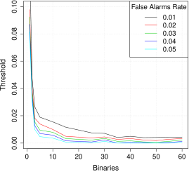
(a) FFT NA OPT, RRR-Bootstrap.

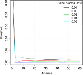
(b) FFT NA OPT, Asymptotic.

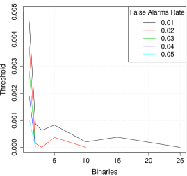
(c) Rijndael, RRR-Bootstrap.

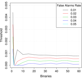
(d) Rijndael, Asymptotic.

Figure 3: False alarm rate depending on number of binaries and a threshold for performance change. Each curve is an isoquant contour, connecting the minimal combinations of thresholds and binaries that lead to no more than a given false alarm rate. A smaller rate is better, a smaller number of binaries is cheaper (better) and a smaller threshold is better. Thus, combinations to the top and right of a contour work as well, but none to the bottom and left do. Note that the shown thresholds for FFT are up to 10%, but only 0.5% for Rijndael — this means that for Rijndael, binaries do not matter.

Results for the FFT benchmark (NA OPT) are shown in Figures 3(a) and 3(b). Figure 3(a) is for the RRR-bootstrap interval, which is the default and best performing bootstrap, with replacement at all three levels. Figure 3(b) is for our asymptotic interval. These two-dimensional plots capture a three-dimensional function — the lines plotted are (isoquant) contour lines representing thresholds. For example, the red line connects all minimal combinations of binaries/thresholds that give a false alarm rate of up to 2%. In other words, the curves show how many binaries are needed to obtain less than a certain false alarm rate for a given threshold of interest. All combinations to the top and right (higher thresholds and more binaries) of the line then do as well, but none to the bottom and left do. We construct a 95% confidence interval. Hence, for large number of binaries, the false alarm rate with 0% threshold should converge to 5%. The light blue line representing the 5% false alarm rate should hence approach the $x$-axis as the number of binaries increases. The line can also disappear — if the false alarm rate gets below these 5% for a given number of binaries and remains there also for all larger numbers, it disappears in the graph at that given number of binaries.

The plots show that the false alarm rate with both methods and 0% threshold gets close to the 5% false alarm rate with an increasing number of binaries. The asymptotic method seems better than bootstrap for small numbers of binaries, say 2 to 20, but there is no practical difference for larger numbers of binaries. While being able to use less than 20 binaries in experiments would indeed be desirable, the reason for a good false alarms rate with the asymptotic method is a bad one, as we will show in Section 8.4 — the intervals are wider than they should be. On the other hand, the plots show that we could use non-zero thresholds to reduce the number of binaries needed. For a threshold of 2%, we can reach a 2% false alarm rate with only 3 binaries, using either method. Larger thresholds are even cheaper, and a threshold of 1% already helps a lot.

Technical note: the plots are based on simulated measurements for selected numbers of binaries and simulated comparisons for selected thresholds. The minimum threshold that works with a given number of binaries and a given allowed false alarm rate is found using linear interpolation. The plots also include one binary only, which corresponds to a two-level experiment in which compilation is not repeated at all (1-way classification model with the asymptotic method).

Results for all the variants of the FFT benchmark are similar. The ‘NA’ versions of FFT produce slightly fewer false alarms than the default, which could be caused by less dependence in the data, but the difference is almost negligible, and we did not attempt to verify the cause. For all FFT benchmarks, 3 binaries would be enough to obtain no more than a 5% false alarm rate with a threshold of 2%, using either method. The false alarms rate with 0% threshold converges to 5% as it should.

Results for the Rijndael benchmark are shown in Figures 3(c) and 3(d). Using either method, 2 binaries are enough to get about a 5% false alarm rate even with threshold of 0%. With the asymptotic method and the 0% threshold, the false alarm rate converges to 5% as it should. From 2 until about 30 binaries, the false alarm rate increases. With the bootstrap method, however, the false alarm rate is far too small — it is about 3% for 5 binaries and then keeps decreasing until it gets about 0.5% for 60 binaries. The reason for this is again the coverage, as we will show in Section 8.4. Other non-FFT benchmarks behaved similarly. With 0% threshold the false alarm rate converges to 5% with the asymptotic method, but to a much smaller value with the bootstrap method. The Ping benchmarks were more susceptible to non-deterministic compilation than Rijndael with the bootstrap method — more binaries were needed for the same false alarm rate. With 10 binaries and more, the bootstrap method with 0% threshold provides up to 5% false alarms, with any non-FFT benchmark. A non-zero threshold here helps as well: with 1% threshold and 2 binaries, any non-FFT benchmark with either method provides up to 1% of false alarms.

With the asymptotic method, we have seen (rare) instances of the violation of the condition in Lemma 7.7 (Section 7.3.2), and hence could not apply the method. These instances were only with 2 binaries. While this can in theory happen even for large numbers of binaries, it becomes even less likely. The bootstrap method does not have a similar problem.

Summary

The results show that choosing a non-zero threshold for comparison, even a small one (say 1%), can drastically reduce the number of binaries (and hence experimentation time) needed to get a given false alarms rate. The results also show that the asymptotic and the bootstrap methods differ in the false alarm rate even of large numbers of binaries and non-FFT benchmarks (we find the cause in Section 8.4). The results show that increasing the number of compilations does not always reduce the false alarm rate (again we find the cause in Section 8.4).

8.3.2 Ignoring Non-deterministic Compilation

Running experiments for multiple builds of the system is expensive, while Table 8.2 shows that the variation due to non-deterministic compilation is often small. Hence we quantify in more detail the impact of using only 1 binary on the false alarm rate. Results for FFT (NA OPT) and TCP Ping (OPT), with asymptotic method, are shown in Figure 4. For both benchmarks, the false alarm rate increases with the increasing number of executions. With a zero threshold, the false alarm rates are very high (nearly 60% for 100 executions). Selecting a non-zero threshold, however, helps. With TCP (OPT), we get a 5% false alarm rate with a threshold below 2% for up to 100 executions. With FFT (NA OPT), the threshold would have to be nearly 9%. We also calculated a value for one execution only, that is for a flat experiment where even non-determinism due to execution is ignored (not seen in the plots). With FFT (NA OPT) and the flat experiment, the false alarm rate with a 0% threshold is about 95%, and it is expected to be very high. A 20% threshold gets the rate down to about 9%. With TCP (OPT), the false alarm rate in a flat experiment is negligible, below 0.1% already for a 0% threshold. This is in line with Table 8.2, where the $T^{2}_{2}$ estimate (executions) is zero and $T^{2}_{3}$ (measurements) is negligible.

The results are similar for all FFT benchmarks, except that ‘NA’ versions do a bit better than non-‘NA’ (note that the variation due to non-deterministic compilation is smaller for ‘NA’ versions). All the non-FFT benchmarks show similar trends, only the false alarm rates differ corresponding to different variations (Table 8.2). We can get a 5% false alarm rate with up to 100 executions with a 1% threshold and Rijndael or HTTP benchmarks. And also with 2% threshold and TCP benchmarks.

Results for RRR bootstrap look similar with the FFT benchmarks, except that the bootstrap false alarm rates are slightly higher, and much higher for smaller numbers of executions. With the bootstrap, the rate is smallest at 5 executions (decreasing from 1 to 5, then increasing to 100). With the asymptotic method, it is increasing from 3 executions. For 2 executions, we discovered a violation of the condition in Lemma 7.7, and hence did not check the trend. For the HTTP and particularly the TCP Ping benchmarks, the RRR bootstrap false alarm rates are significantly smaller than the asymptotic ones, but the trends are the same. We will see in Section 8.4 that this is because the bootstrap method gives too wide confidence intervals for these benchmarks (their actual coverage is above 95%). For the Rijndael benchmarks, the bootstrap method provides higher rates (is worse) for small number of executions, but comparable to the asymptotic method or better for large number of executions.

Summary

It is indeed possible and desirable to measure only a single binary with benchmarks where the variability due to non-deterministic compilation is low, but a non-zero threshold and a reasonable number of executions is necessary. Oversampling by too many executions leads to increased numbers of false alarms.

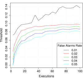
(a) FFT NA OPT, Asymptotic.

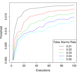
(b) TCP Ping OPT, Asymptotic.

Figure 4: False alarm rate depending on the number of executions and a threshold for performance change. These numbers represent a 2-level experiment, in which non-deterministic compilation is ignored. However, it is not ignored in the simulation, and hence an increased sample size leads to a high false alarm rate with some benchmarks. Note that the thresholds needed for TCP Ping are nearly 8$\times$ smaller than those needed for FFT.

8.3.3 Resampling with Replacement vs. Without

Our bootstrap method uses replacement at all levels of the hierarchy in the data. While this is a natural default, it was not self-evident that it would perform the best. In some cases, it has been suggested that resampling only at higher levels of the hierarchy, leaving the rest of the data intact, is better [Ren et al. (2010), Davison and Hinkley (1997)]. We therefore compare replacement at all levels (RRR) with replacement at the two higher levels (RRN) and replacement only at the highest level (RNN). We also implement a naïve solution of flat resampling with replacement (FLAT), where measurements from all executions and binaries are joined into a single set from which they are selected, ignoring the hierarchy and thus losing the original structure of the data. This also tells us what to expect in cases where a systematic source of non-determinism in the experiment has not been identified, or the hierarchy of random effects has simply been ignored and measurements were treated as if from one single execution, as is sometimes the case in current practice. The FLAT resampling, however, only corresponds to non-determinism that happens in the repeated parts of the experiment. Any source of non-determinism above (not repeated) will result in bias, instead.

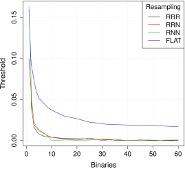
(a) FFT.

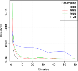
(b) TCP Ping.

Figure 5: Minimum numbers of binaries and minimum permissible thresholds for a 5% false alarm rate with different resampling techniques and the bootstrap method. A smaller number of binaries and a smaller threshold are better. Note that the thresholds needed for TCP Ping are about 10$\times$ smaller than those needed for FFT.

The results are shown in Figure 5 for the FFT benchmark (default settings) and the TCP Ping benchmark. Flat resampling is clearly the worst for both benchmarks, though for TCP it is probably still good enough, as it increases the comparison threshold needed by less than 0.5%. This is no surprise as TCP has no variation at the second level (executions) and very small variation at the third level (compilations). All of RRR, RRN, and RNN perform about the same for FFT. For TCP Ping, RRR seems somewhat better than RRN and RNN, but the corresponding difference in possible threshold is negligible. RRR ought to be better, as the other methods leave the measurements intact, while measurements are the key source of variation in this benchmark. All of these observations also apply to other benchmarks of their class (FFT, non-FFT). In the Rijndael benchmarks, though, the RRN resampling gets close to RRR. Note that in contrast to the Ping benchmarks, Rijndael’s variation is by and large due to non-deterministic execution. In summary, RRR seems as good a choice as any, does not perform worse than other methods, and we use it in all other experiments.

Note that flat resampling is particularly bad for the FFT benchmarks, which are susceptible to random effects at higher levels of the hierarchy (Table 8.2). To reliably evaluate performance changes for an FFT benchmark with a 5% false alarm rate, one would need a threshold of 2% and with it as many as 35 binaries. Note that RRR needs only 3 binaries under the same conditions, which means more than a tenfold reduction in experimentation time. On the other hand, for non-FFT benchmarks, selection of the resampling method has no practical impact, and even flat resampling is acceptable.

Summary

RRR resampling seems to be a safe choice. Replacement should be done at all the levels of the real experiment.

8.4 Coverage

The false alarms evaluation so far provides only part of the story. A method that would always give a confidence interval for performance change of say 0% $\pm$ 0.5% no matter what the data were would score best, as it would have no false alarms. Ideally, we would like to validate that the intervals our method produces are really 95% confidence intervals for the ratio of means — i.e. that they include the ratio in 95% of cases (their coverage is 95%). The consequences of improper coverage, apart from simply lack of precision in the reported uncertainty estimate, depends on how the quantified performance change is to be used. If it is to support, say, introduction of a new optimisation, which seems fairly common, the conservative default is to make the performance change seem smaller (or even zero), and hence smaller coverage is a problem, but higher coverage does not matter so much. If, on the other hand, the goal is, say, to show that a new feature has small overhead, the conservative default is to make the overhead look big, and hence higher coverage is a problem, but smaller coverage does not matter so much.

For our evaluation of coverage, we need to know what the true, but normally unknown, ratio of means is, and hence we need to assume a particular model of the data. Moreover, it has to be a simple model, so that we know the effect size based on the model parameters. Here we use a hierarchical normal model: measurements within an execution are independent identically distributed with means that also come from a normal distribution. At each level of the experiment, the distribution of the means for the lower level is normal. The grand mean ($\overline{Y}$) is then the same as the mean of the means at highest level ($\mu_{B}$ or $\mu_{n}$ in $n$-way classification, Section 7.1).

The parameters of the model are the mean $\mu=\mu_{n}$ at the highest level and the variances at all levels, $\sigma_{i}$, $1\leq i\leq n+1$. For the experiment, we choose a 5% true performance improvement, that is $\theta=^{N}\!\!\!\mu/^{O}\!\mu=0.95$. We use the same variances for both systems. Hence, the parameters of the experiment are ${}^{O}\!\mu$ and $\sigma_{i}$, $1\leq i\leq n+1$. Values of the parameters are likely to influence the resulting coverage, so we have to explore multiple selected combinations. To make the selection realistic, we feed the model with parameters estimated from the measured data, for each benchmark. We use the $S^{2}_{i}$ estimates for the variances and use three levels for all benchmarks.

Our evaluation is a statistical simulation of experiments. In each iteration we generate synthetic data for the two systems to compare — we simulate binary means, execution means, and finally individual measurements. On the simulated data of the two systems we apply our quantification methods, the (RRR) bootstrap and the asymptotic method. We report the ratio of cases in which the constructed confidence interval includes the real effect size of $\theta=0.95$. This ratio, which is our estimate of the coverage of the interval, should be 95%, as we construct 95% confidence intervals. Note that in a way, the false alarm rate experiments also provided a coverage estimate (with a 0% threshold, the false alarm rate should have been 5% with 95% intervals, because the true effect size was $\theta=1$). Here we complement those experiments with coverages for $\theta=0.95$ (a real change) and using synthetic data. Hence, in contrast to the false alarm rate experiments, the results now cannot be affected by deviations from normality, initialisation noise, lack of independence, or by heteroscedasticity.

8.4.1 Coverage in Three-level Experiment

Results of the simulation for a large number of samples at all levels (100 at each level) are shown in Figure 6. Coverages with the asymptotic method, Figure 6(b), converge to the projected 95% as the number of binaries increases. The coverages are similar for different benchmarks. They are about 99% for 3 binaries, below 98% for 10 binaries, and below 97% for 20 binaries. For 50 binaries they are 95-96%. With the bootstrap method, coverages are different for FFT and non-FFT benchmarks. For FFT benchmarks, the coverages also converge to 95% as with the asymptotic method, although they are smaller for small numbers of binaries. The non-FFT benchmarks with the bootstrap method have high coverage of about 95% for just 3 binaries and their coverage further increases up to 98-99% for 50 binaries.

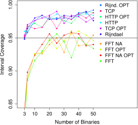
(a) RRR Bootstrap Confidence Interval.

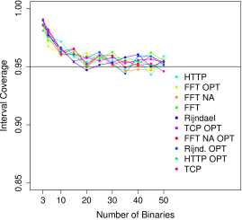
(b) Asymptotic Confidence Interval.

Figure 6: Actual coverage of a 95% confidence interval for the ratio of means, estimated in a hierarchical normal model, fed by estimated parameters from actual benchmarks.

The coverages in Figure 6 are all estimated for a large number of executions per binary. In practice, experimentation time is a precious resource. We hence looked if we could get similar coverages for smaller numbers of executions, thus saving some experimentation time. Figure 7 then shows the results for for FFT (NA OPT) and Rijndael (OPT) benchmarks. We ran the experiment for all benchmarks, but only with the asymptotic method as the bootstrap method would require too high computation costs to evaluate. In Figure 7, the coverages are colour coded. White is the projected ideal coverage of 95%. Blue denotes too high coverages, darker blue is worse (higher coverage). Red would denote smaller coverages, darker red would be worse (smaller coverage). However, in this plot, the coverage was always 95% or only slightly below, so no red colour is present. The diagonal line shows cells for the same numbers of binaries and executions.

Figure 7(a) shows that we can get close to the projected coverage of 95% with a high number of binaries, which is in line with Figure 6. Increasing the number of executions per binary does not seem to impact the coverage. Figure 7(b) shows that the Rijndael benchmark performs similarly. The other benchmarks do as well. This suggests that the repetition count at the highest level is most important for coverage. Note that we have shown in Section 7.4 that the repetition at some lower level can, however, be important for getting most precise results (narrowest intervals) within given experimentation time.

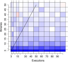
(a) FFT NA OPT (from 94.8% to 98.9%).

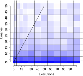
(b) Rijndael OPT (from 95% to 98.9%).

Figure 7: Actual coverage of a 95% asymptotic confidence interval for the ratio of means, estimated in a hierarchical normal model, fed by estimated parameters from actual benchmarks. White is the 95% coverage. Red is smaller coverage (darker is worse-smaller), blue is higher coverage (darker is worse-higher). Overall, white is ideal, darker is worse than lighter, and red is usually worse than blue. The diagonal line denotes the same numbers of binaries and executions. If printed in greyscale, note that the plots are almost completely blue — the coverage is only rarely below 95%, and if so, only slightly.

We also explored coverages with the asymptotic method, but using only the normal approximation instead (“normal-asymptotic”) of the $t$-distribution (“asymptotic”). See Section 7.3.2 for more details. With the normal-asymptotic method, the coverages are too small for small number of binaries (around 88% for 3 binaries), but converge to the projected 95% as the number of binaries increases. They get above 90% for 5 binaries and above 94% for 15 binaries. Similarly to the asymptotic method, it is the number of binaries that impacts (improves) the coverage, not the number of executions. We also ran the false alarms experiments with the normal-asymptotic method. The false alarm rate with 0% threshold converged to 5% with all benchmarks. As in practice a too-high coverage is often worse than too-low coverage, it makes sense to use the asymptotic method ($t$-distribution) even in cases when the normality assumptions cannot be made.

Summary

With the asymptotic method, the coverage is too large for small numbers of binaries, but converges to the projected number as the number of binaries increases. With the bootstrap method, the coverage of FFT benchmarks is too low for small numbers of binaries, but then converges to the projected number. The coverage of non-FFT benchmarks with the bootstrap is always too large. With the asymptotic method but only the normal approximations, the coverages also converge to the projected number (all benchmarks), but are too small for small number of binaries. In most cases, the asymptotic method would be the best choice. The number of executions does not have an impact on the coverage.

8.4.2 Ignoring Non-deterministic Compilation

With the non-FFT benchmarks, the performance variation due to non-deterministic compilation is very small (1%, Table 8.2 below). In practice, one would probably choose not to repeat compilations with these benchmarks, but rather select an appropriate comparison threshold. In another simulation, we look at what the true coverage would be if we choose to do this. The experiment we simulate ignores variation due to non-deterministic compilation, but the simulation does not. Figure 8 shows the results, for the asymptotic method and varying numbers of executions. The coverage decreases with increasing number of executions. This is expected, because as the intervals get narrower, they are more likely to miss the true mean that takes many different binaries into account. This reduction is first good with the asymptotic method (all benchmarks) and the bootstrap method (non-FFT benchmarks), because it corrects for the over-coverage of these methods. But, the coverage soon gets unacceptably low and not only so with the FFT benchmarks, which are prone to non-deterministic compilation to a high degree. The coverage also gets too low with an unduly large number of binaries with the non-FFT benchmarks where this impact is very small.

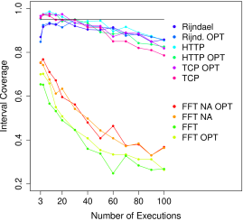
(a) RRR Bootstrap Confidence Interval.

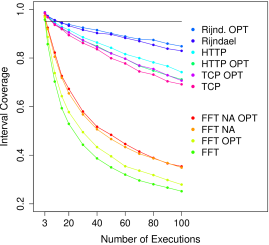
(b) Asymptotic Confidence Interval.

Figure 8: Actual coverage of a 95% confidence interval for the ratio of means, estimated in a hierarchical normal model. In contrast to Figure 6, this plot simulates a 2-level only experiment (a scenario in which the experimenter would choose to ignore uncertainty due to compilation). Closer to 0.95 is better.

We also looked at the trade-offs between the repetition counts for measurements per execution and executions per binary, with respect to coverage. We ran the experiments with the asymptotic method only. Figure 9 shows the results for the FFT NA and HTTP Ping OPT benchmarks. With the FFT NA benchmark, the number of measurements per execution do not seem to make a difference. The too-high coverage gets first better and then too small, as the number of executions increases, as in Figure 8(b). Other FFT benchmarks behave similarly. With the HTTP Ping OPT benchmark, the number of measurements per execution matters once the number of executions is high. Increasing the number of measurements makes the coverage worse, no matter from how many executions these measurements are. Other Ping benchmarks behave similarly, except that the coverages are higher than with FFT. The Rijndael benchmarks lie in between — increasing the number of measurements per execution makes the coverage worse, but perhaps not as strongly as with the Ping benchmarks. The differences between benchmarks can be explained with the variations at different levels (Table 8.2). In this experiment, anything that makes the interval narrower makes also the coverage worse. With FFT benchmarks, variation due to non-deterministic execution is much larger than that due to non-deterministic measurement, and hence the coverage decreases more with increased executions. With the other benchmarks and particularly the Ping benchmarks, variation due to execution is far smaller than that due to measurement, and hence the number of executions is not important in reducing the coverage.

Summary

When non-deterministic compilation has minimal impact on variability in performance, it makes sense to use only one binary. However, over-sampling (too many executions and/or measurements, depending on the benchmark) can inflate the influence of ignored variability due to compilation and result in a too low coverage.

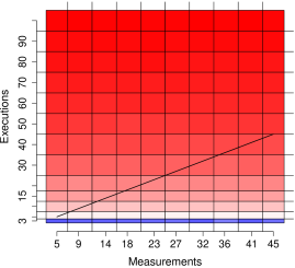
(a) FFT NA (from 34% to 98%).

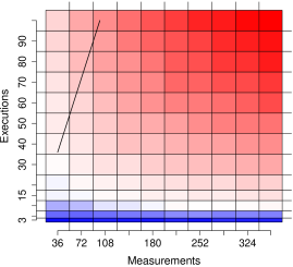
(b) HTTP OPT (from 72% to 99%)

Figure 9: Actual coverage of a 95% asymptotic confidence interval for the ratio of means, estimated in a hierarchical normal model. In contrast to Figure 7, this plot simulates a 2-level only experiment (a scenario in which the experimenter would choose to ignore uncertainty due to compilation). If printed in greyscale, note that the plots have a blue line of cells at about 3 executions, while all cells above are red. The tone of the red colour does not match in the two plots — the coverage of FFT is far worse.

8.5 Dimensioning the Experiments

We compare the results precision that would be obtained with our method against the default single-level method.

Let us first focus on the FFT benchmark (descriptions of the benchmarks were given in Section 8.1) and let us assume we have a window of 6 hours for our experiments. From Table 8.2 we see that the benchmark has high variation at all three levels, including compilation, and hence multiple binaries have to be measured.

The usual one-level approach would execute each binary once, obtaining one measurement (after warmup). One execution with one measurement (and 19 warm-up measurements) takes about 5 seconds. Compilation takes about 20 minutes (1200 seconds), so we can take about $6*3600/1205=17$ samples within our 6 hours. We would calculate the sample mean from these 17 samples and provide an asymptotic confidence interval based on t-test like e.g. in [Lilja (2000), Jain (1991), Georges et al. (2007)]. The half-width of such 95% interval would be about 4.7% of the mean with the FFT benchmark ($\pm 4.7\%$), as we can derive from Equation 10 on page 10 and the definition of the t-test:

$$\left(1/\overline{Y}\right)t_{1-\frac{\alpha}{2}}\sqrt{var(\overline{Y})}=\left(1/\overline{Y}\right)t_{1-\frac{\alpha}{2}}\sqrt{\frac{\sigma_{3}^{2}+\sigma_{2}^{2}+\sigma_{1}^{2}}{17}}$$

We substitute the sample mean and the unbiased estimates $T_{i}^{2}$ of variances $\sigma_{i}^{2}$.

With the method we propose in this work, we dimension the experiment using Equation 13 on page 13. We would collect $n_{1}$ measurements from each execution and run each binary $n_{2}$ times, where:

$$n_{1}=\left\lceil\sqrt{c_{1}\frac{\sigma^{2}_{1}}{\sigma^{2}_{2}}}\right\rceil\quad\textrm{and}\quad n_{2}=\left\lceil\sqrt{\frac{c_{2}}{c_{1}}\frac{\sigma^{2}_{2}}{\sigma^{2}_{3}}}\right\rceil\\$$

The costs are $c_{1}=19$ (19 warmup measurements) and $c_{2}=5343$ (number of measurements that could roughly be done in 20 minutes, the time needed for compilation). Substituting the unbiased estimates $T_{i}^{2}$ of variances $\sigma_{i}^{2}$, we get $n_{1}=4$ and $n_{2}=28$. One execution will take within 6 seconds (4 measurements and warmup) and all executions of one binary will take about 150 seconds, and so within 6 hours we can build and measure $\left\lfloor 6*3600/1350\right\rfloor=16$ binaries, obtaining 1792 samples. Using Equation 11 on page 11 we would calculate a 95% confidence interval for the mean, half-width of which would about 2.3% of the mean ($\pm 2.3\%$ instead of the $\pm 4.7\%$ with the single-level method).

Interval half-widths for all benchmarks and for experimentation windows of 3,6, and 9 hours are shown in Table 8.5. Our method would use the 3-level model for all FFT and Rijndael benchmarks. With HTTP and TCP benchmarks, it would only execute each binary once, but collecting multiple measurements. It would not repeat executions because variation due to execution in those benchmarks is small (and the $T_{2}^{2}$ estimate turns negative). Our method is always better than the default method (and by design it should never be worse). The benefits are particularly big when the variation due to non-deterministic compilation is far below variations at lower levels (see Table 8.2).

Note that when running multiple benchmarks on different versions of the same managed runtime, one can re-use the binaries of the runtime. Even in this case there would be a balance between spending time on compiling or on running existing binaries, but the optimisation procedure would need to be extended and will require a summarization technique over different benchmarks.

Result Precision with Our Method and the Default Method 95% Confidence Interval Half-width (smaller is better) 3 hours exp. [our/default] 6 hours exp. [our/default] 9 hours exp. [our/default] FFT NA OPT 3. 3 % / 7. 5% 2. 0 % / 4. 6% 1. 5 % / 3. 6% FFT NA 3. 2 % / 7. 1% 1. 9 % / 4. 4% 1. 5 % / 3. 4% FFT OPT 4. 3 % / 8. 6% 2. 5 % / 5. 3% 2. 0 % / 4. 1% FFT 3. 6 % / 7. 6% 2. 3 % / 4. 7% 1. 8 % / 3. 7% HTTP OPT 0. 5 % / 18. 8% 0. 3 % / 11. 5% 0. 3 % / 9. 1% HTTP 0. 4 % / 18. 0% 0. 3 % / 11. 1% 0. 2 % / 8. 7% Rijndael OPT 1. 3 % / 8. 3% 0. 2 % / 5. 1% 0. 1 % / 4. 0% Rijndael 0. 6 % / 8. 1% 0. 2 % / 5. 0% 0. 2 % / 3. 9% TCP OPT 1. 3 % / 34. 9% 0. 8 % / 21. 5% 0. 6 % / 16. 9% TCP 1. 3 % / 32. 2% 0. 8 % / 19. 8% 0. 6 % / 15. 5% Source:Relative half-widths of 95% confidence interval for the mean (relative to the grand mean) with our method and the default single-level method. Smaller is better. Shown for 3, 6, and 9 hours time windows for experimentation. Our method repeats executions and/or measurements where it is beneficial to improve result precision, but the default method can only use one execution and measurement from a binary. With FFT and Rijndael benchmarks, our method uses both multiple executions per binary and multiple measurements per execution. With TCP and HTTP, it uses a single execution per binary but multiple measurements, as it leads to better precision. Our method is always better, and particularly more so when the variation due to compilation is smaller than variations due to effects at lower levels.

8.6 Summary of Evaluation

Our evaluation has demonstrated that both the bootstrap and the asymptotic method work reasonably well. For the bootstrap, resampling with replacement at all levels (RRR) is a safe choice. For the asymptotic method, using the $t$-distribution even when normality assumptions cannot be made seems a safe choice. It is particularly more conservative (produces wider intervals) than relying just on asymptotic normality. The asymptotic method in theory may fail to provide a result when the sample mean of the “old” system appears not significantly different from zero. We have seen it happen, but only for 2 or 3 binaries/executions, never for larger sample sizes. The coverages with the asymptotic method converge to the projected value. With the bootstrap method, this is however not the case with all the benchmarks. The non-FFT benchmarks, which means those of our benchmarks with high variation due to non-deterministic compilation, always have too high coverages. What has not been shown in the analysis is that the bootstrap method is easier to implement, and perhaps to understand, than the asymptotic method, but takes more computation time. The computation time, though, should not be a problem in a regular application of the method, when only a few intervals need to be constructed.

We demonstrated that choosing a non-zero threshold for comparisons simplifies the quantification considerably — it reduces the necessary experimentation time (total number of samples, expensive repetitions of compilation and execution) and/or the false alarm rate. It may even completely eliminate the need for repetition at the highest level (i.e. compilations) when the variation caused by non-determinism at that level is small. Repeating compilations was necessary with the FFT benchmarks. With the other benchmarks, using a single binary with a well chosen threshold would provide the same results and indeed reduce experimentation time. The Ping benchmarks would not need repetition of executions, either. Hence, even with the same system to test (in our case Mono), one can expect different benchmarks to have very different needs for statistical modeling. Selection of good repetition counts is important — too low and too high counts lead to poor coverage and a high false alarm rate, but selecting a sensible (non-zero) threshold reduces this problem in practice.

Note that the necessity of repeating compilation of FFT benchmarks in Mono is by itself an important observation. FFT benchmarks are (still) used as we have seen in our survey of the “2011” papers mentioned previously (15 of all 122 papers measured also FFT). In one case, the evaluation with FFT even used the Mono platform. As compilation is expensive one needs to balance carefully whether to spend time on more executions of existing binaries or to produce more binaries. A similar tradeof is between running more measurements of the same execution, or investing into starting (and warming up) a new execution. These tradeoffs are different for each benchmark, and out method allows to find the optimum numbers.

9 Conclusion

Empirical evaluations in computing, particularly in programming languages and systems research, are dominated by quantification of performance change measured by the ratio of execution times. Regrettably, we find that evaluations reported even at premier venues commonly fail to report uncertainty in measurements or to cater for non-determinism from various sources.

In this work we attack both problems — we have created a statistical model that captures such non-determinism and we show how to construct a confidence interval for the ratio of means within the model. Our model is based on general assumptions and caters for random factors that influence performance and factors that the experimenter intentionally randomizes to reduce bias. We evaluate our method experimentally using statistical simulation on a set of benchmarks.

The best method for quantification of performance change recommended in the field to date is based on a visual test for overlap of confidence intervals and only provides a binary answer as to whether the difference seen is unlikely to be by pure chance. Our method can provide the same answer, if needed. However, such an answer is usually not needed — what is needed is an uncertainty estimate for the ratio of means, and our method provides that as well.

We have learned a number of lessons along the way. Introductory statistical textbooks offer insufficient guidance to advance evaluation practice in computer systems, because these are not updated fast enough nor with computer systems in mind. Books specializing in computer systems performance evaluation explain statistical methods in the context of computer science, but still only include mostly introductory statistics, which leads to recommendations of limited applicability. It may be that lack of applicability also contributes to the poor adoption of their recommendations, though it may also be that there is simply not enough pressure to do better evaluations. To move forward, we need to consult methods in the original statistical publications, and we sometimes need to adapt them to our field. As a part of that, we need to advance our knowledge of the various factors in computer systems that influence performance. The work we present here is based on both of these activities.

While our method is better than the best recommended one, and even more so than current practice, it does not solve all problems. More work needs to be done to incorporate fixed effects, that is effects of factors such as hardware platform or operating system, which only have a small set of values controlled by the user and experimenter. This should be doable, and fixed effects have been addressed even in books on computer systems performance evaluation. There is a need for further work on rigorous summarization over different benchmarks. Apart from better statistics, we need better benchmarks, benchmarks better analysed, and we could and should improve the experimentation practice in our field by bringing more of the scientific method used in “real” science, particularly physics and natural sciences — thorough reports, archival of experimental artifacts, repeatability and, most importantly, reproducibility demonstrated through independent reproduction studies.

References

- Alameldeen and Wood (2003) Alameldeen, A. R. and Wood, D. A. 2003. Variability in architectural simulations of multi-threaded workloads. In Proceedings of the 9th Annual International Symposium on High-Performance Computer Architecture (HPCA). IEEE, Anaheim, CA.
- American Psychological Association (2001) American Psychological Association. 2001. Publication Manual of the American Psychological Association (5th edition).
- Basu and DasGupta (1995) Basu, S. and DasGupta, A. 1995. Robustness of standard confidence intervals for location parameters under departure from normality. Annals of Statistics 23, 4, 1433–1442.
- Beyene and Moineddin (2005) Beyene, J. and Moineddin, R. 2005. Methods for confidence interval estimation of a ratio parameter with application to location quotients. BMC Medical Research Methodology 5, 1.
- Bland and Altman (2000) Bland, J. M. and Altman, D. G. 2000. The odds ratio. BMJ 320, 7247.
- Boyer (2008) Boyer, B. 2008. Robust java benchmarking, part 2: Statistics and solutions. https://www.ibm.com/developerworks/java/library/j-benchmark2/.
- Charles E. McCulloch (2008) Charles E. McCulloch, Shayle R. Searle, J. M. N. 2008. Generalized, Linear, and Mixed Models. Wiley.
- Cochran (1977) Cochran, W. G. 1977. Sampling Techniques: Third Edition. Wiley.
- Coe (2002) Coe, R. 2002. It’s the effect size, stupid: What effect size is and why it is important. In Annual Conference of the British Educational Research Association (BERA).
-
Cohen (1994)
Cohen, J. 1994.
The Earth is round (p
<.05). American Psychologist, 997–1003. - Curtsinger and Berger (2012) Curtsinger, C. and Berger, E. D. 2012. Stabilizer: Enabling statistically rigorous performance evaluation. Tech. rep., University of Massachusetts, Amherst.
- Davison and Hinkley (1997) Davison, A. C. and Hinkley, D. V. 1997. Bootstrap Methods and Their Applications. Cambridge University Press.
- Dilba et al. (2007) Dilba, G., Schaarschmidt, F., and Hothorn, L. A. 2007. Inferences for ratios of normal means. R News 7, 1.
- Dunleavy et al. (2006) Dunleavy, E. M., Barr, C. D., Glenn, D. M., and Miller, K. R. 2006. Effect size reporting in applied psychology: How are we doing? The Industrial-Organizational Psychologist 43, 4.
- Erceg-Hurn and Mirosevich (2008) Erceg-Hurn, D. M. and Mirosevich, V. M. 2008. Modern robust statistical methods: An easy way to maximize the accuracy and power of your research. American Psychologist 63, 7, 591–601.
- Fidler and Cumming (2007) Fidler, F. and Cumming, G. 2007. Psychology in the Schools 44, 5.
- Fieller (1954) Fieller, E. C. 1954. Some problems in interval estimation. Journal of the Royal Statistical Society, 175–185.
- Georges (2008) Georges, A. 2008. Three pitfalls in java performance evaluation. Ph.D. thesis, Ghent University.
- Georges et al. (2007) Georges, A., Buytaert, D., and Eeckhout, L. 2007. Statistically rigorous Java performance evaluation. In Proceedings of the 22nd annual ACM SIGPLAN conference on Object-Oriented Programming Systems, Languages and Applications (OOPSLA). ACM.
- Georges et al. (2008) Georges, A., Eeckhout, L., and Buytaert, D. 2008. Java performance evaluation through rigorous replay compilation. In Proceedings of the 23rd ACM SIGPLAN conference on Object-Oriented Programming Systems, Languages and Applications (OOPSLA). ACM.
- Gu et al. (2004) Gu, D., Verbrugge, C., and Gagnon, E. 2004. Code layout as a source of noise in JVM performance. In Component And Middleware Performance Workshop, OOPSLA 2004.
- Hill and Thompson (2005) Hill, C. and Thompson, B. 2005. Computing and interpreting effect sizes. In Higher Education: Handbook of Theory and Research. Vol. 19. Springer, 175–196.
- Jain (1991) Jain, R. 1991. The Art of Computer Systems Performance Analysis. Wiley.
- Kalibera et al. (2005) Kalibera, T., Bulej, L., and Tuma, P. 2005. Automated detection of performance regressions: The Mono experience. In Proceedings of the 13th International Symposium on Modeling, Analysis, and Simulation of Computer and Telecommunication Systems (MASCOTS). IEEE.
- Kalibera and Tuma (2006) Kalibera, T. and Tuma, P. 2006. Precise regression benchmarking with random effects: Improving Mono benchmark results. In Proceedings of Third European Performance Engineering Workshop (EPEW). LNCS Series, vol. 4054. Springer.
- Kirkup (1994) Kirkup, L. 1994. Experimental Methods: An Introduction to the Analysis and Presentation of Data. Wiley.
- Lilja (2000) Lilja, D. J. 2000. Measuring Computer Performance: A Practitioner’s Guide. Cambridge University Press.
- Luo and John (2004) Luo, Y. and John, L. K. 2004. Efficiently evaluating speedup using sampled processor simulation. IEEE Comput. Archit. Lett. 3, 1.
- Maxwell and Delaney (2004) Maxwell, S. E. and Delaney, H. D. 2004. Designing experiments and analyzing data: a model comparison perspective. Routledge.
- Mytkowicz et al. (2009) Mytkowicz, T., Diwan, A., Hauswirth, M., and Sweeney, P. F. 2009. Producing wrong data without doing anything obviously wrong! In Proceeding of the 14th international conference on Architectural Support for Programming Languages and Operating Systems (ASPLOS). ACM.
- Nakagawa and Cuthill (2007) Nakagawa, S. and Cuthill, I. C. 2007. Effect size, confidence interval and statistical significance: a practical guide for biologists. Biological Reviews 82, 4, 591–605.
- Novell, Inc. (2011) Novell, Inc. 2011. The Mono Project. http://www.mono-project.com.
- Oakes (1986) Oakes, M. 1986. Statistical Inference: A Commentary for the Social and Behavioural Sciences. Wiley.
- O’Sullivan (2009) O’Sullivan, B. 2009. The Criterion package. http://hackage.haskell.org/package/criterion.
- Payton et al. (2003) Payton, M. E., Greenstone, M. H., and Schenker, N. 2003. Overlapping confidence intervals or standard error intervals: What do they mean in terms of statistical significance? Journal of Insect Science 3, 1996.
- Pozo and Miller (2005) Pozo, R. and Miller, B. 2005. SciMark 2.0 benchmark. http://math.nist.gov/scimark2/.
- Rasch and Guiard (2004) Rasch, D. and Guiard, V. 2004. The robustness of parametric statistical methods. Psychology Science 46, 2, 175–208.
- Re and Vogels (2011) Re, C. and Vogels, W. 2011. SciMark – C#. http://code.google.com/p/scimark-csharp/.
- Ren et al. (2010) Ren, S., Lai, H., Tong, W., Aminzadeh, M., Hou, X., and Lai, S. 2010. Nonparametric bootstrapping for hierarchical data. Journal of Applied Statistics 37, 9, 1487–1498.
- Royall (1986) Royall, R. M. 1986. The effect of sample size on the meaning of significance tests. American Statistician 40, 4.
- Schaarschmidt (2007) Schaarschmidt, F. 2007. Confidence intervals for the ratio of means of two normal distributed populations in the presence of heteroscedasticity. Reports of the Institute of Biostatistics 17, Leibniz University of Hanover.
- Schenker and Gentleman (2001) Schenker, N. and Gentleman, J. F. 2001. On judging the significance of differences by examining the overlap between confidence intervals. The American Statistician 55, 3, 182–186.
- Searle et al. (1992) Searle, S. R., Casella, G., and McCulloch, C. E. 1992. Variance Components. Wiley.
- Singer et al. (2011) Singer, J., Kovoor, G., Brown, G., and Lujan, M. 2011. Garbage collection auto-tuning for Java map-reduce on multi-cores. In Proceedings of the International Symposium on Memory management (ISMM). ACM.
- Steele (2001) Steele, J. M. 2001. Stochastic calculus and financial applications. Springer.
- Taylor and Kuyatt (1994) Taylor, B. N. and Kuyatt, C. E. 1994. Guidelines for evaluating and expressing the uncertainty of NIST measurement results. Technical Note 1297, National Institute of Standards and Technology.
- von Luxburg and Franz (2009) von Luxburg, U. and Franz, V. 2009. A geometric approach to confidence sets for ratios: Fieller’s theorem, generalizations, and bootstrap. Statistica Sinica 19, 3.
- Wasserman (2004) Wasserman, L. 2004. All of Statistics: A Concise Course in Statistical Inference. Springer.
- Wilson (1952) Wilson, E. B. 1952. An Introduction to Scientific Research. McGraw Hill.