Refined Cauchy identity for spin Hall–Littlewood symmetric rational functions

Abstract.

Fully inhomogeneous spin Hall–Littlewood symmetric rational functions $\mathsf{F}_{\lambda}$ arise in the context of $\mathfrak{sl}(2)$ higher spin six vertex models, and are multiparameter deformations of the classical Hall–Littlewood symmetric polynomials. We obtain a refined Cauchy identity expressing a weighted sum of the product of two $\mathsf{F}_{\lambda}$’s as a determinant. The determinant is of Izergin–Korepin type: it is the partition function of the six vertex model with suitably decorated domain wall boundary conditions. The proof of equality of two partition functions is based on the Yang–Baxter equation.

We rewrite our Izergin–Korepin type determinant in a different form which includes one of the sets of variables in a completely symmetric way. This determinantal identity might be of independent interest, and also allows to directly link the spin Hall–Littlewood rational functions with (the Hall–Littlewood particular case of) the interpolation Macdonald polynomials. In a different direction, a Schur expansion of our Izergin–Korepin type determinant yields a deformation of Schur symmetric polynomials.

In the spin-$\frac{1}{2}$ specialization, our refined Cauchy identity leads to a summation identity for eigenfunctions of the ASEP (Asymmetric Simple Exclusion Process), a celebrated stochastic interacting particle system in the Kardar–Parisi–Zhang universality class. This produces explicit integral formulas for certain multitime probabilities in ASEP.

1. Introduction

1.1. Background

This paper deals with summation identities for spin Hall–Littlewood symmetric rational functions. These functions appeared in [Bor17], [BP18] as partition functions (with boundary conditions of a rather general form) of square lattice vertex models possessing Yang–Baxter integrability which is traced to the quantum group $U_{q}(\widehat{\mathfrak{sl}_{2}})$.

The spin Hall–Littlewood functions may also be identified with Bethe Ansatz eigenfunctions of the higher spin six vertex model on $\mathbb{Z}$, cf. [KBI93, Ch. VII]. They also arise as eigenfunctions of certain stochastic particle systems [Pov13], [BCPS15], [CP16]. In [Bor17], [BP18] and subsequent works the spin Hall–Littlewood functions and their relatives are treated from the point of view of the theory of symmetric functions. A classical reference on symmetric functions in the book [Mac95] where Schur, Hall–Littlewood, and Macdonald symmetric polynomials and symmetric functions (= property understood symmetric polynomials in infinitely many variables) are developed.

One of the most important features common for many families of symmetric polynomials is a Cauchy type summation identity. For example, the Hall–Littlewood polynomials ([Mac95, Ch. III]; we also briefly recall them in Section 5 below) satisfy the following Cauchy type identity:

$$\sum_{\lambda_{1}\geq\lambda_{2}\geq\ldots\geq\lambda_{N}\geq 0}P_{\lambda}^{HL}(u_{1},\ldots,u_{N};\mathfrak{t})\,Q_{\lambda}^{HL}(v_{1},\ldots,v_{N};\mathfrak{t})=\prod_{i,j=1}^{N}\frac{1-\mathfrak{t}u_{i}v_{j}}{1-u_{i}v_{j}},$$ (1.1)

where the sum is over ordered $N$-tuples of integers $\lambda$. In [Bor17], [BP18] similar Cauchy type summation identities were proven for the spin Hall–Littlewood symmetric functions. The proofs are based on the Yang–Baxter equation for the higher spin six vertex model. Namely, both sides are identified as certain partition functions which are equal thanks to a sequence of elementary Yang–Baxter steps. The product in the right-hand side comes from the fact that the corresponding partition function has only one nontrivial configuration.

We are interested in refinements of Cauchy type identities like (1.1) which are obtained by inserting a new factor (depending on $\lambda$) into each term in the sum over $\lambda$ in the left-hand side. This complicates the right-hand side: instead of a relatively simple product it becomes a determinant.

Refinements of Cauchy type identities for various symmetric functions appeared since [KN99], [War08], see also [BW16], [BWZJ15]. In [WZJ16], a novel method for proving a number of refined Cauchy (and also Littlewood) type identities was introduced based on the Yang–Baxter equation. Namely, the determinant in the right-hand side of a refined identity arises as the partition function of the six-vertex model with domain wall boundary conditions (or a suitable modification thereof). The domain wall six vertex partition function is given by the celebrated Izergin–Korepin determinant [Ize87], [KBI93, Ch. VII.10]. The particular determinantal answer for each refined identity is uniquely identified with the help of Lagrange interpolation.

Remark 1.1.

After completing this manuscript, another refined summation identity for the spin Hall–Littlewood functions — a Littlewood-type identity — was proven in [Gav21]. See also [CD21] for probabilistic applications of Littlewood-type identities for the spin Hall–Littlewood functions.

1.2. Refined Cauchy identity for spin Hall–Littlewood functions

Our first main result is a lifting of the refined Cauchy identity for Hall–Littlewood polynomials to the spin Hall–Littlewood level. Namely, we consider the fully inhomogeneous spin Hall–Littlewood symmetric rational functions introduced in [BP18] which have the following explicit symmetrization form:

$$\begin{split}\mathsf{F}_{\lambda}(u_{1},\ldots,u_{N})&=\sum_{\sigma\in S_{N}}\sigma\Biggl{(}\prod_{1\leq i<j\leq N}\frac{u_{i}-qu_{j}}{u_{i}-u_{j}}\,\prod_{i=1}^{N}\biggl{(}\frac{1-q}{1-s_{\lambda_{i}}\xi_{\lambda_{i}}u_{i}}\prod_{j=0}^{\lambda_{i}-1}\frac{\xi_{j}u_{i}-s_{j}}{1-\xi_{j}s_{j}u_{i}}\biggr{)}\Biggr{)},\end{split}$$

where $\lambda=(\lambda_{1}\geq\ldots\geq\lambda_{N}\geq 0)$. Here $\sigma\in S_{N}$ acts by permuting the $u_{i}$’s and not the $\lambda_{i}$’s. We employ the same convention about permutation action in all symmetrization formulas throughout the text. The function $\mathsf{F}_{\lambda}$ depends on the “quantum parameter” $q$, the variables $u_{j}$, and the inhomogeneities $\xi_{x}$ and $s_{x}$, where $x\in\mathbb{Z}_{\geq 0}$. These parameters are assumed to be generic complex numbers. When required, for certain statements (like in Theorem 1.2 below) we impose additional conditions on the parameters. If $s_{x}=0$ and $\xi_{x}=1$ for all $x$, then the functions $\mathsf{F}_{\lambda}$ reduce to the usual Hall–Littlewood symmetric polynomials.

To formulate the result we need more notation. Let $m_{0}(\lambda)$ is the number of parts in $\lambda$ equal to zero (so that $\lambda_{N-m_{0}(\lambda)}>0$ and $\lambda_{N-m_{0}(\lambda)+1}=0$), and $(a;q)_{k}=(1-a)(1-aq)\ldots(1-aq^{k-1})$ be the $q$-Pochhammer symbol. We also employ dual spin Hall–Littlewood functions $\mathsf{F}_{\lambda}^{*}$ which are given by a symmetrization expression similarly to $\mathsf{F}_{\lambda}$, see formulas (2.3), (2.6) in the text.

Theorem 1.2 (Refined Cauchy identity for spin Hall–Littlewood functions).

For any $\gamma\neq 0$ and provided that $u_{i},v_{j},s_{x},\xi_{x}$ satisfy certain conditions so that the series in the left-hand side converges (see (2.8) in the text), we have

$$\sum_{\lambda=(\lambda_{1}\geq\lambda_{2}\geq\ldots\geq\lambda_{N}\geq 0)}\frac{(\gamma q;q)_{m_{0}(\lambda)}(\gamma^{-1}s_{0}^{2};q)_{m_{0}(\lambda)}}{(q;q)_{m_{0}(\lambda)}(s_{0}^{2};q)_{m_{0}(\lambda)}}\,\mathsf{F}_{\lambda}(u_{1},\ldots,u_{N})\,\mathsf{F}^{*}_{\lambda}(v_{1},\ldots,v_{N})$$

$$\hskip 30.0pt=\prod_{j=1}^{N}\frac{1}{(1-s_{0}\xi_{0}u_{j})(1-\xi_{0}^{-1}s_{0}v_{j})}\,\frac{\prod_{i,j=1}^{N}(1-qu_{i}v_{j})}{\prod_{1\leq i<j\leq N}(u_{i}-u_{j})(v_{i}-v_{j})}$$ (1.2)

$$\hskip 56.0pt\times\det\left[\frac{(1-\gamma)(q-\gamma^{-1}s_{0}^{2})(1-u_{i}v_{j})+(1-q)(1-\xi_{0}s_{0}u_{i})(1-\xi_{0}^{-1}s_{0}v_{j})}{(1-u_{i}v_{j})(1-qu_{i}v_{j})}\right]_{i,j=1}^{N}.$$

Observe that a priori the left-hand side of (1.2) should depend on the parameters $s_{x},\xi_{x}$ for all $x\in\mathbb{Z}_{\geq 0}$. However, it turns out that the dependence on all of them except $(s_{0},\xi_{0})$ is artificial and disappears after summing over $\lambda$.

We prove Theorem 1.2 in Section 3 with the help of the Yang–Baxter equation. The Izergin–Korepin type determinant in the right-hand side of (1.2) comes from the partition function of the six vertex model with suitably decorated domain wall boundary conditions, and is uniquely identified with the help of Lagrange interpolation. That is, we formulate a number of properties which follows from the description of the six vertex partition function, and check that the determinant satisfies these properties (uniqueness is guaranteed by Lagrange interpolation). This approach to proving the refined identity is essentially parallel to [WZJ16]. However, one of the steps in identifying the Izergin–Korepin type determinant turns out to be more involved and requires to compute a nontrivial auxiliary determinant which evaluates in a product form (see Lemma 3.9 in the text).

1.3. Determinantal identity

Our next result is an alternative determinantal expression for the right-hand side of the refined Cauchy identity (1.2). Namely, we observe that the (suitably normalized) determinant in the right-hand side of (1.2) is a skew-symmetric polynomial in $v_{1},\ldots,v_{N}$. As such, it should be divisible by the product $\prod_{i<j}(v_{i}-v_{j})$ in the denominator. Remarkably, the ratio admits a nice determinantal form which includes all the variables $v_{1},\ldots,v_{N}$ in a manifestly symmetric way:

Theorem 1.3.

The following identity of $N\times N$ determinants holds:

$$\begin{split}&\frac{\prod_{i,j=1}^{N}(1-qu_{i}v_{j})}{\prod_{1\leq i<j\leq N}(v_{i}-v_{j})}\,\det\left[\frac{(1-\gamma)(q-\gamma^{-1}s_{0}^{2})(1-u_{i}v_{j})+(1-q)(1-\xi_{0}s_{0}u_{i})(1-\xi_{0}^{-1}s_{0}v_{j})}{(1-u_{i}v_{j})(1-qu_{i}v_{j})}\right]_{i,j=1}^{N}\\ &\hskip 20.0pt=\det\Biggl{[}u_{j}^{N-i-1}\biggl{\{}\left(1-s_{0}\xi_{0}u_{j}\right)\left(u_{j}-\frac{s_{0}}{\xi_{0}}\right)\prod_{l=1}^{N}\frac{1-qu_{j}v_{l}}{1-u_{j}v_{l}}\\ &\hskip 200.0pt-\gamma^{-1}q^{N-i}(\gamma-s_{0}\xi_{0}u_{j})\left(\gamma qu_{j}-\frac{s_{0}}{\xi_{0}}\right)\biggr{\}}\Biggr{]}_{i,j=1}^{N}.\end{split}$$ (1.3)

We prove Theorem 1.3 in Section 4 by checking that the (suitably normalized) right-hand side of (1.3) satisfies properties which identify the answer by Lagrange interpolation. This involves computing another nontrivial auxiliary determinant. This determinant is related to the tridiagonal matrix of three-term relation coefficients for the $q$-Krawtchouk orthogonal polynomials [KS96, Section 3.15]. Using this connection, we are able to evaluate the determinant in a product form (see Lemma 4.4 in the text).

1.4. Relation to interpolation Hall–Littlewood polynomials

The determinantal identity of Theorem 1.3 generalizes the one from [Cue18, Section 4.5]; the latter is recovered by setting $s_{0}=0$ in (1.3).

The paper [Cue18] in particular deals with the Hall–Littlewood particular case $F_{\lambda}^{HL}$ of interpolation Macdonald symmetric polynomials [Kno97], [Oko97], [Sah96], and derives a refined Cauchy identity for them. In that identity, the determinant in the right-hand side is like the one in the right-hand side of (1.3). Combining this with the Izergin–Korepin type determinant from [WZJ16] leads to a determinantal identity given in [Cue18, Section 4.5].

This connection between determinants suggests a direct limit transition from the fully inhomogeneous spin Hall–Littlewood symmetric rational functions $\mathsf{F}_{\lambda}$ to the inhomogeneous Hall–Littlewood polynomials $F_{\lambda}^{HL}$ (Proposition 5.4 in the text). This resolves a question asked in [Ols19] and [Cue18] about connections between interpolation Hall–Littlewood polynomials and spin Hall–Littlewood functions. We also obtain an explicit symmetrization formula for the dual interpolation Hall–Littlewood functions $G_{\lambda}^{HL}$ (Proposition 5.7 in the text). The functions $G_{\lambda}^{HL}$ together with $F_{\lambda}^{HL}$ satisfy a Cauchy identity with a product form right-hand side.

1.5. Schur expansion

The right-hand side of the refined Cauchy identity (1.2) is symmetric in $v_{1},\ldots,v_{N}$. Looking into its Taylor series expansion into the Schur symmetric polynomials $s_{\lambda}(v_{1},\ldots,v_{N})$ leads to a sum of the form $\sum_{\lambda}\mathsf{C}_{\lambda}(u_{1},\ldots,u_{N})\,s_{\lambda}(v_{1},\ldots,v_{N})$, where $\mathsf{C}_{\lambda}$ are new symmetric polynomials which are deformations of the Schur polynomials. Using both determinants in (1.3) and orthogonality of Schur polynomials, we obtain two formulas for them:

$$\begin{split}\mathsf{C}_{\lambda}(u_{1},\ldots,u_{N})&=\frac{\det[\mathsf{c}_{\lambda_{i}+N-i}(u_{j})]_{i,j=1}^{N}}{\prod_{1\leq i<j\leq N}(u_{i}-u_{j})}\\ &=\det\Bigl{[}A^{-}_{\lambda_{j}}h_{\lambda_{j}+i-j-1}+A^{0}_{\lambda_{j}}h_{\lambda_{j}+i-j}+A^{+}_{\lambda_{j}}h_{\lambda_{j}+i-j+1}\Bigr{]}_{i,j=1}^{N},\end{split}$$ (1.4)

where $\mathsf{c}_{k}(u)$ is a certain three-term linear combination of $u^{k-1},u^{k},u^{k+1}$ (with coefficients depending on $k$), and $A_{k}^{\pm},A_{k}^{0}$ are also explicit (see formulas (6.6) and (6.8) in the text). Here $h_{k}=h_{k}(u_{1},\ldots,u_{N})$ are the complete homogeneous symmetric polynomials. Identity (1.4) might be called a generalized Jacobi–Trudi formula, cf. [SV14], [HL18].

In the particular case $s_{0}=0$ we have the proportionality $\mathsf{C}_{\lambda}=s_{\lambda}\prod_{j=1}^{N}(1-(\gamma q)q^{\lambda_{j}+N-j})$. This connects our refined Cauchy identity of Theorem 1.2 for $s_{0}=0$ to a refined Cauchy identity for Schur polynomials. The latter is known to generalize to the full Macdonald level [War08], and is related to Macdonald probability measures on partitions [Bor18]. We discuss this probabilistic connection in Section 6.2.

1.6. Application to ASEP eigenfunctions

The original motivation for this work was to explain determinants arising from summing eigenfunctions of the ASEP (Asymmetric Simple Exclusion Process) recently observed by Corwin and Liu [CL20]. In Section 7 we show how our refined Cauchy identity of Theorem 1.2 reduces to a summation identity for ASEP eigenfunctions. In particular, this leads to contour integral formulas for certain multitime distributions in ASEP. We illustrate this by writing down the two-time distribution of the first particle in ASEP $\mathrm{Prob}\bigl{(}x_{1}(t_{1})\geq k_{1},\ x_{1}(t_{2})\geq k_{2}\bigr{)}$ (Theorem 7.5 in the text). This formula involves the Izergin–Korepin type determinant under the integral, and so it is not clear at this point whether it is amenable to asymptotic analysis. The conjectural asymptotic behavior (at least for fixed $q$ not going to $1$) of these formulas should essentially match the behavior in the simpler case of TASEP (i.e., ASEP with particle jumps in only one direction). For TASEP, multitime formulas and their asymptotics were recently studied in [JR21], [Liu19].

1.7. Notation

The main quantization parameter is denoted by $q$ throughout the paper and is assumed to belong to $(0,1)$. When dealing with the usual Macdonald and Hall–Littlewood symmetric polynomials, the deformation parameters are denoted by $(\mathfrak{q},\mathfrak{t})$ and $\mathfrak{t}$, respectively. We always make explicit comments about renaming our main parameter $q$ to the Hall–Littlewood parameter $\mathfrak{t}$.

The identities we obtain in the paper are valid for generic complex values of parameters entering them (sometimes under restrictions imposed so that certain series converge). Vanishing of denominators may make some of the formulas meaningless, but here we do not discuss necessary modifications which might restore some formulas under such degenerations.

The indicator of an event or condition $A$ is denoted by $\mathbf{1}_{A}$. We use the $q$-Pochhammer symbol notation

$$(a;q)_{k}=(1-a)(1-aq)\ldots(1-aq^{k-1}),\qquad(a;q)_{0}=1.$$ (1.5)

Since $q\in(0,1)$, the infinite $q$-Pochhammer symbol $(a;q)_{\infty}=\prod_{j=1}^{\infty}(1-aq^{j-1})$ also makes sense.

By $E|_{a\to b}$ we denote the substitution of $a$ into $b$ everywhere in an expression $E$.

A nonnegative signature of length $N$ is an weakly decreasing sequence of integers

$$\lambda=(\lambda_{1}\geq\lambda_{2}\geq\ldots\geq\lambda_{N}\geq 0).$$

Denote the set of nonnegative signatures of length $N$ by $\mathrm{Sign}_{N}$. Throughout most of the paper we need only nonnegative signatures and so omit the word “nonnegative”. We will use the notation $|\lambda|=\lambda_{1}+\ldots+\lambda_{N}$.

We often need the multiplicative notation for signatures, $\lambda=(0^{m_{0}(\lambda)}1^{m_{1}(\lambda)}2^{m_{2}(\lambda)}\ldots)$, where $m_{j}(\lambda)$ is the number of parts in $\lambda$ which are equal to $j$. Note that $\sum_{j\geq 0}m_{j}(\lambda)=N$. By $\ell(\lambda)$ we denote the number of nonzero parts in $\lambda$, so that $m_{0}(\lambda)=N-\ell(\lambda)$.

1.8. Organization of the paper

In Section 2 we recall the basic notation, definition, and some properties of the spin Hall–Littlewood rational symmetric functions. In Section 3 we prove the refined Cauchy identity for the spin Hall–Littlewood functions (Theorem 1.2). In Section 4 we derive an alternative determinantal expression for the right-hand side of the refined Cauchy identity. In Section 5 we discuss connections of our spin Hall–Littlewood functions with the Hall–Littlewood degeneration of the Macdonald interpolation symmetric polynomials. In Section 6 we derive a Schur expansion of the determinant in the right-hand side of the Cauchy identity, and connect these results to measures on partitions. Finally, in Section 7 we specialize the spin Hall–Littlewood functions to eigenfunctions of the ASEP (Asymmetric Simple Exclusion Process), which leads to determinantal summation formulas discovered earlier by Corwin and Liu [CL20].

1.9. Acknowledgments

I am very grateful to Zhipeng Liu who pointed to me the emergence of determinants in sums of eigenfunctions of ASEP observed in the ongoing work [CL20]. Understanding this phenomenon in the full generality of spin Hall–Littlewood functions was the initial impulse for this paper. I am also grateful to Alexei Borodin, Filippo Colomo, Cesar Cuenca, and Grigori Olshanski for helpful conversations. The work was partially supported by the NSF grant DMS-1664617.

2. Vertex weights and spin Hall–Littlewood functions

In this section we recall our main objects — the higher spin six vertex model weights, the Yang–Baxter equation for them, and spin Hall–Littlewood symmetric functions. This section closely follows the earlier works [BP18], [BMP19].

2.1. Definition of vertex weights

Here we recall the higher spin six vertex model weights $w_{u,s}$ from [Bor17], [BP18]. They depend on $q$, the spectral parameter $u$, and the spin parameter $s$. They are given in Figure 1. These weights $w_{u,s}(i_{1},j_{1};i_{2},j_{2})$ satisfy arrow preservation: they vanish unless $i_{1}+j_{1}=i_{2}+j_{2}$. Due to this arrow preservation, we will think that occupied edges form up-right paths which can meet at a vertex. There is at most one path allowed per each horizontal edge (spin-$\tfrac{1}{2}$ situation), while at each vertical edge an arbitrary number of paths is allowed.

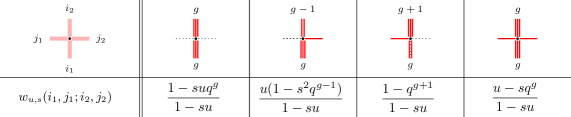
Figure 1. Vertex weights $w_{u,s}$. Here $i_{1},i_{2}\in\mathbb{Z}_{\geq 0}$ and $j_{1},j_{2}\in\left\{0,1\right\}$.

We will also use dual weights $w_{v,s}^{*}$ defined as

$$w_{v,s}^{*}(i_{1},j_{1};i_{2},j_{2})=\frac{(s^{2};q)_{i_{1}}(q;q)_{i_{2}}}{(s^{2};q)_{i_{2}}(q;q)_{i_{1}}}\,w_{v,s}(i_{2},j_{1};i_{1},j_{2}).$$ (2.1)

They are given in Figure 2. The arrow preservation here reads $i_{2}+j_{1}=i_{1}+j_{2}$, and so we think of occupied edges as forming up-left paths.

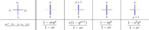
Figure 2. Dual vertex weights $w^{*}_{v,s}$. Here $i_{1},i_{2}\in\mathbb{Z}_{\geq 0}$ and $j_{1},j_{2}\in\left\{0,1\right\}$.

2.2. Yang–Baxter equation

The weights $w_{u,s}$ and $w^{*}_{v,s}$ are very special in that they satisfy a Yang–Baxter (RLL type) equation. To write it down, we need additional cross vertex weights $R_{z}$ which also depend on $q$ (but not on the spin parameter $s$). The weights $R_{z}$ are given in Figure 3.

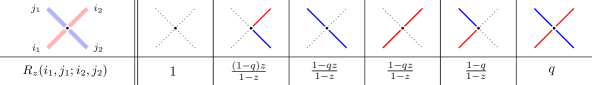
Figure 3. Cross vertex weights $R_{z}$. We have $i_{1},j_{1},i_{2},j_{2}\in\left\{0,1\right\}$. It is convenient to think that the red edges (labeled $i_{1},i_{2}$) are directed to the right, while the blue edges (labeled $j_{1},j_{2}$) are directed to the left.

Proposition 2.1 (Yang–Baxter equation).

For any $i_{1},i_{2},j_{1},j_{2}\in\left\{0,1\right\}$ and $i_{3},j_{3}\in\mathbb{Z}_{\geq 0}$ we have

$$\begin{split}&\sum_{k_{1},k_{2},k_{3}}R_{uv}(i_{2},i_{1};k_{2},k_{1})\,w^{*}_{v,s}(i_{3},k_{1};k_{3},j_{1})\,w_{u,s}(k_{3},k_{2};j_{3},j_{2})\\ &\hskip 100.0pt=\sum_{k^{\prime}_{1},k^{\prime}_{2},k^{\prime}_{3}}w^{*}_{v,s}(k^{\prime}_{3},i_{1};j_{3},k^{\prime}_{1})\,w_{u,s}(i_{3},i_{2};k^{\prime}_{3},k^{\prime}_{2})\,R_{uv}(k^{\prime}_{2},k^{\prime}_{1};j_{2},j_{1}).\end{split}$$ (2.2)

The sum in left-hand side of (2.2) goes over $k_{1},k_{2}\in\left\{0,1\right\}$ and $k_{3}\in\mathbb{Z}_{\geq 0}$, and similarly for the right-hand side. See Figure 4 for an illustration.

Proof.

The Yang–Baxter equation (2.2) can be verified directly by considering 16 cases for $i_{1},i_{2},j_{1},j_{2}\in\left\{0,1\right\}$ and arbitrary $i_{3},j_{3}\in\mathbb{Z}_{\geq 0}$. See [BP19, Appendix B] for an explicit listing of similar identities, and [Bor17] or [Man14, (4.8)] for discussions of how the Yang–Baxter equation arises from quantum integrability. ∎

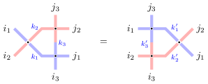
Figure 4. Graphical illustration of the Yang–Baxter equation (2.2). In the left-hand side, the weight $w_{u,s}$ is at the top, and $w_{v,s}^{*}$ is at the bottom. The weights are switched in the right-hand side.

The cross vertex weights $R_{uv}$ in (2.2) do not depend on $s$. Moreover, they depend on the spectral parameters $u,v$ attached to the vertices $w_{u,s}$ and $w_{v,s}^{*}$ only through their product $uv$. Therefore, the same Yang–Baxter equation (with the same $R_{uv}$) holds for a whole family of weights $(w_{u\xi,s},w_{v/\xi,s}^{*})$, where both $\xi$ and $s$ are arbitrary. We use this flexibility in the next section to define fully inhomogeneous spin Hall–Littlewood symmetric rational functions.

2.3. Spin Hall–Littlewood symmetric functions

Spin Hall–Littlewood symmetric functions are indexed by signatures. We refer to Section 1.7 for notation related to signatures. Here we need only nonnegative signatures.

Fix $q$, spin parameters $s_{x}$ and inhomogeneity parameters $\xi_{x}$, where $x=0,1,2,\ldots$ is the horizontal coordinate. We define the spin Hall–Littlewood function $\mathsf{F}_{\lambda}(u_{1},\ldots,u_{N})$, $\lambda\in\mathrm{Sign}_{N}$, as the partition function of up-right path ensembles in $\mathbb{Z}_{\geq 0}\times\left\{1,\ldots,N\right\}$, such that:

1. A path enters the region at each location $(0,i)$, $i=1,\ldots,N$, on the left boundary;

2. A path exits the region at locations $(\lambda_{j},N)$, $j=1,\ldots,N$ on the top boundary (multiple paths may exit through the same vertical edge);

3. No paths enter through the bottom boundary or escape to infinity far to the right;

4. At each vertex $(x,i)$, $x\in\mathbb{Z}_{\geq 0}$, $i\in\left\{1,\ldots,N\right\}$, the vertex weight is taken to be $w_{u_{i}\xi_{x},s_{x}}$.

See Figure 5 (left) for an illustration. Note that this partition function is well-defined since the weight of the empty vertex is $w_{u,s}(0,0;0,0)=1$. By the very definition, $\mathsf{F}_{\lambda}(u_{1},\ldots,u_{N})$ is a rational function of the variables $u_{i}$ as well as of all parameters. The functions $\mathsf{F}_{\lambda}$ appeared in [Bor17] in the homogeneous case $\xi_{x}\equiv 1$, $s_{x}\equiv s$, and the inhomogeneous generalization is performed in [BP18].

The dual spin Hall–Littlewood functions are defined in a similar way using the weights $w^{*}_{v_{i}/\xi_{x},s_{x}}$ and ensembles of up-left paths, see Figure 5 (right) for an illustration. (Note that in [Bor17], [BP18] the functions $\mathsf{F}^{*}_{\lambda}$ were denoted by $\mathsf{F}^{\mathsf{c}}_{\lambda}$.)

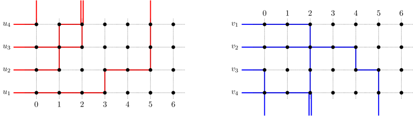
Figure 5. Left: An example of a path configuration contributing to the partition function $\mathsf{F}_{\lambda}(u_{1},u_{2},u_{3},u_{4})$, where $\lambda=(5,2,2,0)\in\mathrm{Sign}_{4}$. Right: An example of a path configuration for $\mathsf{F}^{*}_{\lambda}(v_{1},v_{2},v_{3},v_{4})$ with the same $\lambda$.

2.4. Properties of spin Hall–Littlewood functions

Here we summarize some properties of the spin Hall–Littlewood functions $\mathsf{F}_{\lambda},\mathsf{F}^{*}_{\lambda}$. First, for any $\lambda\in\mathrm{Sign}_{N}$, the functions $\mathsf{F}_{\lambda}(u_{1},\ldots,u_{N})$ and $\mathsf{F}^{*}_{\lambda}(v_{1},\ldots,v_{N})$ are symmetric in their spectral parameters $u_{i}$ and $v_{j}$, respectively. This fact follows from the Yang–Baxter equation, cf. [Bor17, Theorem 3.6] or [BP18, Proposition 4.5].

Next, we can express the dual functions through the usual ones as follows:

$$\mathsf{F}^{*}_{\lambda}(v_{1},\ldots,v_{N})=\prod_{r\geq 0}\frac{(s_{r}^{2};q)_{m_{r}}}{(q;q)_{m_{r}}}\,\mathsf{F}_{\lambda}(v_{1},\ldots,v_{N})\Big{|}_{\text{$\xi_{x}\to\xi_{x}^{-1}$ for all $x$}},$$ (2.3)

where $\lambda=(0^{m_{0}}1^{m_{1}}2^{m_{2}}\ldots)$ in the multiplicative notation. This follows from relation (2.1) between $w_{v/\xi,s}$ and $w^{*}_{v/\xi,s}$ together with telescopic cancellations occurring in weights of path configurations.

The functions $\mathsf{F}_{\lambda}$ admit an explicit symmetrization formula. Let

$$\varphi_{k}(u):=\frac{1-q}{1-s_{k}\xi_{k}u}\prod_{j=0}^{k-1}\frac{\xi_{j}u-s}{1-s_{j}\xi_{j}u},\qquad k\geq 0.$$ (2.4)

Then [BP18, Theorem 4.14.1]

$$\mathsf{F}_{\lambda}(u_{1},\ldots,u_{N})=\sum_{\sigma\in S_{N}}\sigma\Biggl{(}\prod_{1\leq i<j\leq N}\frac{u_{i}-qu_{j}}{u_{i}-u_{j}}\,\prod_{i=1}^{N}\varphi_{\lambda_{i}}(u_{i})\Biggr{)},$$ (2.5)

where $S_{N}$ is the symmetric group, and $\sigma$ acts by permuting the $u_{i}$’s and not the $\lambda_{i}$’s. Formula (2.5) is nontrivial and follows from an application of the algebraic Bethe Ansatz. Consequently, via (2.3) the dual functions $\mathsf{F}^{*}_{\lambda}$ also possess a similar symmetrization formula:

$$\mathsf{F}^{*}_{\lambda}(v_{1},\ldots,v_{N})=\prod_{r\geq 0}\frac{(s_{r}^{2};q)_{m_{r}(\lambda)}}{(q;q)_{m_{r}(\lambda)}}\sum_{\sigma\in S_{N}}\sigma\Biggl{(}\prod_{1\leq i<j\leq N}\frac{v_{i}-qv_{j}}{v_{i}-v_{j}}\,\prod_{i=1}^{N}\biggl{(}\frac{1-q}{1-s_{\lambda_{i}}\xi_{\lambda_{i}}^{-1}v_{i}}\prod_{j=0}^{\lambda_{i}-1}\frac{\xi_{j}^{-1}v_{i}-s_{j}}{1-s_{j}\xi_{j}^{-1}v_{i}}\biggr{)}\Biggr{)}.$$ (2.6)

The functions $\mathsf{F}_{\lambda}$ satisfy a Cauchy type identity together with another family of functions denoted by $\mathsf{G}_{\lambda}^{*}(v_{1},\ldots,v_{M})$. The $\mathsf{G}_{\lambda}^{*}$’s are partition functions of configurations as in Figure 5 (right) with weights $w^{*}_{v_{i}/\xi_{x},s_{x}}$, but with different boundary conditions: the exiting paths all exit vertically through $(0,N)$ instead of horizontally. We refer to [BP18, Section 4.3] for details on the functions $\mathsf{G}^{*}_{\lambda}$, see also Section 5.6 below for an explicit symmetrization formula for $\mathsf{G}_{\lambda}^{*}$. The Cauchy type identity reads [BP18, Corollary 4.13]

$$\sum_{\lambda\in\mathrm{Sign}_{N}}\mathsf{F}_{\lambda}(u_{1},\ldots,u_{N})\,\mathsf{G}^{*}_{\lambda}(v_{1},\ldots,v_{M})=\frac{(q;q)_{N}}{\prod_{i=1}^{N}(1-s_{0}\xi_{0}u_{i})}\,\prod_{i=1}^{N}\prod_{j=1}^{M}\frac{1-qu_{i}v_{j}}{1-u_{i}v_{j}},$$ (2.7)

provided that the variables satisfy

$$\left|\frac{\xi_{x}u_{i}-s_{x}}{1-s_{x}\xi_{x}u_{i}}\cdot\frac{v_{j}/\xi_{x}-s_{x}}{1-s_{x}v_{j}/\xi_{x}}\right|\leq 1-\varepsilon<1\qquad\textnormal{for all $i,j$ and all $x=0,1,2,\ldots$.}$$ (2.8)

Note that when $\xi_{x}>0$, $-1<s_{x}\leq 0$, and $u_{i},v_{j}>0$, condition (2.8) follows from $u_{i}v_{j}\leq 1-\varepsilon^{\prime}<1$ (for a suitable choice of $\varepsilon^{\prime}>0$). Identity (2.7) follows from the Yang–Baxter equation.

The following torus orthogonality holds [BP18, Corollary 7.5]. Provided some technical conditions on the parameters (which are given in the cited statement and are not explicitly required for our purposes), for all $\lambda,\mu\in\mathrm{Sign}_{N}$ we have

$$\frac{1}{N!(2\pi\mathbf{i})^{N}}\oint du_{1}\ldots\oint du_{N}\,\frac{\prod_{i\neq j}(u_{i}-u_{j})}{\prod_{i,j=1}^{N}(u_{i}-qu_{j})}\,\mathsf{F}_{\lambda}(u_{1},\ldots,u_{N})\,\mathsf{F}_{\mu}^{*}(u_{1}^{-1},\ldots,u_{N}^{-1})=\mathbf{1}_{\lambda=\mu},$$ (2.9)

where each integration is over the same positively oriented simple closed contour $C$ encircling all $s_{x}q^{j}/\xi_{x}$ (where $x\geq 0$, $0\leq j\leq N-1$), and such that $C$ encircles the contour $qC$ (the image of $C$ under the multiplication by $q$).

We also have an orthogonality relation of another type:

$$\begin{split}&\sum_{-\infty<\lambda_{N}\leq\lambda_{N-1}\leq\ldots\leq\lambda_{1}<+\infty}\mathsf{F}_{\lambda}(u_{1},\ldots,u_{N})\,\mathsf{F}_{\lambda}^{*}(v_{1}^{-1},\ldots,v_{N}^{-1})\\ &\hskip 100.0pt=(-1)^{\frac{N(N-1)}{2}}\frac{\prod_{i,j=1}^{N}(u_{i}-qv_{j})}{\prod_{1\leq i<j\leq N}(u_{i}-u_{j})(v_{i}-v_{j})}\,\det\left[\delta(v_{i}-u_{j})\right]_{i,j=1}^{N}.\end{split}$$ (2.10)

Here $\delta(\cdot)$ is the Dirac delta, and identity (2.10) should be understood in an integral sense (we refer to [BP18, Theorem 7.7] for detailed formulation and proof). Note also that the summation in the left-hand side of (2.10) is over signatures $\lambda$ which are not necessarily nonnegative. For signatures with possibly negative parts, we trivially extend the definition of $\mathsf{F}_{\lambda}$ using the shifting property

$$\mathsf{F}_{(\lambda_{1}+r,\ldots,\lambda_{N}+r)}(u_{1},\ldots,u_{N})\\ =\prod_{i=1}^{N}\prod_{j=0}^{r-1}\frac{\xi_{j}u_{i}-s_{j}}{1-s_{j}\xi_{j}u_{i}}\left(\mathsf{F}_{(\lambda_{1},\ldots,\lambda_{N})}(u_{1},\ldots,u_{N})\Big{|}_{(\xi_{x},s_{x})\to(\xi_{x+r},s_{x+r})\ \text{for all $x$}}\right),$$

where $r\geq 1$, and similarly for the $\mathsf{F}^{*}_{\lambda}$’s.

In [BCPS15] and [BP18] the torus orthogonality (2.9) is called spatial, and (2.10) is referred to as the spectral orthogonality.

2.5. Stable spin Hall–Littlewood functions

A useful variant (in fact, a particular case) of the spin Hall–Littlewood functions was introduced in [GdGW17], [BW17]. The stable spin Hall–Littlewood functions $\widetilde{\mathsf{F}}_{\lambda}$, $\widetilde{\mathsf{F}}^{*}_{\lambda}$ are indexed by partitions $\lambda=(\lambda_{1}\geq\lambda_{2}\geq\ldots\geq\lambda_{\ell(\lambda)}>0)$ instead of signatures. That is, these functions only care about nonzero parts of $\lambda$, and the partition $\lambda$ may have an arbitrary length. The passage to the stable functions is done by inserting infinitely many incoming and outgoing vertical paths at location $0$. In particular, the resulting stable functions may depend on an arbitrary number of variables $k\geq\ell(\lambda)$, not tied with the length of the signature (if $k<\ell(\lambda)$, the stable function is zero, by agreement).

There are two ways to obtain stable functions indexed by a partition $\lambda=(\lambda_{1}\geq\ldots\geq\lambda_{\ell}>0)$. First, we have (cf. [BMP19, Section 3.3])

$$\widetilde{\mathsf{F}}_{\lambda}(u_{1},\ldots,u_{k})=\prod_{i=1}^{k}(1-s_{0}\xi_{0}u_{i})\cdot\lim_{m\to+\infty}\mathsf{F}_{\lambda\cup 0^{m+k-\ell}/0^{m}}(u_{1},\ldots,u_{k}),$$ (2.11)

where in the right-hand side we have signatures with growing numbers of zeroes. Alternatively,

$$\widetilde{\mathsf{F}}_{\lambda}(u_{1},\ldots,u_{k})=\frac{1}{(q;q)_{k-\ell}}\,\mathsf{F}_{\lambda\cup 0^{k-\ell}}(u_{1},\ldots,u_{k})\Big{|}_{s_{0}=0}.$$ (2.12)

Note that the stable functions $\widetilde{\mathsf{F}}_{\lambda}$ do not depend on $s_{0}$. While this is clear from (2.12), in (2.11) we needed the prefactor to cancel the corresponding denominators. We will mostly use the second way (2.12) and so refer to [BP18, Definitions 4.3 and 4.4] for the definition of the skew spin Hall–Littlewood functions $\mathsf{F}_{\lambda\cup 0^{m+k-\ell}/0^{m}}$.

Analogously, the dual stable functions are given by

$$\widetilde{\mathsf{F}}_{\lambda}^{*}(v_{1},\ldots,v_{k})=\prod_{i=1}^{k}(1-s_{0}v_{i}/\xi_{0})\cdot\lim_{m\to+\infty}\mathsf{F}_{\lambda\cup 0^{m+k-\ell}/0^{m}}^{*}(v_{1},\ldots,v_{k}),$$ (2.13)

or equivalently by

$$\widetilde{\mathsf{F}}_{\lambda}^{*}(v_{1},\ldots,v_{k})=\mathsf{F}_{\lambda\cup 0^{k-\ell}}^{*}(v_{1},\ldots,v_{k})\Big{|}_{s_{0}=0}.$$ (2.14)

The name “stable” comes from the fact that

$$\widetilde{\mathsf{F}}_{\lambda}(u_{1},\ldots,u_{k-1},0)=\widetilde{\mathsf{F}}_{\lambda}(u_{1},\ldots,u_{k-1}),$$

and similarly for the dual functions.

The stable spin Hall–Littlewood functions also satisfy the following Cauchy type identity:

Proposition 2.2 ([BW17, Corollary 7.6]).

If the variables satisfy (2.8), then

$$\sum_{\lambda}\widetilde{\mathsf{F}}_{\lambda}(u_{1},\ldots,u_{n})\,\widetilde{\mathsf{F}}_{\lambda}^{*}(v_{1},\ldots,v_{m})=\prod_{i=1}^{n}\prod_{j=1}^{m}\frac{1-qu_{i}v_{j}}{1-u_{i}v_{j}},$$ (2.15)

where the sum runs over all partitions $\lambda=(\lambda_{1}\geq\ldots\geq\lambda_{\ell(\lambda)}>0)$ of arbitrary length.

3. Refined Cauchy identity. Proof of Theorem 1.2

In this section we use the Yang–Baxter equation and Lagrange interpolation method to establish our first main result, Theorem 1.2.

3.1. Two partition functions

We begin by defining two partition functions depending on an integer $N$, spectral parameters $u_{1},\ldots,u_{N}$, $v_{1},\ldots,v_{N}$, other parameters $q,s_{x},\xi_{x}$ of the model, and an additional integer $a\in\left\{0,1,2,\ldots\right\}\cup\left\{+\infty\right\}$. For future use we also denote $\gamma:=q^{a}$ (when $a=+\infty$, we have $\gamma=0$), and treat $\gamma$ as a generic complex parameter. This is possible because, as we observe throughout the computations, our quantities of interest, $\mathscr{Z}^{q^{a}}_{N}$ (Definition 3.1) and $\mathscr{S}^{q^{a}}_{N}$ (Definition 3.2), are rational functions of $q^{a}$. Hence these quantities admit a meromorphic continuation in the variable $\gamma=q^{a}$.

Definition 3.1 (Domain wall type partition function).

Denote by

$$\mathscr{Z}^{\gamma}_{N}=\mathscr{Z}^{\gamma}_{N}(u_{1},\ldots,u_{N}\mid v_{1},\ldots,v_{N};s_{0})$$

the partition function of the cross vertex configuration as in Figure 6 (left), where the cross vertex weights are $R_{u_{i}v_{j}}$, and the weights on the right are $w_{u_{i}\xi_{0},s_{0}}$ and $w^{*}_{v_{j}/\xi_{0},s_{0}}$. The boundary conditions are $1$’s on the left, $0$’s on the right, and there are $a$ vertical arrows entering from below and exiting from the top.

When $a=0$ (that is, $\gamma=1$), we can ignore the vertical column of vertices on the right, and so $\mathscr{Z}^{\gamma=1}_{N}$ essentially becomes the partition function of the inhomogeneous six vertex model with weights $R_{u_{i}v_{j}}$ (given in Figure 3) and domain wall boundary conditions. For general $a\neq 0$ (that is, for $\gamma\neq 1$) we may call the boundary conditions the decorated domain wall. The decorated boundary conditions depend on three extra parameters, $s_{0}$, $\xi_{0}$, and $\gamma=q^{a}$.

Definition 3.2 (Refined Cauchy partition function).

Assume that the spectral parameters $u_{i},v_{j}$ satisfy (2.8). Denote by

$$\mathscr{S}^{\gamma}_{N}=\mathscr{S}^{\gamma}_{N}(u_{1},\ldots,u_{N}\mid v_{1},\ldots,v_{N};s_{0})$$

the partition function of the vertex configuration as in Figure 6 (right). Here the vertex weights in the bottom part are $w_{u_{i}\xi_{x},s_{x}}$ and the weights in the top part are $w_{v_{j}/\xi_{x},s_{x}}^{*}$. The boundary conditions are $1$ on the left, $0$ on the right and everywhere at the top and the bottom except the zeroth column. In the zeroth column, there are $a$ arrows entering from the bottom and exiting from the top.

Note that the number of configurations contributing to $\mathscr{Z}_{N}^{\gamma}$ is finite, while this number is infinite for $\mathscr{S}_{N}^{\gamma}$. Hence the need for the convergence condition (2.8) in Definition 3.2. Also, we explicitly indicate the dependence of the partition functions $\mathscr{Z}^{\gamma}_{N}$ and $\mathscr{S}^{\gamma}_{N}$ on $s_{0}$ for future convenience, as in some formulas we would like to change the value of $s_{0}$. Since all other parameters $\xi_{0}$ and $(s_{x},\xi_{x})$, $x\geq 1$, remain the same, we do not indicate them in the notation.

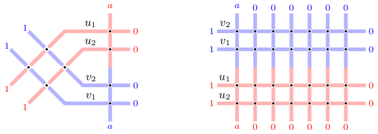
Figure 6. Boundary conditions and spectral parameters corresponding to the partition functions $\mathscr{Z}^{\gamma}_{N}$ (left) and $\mathscr{S}^{\gamma}_{N}$ (right) with $N=2$. The cross vertex weights are $R_{u_{i}v_{j}}$, and the grid vertex weights are $w_{u_{i}\xi_{x},s_{x}}$ (red) and $w^{*}_{v_{i}/\xi_{x},s_{x}}$ (blue).

Remark 3.3.

Using skew spin Hall–Littlewood functions (we refer to [BP18, Definitions 4.3 and 4.4] for their definition), we can write

$$\mathscr{S}^{\gamma}_{N}(u_{1},\ldots,u_{N}\mid v_{1},\ldots,v_{N};s_{0})=\sum_{\lambda\in\mathrm{Sign}_{N}}\mathsf{F}_{\lambda\cup 0^{a}/0^{a}}(u_{1},\ldots,u_{N})\,\mathsf{F}^{*}_{\lambda\cup 0^{a}/0^{a}}(v_{1},\ldots,v_{N}).$$

3.2. Refined Cauchy type sum

Here we deal with the refined Cauchy type sum $\mathscr{S}^{\gamma}_{N}$, and rewrite it in terms of the spin Hall–Littlewood functions. The resulting expression would look similar to the left-hand sides of the known Cauchy identities (2.7), (2.15), but with a new refinement factor.

Proposition 3.4.

Let the parameters $u_{i},v_{j}$ satisfy (2.8). When $\gamma\neq 0$, we have

$$\begin{split}&\mathscr{S}_{N}^{\gamma}(u_{1},\ldots,u_{N}\mid v_{1},\ldots,v_{N};\gamma^{-1}s_{0})=\prod_{j=1}^{N}\frac{1-\xi_{0}s_{0}u_{j}}{1-\xi_{0}s_{0}\gamma^{-1}u_{j}}\,\frac{1-s_{0}v_{j}/\xi_{0}}{1-s_{0}\gamma^{-1}v_{j}/\xi_{0}}\\ &\hskip 60.0pt\times\sum_{\lambda\in\mathrm{Sign}_{N}}\frac{(\gamma q;q)_{N-\ell(\lambda)}}{(q;q)_{N-\ell(\lambda)}}\frac{(\gamma^{-1}s_{0}^{2};q)_{N-\ell(\lambda)}}{(s_{0}^{2};q)_{N-\ell(\lambda)}}\,\mathsf{F}_{\lambda}(u_{1},\ldots,u_{N})\,\mathsf{F}^{*}_{\lambda}(v_{1},\ldots,v_{N}).\end{split}$$ (3.1)

Here in the right-hand side the spin Hall–Littlewood functions $\mathsf{F}_{\lambda},\mathsf{F}_{\lambda}^{*}$ contain the original parameter $s_{0}$. Moreover, for $\gamma=0$ we have

$$\begin{split}&\mathscr{S}^{\gamma=0}_{N}(u_{1},\ldots,u_{N}\mid v_{1},\ldots,v_{N};s_{0})=\prod_{j=1}^{N}\frac{1}{(1-s_{0}\xi_{0}u_{j})(1-s_{0}v_{j}/\xi_{0})}\\ &\hskip 180.0pt\times\sum_{\nu}\widetilde{\mathsf{F}}_{\nu}(u_{1},\ldots,u_{N})\,\widetilde{\mathsf{F}}^{*}_{\nu}(v_{1},\ldots,v_{N}),\end{split}$$ (3.2)

where the sum is over partitions $\nu$ of length at most $N$, and $\widetilde{\mathsf{F}}_{\nu},\widetilde{\mathsf{F}}^{*}_{\nu}$ are the stable spin Hall–Littlewood functions.

Proof.

Throughout the proof we assume that $a\geq N$, so that no negative arrow numbers occur in the partition function, and no configurations are forbidden. As the resulting identity depends on $\gamma=q^{a}$ in a rational way (due to (2.8) all infinite sums converge, and are equal to rational functions), this assumption does not restrict the generality.

Fix an arbitrary path configuration contributing to the partition function $\mathscr{S}^{\gamma}_{N}$. Let $\lambda\in\mathrm{Sign}_{N}$ encode the intermediate arrow configuration between the red and the blue parts. In the bottom (red) part of Figure 6 (right), the number of arrows in the zeroth column at height $N$ is equal to $a+N-\ell(\lambda)$, where $\ell(\lambda)$ is the number of nonzero parts in $\lambda$. Apart from the zeroth column, the weights $w_{u_{j}\xi_{x},s_{x}}$, $x\geq 1$, of all vertices are the same as in the definition of $\mathsf{F}_{\lambda}(u_{1},\ldots,u_{N})$. In the zeroth column, there are two types of vertices, and their weights depend on $\gamma$ in the following way:

$$\begin{split}w_{u_{j}\xi_{0},s_{0}/\gamma}(a+i,1;a+i,1)=\frac{\xi_{0}u_{j}-s_{0}q^{i}}{1-\xi_{0}s_{0}u_{j}/\gamma},\\ w_{u_{j}\xi_{0},s_{0}/\gamma}(a+i,1;a+i+1,0)=\frac{1-\gamma q^{i+1}}{1-\xi_{0}s_{0}u_{j}/\gamma}.\end{split}$$ (3.3)

Let us first look at the numerators in (3.3). The number of vertices of type $(a+i,1;a+i+1,0)$ is equal to $N-\ell(\lambda)$, since only $\ell(\lambda)$ paths leave the zeroth column. These vertices correspond to the number $i$ ranging from $0$ to $N-\ell(\lambda)-1$. We see that by taking out the prefactor $\frac{(\gamma q;q)_{N-\ell(\lambda)}}{(q;q)_{N-\ell(\lambda)}}$ from the weight of the whole path configuration, we may remove the $\gamma$-modification from the numerators of the weights of the second type of vertices in (3.3).

It remains to remove the $\gamma$-modification from the denominators in (3.3), and this is achieved by taking out the factor

$$\prod_{i=1}^{N}\frac{1-\xi_{0}s_{0}u_{j}}{1-\xi_{0}s_{0}\gamma^{-1}u_{j}}.$$

The resulting vertex weights are the same as the ones entering $\mathsf{F}_{\lambda}$. Therefore, for fixed $\lambda$ the partition function of the bottom (red) part in Figure 6 (right) is equal to

$$\frac{(\gamma q;q)_{N-\ell(\lambda)}}{(q;q)_{N-\ell(\lambda)}}\prod_{j=1}^{N}\frac{1-\xi_{0}s_{0}u_{j}}{1-\xi_{0}s_{0}\gamma^{-1}u_{j}}\,\mathsf{F}_{\lambda}(u_{1},\ldots,u_{N}).$$

For the top (blue) part in Figure 6 (right) we argue in a similar way by relating the partition function of the top part to $\mathsf{F}^{*}_{\lambda}(v_{1},\ldots,v_{N})$. In the zeroth column, there are two types of vertices with weights depending on $\gamma$ as

$$\begin{split}w^{*}_{v_{j}/\xi_{0},s_{0}/\gamma}(a+i,1;a+i,1)&=\frac{v_{j}/\xi_{0}-s_{0}q^{i}}{1-s_{0}\gamma^{-1}v_{j}/\xi_{0}},\\ w^{*}_{v_{j}/\xi_{0},s_{0}/\gamma}(a+i+1,1;a+i,0)&=\frac{1-s_{0}^{2}\gamma^{-1}q^{i}}{1-s_{0}\gamma^{-1}v_{j}/\xi_{0}}.\end{split}$$ (3.4)

Similarly to the bottom part, we first take out the factor $\frac{(s_{0}^{2}\gamma^{-1};q)_{N-\ell(\lambda)}}{(s_{0}^{2};q)_{N-\ell(\lambda)}}$ which deals with the numerators in the vertex weights of the second type in (3.4). Then, to compensate for the denominators, we take out a suitable product over $j=1,\ldots,N$. This implies that for fixed $\lambda$ the partition function of the top (blue) part in Figure 6 (right) is equal to

$$\frac{(\gamma^{-1}s_{0}^{2};q)_{N-\ell(\lambda)}}{(s_{0}^{2};q)_{N-\ell(\lambda)}}\prod_{j=1}^{N}\frac{1-s_{0}v_{j}/\xi_{0}}{1-s_{0}\gamma^{-1}v_{j}/\xi_{0}}\,\mathsf{F}^{*}_{\lambda}(v_{1},\ldots,v_{N}).$$

Putting all together and summing over $\lambda$, we get the first claim.

The second claim follows from the definition of the stable spin Hall–Littlewood functions (Section 2.5) via inserting infinitely many arrows in the zeroth column. Indeed, setting $\gamma=0$ corresponds to $a=+\infty$. ∎

3.3. Equality of partition functions

Next we use the Yang–Baxter equation to relate the partition functions $\mathscr{Z}^{\gamma}_{N}$ and $\mathscr{S}^{\gamma}_{N}$.

Proposition 3.5.

We have

$$\mathscr{Z}^{\gamma}_{N}(u_{1},\ldots,u_{N}\mid v_{1},\ldots,v_{N};s_{0})=\mathscr{S}^{\gamma}_{N}(u_{1},\ldots,u_{N}\mid v_{1},\ldots,v_{N};s_{0})$$

provided that the spectral parameters $u_{i},v_{j}$ satisfy (2.8).

Proof.

Start with the configuration of the lattice corresponding to $\mathscr{Z}^{\gamma}_{N}$. Drag all the cross vertices to the right using the Yang–Baxter equation (Proposition 2.1). Condition (2.8) ensures that after moving the crosses, the end state of the cross vertices is $(0,0;0,0)$. Indeed, keeping the other eventual state $(1,1;0,0)$ of the cross vertex introduces infinitely many factors of the form $w_{u_{i}\xi_{x},s_{x}}(0,1;0,1)w_{u_{j}/\xi_{x},s_{x}}(0,1;0,1)$ into the weight of the path configuration. Condition (2.8) implies that each of these factors is smaller than $1-\varepsilon$ in the absolute value. Thus, configurations with the eventual state $(1,1;0,0)$ of the cross vertex do not contribute to the partition function. Finally, the fact that $R_{u_{i}v_{j}}(0,0;0,0)=1$ means that we arrive at the partition function $\mathscr{S}^{\gamma}_{N}$, and so the equality of partition functions follows. ∎

3.4. Evaluation of the Izergin–Korepin type determinant $\mathscr{Z}_{N}^{\gamma}$

The third and final step of the proof of Theorem 1.2 consists in an explicit computation (in a determinantal form) of the partition function of the six vertex model with the decorated domain wall boundary conditions. We compute it by the Lagrange interpolation technique (similarly to, e.g., [WZJ16]).

3.4.1. Formulation of the result

Denote

$$\mathsf{z}(u,v;s_{0}):=\frac{(1-\gamma)(q-\gamma s_{0}^{2})(1-uv)+(1-q)(1-\gamma\xi_{0}s_{0}u)(1-\gamma\xi_{0}^{-1}s_{0}v)}{(1-uv)(1-quv)}.$$ (3.5)

Proposition 3.6.

We have

$$\begin{split}&\mathscr{Z}^{\gamma}_{N}(u_{1},\ldots,u_{N}\mid v_{1},\ldots,v_{N};s_{0})\\ &\hskip 30.0pt=\prod_{j=1}^{N}\frac{1}{(1-s_{0}\xi_{0}u_{j})(1-\xi_{0}^{-1}s_{0}v_{j})}\,\frac{\prod_{i,j=1}^{N}(1-qu_{i}v_{j})}{\prod_{1\leq i<j\leq N}(u_{i}-u_{j})(v_{i}-v_{j})}\,\det\left[\mathsf{z}(u_{i},v_{j};s_{0})\right]_{i,j=1}^{N}.\end{split}$$ (3.6)

Before proving Proposition 3.6, let us discuss three reductions.

First, when $s_{0}=0$, this result is established in [WZJ16, Lemma 5].

Next, keeping $s_{0}$ generic and setting $\gamma=1$ (that is, $a=0$), we have

$$\mathscr{Z}^{\gamma=1}_{N}(u_{1},\ldots,u_{N}\mid v_{1},\ldots,v_{N})=\frac{(1-q)^{N}\prod_{i,j=1}^{N}(1-qu_{i}v_{j})}{\prod_{1\leq i<j\leq N}(u_{i}-u_{j})(v_{i}-v_{j})}\,\det\left[\frac{1}{(1-u_{i}v_{j})(1-qu_{i}v_{j})}\right]_{i,j=1}^{N}.$$ (3.7)

The determinant in the right-hand side is the celebrated Izergin–Korepin determinant [Ize87], [KBI93, Ch. VII.10].

Third, keep $s_{0}$ generic, and consider now the case $\gamma=0$. We have

$$\mathsf{z}(u,v;s_{0})\big{|}_{\gamma=0}=\frac{q(1-uv)+(1-q)}{(1-uv)(1-quv)}=\frac{1}{1-uv}.$$

Thus, for $\gamma=0$ the partition function $\mathscr{Z}_{N}^{\gamma}(u_{1},\ldots,u_{N}\mid v_{1},\ldots,v_{N};s_{0})$ simplifies using the Cauchy determinant (e.g., [Mui23, vol. III, p. 311]) to

$$\mathscr{Z}^{\gamma}_{N}(u_{1},\ldots,u_{N}\mid v_{1},\ldots,v_{N};s_{0})\Big{|}_{\gamma=0}=\prod_{j=1}^{N}\frac{1}{(1-s_{0}\xi_{0}u_{j})(1-s_{0}v_{j}/\xi_{0})}\prod_{i,j=1}^{N}\frac{1-qu_{i}v_{j}}{1-u_{i}v_{j}}.$$ (3.8)

Formula (3.8) agrees with the known Cauchy identity for the stable spin Hall–Littlewood functions recalled in Proposition 2.2. To see this, use (3.2) and Proposition 3.5.

On the other hand, formula (3.8) for the six vertex model partition function may be obtained independently by noting that for $a=+\infty$, the weights $w_{u_{j}\xi_{0},s_{0}}$ and $w^{*}_{v_{j}/\xi_{0},s_{0}}$ do not depend on the number of incoming horizontal arrows from the left, and

$$\sum_{i_{2},j_{2}}R_{uv}(i_{1},j_{1};i_{2},j_{2})=\frac{1-quv}{1-uv}$$

for all $i_{1},j_{1}$. Therefore, the decorated domain wall partition function factorizes. This independent derivation of (3.8) establishes Proposition 3.6 for $\gamma=0$.

The proof of Proposition 3.6 in the case of general $\gamma$ occupies the rest of this subsection. We argue using Lagrange interpolation technique (similarly to, e.g., [WZJ16]) which consists of three steps. First, directly from Definition 3.1 we formulate five properties which the partition function $\mathscr{Z}^{\gamma}_{N}$ satisfies. Then we show that these properties determine a function uniquely. Finally, we check that the determinantal formula in the right-hand side of (3.6) satisfies the same five properties, which establishes the desired equality.

3.4.2. Step 1. Properties of the partition function

Denote

$$\widetilde{\mathscr{Z}}^{\gamma}_{N}(u_{1},\ldots,u_{N}\mid v_{1},\ldots,v_{N};s_{0})\\ :=\prod_{j=1}^{N}(1-s_{0}\xi_{0}u_{j})(1-\xi_{0}^{-1}s_{0}v_{j})\prod_{i,j=1}^{N}(1-u_{i}v_{j})\,\mathscr{Z}^{\gamma}_{N}(u_{1},\ldots,u_{N}\mid v_{1},\ldots,v_{N};s_{0}).$$

Additional factors in $\widetilde{\mathscr{Z}}^{\gamma}_{N}$ clear out all the denominators in the vertex weights $w_{u_{i}\xi_{0},s_{0}}$, $w^{*}_{v_{j}/\xi_{0},s_{0}}$, and $R_{u_{i}v_{j}}$, $i,j=1,\ldots,N$. This means that $\widetilde{\mathscr{Z}}^{\gamma}_{N}$ now depends on the spectral parameters $u_{i},v_{j}$ in a polynomial manner. As the first step in the proof of Proposition 3.6, let us list a number of properties of this renormalized partition function $\widetilde{\mathscr{Z}}^{\gamma}_{N}$.

Properties 3.7.

1. The function $\widetilde{\mathscr{Z}}^{\gamma}_{N}(u_{1},\ldots,u_{N}\mid v_{1},\ldots,v_{N};s_{0})$ is symmetric separately in each of the two sets of variables $\left\{u_{1},\ldots,u_{N}\right\}$ and $\left\{v_{1},\ldots,v_{N}\right\}$.

2. As a function of each single variable $u_{i}$ or $v_{j}$, $\widetilde{\mathscr{Z}}^{\gamma}_{N}(u_{1},\ldots,u_{N}\mid v_{1},\ldots,v_{N};s_{0})$ is a polynomial of degree at most $N$.

3. Setting $u_{1}=v_{1}^{-1}$, we have the recurrence

   $$\begin{split}&\widetilde{\mathscr{Z}}^{\gamma}_{N}(u_{1},u_{2},\ldots,u_{N}\mid v_{1},v_{2},\ldots,v_{N};s_{0})\Big{|}_{u_{1}=v_{1}^{-1}}\\ &\hskip 50.0pt=(1-q)(1-s_{0}\xi_{0}\gamma v_{1}^{-1})(1-s_{0}\xi_{0}^{-1}\gamma v_{1})\prod_{j=2}^{N}\left(1-qv_{1}^{-1}v_{j}\right)\left(1-qv_{1}u_{j}\right)\\ &\hskip 100.0pt\times\widetilde{\mathscr{Z}}^{\gamma}_{N-1}(u_{2},\ldots,u_{N}\mid v_{2},\ldots,v_{N};s_{0}).\end{split}$$ (3.9)

4. Under the specialization $u_{j}=q^{j-1}/(s_{0}\xi_{0}\gamma)$, we have

   $$\begin{split}&\widetilde{\mathscr{Z}}^{\gamma}_{N}\left((s_{0}\xi_{0}\gamma)^{-1},q(s_{0}\xi_{0}\gamma)^{-1},\ldots,q^{N-1}(s_{0}\xi_{0}\gamma)^{-1}\mid v_{1},\ldots,v_{N};s_{0}\right)\\ &\hskip 80.0pt=q^{N^{2}}\prod_{i,j=1}^{N}\left(1-v_{i}\frac{q^{j-1}}{s_{0}\xi_{0}\gamma}\right)\prod_{j=1}^{N}(1-\gamma q^{-j+1})(1-s_{0}^{2}\gamma q^{-j}).\end{split}$$ (3.10)

5. For $N=1$, we have

   $$\widetilde{\mathscr{Z}}^{\gamma}_{1}(u\mid v;s_{0})=(1-\gamma)(q-\gamma s_{0}^{2})(1-uv)+(1-q)(1-\gamma\xi_{0}s_{0}u)(1-\gamma\xi_{0}^{-1}s_{0}v).$$ (3.11)

Properties 3, 4, and 5 follow from the definition of the renormalized partition function $\widetilde{\mathscr{Z}}^{\gamma}_{N}$. Namely, for 3, setting $u_{1}=v_{1}^{-1}$ makes the renormalized weight $(1-u_{1}v_{1})R_{u_{1}v_{1}}(1,1;1,1)$ disappear, and so the nontrivial behavior of the paths reduces to a square of size $N-1$. The factors in the right-hand side of (3.9) come from the “frozen” vertices. For 4, specializing the $u_{j}$ variables forces the configurations in the zeroth column to be of the form $(a-j,1;a-j+1,0)$, where $j=1,\ldots,N$ (here we assume $a\geq N$ which does not restrict the generality since the desired identity is between rational functions in $\gamma=q^{a}$). This requires all vertices inside the square to be of the type $(1,1;1,1)$, and thus we get the right-hand side of (3.10). For 5, identity (3.11) is straightforward.

Let us now prove properties 1 and 2.

Proof of symmetry.

Symmetry follows from a number of Yang–Baxter equations of a type different from the one in Proposition 2.1. Introduce vertex weights $r_{z}(i_{1},j_{1};i_{2},j_{2})$, $i_{1},i_{2},j_{1},j_{2}\in\left\{0,1\right\}$, given in Figure 7.

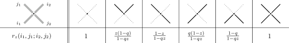
Figure 7. The vertex weights $r_{z}$ employed in the proof of symmetry of $\widetilde{\mathscr{Z}}^{\gamma}_{N}$.

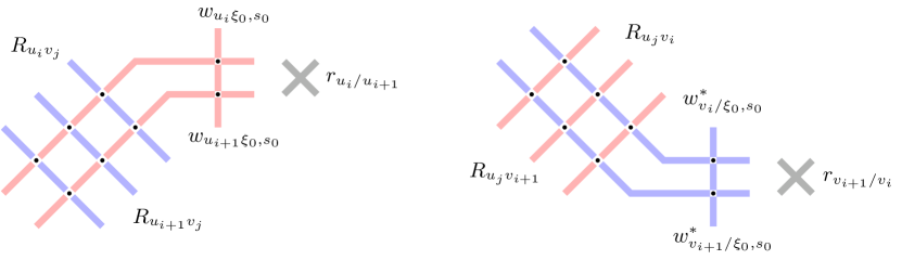
Figure 8. Interchanging spectral parameters $u_{i}\leftrightarrow u_{i+1}$ (left) or $v_{i}\leftrightarrow v_{i+1}$ (right) by means of Yang–Baxter equations involving weights $r_{z}$.

The fact that we can interchange the spectral parameters $u_{i},u_{i+1}$ follows from two Yang–Baxter equations. One is satisfied by the weights $r_{u_{i}/u_{i+1}},w_{u_{i}\xi_{0},s_{0}},w_{u_{i+1}\xi_{0},s_{0}}$, and the other one by $r_{u_{i}/u_{i+1}},R_{u_{i}v_{j}},R_{u_{i+1}v_{j}}$. These equations have a form similar to (2.2) and are illustrated in Figure 8 (left). This allows to take a cross vertex of weight $r_{u_{i}/u_{i+1}}$ and drag it throughout the lattice, interchanging the parameters $u_{i},u_{i+1}$ everywhere. The fact that we can interchange $v_{i},v_{i+1}$ follows similarly, see Figure 8 (right). All Yang–Baxter equations involved are verified in a straightforward way. ∎

Proof of polynomiality of degree $\leq N$.

Each variable $u_{i}$ and $v_{j}$ enters into $N+1$ vertices — $N$ cross vertices in the square, and one vertex in the zeroth column (cf. Figure 6, left). After renormalization, all vertex weights become linear in their respective spectral parameters. Thus, the degree of $\widetilde{\mathscr{Z}}^{\gamma}_{N}$ in each variable $u_{i}$ or $v_{j}$ is at most $N+1$. It remains to show that the coefficient by the $(N+1)$-st power is zero.

Due to symmetry, it suffices to consider only $u_{N}$ (the case of $v_{N}$ is analogous). In order to get a nonzero coefficient by $u_{N}^{N+1}$, the configuration of paths inside the $N\times N$ square should avoid weights $R_{u_{N}v_{j}}(1,1;0,0)$ because their renormalized weight equals $1-q$. This implies that in the zeroth column, the vertex containing the spectral parameter $u_{N}$ would be of type $(g,1;g+1,0)$. The renormalized weight of the latter vertex is $1-q^{g+1}$ which does not depend on $u_{N}$. We see that it is impossible to get a nonzero coefficient by $u_{N}^{N+1}$, so the total degree is at most $N$. ∎

3.4.3. Step 2. Uniqueness

The fact that 3.7 determine $\widetilde{\mathscr{Z}}^{\gamma}_{N}$ uniquely follows from Lagrange interpolation. For the reader’s convenience, let us reproduce the necessary statement which closely follows [WZJ16, Appendix B].

Lemma 3.8.

Let $f_{N}(u_{1},\dots,u_{N})$, $N\geq 1$, be symmetric polynomials in $(u_{1},\dots,u_{N})$ of degree at most $N$ in each $u_{j}$. Suppose that they satisfy recurrence

$$f_{N}(u_{1},\dots,u_{N-1},t_{i}) =C^{(i)}_{N}f_{N-1}(u_{1},\dots,u_{N-1}),\qquad 1\leq i\leq N,$$

for a suitable set of distinct points $\left\{t_{1},\dots,t_{N}\right\}$, where $C^{(i)}_{N}$ are some coefficients. Let also $f_{N}(u_{1}^{0},\ldots,u_{N}^{0})=C^{(0)}_{N}$ for some point $(u_{1}^{0},\ldots,u_{N}^{0})$ and some constant $C^{(0)}_{N}$.

If another family of symmetric polynomials $g_{N}(u_{1},\dots,u_{N})$, $N\geq 1$ satisfies all of these conditions and $f_{1}(u)=g_{1}(u)$, then

$$f_{N}(u_{1},\dots,u_{N})=g_{N}(u_{1},\dots,u_{N}),\quad\text{for all}\ N\geq 1.$$

Proof.

By induction, since $f_{1}=g_{1}$, we assume $f_{N-1}(u_{1},\ldots,u_{N-1})=g_{N-1}(u_{1},\ldots,u_{N-1})$. Then using the recurrence we see that $f_{N}(u_{1},\ldots,u_{N-1},t_{j})=g_{N}(u_{1},\ldots,u_{N-1},t_{j})$ for $N$ distinct points. This, together with the fact that the degree of $f_{N}$ in $u_{N}$ is at most $N$, implies that $f_{N}$ and $g_{N}$ coincide up to some constant factor (independent of $u_{N}$). Moreover, this constant factor cannot depend on $u_{1},\ldots,u_{N-1}$ either due to the symmetry of the polynomials. Finally, since $f_{N}$ and $g_{N}$ coincide at a fixed point $(u_{1}^{0},\ldots,u_{N}^{0})$, we get the claim. ∎

3.4.4. Step 3. Verification of properties for the determinantal formula

It remains to check that suitably normalized determinant in the right-hand side of (3.6) satisfies 3.7. This renormalization has the form

$$\frac{\prod_{i,j=1}^{N}(1-u_{i}v_{j})(1-qu_{i}v_{j})}{\prod_{1\leq i<j\leq N}(u_{i}-u_{j})(v_{i}-v_{j})}\,\det\left[\mathsf{z}(u_{i},v_{j};s_{0})\right]_{i,j=1}^{N},$$ (3.12)

where $\mathsf{z}(u,v;s_{0})$ is given by (3.5). Symmetry (property 1) is straightforward: permuting any pair $u_{i},u_{j}$ changes the sign of the determinant as well as the Vandermonde $\prod_{i<j}(u_{i}-u_{j})$ in the denominator. The fact that (3.12) is a polynomial of degree $N$ (property 2) follows because we can rewrite

$$\eqref{eq:Z_N_det_RHS}=\frac{1}{\prod_{1\leq i<j\leq N}(u_{i}-u_{j})(v_{i}-v_{j})}\,\det\Bigl{[}\mathsf{z}(u_{i},v_{j};s_{0})\prod_{l=1}^{N}(1-u_{i}v_{l})(1-qu_{i}v_{l})\Bigr{]}_{i,j=1}^{N},$$

and each element of the determinant is a polynomial in $u_{i}$ of degree $2N-1$. Dividing by the Vandermonde which has degree $N-1$ in each $u_{i}$ yields degree $N$.

Property 5 is straightforward.

For 3, we multiply the first row of the determinant by $1-u_{1}v_{1}$, and note that setting $u_{1}=1/v_{1}$ eliminates all elements in the first row except

$$(1-u_{1}v_{1})\,\mathsf{z}(u_{1},v_{1};s_{0})\big{|}_{u_{1}=v_{1}^{-1}}=(1-\gamma s_{0}v_{1}/\xi_{0})(1-\gamma s_{0}\xi_{0}/v_{1}).$$

This means that the determinant of size $N$ reduces to a similar determinant of size $N-1$ which is equal to $\widetilde{\mathscr{Z}}_{N-1}^{\gamma}$.

Finally, let us get property 4. Denote $u_{0}=(s_{0}\xi_{0}\gamma)^{-1}$.

Lemma 3.9.

The determinantal expression in (3.12), specialized at $u_{i}=u_{0}q^{i-1}$, $i=1,\ldots,N$, equals the right-hand side of (3.10).

Proof.

Take the $N\times N$ matrix $\mathsf{A}=[\mathsf{z}(u_{0}q^{j-1},v_{i};s_{0})]_{i,j=1}^{N}$ whose determinant we need to compute. We employ the method suggested in [Kra99, Section 2.6], and consider the LU decomposition $\mathsf{A}=\mathsf{L}\mathsf{U}$, where $\mathsf{L}$ is a lower triangular matrix with ones on the main diagonal, and $\mathsf{U}$ is an upper triangular matrix. (The fact that $\mathsf{A}$ is nondegenerate so that to admit an LU decomposition follows from the computations below.) Denote

$$f_{k}(v):=\prod_{r=1}^{k}(q^{r}v-\gamma s_{0}\xi_{0}),\qquad Q_{k}^{j}(v):=\frac{f_{k}(v)}{\prod_{r=1,\,r\neq j}^{k}(v-v_{r})}.$$ (3.13)

We claim that

$$(\mathsf{L}^{-1})_{ij}=\begin{cases}0,&i<j;\\ 1,&i=j;\\ -Q_{i-1}^{j}(v_{j})/Q_{i-1}^{j}(v_{i}),&i>j.\end{cases}$$

To see this, consider the product $\mathsf{L}^{-1}\mathsf{A}$ with $\mathsf{L}^{-1}$ being the candidate above. We would like to show that $\mathsf{L}^{-1}\mathsf{A}$ is upper triangular, that is,

$$\begin{split}\frac{f_{i-1}(v_{i})}{\prod_{r=1}^{i-1}(v_{i}-v_{r})}\,\mathsf{z}(u_{0}q^{j-1},v_{i};s_{0})&=\sum_{k=1}^{i-1}\frac{Q_{i-1}^{k}(v_{k})}{v_{i}-v_{k}}\,\mathsf{z}(u_{0}q^{j-1},v_{k};s_{0})\\ &=-\sum_{k=1}^{i-1}\frac{f_{i-1}(v_{k})}{\prod_{r=1,\,r\neq k}^{i}(v_{k}-v_{r})}\,\mathsf{z}(u_{0}q^{j-1},v_{k};s_{0}),\end{split}$$ (3.14)

for all $i>j$ (here the second equality is just a simplification using (3.13)). To show (3.14) we use the Residue Theorem. Consider the following function:

$$B(w):=\frac{f_{i-1}(w)}{\prod_{r=1}^{i}(w-v_{r})}\,\mathsf{z}(q^{j-1}u_{0},w;s_{0}),\qquad w\in\mathbb{C}.$$

It is a rational function with possible poles at $w=v_{1},\ldots,v_{i}$ and $w=q^{1-j}/u_{0},q^{-j}/u_{0}$ coming from $\mathsf{z}$ (3.5). However, since $i-1\geq j$, the zeroes coming from $f_{i-1}(w)$ (3.13) eliminate the two latter poles. Moreover, $B(w)$ is decaying as $O(1/w^{2})$ at infinity and thus has zero residue there. We see that (3.14) is simply an equality between the residue of $B(w)$ at $w=v_{i}$ and the sum of minus residues of $B(w)$ at all $w=v_{k}$, $k=1,\ldots,i-1$. This establishes (3.14).

Having the upper triangularity of $\mathsf{L}^{-1}\mathsf{A}$, we can compute the determinant as the product of diagonal elements:

$$\begin{split}\det\mathsf{A}=\det(\mathsf{L}^{-1}\mathsf{A})&=\prod_{i=1}^{N}\left(\mathsf{z}(u_{0}q^{i-1},v_{i};s_{0})-\sum_{k=1}^{i-1}\frac{Q_{i-1}^{k}(v_{k})}{Q_{i-1}^{k}(v_{i})}\,\mathsf{z}(u_{0}q^{i-1},v_{k};s_{0})\right)\\ &=\frac{\prod_{1\leq r<i\leq N}(v_{i}-v_{r})}{\prod_{i=1}^{N}f_{i-1}(v_{i})}\prod_{i=1}^{N}\frac{1}{2\pi\mathbf{i}}\oint_{c_{i}}\frac{f_{i-1}(w)\,\mathsf{z}(u_{0}q^{i-1},w;s_{0})}{\prod_{r=1}^{i}(w-v_{r})}\,dw,\end{split}$$

where the contour $c_{i}$ encircles $v_{1},\ldots,v_{i}$. Each $i$-th integrand is regular at infinity and has a single pole outside the contour $c_{i}$. This pole comes from $\mathsf{z}$ and is at $w=q^{-i}/u_{0}$. Taking the minus residues at these points gives a product formula for the determinant of $\mathsf{A}$. Putting all together, we arrive at the right-hand side of (3.10). ∎

This completes the proof of Proposition 3.6. Combining Propositions 3.6 and 3.4 we have established Theorem 1.2. Note that the parameter $s_{0}$ in (3.6) must be replaced by $s_{0}/\gamma$ to match the refined Cauchy sum, hence we get a slightly different determinant in Theorem 1.2.

4. Determinantal identity. Proof of Theorem 1.3

We will now present an alternative expression for the determinant in the right-hand side of the refined Cauchy identity. Recall the function $\mathsf{z}(u,v;s_{0})$ defined by (3.5), and also denote

$$\begin{split}&\mathsf{M}_{i}(v;\gamma^{-1}s_{0}):=\xi_{0}^{2i-N}v^{N-i-1}\\ &\hskip 20.0pt\times\left\{\left(1-s_{0}\xi_{0}^{-1}v\right)\left(v\xi_{0}^{-1}-s_{0}\right)\prod_{l=1}^{N}\frac{1-qvu_{l}}{1-vu_{l}}-\gamma^{-1}q^{N-i}\left(\gamma-s_{0}\xi_{0}^{-1}v\right)\left(\gamma qv\xi_{0}^{-1}-s_{0}\right)\right\};\\ &\widetilde{\mathsf{M}}_{i}(u;\gamma^{-1}s_{0}):=\\ &\hskip 20.0ptu^{N-i-1}\left\{\left(1-s_{0}\xi_{0}u\right)\left(u-\frac{s_{0}}{\xi_{0}}\right)\prod_{l=1}^{N}\frac{1-quv_{l}}{1-uv_{l}}-\gamma^{-1}q^{N-i}(\gamma-s_{0}\xi_{0}u)\left(\gamma qu-\frac{s_{0}}{\xi_{0}}\right)\right\}.\end{split}$$ (4.1)

The following result implies Theorem 1.3 from the Introduction.

Theorem 4.1.

We have

$$\begin{split}&\frac{\prod_{i,j=1}^{N}(1-qu_{i}v_{j})}{\prod_{1\leq i<j\leq N}(u_{i}-u_{j})(v_{i}-v_{j})}\,\det\left[\mathsf{z}(u_{i},v_{j};\gamma^{-1}s_{0})\right]_{i,j=1}^{N}\\ &\hskip 140.0pt=\frac{\det\bigl{[}\mathsf{M}_{i}(v_{j};\gamma^{-1}s_{0})\bigr{]}_{i,j=1}^{N}}{\prod_{1\leq i<j\leq N}(v_{i}-v_{j})}=\frac{\det\bigl{[}\widetilde{\mathsf{M}}_{i}(u_{j};\gamma^{-1}s_{0})\bigr{]}_{i,j=1}^{N}}{\prod_{1\leq i<j\leq N}(u_{i}-u_{j})}.\end{split}$$ (4.2)

Remark 4.2.

Recall that the right-hand side of the refined Cauchy identity in Theorem 1.2 is equal to

$$\prod_{j=1}^{N}\frac{1}{(1-s_{0}\xi_{0}u_{j})(1-\xi_{0}^{-1}s_{0}v_{j})}\,\frac{\prod_{i,j=1}^{N}(1-qu_{i}v_{j})}{\prod_{1\leq i<j\leq N}(u_{i}-u_{j})(v_{i}-v_{j})}\,\det\left[\mathsf{z}(u_{i},v_{j};\gamma^{-1}s_{0})\right]_{i,j=1}^{N}.$$

This is the reason for using the parameter $\gamma^{-1}s_{0}$ in (4.1)–(4.2).

A feature of the alternative determinantal expressions in Theorem 4.1 is that in them the dependence on the variables $u_{j}$ or $v_{j}$, respectively, has a product form.

The proof of Theorem 4.1 occupies the rest of this section. First, observe that the equality of the two determinantal expressions,

$$\frac{\det\bigl{[}\mathsf{M}_{i}(v_{j};\gamma^{-1}s_{0})\bigr{]}_{i,j=1}^{N}}{\prod_{1\leq i<j\leq N}(v_{i}-v_{j})}=\frac{\det\bigl{[}\widetilde{\mathsf{M}}_{i}(u_{j};\gamma^{-1}s_{0})\bigr{]}_{i,j=1}^{N}}{\prod_{1\leq i<j\leq N}(u_{i}-u_{j})},$$ (4.3)

readily follows from the symmetry of the function $\mathsf{z}$:

$$\mathsf{z}(u,v;s_{0})=\mathsf{z}(v\xi_{0}^{-2},u\xi_{0}^{2};s_{0}).$$

Therefore, in the proof we can freely pass between the two expressions in (4.3), depending on convenience.

Arguing as in the proof of Proposition 3.6 from Section 3.4.4, it suffices to check that the following function

$$\mathscr{M}_{N}^{\gamma}(u_{1},\ldots,u_{N}\mid v_{1},\ldots,v_{N};s_{0})=\prod_{i,j=1}^{N}(1-u_{i}v_{j})\,\frac{\det\bigl{[}\mathsf{M}_{i}(v_{j};s_{0})\bigr{]}_{i,j=1}^{N}}{\prod_{1\leq i<j\leq N}(v_{i}-v_{j})}$$ (4.4)

satisfies 3.7. Here we are using the normalization from (3.12), and also have replaced the parameter $\gamma^{-1}s_{0}$ by $s_{0}$ to directly match the properties.

Properties 1 (symmetry in $u_{i}$ and $v_{j}$ separately) and 5 (evaluation for $N=1$) are straightforward from (4.4). For 2, observe that $\mathsf{M}_{i}(v;s_{0})\prod_{l=1}^{N}(1-vu_{l})$ is linear in each $u_{j}$ separately, which implies that $\mathscr{M}_{N}^{\gamma}$ is a polynomial in each $u_{j}$ of degree $N$. Using the second determinant in (4.3) shows polynomialily in each $v_{j}$, too.

Let us now establish property 3:

Lemma 4.3.

Setting $u_{N}=v_{N}^{-1}$, we have the recurrence

$$\begin{split}&\mathscr{M}^{\gamma}_{N}(u_{1},u_{2},\ldots,u_{N}\mid v_{1},v_{2},\ldots,v_{N};s_{0})\Big{|}_{u_{N}=v_{N}^{-1}}\\ &\hskip 60.0pt=(1-q)(1-s_{0}\xi_{0}\gamma v_{N}^{-1})(1-s_{0}\xi_{0}^{-1}\gamma v_{N})\prod_{j=2}^{N}\left(1-qv_{N}^{-1}v_{j}\right)\left(1-qv_{N}u_{j}\right)\\ &\hskip 120.0pt\times\mathscr{M}^{\gamma}_{N-1}(u_{1},\ldots,u_{N-1}\mid v_{1},\ldots,v_{N-1};s_{0}).\end{split}$$

Proof.

Note that (3.10) has the substitution $u_{1}=v_{1}^{-1}$, but due to symmetry this is the same property. To establish the claim, observe that the last column of the matrix

$$\Bigl{[}\mathsf{M}_{i}(v_{j};s_{0})\prod_{l=1}^{N}(1-v_{j}u_{l})\Bigr{]}_{i,j=1}^{N}$$ (4.5)

simplifies after substituting $u_{N}=v_{N}^{-1}$, and its $i$-th element becomes

$$\xi_{0}^{2i-N-1}v_{N}^{N-i}\cdot\underbrace{(1-q)(1-\gamma s_{0}v_{N}/\xi_{0})(1-\xi_{0}\gamma s_{0}v_{N}^{-1})\prod_{l=2}^{N}(1-qu_{l}/u_{N})}_{\text{factors out}}.$$ (4.6)

Taking out the factors indicated above (note that they match the right-hand side of the claim), perform the following row operations to the matrix. Subtract each $i$-th row multiplied by $v_{N}/\xi_{0}^{2}$ from the $(i-1)$-st row, $i=2,\ldots,N$. These operations do not change the determinant, but make the matrix block-diagonal, with zeroes in the last column everywhere except the main diagonal. The $(N,N)$-th entry of the matrix is given by (4.6) with $i=N$.

After these transformations, one readily sees that the submatrix of (4.5) formed by the first $N-1$ rows and columns has determinant proportional to $\mathscr{M}^{\gamma}_{N-1}$. Indeed, the matrix elements after the transformations are equal to

$$-\frac{(v_{N}-v_{j})(v_{N}-qv_{j})}{\xi_{0}v_{N}}\,\mathsf{M}_{i}^{(N-1)}(v_{j};s_{0})\prod_{l=1}^{N-1}(1-v_{j}u_{l}),\qquad i,j=1,\ldots,N-1,$$

where by $\mathsf{M}_{i}^{(N-1)}$ we mean the matrix element involved in the function $\mathscr{M}^{\gamma}_{N-1}$ of the smaller rank. Taking into account the Vandermonde in the $v_{j}$’s in the denominator, we see that this implies the claim. ∎

The proof of property 4 requires to compute a nontrivial determinant:

Lemma 4.4.

We have

$$\begin{split}&\mathscr{M}^{\gamma}_{N}\left((s_{0}\xi_{0}\gamma)^{-1},q(s_{0}\xi_{0}\gamma)^{-1},\ldots,q^{N-1}(s_{0}\xi_{0}\gamma)^{-1}\mid v_{1},\ldots,v_{N};s_{0}\right)\\ &\hskip 120.0pt=q^{N^{2}}\prod_{i,j=1}^{N}\left(1-v_{i}\frac{q^{j-1}}{s_{0}\xi_{0}\gamma}\right)\prod_{j=1}^{N}(1-\gamma q^{-j+1})(1-s_{0}^{2}\gamma q^{-j}).\end{split}$$

Proof.

Substituting $u_{j}=q^{j-1}/(s_{0}\xi_{0}\gamma)$, we have

$$\prod_{l=1}^{N}\frac{1-qvu_{l}}{1-vu_{l}}=\frac{s_{0}\xi_{0}\gamma-q^{N}v}{s_{0}\xi_{0}\gamma-v},$$

which simplifies the matrix elements $\mathsf{M}_{i}$ as follows:

$$\mathsf{M}_{i}(v;s_{0})=\xi_{0}^{2i-N}v^{N-i-1}\left\{\left(1-\gamma s_{0}\xi_{0}^{-1}v\right)\left(q^{N}\xi_{0}^{-1}v-s_{0}\gamma\right)-\gamma q^{N-i}\left(1-s_{0}\xi_{0}^{-1}v\right)\left(qv\xi_{0}^{-1}-s_{0}\right)\right\}.$$

We see that $\mathsf{M}_{i}(v;s_{0})$ is a polynomial in $v$ which has two or three nonzero terms, and

$$\deg\mathsf{M}_{i}(v;s_{0})=\begin{cases}N-1,&i=1;\\ N+1-i,&2\leq i\leq N.\end{cases}$$

This suggests the following representation of the matrix:

$$\left[\mathsf{M}_{i}(v_{j};s_{0})\right]_{i,j=1}^{N}=\left[\begin{matrix}a_{1}&b_{1}&&0\\ c_{1}&a_{2}&b_{2}&\\ 0&\ddots&\ddots&\\ &\ddots&\ddots&b_{N-1}\\ 0&&c_{N-1}&a_{N}\end{matrix}\right]\cdot\left[v_{j}^{N-i}\right]_{i,j=1}^{N},$$

where the elements of the tridiagonal matrix are given by

$$\begin{split}a_{i}&=\xi^{2i-N-1}\left(q^{N}(1-\gamma q^{1-i})+s_{0}^{2}\gamma\left(\gamma-q^{N-i}\right)\right);\\ b_{i}&=\gamma s_{0}\xi_{0}^{2i-N}\left(q^{N-i}-1\right);\\ c_{i}&=\gamma s_{0}\xi_{0}^{2i-N}q^{N-i}(1-q^{i}).\end{split}$$ (4.7)

It now remains to check that the determinant of this tridiagonal matrix is equal to

$$q^{N^{2}}\prod_{j=1}^{N}(1-\gamma q^{-j+1})(1-s_{0}^{2}\gamma q^{-j}).$$ (4.8)

First, observe that the powers of $\xi_{0}$ in (4.7) can be omitted by taking a conjugation of our tridiagonal matrix by the antidiagonal matrix with the entries $\xi_{0}^{i}$ on the side diagonal. In what follows we thus assume that $\xi_{0}=1$. Let us also multiply $b_{i}$ by $s_{0}$ and divide $c_{i}$ by $s_{0}$, this does not change the determinant. Therefore, now we have (by reusing the same notation)

$$a_{i}=q^{N}(1-\gamma q^{1-i})+s_{0}^{2}\gamma\left(\gamma-q^{N-i}\right),\qquad b_{i}=\gamma s_{0}^{2}\left(q^{N-i}-1\right),\qquad c_{i}=q^{N-i}(1-q^{i}),$$ (4.9)

and need to compute the $N\times N$ tridiagonal determinant formed by these quantities. Denote by $T_{N}$ the tridiagonal matrix corresponding to the entries (4.9).

The form of the coefficients (4.9) suggests that the eigenvectors of $T_{N}$ can be matched to some $q$-hypergeometric orthogonal polynomials on the finite lattice $\left\{1,2,\ldots,N\right\}$. The right family of orthogonal polynomials can be guessed by looking at the eigenvectors of, say, $T_{5}$, and computing an orthogonality measure on $\left\{1,2,\ldots,N\right\}$ for them with a computer algebra system. One sees that this orthogonality measure is the $q$-deformed binomial distribution, and so the orthogonal polynomials are the $q$-Krawtchouk ones. See, e.g., [KS96, Section 3.15], for their definition.

We would not make direct use of the definition or properties of the $q$-Krawtchouk polynomials. Instead, define

$$F_{i}(k) :={}_{3}\phi_{2}\bigl{(}q^{i-N},q^{k-N},s_{0}^{2}q^{-i};q^{1-N},0;q,q\bigr{)}$$

$$=\sum_{r=0}^{N-1}\frac{(q^{i-N};q)_{r}(q^{k-N};q)_{r}(s_{0}^{2}q^{-i};q)_{r}}{(q^{1-N};q)_{r}}\,\frac{q^{r}}{(q;q)_{r}},$$

where ${}_{3}\phi_{2}$ is the $q$-hypergeometric series, and in the second line we have explicitly expanded its definition. Note that the series it terminating.

With the notation (4.9), we have

$$a_{k}F_{i}(k)+b_{k}F_{i}(k+1)+c_{k-1}F_{i}(k-1)=q^{N}(1-\gamma q^{i-N})(1-\gamma s_{0}^{2}q^{-i})F_{i}(k)$$ (4.10)

for all $i,k=1,\ldots,N$. Indeed, this follows from term-by-term manipulations with the terminating $q$-hypergeometric series. These manipulations are straightforward and we omit them.

Identity (4.10) implies that $F_{i}(\cdot)$ are eigenvectors of $T_{N}$. Therefore, the desired determinant (4.8) is the product of the eigenvalues of the $F_{i}(\cdot)$’s which appear in the right-hand side of (4.10). This completes the proof. ∎

The last statement completes checking of 3.7 for the function $\mathscr{M}^{\gamma}_{N}$ (4.4), and (combined with Lemma 3.8) establishes Theorem 4.1. The latter implies Theorem 1.3 from the Introduction.

5. Degeneration to interpolation Hall–Littlewood polynomials

In this section we specialize our results to interpolation Hall–Littlewood polynomials. In Sections 5.1, 5.2, 5.3 and 5.4 we recall the definition of the interpolation Macdonald polynomials, their Hall–Littlewood degeneration, and the refined Cauchy identity from [Cue18]. Then in Section 5.5 we explain how to get the same results by specializing our spin Hall–Littlewood statements. Finally, in Section 5.6 we discuss another Cauchy type identity [Ols19, Proposition 9.4] for interpolation Hall–Littlewood polynomials.

5.1. Interpolation Macdonald polynomials

Let us recall interpolation Macdonald polynomials from [Kno97], [Oko97], [Sah96]. We mostly follow the notation of [Ols19], [Cue18] (and also [Mac95] when talking about homogeneous polynomials).

Fix the number of variables $N$ and two parameters $\mathfrak{q},\mathfrak{t}\in(0,1)$ (we use different font so that these Macdonald parameters are not confused with our main quantization parameter $q$). For every $\lambda\in\mathrm{Sign}_{N}$ there exists a unique (up to a scalar factor) symmetric polynomial $I_{\lambda}(u_{1},\ldots,u_{N};\mathfrak{q},\mathfrak{t})$ (depending on the parameters $\mathfrak{q},\mathfrak{t}$) such that [Sah94], [Oko98]:

• The degree of $I_{\lambda}$ is $|\lambda|$;

• For all $\mu\in\mathrm{Sign}_{N}$ with $\mu\neq\lambda$, $|\mu|\leq|\lambda|$, we have $I_{\lambda}(\mathfrak{q}^{-\mu_{1}},\mathfrak{q}^{-\mu_{2}}t,\ldots,\mathfrak{q}^{-\mu_{N}}t^{N-1};\mathfrak{q},\mathfrak{t})=0$;

• We have $I_{\lambda}(\mathfrak{q}^{-\lambda_{1}},\mathfrak{q}^{-\lambda_{2}}\mathfrak{t},\ldots,\mathfrak{q}^{-\lambda_{N}}\mathfrak{t}^{N-1};\mathfrak{q},\mathfrak{t})\neq 0$.

We fix normalization so that the top component in $I_{\lambda}(u_{1},\ldots,u_{N};\mathfrak{q},\mathfrak{t})$ with respect to the lexicographic ordering is equal to $u_{1}^{\lambda_{1}}\ldots u_{N}^{\lambda_{N}}$.

5.2. Homogeneous Macdonald polynomials

The top, degree $|\lambda|$, homogeneous component of $I_{\lambda}(u_{1},\ldots,u_{N};\mathfrak{q},\mathfrak{t})$ is the symmetric Macdonald polynomial $P_{\lambda}(u_{1},\ldots,u_{N};\mathfrak{q},\mathfrak{t})$ [Mac95, Ch VI.4]. We recall the Cauchy identity for Macdonald polynomials which holds when $|u_{i}v_{j}|<1$ for all $i,j=1,\ldots,N$:

$$\sum_{\lambda\in\mathrm{Sign}_{N}}P_{\lambda}(u_{1},\ldots,u_{N};\mathfrak{q},\mathfrak{t})\,Q_{\lambda}(v_{1},\ldots,v_{N};\mathfrak{q},\mathfrak{t})=\prod_{i,j=1}^{N}\frac{(\mathfrak{t}u_{i}v_{j};\mathfrak{q})_{\infty}}{(u_{i}v_{j};\mathfrak{q})_{\infty}}.$$ (5.1)

Here $Q_{\lambda}(\cdot\,;\mathfrak{q},\mathfrak{t})=b_{\lambda}(\mathfrak{q},\mathfrak{t})P_{\lambda}(\cdot\,;\mathfrak{q},\mathfrak{t})$ are the dual Macdonald polynomials which are proportional to the original ones. The coefficients $b_{\lambda}$ are explicit [Mac95, VI.(6.19)], but we will need an expression for them only in a particular case. We refer to [Mac95, Ch. VI] for alternative characterizations and more properties of Macdonald polynomials.

5.3. Hall–Littlewood degeneration of interpolation Macdonald polynomials

When $\mathfrak{q}=0$, the Macdonald polynomials become the Hall–Littlewood symmetric polynomials (depending on $\mathfrak{t}$) which we denote by $P_{\lambda}^{HL}=P_{\lambda}^{HL}(\cdot;\mathfrak{t})$, $Q_{\lambda}^{HL}=Q_{\lambda}^{HL}(\cdot;\mathfrak{t})$. We have the following explicit symmetrization formula:

$$\begin{split}Q^{HL}_{\lambda}(u_{1},\ldots,u_{N};\mathfrak{t})&=b_{\lambda}(0,\mathfrak{t})\,P^{HL}_{\lambda}(u_{1},\ldots,u_{N};\mathfrak{t})\\ &=\frac{(1-\mathfrak{t})^{N}}{(\mathfrak{t};\mathfrak{t})_{N-\ell(\lambda)}}\sum_{\sigma\in S_{N}}\sigma\left(\prod_{1\leq i<j\leq N}\frac{u_{i}-\mathfrak{t}u_{j}}{u_{i}-u_{j}}\prod_{i=1}^{N}v_{i}^{\lambda_{i}}\right),\end{split}$$ (5.2)

and $b_{\lambda}(0,\mathfrak{t})=\prod_{r\geq 1}(\mathfrak{t};\mathfrak{t})_{m_{r}(\lambda)}$.

As shown in [Cue18, Theorem 5.11], under a suitable Hall–Littlewood degeneration the Macdonald interpolation polynomials $I_{\lambda}$ also take an explicit form. Denote

$$F_{\lambda}^{HL}(u_{1},\ldots,u_{N};\mathfrak{t}):=\lim_{\mathfrak{q}\to 0}I_{\lambda}(u_{1},\ldots,u_{N};1/\mathfrak{q},1/\mathfrak{t}),$$ (5.3)

then

$$F_{\lambda}^{HL}(u_{1},\ldots,u_{N};\mathfrak{t})=(1-\mathfrak{t})^{N}\prod_{r\geq 0}\frac{1}{(\mathfrak{t};\mathfrak{t})_{m_{r}(\lambda)}}\sum_{\sigma\in S_{N}}\sigma\left(\prod_{i<j}\frac{u_{i}-\mathfrak{t}u_{j}}{u_{i}-u_{j}}\prod_{i=1}^{\ell(\lambda)}u_{i}^{\lambda_{i}}(1-\mathfrak{t}^{1-N}u_{i}^{-1})\right).$$ (5.4)

The top degree homogeneous component in $F_{\lambda}^{HL}$ is the Hall–Littlewood polynomial $P_{\lambda}^{HL}$. While the interpolation property formulated in Section 5.1 does not determine the polynomials uniquely in the degeneration (5.3), it is still convenient to refer to $F_{\lambda}^{HL}$ (5.4) as the interpolation Hall–Littlewood polynomials.

Remark 5.1.

The homogeneous Macdonald polynomials $P_{\lambda}(\cdot\,;\mathfrak{q},\mathfrak{t})$ are invariant under the change $(\mathfrak{q},\mathfrak{t})\to(1/\mathfrak{q},1/\mathfrak{t})$ [Mac95, VI.(4.14)(iv)] while the interpolation Macdonald polynomials are not. To perform the Hall–Littlewood degeneration in (5.3) one needs the inverse parameters $(1/\mathfrak{q},1/\mathfrak{t})$.

5.4. Refined Cauchy identity for interpolation Hall–Littlewood polynomials

The following refined Cauchy identity holds for the interpolation Hall–Littlewood polynomials. If $|u_{i}v_{j}|<1$ for all $i,j=1,\ldots,N$, then [Cue18, Proposition 4.2]

$$\begin{split}&\sum_{\lambda\in\mathrm{Sign}_{N}}(\chi\mathfrak{t}^{1-N};\mathfrak{t})_{N-\ell(\lambda)}\,F_{\lambda}^{HL}(u_{1},\ldots,u_{N};\mathfrak{t})\,Q_{\lambda}^{HL}(v_{1},\ldots,v_{N};\mathfrak{t})\\ &\hskip 6.0pt=\frac{1}{\prod_{1\leq i<j\leq N}(u_{i}-u_{j})}\det\left[u_{j}^{N-i-1}\left\{\left(u_{j}-\mathfrak{t}^{1-N}\right)\prod_{l=1}^{N}\frac{1-\mathfrak{t}u_{j}v_{l}}{1-u_{j}v_{l}}+\mathfrak{t}^{1-i}\left(1-\chi u_{j}\right)\right\}\right]_{i,j=1}^{N}.\end{split}$$ (5.5)

This identity is proven in [Cue18] by using the symmetrization formulas (5.2), (5.4) for the functions in the left-hand side of (5.5), and employing direct manipulations with the summands to produce the determinantal expression.

Remark 5.2.

The statement [Cue18, Proposition 4.2] is more general in that the number of the variables $v_{j}$ is allowed to be arbitrary, not necessarily the same $N$ as the number of the $u_{i}$ variables. However, both sides of (5.5) are symmetric polynomials in $v_{j}$ which satisfy the stability property of the form $f_{N}(v_{1},\ldots,v_{N-1},v_{N})|_{v_{N}=0}=f_{N-1}(v_{1},\ldots,v_{N-1})$. This means that identity with $N$ variables extends to an identity between elements of the algebra of symmetric functions [Mac95, Ch. I.2], so that the number of the variables $v_{j}$ can be arbitrary.

This extension is a feature of the type of the determinant in the right-hand side of (5.5), and is not directly possible for the Izergin–Korepin form of the determinant which we present in Proposition 5.3 below.

As noted in [Cue18, Section 4.5], by taking the top degree components in (5.5) and using the refined Cauchy identity for the Hall–Littlewood polynomials [War08], [WZJ16, Theorem 4], one arrives at the following nontrivial determinantal identity:

$$\begin{split}&\frac{\prod_{i,j=1}^{N}(1-\mathfrak{t}u_{i}v_{j})}{\prod_{1\leq i<j\leq N}(u_{i}-u_{j})(v_{i}-v_{j})}\,\det\left[\frac{1-\chi\mathfrak{t}^{1-N}+(\chi\mathfrak{t}^{1-N}-\mathfrak{t})u_{i}v_{j}}{(1-u_{i}v_{j})(1-\mathfrak{t}u_{i}v_{j})}\right]_{i,j=1}^{N}\\ &\hskip 80.0pt=\frac{1}{\prod_{1\leq i<j\leq N}(u_{i}-u_{j})}\,\det\left[u_{j}^{N-i}\left\{\prod_{l=1}^{N}\frac{1-\mathfrak{t}u_{j}v_{l}}{1-u_{j}v_{l}}-\mathfrak{t}^{1-i}\chi\right\}\right]_{i,j=1}^{N}.\end{split}$$ (5.6)

In the next subsection we use this determinantal identity as the key to understand how our results (Theorems 1.2 and 1.3) degenerate to (5.5), (5.6). In the process we also observe how the interpolation Hall–Littlewood polynomials arise as a particular case of our inhomogeneous spin Hall–Littlewood rational functions.

5.5. From spin Hall–Littlewood to interpolation Hall–Littlewood

Observe that identity (5.6) is a particular case of Theorem 1.3 when $s_{0}=0$, $\xi_{0}$ is arbitrary (it vanishes from the formula when $s_{0}=0$), $q=\mathfrak{t}$, and $\gamma=q^{-N}\chi$. This suggests the following generalization of the determinantal identity (5.6) which incorporates the right-hand side of (5.5):

Proposition 5.3.

We have

$$\begin{split}&\frac{1}{\prod_{1\leq i<j\leq N}(u_{i}-u_{j})}\det\left[u_{j}^{N-i-1}\left\{\left(u_{j}-\mathfrak{t}^{1-N}\right)\prod_{l=1}^{N}\frac{1-\mathfrak{t}u_{j}v_{l}}{1-u_{j}v_{l}}+\mathfrak{t}^{1-i}\left(1-\chi u_{j}\right)\right\}\right]_{i,j=1}^{N}\\ &\hskip 30.0pt=\frac{\prod_{i,j=1}^{N}(1-\mathfrak{t}u_{i}v_{j})}{\prod_{1\leq i<j\leq N}(u_{i}-u_{j})(v_{i}-v_{j})}\,\det\left[\frac{(1-\mathfrak{t}^{-N}\chi)\mathfrak{t}(1-u_{i}v_{j})+(1-\mathfrak{t})(1-\mathfrak{t}^{1-N}v_{j})}{(1-u_{i}v_{j})(1-\mathfrak{t}u_{i}v_{j})}\right]_{i,j=1}^{N}.\end{split}$$ (5.7)

Proof.

Start with identity (1.3) from Theorem 1.3. Rename the parameter $q$ by $\mathfrak{t}$. Then change the parameters $s_{0},\xi_{0}$ to their combinations $s_{0}\xi_{0}$ and $s_{0}/\xi_{0}$. In particular, $s_{0}^{2}=(s_{0}\xi_{0})(s_{0}/\xi_{0})$. After this, specialize

$$s_{0}\xi_{0}\to 0,\qquad s_{0}/\xi_{0}\to\mathfrak{t}^{1-N},\qquad\gamma=\mathfrak{t}^{-N}\chi.$$ (5.8)

The resulting determinantal identity is equivalent to (5.7). ∎

Let us now look at the spin Hall–Littlewood functions under the same degeneration as in the proof of Proposition 5.3.

Proposition 5.4.

Fix $\lambda\in\mathrm{Sign}_{N}$. When we rename $q$ to $\mathfrak{t}$, set $s_{x}=0$, $\xi_{x}=1$ for all $x\geq 1$, and specialize $s_{0}$ and $\xi_{0}$ as in (5.8), we have

$$\begin{split}&\xi_{0}^{-\ell(\lambda)}\mathsf{F}_{\lambda}(u_{1},\ldots,u_{N})\to\prod_{r\geq 0}(\mathfrak{t};\mathfrak{t})_{m_{r}(\lambda)}\cdot F_{\lambda}^{HL}(u_{1},\ldots,u_{N};\mathfrak{t});\\ &\xi_{0}^{\ell(\lambda)}\mathsf{F}^{*}_{\lambda}(v_{1},\ldots,v_{N})\to\prod_{j=1}^{N}\frac{1}{1-v_{j}\mathfrak{t}^{1-N}}\prod_{r\geq 1}\frac{1}{(\mathfrak{t};\mathfrak{t})_{m_{r}(\lambda)}}\cdot Q_{\lambda}^{HL}(v_{1},\ldots,v_{N};\mathfrak{t}).\end{split}$$

Proof.

This follows from explicit symmetrization formulas (2.5), (2.6), (5.4), (5.2) for the functions $\mathsf{F}_{\lambda},\mathsf{F}_{\lambda}^{*},F_{\lambda}^{HL}$, and $Q_{\lambda}^{HL}$, respectively. Namely, for the first claim observe using notation (2.4):

$$\begin{split}\varphi_{0}(u)&=\frac{1-q}{1-s_{0}\xi_{0}u}\to 1-\mathfrak{t};\\ \xi_{0}^{-1}\varphi_{k}(u)&=\frac{1-q}{1-s_{k}\xi_{k}u}\frac{u-s_{0}/\xi_{0}}{1-s_{0}\xi_{0}u}\prod_{j=1}^{k-1}\frac{\xi_{j}u-s_{j}}{1-s_{j}\xi_{j}u}\to(1-\mathfrak{t})u^{k-1}(u-\mathfrak{t}^{1-N}),\qquad k>0.\end{split}$$

For the second claim we have

$$\begin{split}\varphi_{0}(v)\Big{|}_{\text{$\xi_{x}\to\xi_{x}^{-1}$}}&=\frac{1-q}{1-vs_{0}/\xi_{0}}\to\frac{1-\mathfrak{t}}{1-v\mathfrak{t}^{1-N}};\\ \xi_{0}\varphi_{k}(v)\Big{|}_{\text{$\xi_{x}\to\xi_{x}^{-1}$}}&=\frac{1-q}{1-vs_{k}/\xi_{k}}\frac{v-s_{0}\xi_{0}}{1-vs_{0}/\xi_{0}}\prod_{j=1}^{k-1}\frac{v/\xi_{j}-s_{j}}{1-vs_{j}/\xi_{j}}\to\frac{(1-\mathfrak{t})v^{k}}{1-v\mathfrak{t}^{1-N}},\qquad k>0.\end{split}$$

It remains to put together all the prefactors, and we are done. ∎

The degeneration in Proposition 5.4 produces an alternative proof of the refined Cauchy identity for the interpolation Hall–Littlewood polynomials:

New proof of [Cue18, Proposition 4.2].

As explained in Remark 5.2, we may assume that the number of the variables $v_{j}$ is the same $N$ as the number of the $u_{i}$ variables. That is, we need to establish (5.5). Starting with our refined Cauchy identity (1.2) from Theorem 1.2 and specializing the parameters as

$$q=\mathfrak{t},\qquad\textnormal{$s_{x}=0$, $\xi_{x}=1$ for all $x\geq 1$},\qquad s_{0}\xi_{0}\to 0,\qquad s_{0}/\xi_{0}\to\mathfrak{t}^{1-N},\qquad\gamma=\mathfrak{t}^{-N}\chi,$$ (5.9)

we obtain for its terms using Proposition 5.4:

$$\frac{(\gamma q;q)_{m_{0}(\lambda)}(\gamma^{-1}s_{0}^{2};q)_{m_{0}(\lambda)}}{(q;q)_{m_{0}(\lambda)}(s_{0}^{2};q)_{m_{0}(\lambda)}}\,\mathsf{F}_{\lambda}(u_{1},\ldots,u_{N})\,\mathsf{F}^{*}_{\lambda}(v_{1},\ldots,v_{N})\\ \to\frac{(\mathfrak{t}^{1-N}\chi;\mathfrak{t})_{m_{0}(\lambda)}}{\prod_{j=1}^{N}(1-v_{j}\mathfrak{t}^{1-N})}\,F_{\lambda}^{HL}(u_{1},\ldots,u_{N};\mathfrak{t})\,Q_{\lambda}^{HL}(v_{1},\ldots,v_{N};\mathfrak{t}).$$

Specializing the right-hand side of (1.2) in the same way and rewriting the Izergin–Korepin type determinant using (5.7) (which follows from Theorem 1.3), we arrive at the desired statement. ∎

The vanishing property definition of the interpolation Macdonald polynomials $I_{\lambda}$ recalled in Section 5.1 implies some vanishing of their Hall–Littlewood degeneration $F_{\lambda}^{HL}$ (5.3). Namely, one can check that $F_{\lambda}^{HL}$ mush vanish at all points

$$X_{m}:=(0,0,\ldots,0,\mathfrak{t}^{-m},\mathfrak{t}^{-m-1},\ldots,\mathfrak{t}^{1-N}),\qquad 0\leq m\leq\ell(\lambda)+\#\{i\colon\lambda_{i}\geq 2\}.$$

Note that unlike in the Macdonald case, these vanishing properties are not sufficient to uniquely determine $F_{\lambda}^{HL}$.

One might ask whether the vanishing $F_{\lambda}^{HL}(X_{m};\mathfrak{t})=0$ could be deduced from the vertex model interpretation of $F_{\lambda}^{HL}$ following from Proposition 5.4. Here let us suggest a possible argument without working out all the details. Fix $N,\lambda$, and let $\ell=\ell(\lambda)$, $k=\#\{i\colon\lambda_{i}\geq 2\}$ (clearly, $\ell\geq k$). In each up-right path ensemble contributing to the partition function $F_{\lambda}^{HL}$, $\ell$ horizontal arrows must exit the zeroth column, and $k$ horizontal arrows must exit the first column. Therefore, the partition function $F_{\lambda}^{HL}$ can be refined as follows:

$$F_{\lambda}^{HL}(u_{1},\ldots,u_{N};\mathfrak{t})=\sum_{I,J}W_{I,J}\prod_{i\in I}(u_{i}-\mathfrak{t}^{1-N+I^{c}_{<i}})\prod_{j\in J}u_{j},$$ (5.10)

where $I,J\subseteq\{1,\ldots,N\}$, $|I|=\ell$, $|J|=k$, $I^{c}_{<i}=\#\{r\colon r\notin I,\ r<i\}$, and the sets $I,J$ should satisfy ordering:

$$\textnormal{If }I=\{i_{1}<\ldots<i_{\ell}\},\ J=\{j_{1}<\ldots<j_{k}\},\ \textnormal{then}\ i_{1}\leq j_{1},\ \ldots,\ i_{k}\leq j_{k}.$$

Namely, $I$ and $J$ record the locations where horizontal paths exit the zeroth and the first columns, respectively. Finally, $W_{I,J}$ are the refined partition functions corresponding to summing over all possible path configurations beyond the first column.

For example, when $N=3$, $\ell=2$, and $k=1$, we get

$$\begin{split}F_{\lambda}^{HL}(u_{1},u_{2},u_{3};\mathfrak{t})&=(u_{1}-\mathfrak{t}^{-2})(u_{2}-\mathfrak{t}^{-2})\left[u_{1}W_{\left\{1,2\right\},\{1\}}+u_{2}W_{\left\{1,2\right\},\{2\}}+u_{3}W_{\left\{1,2\right\},\{3\}}\right]\\ &\hskip 20.0pt+(u_{1}-\mathfrak{t}^{-2})(u_{3}-\mathfrak{t}^{-1})\left[u_{1}W_{\left\{1,3\right\},\{1\}}+u_{2}W_{\left\{1,3\right\},\{2\}}+u_{3}W_{\left\{1,3\right\},\{3\}}\right]\\ &\hskip 20.0pt+(u_{2}-\mathfrak{t}^{-1})(u_{3}-\mathfrak{t}^{-1})\left[u_{2}W_{\left\{2,3\right\},\{2\}}+u_{3}W_{\left\{3,3\right\},\{3\}}\right]\end{split}$$ (5.11)

The following conjecture would ensure the desired vanishing due to the symmetry of the function $F_{\lambda}^{HL}$ in the $u_{j}$’s:

Conjecture 5.5.

For each $m=0,1,\ldots,\ell+k$, there exists a permutation of the entries of $X_{m}$ such that assigning $(u_{1},\ldots,u_{N})$ to this permutation of the entries of $X_{m}$ leads to vanishing of all the terms in (5.10).

Let us check this conjecture for the above example (5.11). With our $\ell,k$ we need to check all values $m=0,1,2,3$. For $X_{3}=(0,0,0)$, any permutation leads to the vanishing. For $X_{2}=(0,0,\mathfrak{t}^{-2})$, we set $u_{1}=\mathfrak{t}^{-2}$ and $u_{2}=u_{3}=0$. For $X_{1}=(0,\mathfrak{t}^{-1},\mathfrak{t}^{-2})$ and $X_{0}=(1,\mathfrak{t}^{-1},\mathfrak{t}^{-2})$, we set $u_{1}=\mathfrak{t}^{-2}$, $u_{2}=\mathfrak{t}^{-1}$, and $u_{3}=0$ or $1$, respectively. We see that these assignments of the variables indeed lead to the vanishing of the function $F_{\lambda}^{HL}$ written in the refined form (5.11).

5.6. Cauchy type identity for interpolation functions

The interpolation Hall–Littlewood polynomials $F_{\lambda}^{HL}$ satisfy another Cauchy type identity with product right-hand side. This identity was established in [Ols19, Proposition 9.4] and reads

$$\sum_{\mu}F_{\mu}^{HL}(u_{1},\ldots,u_{N};\mathfrak{t})\,G_{\mu}^{HL}(y_{1},\ldots,y_{K};\mathfrak{t})=\prod_{j=1}^{K}\frac{y_{j}-\mathfrak{t}^{1-N}}{y_{j}-\mathfrak{t}}\prod_{i=1}^{N}\prod_{j=1}^{M}\frac{y_{j}-\mathfrak{t}u_{i}}{y_{j}-u_{i}},$$ (5.12)

where the sum is over signatures with $\ell(\mu)\leq\min(N,K)$ (the number of zeroes does not matter), and $G_{\lambda}^{HL}$ is another family of functions. In fact, these functions are symmetric formal power series in the $y_{j}^{-1}$’s. We refer to [Ols19, Section 3.2 and Section 9.2] for details. An explicit combinatorial formula for $G_{\lambda}^{HL}$ is given in [Ols19, Lemma 9.3]. It may be interpreted as a representation of $G_{\lambda}^{HL}$ as a partition function of a certain vertex model.

Let us now connect identity (5.12) to the Cauchy identity for the spin Hall–Littlewood functions [BP18, Corollary 4.13]. Let us recall the latter:

$$\sum_{\lambda\in\mathrm{Sign}_{N}}\mathsf{F}_{\lambda}(u_{1},\ldots,u_{N})\,\mathsf{G}^{*}_{\lambda}(v_{1},\ldots,v_{K})=\frac{(q;q)_{N}}{\prod_{i=1}^{N}(1-s_{0}\xi_{0}u_{i})}\,\prod_{i=1}^{N}\prod_{j=1}^{K}\frac{1-qu_{i}v_{j}}{1-u_{i}v_{j}}.$$ (5.13)

The functions $\mathsf{G}_{\lambda}^{*}$ are [BP18, Theorem 4.14.2] given by the following symmetrization formula (for $K\geq\ell(\lambda)$, otherwise the function vanishes):

$$\mathsf{G}_{\lambda}^{*}(v_{1},\ldots,v_{K})=\frac{(q;q)_{N}}{(q;q)_{m_{0}(\lambda)}(q;q)_{K-\ell(\lambda)}}\prod_{r\geq 1}\frac{(s_{r}^{2};q)_{m_{r}(\lambda)}}{(q;q)_{m_{r}(\lambda)}}\sum_{\sigma\in S_{K}}\sigma\Biggl{(}\prod_{1\leq i<j\leq K}\frac{v_{i}-qv_{j}}{v_{i}-v_{j}}\\ \times\prod_{i=1}^{\ell(\lambda)}\frac{v_{i}}{v_{i}-s_{0}\xi_{0}}\prod_{i=\ell(\lambda)+1}^{K}(1-v_{i}q^{m_{0}(\lambda)}s_{0}/\xi_{0})\prod_{j=1}^{K}\left(\varphi_{\lambda_{j}}(v_{j})\Big{|}_{\text{$\xi_{x}\to\xi_{x}^{-1}$}}\right)\Biggr{)},$$

where $\lambda\in\mathrm{Sign}_{N}$. Similarly to the second part of Proposition 5.4, we obtain:

Lemma 5.6.

Specializing the parameters as in (5.9), we have for all $\lambda\in\mathrm{Sign}_{N}$:

$$\xi_{0}^{\ell(\lambda)}\mathsf{G}_{\lambda}^{*}(v_{1},\ldots,v_{K})\to\frac{(1-\mathfrak{t})^{K}(\mathfrak{t};\mathfrak{t})_{N}}{(\mathfrak{t};\mathfrak{t})_{K-\ell(\lambda)}}\prod_{j=1}^{K}\frac{1}{1-v_{j}\mathfrak{t}^{1-N}}\prod_{r\geq 0}\frac{1}{(\mathfrak{t};\mathfrak{t})_{m_{r}(\lambda)}}\\ \times\sum_{\sigma\in S_{K}}\sigma\Biggl{(}\prod_{1\leq i<j\leq K}\frac{v_{i}-\mathfrak{t}v_{j}}{v_{i}-v_{j}}\prod_{i=\ell(\lambda)+1}^{K}(1-v_{i}\mathfrak{t}^{1-\ell(\lambda)})\prod_{j=1}^{K}v_{j}^{\lambda_{j}}\Biggr{)}.$$

From Lemma 5.6 and comparing Cauchy identities (5.12) and (5.13), we get a symmetrization formula for the functions $G_{\lambda}^{HL}$.

Proposition 5.7.

The symmetrization formula for the functions $G_{\lambda}^{HL}$ dual to the interpolation Hall–Littlewood polynomials has the form:

$$\begin{split}G_{\lambda}^{HL}(y_{1},\ldots,y_{K};\mathfrak{t})=\frac{(1-\mathfrak{t})^{K}}{(\mathfrak{t};\mathfrak{t})_{K-\ell(\lambda)}}\sum_{\sigma\in S_{K}}\sigma\Biggl{(}\prod_{1\leq i<j\leq K}\frac{y_{j}-\mathfrak{t}y_{i}}{y_{j}-y_{i}}\prod_{j=1}^{K}y_{j}^{-\lambda_{j}}\,\frac{y_{j}-\mathfrak{t}^{1-\ell(\lambda)}\mathbf{1}_{\lambda_{j}=0}}{y_{j}-\mathfrak{t}}\Biggr{)}.\end{split}$$ (5.14)

In particular, this function does not depend on $N$ (where $\lambda\in\mathrm{Sign}_{N}$). Note that the right-hand side of (5.14) is indeed a power series in the $y_{i}^{-1}$’s, because the only fraction that needs to be expanded into an infinite series is $\frac{y_{j}-\mathfrak{t}^{1-\ell(\lambda)}\mathbf{1}_{\lambda_{j}=0}}{y_{j}-\mathfrak{t}}=\frac{1-y_{j}^{-1}\mathfrak{t}^{1-\ell(\lambda)}\mathbf{1}_{\lambda_{j}=0}}{1-y_{j}^{-1}\mathfrak{t}}$, since the denominators in $\frac{y_{j}-\mathfrak{t}y_{i}}{y_{j}-y_{i}}$ are cleared by symmetrization.

Proof of Proposition 5.7.

The spin Hall–Littlewood Cauchy identity (5.13) and Lemma 5.6 imply that the candidate functions $G_{\lambda}^{HL}$ given by the right-hand side of (5.14) satisfy the Cauchy identity (5.12) together with the functions $F_{\lambda}^{HL}$. Orthogonality of the functions $F_{\lambda}^{HL}$ (a consequence of (2.9) and the specialization in Proposition 5.4) implies that identity (5.12) uniquely determines the coefficients by each individual $F_{\lambda}^{HL}(u_{1},\ldots,u_{N};\mathfrak{t})$. This completes the proof. ∎

6. Schur expansion and measures on partitions

The aim of this section is to write down an expansion of the determinant in the right-hand side of the refined spin Hall–Littlewood Cauchy identity,

$$\mathscr{Z}_{N}^{\gamma}(u_{1},\ldots,u_{N}\mid v_{1},\ldots,v_{N};s_{0})\,\frac{\prod_{j=1}^{N}(1-s_{0}\xi_{0}u_{j})(1-s_{0}\xi_{0}^{-1}v_{j})}{\prod_{i,j=1}^{N}(1-qu_{i}v_{j})^{-1}}=\frac{\det\left[\mathsf{z}(u_{i},v_{j};s_{0})\right]_{i,j=1}^{N}}{\prod_{1\leq i<j\leq N}(u_{i}-u_{j})(v_{i}-v_{j})},$$ (6.1)

where $\mathsf{z}(u,v;s_{0})$ is given by (3.5), in terms of the Schur symmetric polynomials. This expansion is formulated as Theorem 6.3 in Section 6.1. Then in Section 6.2 we discuss connections of our formulas to expectations of certain observables of Schur and Macdonald measures on partitions.

6.1. Schur expansion

Since (6.1) is symmetric in $v_{1},\ldots,v_{N}$, let us look for its (Taylor series) expansion into the Schur polynomials

$$s_{\lambda}(v_{1},\ldots,v_{N})=\frac{\det[v_{i}^{\lambda_{j}+N-j}]_{i,j=1}^{N}}{\prod_{1\leq i<j\leq N}(v_{i}-v_{j})}.$$ (6.2)

This expansion would look as

$$\frac{\det\left[\mathsf{z}(u_{i},v_{j};s_{0})\right]_{i,j=1}^{N}}{\prod_{1\leq i<j\leq N}(u_{i}-u_{j})(v_{i}-v_{j})}=\sum_{\lambda\in\mathrm{Sign}_{N}}\mathsf{C}_{\lambda}(u_{1},\ldots,u_{N};s_{0})\,s_{\lambda}(v_{1},\ldots,v_{N}),$$ (6.3)

where $\mathsf{C}_{\lambda}$ are some symmetric functions of the $u_{i}$’s (treated as some yet unknown coefficients). Here we assume that the infinite series in (6.3) converges. After the computation of the $\mathsf{C}_{\lambda}$’s, we will see that the series indeed converges for $|u_{i}v_{j}|<1$ for all $i,j$, and this would justify the computation of the $\mathsf{C}_{\lambda}$’s.

We will employ the well-known torus orthogonality relation for the Schur polynomials:

Proposition 6.1.

We have for any $\lambda,\mu\in\mathrm{Sign}_{N}$:

$$\frac{1}{N!(2\pi\mathbf{i})^{N}}\oint\frac{dv_{1}}{v_{1}}\ldots\oint\frac{dv_{N}}{v_{N}}\prod_{1\leq i<j\leq N}(v_{i}-v_{j})(v_{i}^{-1}-v_{j}^{-1})\,s_{\lambda}(v_{1},\ldots,v_{N})\,s_{\mu}(v_{1}^{-1},\ldots,v_{N}^{-1})=\mathbf{1}_{\lambda=\mu},$$

where each integration is over the positively oriented unit circle.

Idea of proof.

While the claim is a degeneration of (2.9) as $s_{x}\equiv 0$, $\xi_{x}\equiv 1$, $q=0$, it is not hard to prove it independently. Namely, expand both determinants in the definition of the Schur polynomials (6.2) as sums of $N!$ terms, and use the orthogonality $\frac{1}{2\pi\mathbf{i}}\oint v^{n-1}dv=\mathbf{1}_{n=0}$ for each single variable. ∎

We have using Proposition 6.1:

$$\begin{split}&\mathsf{C}_{\lambda}(u_{1},\ldots,u_{N};s_{0})\\ &\hskip 10.0pt=\frac{1}{N!(2\pi\mathbf{i})^{N}}\oint\frac{dv_{1}}{v_{1}}\ldots\oint\frac{dv_{N}}{v_{N}}\,\prod_{1\leq i<j\leq N}(v_{i}-v_{j})(v_{i}^{-1}-v_{j}^{-1})\\ &\hskip 160.0pt\times\frac{\det\left[\mathsf{z}(u_{i},v_{j};s_{0})\right]_{i,j=1}^{N}}{\prod_{1\leq i<j\leq N}(u_{i}-u_{j})(v_{i}-v_{j})}\,s_{\lambda}(v_{1}^{-1},\ldots,v_{N}^{-1})\\ &\hskip 10.0pt=\frac{1}{\prod_{i<j}(u_{i}-u_{j})}\frac{1}{N!(2\pi\mathbf{i})^{N}}\oint dv_{1}\ldots\oint dv_{N}\det\bigl{[}v_{i}^{-(\lambda_{j}+N-j)-1}\bigr{]}_{i,j=1}^{N}\det\left[\mathsf{z}(u_{i},v_{j};s_{0})\right]_{i,j=1}^{N}\\ &\hskip 10.0pt=\frac{1}{\prod_{i<j}(u_{i}-u_{j})}\det\left[\frac{1}{2\pi\mathbf{i}}\oint\frac{\mathsf{z}(u_{i},v;s_{0})\,dv}{v^{\lambda_{j}+N-j+1}}\right]_{i,j=1}^{N}.\end{split}$$ (6.4)

In the last equality we have expanded both determinants as sums of $N!$ terms, and wrote the multiple integration as a product of single integrations. This allows to cancel $N!$ from the denominator, and write the result as a determinant of single integrals.

Next, one readily sees that for any $k\geq 0$ we have

$$\frac{1}{2\pi\mathbf{i}}\oint\frac{\mathsf{z}(u,v;s_{0})\,dv}{v^{k+1}}=u^{k}\left\{1-\gamma q^{k+1}+s_{0}^{2}\gamma(\gamma-q^{k})-s_{0}\gamma\left((1-q^{k})(u\xi_{0})^{-1}+(1-q^{k+1})u\xi_{0}\right)\right\},$$

since the integration contour contains the single pole $v=0$. This leads to the first expression for the coefficients $\mathsf{C}_{\lambda}(u_{1},\ldots,u_{N};s_{0})$ appearing in the expansion (6.3):

$$\mathsf{C}_{\lambda}(u_{1},\ldots,u_{N};s_{0})=\frac{\det[\mathsf{c}_{\lambda_{i}+N-i}(u_{j};s_{0})]_{i,j=1}^{N}}{\prod_{1\leq i<j\leq N}(u_{i}-u_{j})},$$ (6.5)

where

$$\mathsf{c}_{k}(u;s_{0})=u^{k}\left\{1-\gamma q^{k+1}+s_{0}^{2}\gamma(\gamma-q^{k})-s_{0}\gamma\left((1-q^{k})(u\xi_{0})^{-1}+(1-q^{k+1})u\xi_{0}\right)\right\}.$$ (6.6)

In particular, we see that $\mathsf{C}_{\lambda}(u_{1},\ldots,u_{N};s_{0})$ is a symmetric polynomial in $u_{1},\ldots,u_{N}$. For $s_{0}=\gamma=0$ we have $\mathsf{C}_{\lambda}=s_{\lambda}$.

Let us get another expression for $\mathsf{C}_{\lambda}$ using the other determinantal expression for (6.1) following from Theorem 4.1. Using orthogonality (Proposition 6.1) in the same way as in the computation (6.4), we have

$$\begin{split}&\mathsf{C}_{\lambda}(u_{1},\ldots,u_{N};s_{0})=\det\Biggl{[}\frac{1}{2\pi\mathbf{i}}\oint\frac{\xi_{0}^{2i-N}\,dv}{v^{\lambda_{j}+i-j+2}}\\ &\hskip 40.0pt\times\Biggl{\{}\frac{\left(1-\gamma s_{0}\xi_{0}^{-1}v\right)\left(v\xi_{0}^{-1}-\gamma s_{0}\right)}{\prod_{l=1}^{N}(1-vu_{l})}-\gamma q^{N-i}\,\frac{\left(1-s_{0}\xi_{0}^{-1}v\right)\left(qv\xi_{0}^{-1}-s_{0}\right)}{\prod_{l=1}^{N}(1-qvu_{l})}\Biggr{\}}\Biggr{]}_{i,j=1}^{N},\end{split}$$ (6.7)

where the integration contour is around $0$ and encircles no other poles. The result of the integration in (6.7) can be expressed in terms of the complete homogeneous symmetric polynomials

$$h_{k}=h_{k}(u_{1},\ldots,u_{N})=\frac{1}{2\pi\mathbf{i}}\oint\frac{dv}{v^{k+1}}\frac{1}{\prod_{l=1}^{N}(1-vu_{l})}=\sum_{1\leq i_{1}\leq\ldots\leq i_{k}\leq N}u_{i_{1}}\ldots u_{i_{k}}.$$

In this way we obtain:

$$\begin{split}&\mathsf{C}_{\lambda}(u_{1},\ldots,u_{N};s_{0})=\det\Bigl{[}-\gamma s_{0}\xi_{0}^{-1}(1-q^{\lambda_{j}+N-j})h_{\lambda_{j}+i-j-1}\\ &\hskip 30.0pt+\left(1+\gamma^{2}s_{0}^{2}-\gamma(q+s_{0}^{2})q^{\lambda_{j}+N-j}\right)h_{\lambda_{j}+i-j}-\gamma s_{0}\xi_{0}(1-q^{\lambda_{j}+N-j+1})h_{\lambda_{j}+i-j+1}\Bigr{]}_{i,j=1}^{N},\end{split}$$ (6.8)

where $h_{k}=h_{k}(u_{1},\ldots,u_{N})$ are the complete homogeneous symmetric polynomials.

Remark 6.2.

Comparing formulas (6.5) and (6.8) for the functions $\mathsf{C}_{\lambda}$, we note that the former resembles the definition of the Schur polynomial (6.2). There is a Schur level analogue of (6.8), namely, the Jacobi–Trudi formula $s_{\lambda}(u_{1},\ldots,u_{N})=\det[h_{\lambda_{i}+j-i}(u_{1},\ldots,u_{N})]_{i,j=1}^{N}$ which is obtained from (6.8) by setting $s_{0}=\gamma=0$.

The computations above in this subsection lead to the following result.

Theorem 6.3 (Schur expansion).

If $|u_{i}v_{j}|<1$ for all $i,j$, then we have

$$\frac{\det\left[\mathsf{z}(u_{i},v_{j};s_{0})\right]_{i,j=1}^{N}}{\prod_{1\leq i<j\leq N}(u_{i}-u_{j})(v_{i}-v_{j})}=\sum_{\lambda\in\mathrm{Sign}_{N}}\mathsf{C}_{\lambda}(u_{1},\ldots,u_{N};s_{0})\,s_{\lambda}(v_{1},\ldots,v_{N}).$$

Here $s_{\lambda}$ are the Schur symmetric polynomials, and $\mathsf{C}_{\lambda}$ are symmetric polynomials which are deformations of the $s_{\lambda}$’s depending on four additional parameters $q,s_{0},\xi_{0},\gamma$. The polynomials $\mathsf{C}_{\lambda}$ are given by a double alternant formula (6.5)–(6.6) or by a Jacobi–Trudi type formula (6.8).

Combining this with the refined Cauchy identity (Theorem 1.2), we get:

Corollary 6.4.

Let $u_{i},v_{j}$ satisfy $|u_{i}v_{j}|<1$ and condition (2.8) for all $i,j$. Then we have

$$\begin{split}&\prod_{i,j=1}^{N}\frac{1}{1-qu_{i}v_{j}}\sum_{\lambda\in\mathrm{Sign}_{N}}\frac{(\gamma q;q)_{m_{0}(\lambda)}(\gamma^{-1}s_{0}^{2};q)_{m_{0}(\lambda)}}{(q;q)_{m_{0}(\lambda)}(s_{0}^{2};q)_{m_{0}(\lambda)}}\,\mathsf{F}_{\lambda}(u_{1},\ldots,u_{N})\,\mathsf{F}^{*}_{\lambda}(v_{1},\ldots,v_{N})\\ &\hskip 50.0pt=\prod_{j=1}^{N}\frac{1}{(1-s_{0}\xi_{0}u_{j})(1-s_{0}\xi_{0}^{-1}v_{j})}\sum_{\lambda\in\mathrm{Sign}_{N}}\mathsf{C}_{\lambda}(u_{1},\ldots,u_{N};\gamma^{-1}s_{0})\,s_{\lambda}(v_{1},\ldots,v_{N}),\end{split}$$

where $\mathsf{C}_{\lambda}$ is given by (6.5) or (6.8).

6.2. Connection to measures on partitions for $s_{0}=0$

Formulas from the previous Section 6.1 become much simpler if we set $s_{0}=0$. The resulting identities are related to expectations of certain observables with respect to probability measures on partitions.

We start by noting that

$$\mathsf{C}_{\lambda}(u_{1},\ldots,u_{N};0)=\prod_{j=1}^{N}(1-(\gamma q)q^{\lambda_{j}+N-j})\,s_{\lambda}(u_{1},\ldots,u_{N}),$$ (6.9)

this follows by comparing the $s_{0}=0$ case of (6.5) with (6.2).

Using stable spin Hall–Littlewood functions $\widetilde{\mathsf{F}}_{\lambda},\widetilde{\mathsf{F}}_{\lambda}^{*}$ (see (2.12), (2.14)), Corollary 6.4 specializes at $s_{0}=0$ as follows:

$$\begin{split}&\prod_{i,j=1}^{N}\frac{1}{1-qu_{i}v_{j}}\sum_{\lambda\in\mathrm{Sign}_{N}}(\gamma q;q)_{m_{0}(\lambda)}\,\widetilde{\mathsf{F}}_{\lambda}(u_{1},\ldots,u_{N})\,\widetilde{\mathsf{F}}^{*}_{\lambda}(v_{1},\ldots,v_{N})\\ &\hskip 50.0pt=\sum_{\lambda\in\mathrm{Sign}_{N}}\prod_{j=1}^{N}(1-(\gamma q)q^{\lambda_{j}+N-j})\,s_{\lambda}(u_{1},\ldots,u_{N})\,s_{\lambda}(v_{1},\ldots,v_{N}),\end{split}$$ (6.10)

Remark 6.5.

Using the refined Cauchy identity (Theorem 1.2) and Theorem 4.1, we note that (6.10) is also equal to either of the following expressions:

$$\begin{split}&\frac{1}{\prod_{1\leq i<j\leq N}(u_{i}-u_{j})(v_{i}-v_{j})}\,\det\left[\frac{1-q+q(1-\gamma)(1-u_{i}v_{j})}{(1-u_{i}v_{j})(1-qu_{i}v_{j})}\right]_{i,j=1}^{N}\\ &\hskip 40.0pt=\frac{1}{\prod_{1\leq i<j\leq N}(u_{i}-u_{j})}\,\det\left[u_{j}^{N-i}\left\{\frac{1}{\prod_{l=1}^{N}(1-u_{j}v_{l})}-\frac{\gamma q^{N-i+1}}{\prod_{l=1}^{N}(1-qu_{j}v_{l})}\right\}\right]_{i,j=1}^{N}.\end{split}$$ (6.11)

However, for the purposes of the discussion in this subsection we focus only on the identity between the two infinite sums in (6.10).

The right-hand side of (6.10) is a specialization of a more general summation identity involving Macdonald symmetric polynomials. This identity may be interpreted as an expectation with respect to a Macdonald measure.

Definition 6.6 ([Ful97], [FR05], [BC14]).

The Macdonald measure with parameters $\mathfrak{q},\mathfrak{t}\in[0,1)$ and variables $u_{1},\ldots,u_{N},v_{1},\ldots,v_{N}>0$, such that $|u_{i}v_{j}|<1$, is a probability measure on $\mathrm{Sign}_{N}$ with probability weights given by

$$\mathrm{Prob}_{\mathbf{MM}(\mathfrak{q},\mathfrak{t})}(\lambda)=\prod_{i,j=1}^{N}\frac{(u_{i}v_{j};\mathfrak{q})_{\infty}}{(\mathfrak{t}u_{i}v_{j};\mathfrak{q})_{\infty}}\,P_{\lambda}(u_{1},\ldots,u_{N};\mathfrak{q},\mathfrak{t})Q_{\lambda}(v_{1},\ldots,v_{N};\mathfrak{q},\mathfrak{t}),$$

where $P_{\lambda},Q_{\lambda}$ are the Macdonald symmetric polynomials (see Section 5.2 and references therein). By $\mathbb{E}_{\mathbf{MM}(\mathfrak{q},\mathfrak{t})}$ we denote expectations with respect to this Macdonald measure, where $\lambda\in\mathrm{Sign}_{N}$ is viewed as the corresponding random signature.

Recall the following particular cases of Macdonald polynomials which are important for the present discussion:

• When $\mathfrak{q}=\mathfrak{t}$, we have $P_{\lambda}=Q_{\lambda}=s_{\lambda}$, the Schur polynomials (6.2); notably, they do not depend on the value of the parameter $\mathfrak{q}=\mathfrak{t}$);

• When $\mathfrak{q}=0$, the Macdonald polynomials become the Hall–Littlewood symmetric polynomials $P_{\lambda}^{HL}$ and $Q_{\lambda}^{HL}$, see Section 5.3.

Definition 6.7.

Using the Cauchy identity for the stable spin Hall–Littlewood functions (Proposition 2.2), we may define the measure on partitions

$$\mathrm{Prob}_{\mathbf{sHL}(q)}(\lambda):=\prod_{i,j=1}^{N}\frac{1-u_{i}v_{j}}{1-qu_{i}v_{j}}\,\widetilde{\mathsf{F}}_{\lambda}(u_{1},\ldots,u_{N})\,\widetilde{\mathsf{F}}_{\lambda}^{*}(v_{1},\ldots,v_{N}).$$

This measure was discussed in [BMP19] in connection with stochastic vertex models and one-dimensional interacting particle systems. The probability weights $\mathrm{Prob}_{\mathbf{sHL}(q)}(\lambda)$ are nonnegative when $q\in[0,1)$, $s_{x}\in(-1,0]$, $\xi_{x}u_{i},v_{j}/\xi_{x}\in[0,1)$ for all $x,i,j$. We denote expectations with respect to this measure by $\mathbb{E}_{\mathbf{sHL}(q)}$.

With this notation, identity (6.10) (which is the $s_{0}=0$ degeneration of Corollary 6.4), multiplied by $\prod_{i,j=1}^{N}(1-u_{i}v_{j})$ and with a changed parameter $\zeta=-\gamma q$, is equivalent to an identity of expectations:

$$\mathbb{E}_{\mathbf{sHL}(q)}(-\zeta;q)_{m_{0}(\lambda)}=\mathbb{E}_{\mathbf{MM}(q,q)}\prod_{j=1}^{N}\left(1+\zeta q^{\lambda_{j}+N-j}\right).$$ (6.12)

At the same time, the right-hand side of (6.12) extends to the full Macdonald level:

Proposition 6.8 ($\mathfrak{q}$-independence in Macdonald measure).

The expectation

$$\mathbb{E}_{\mathbf{MM}(\mathfrak{q},\mathfrak{t})}\prod_{j=1}^{N}(1+\zeta\mathfrak{q}^{\lambda_{j}}\mathfrak{t}^{N-j})$$ (6.13)

is independent of the parameter $\mathfrak{q}$, and is equal to any of the expressions (6.10), (6.11), or (6.12), with the spin Hall–Littlewood parameter $q$ replaced by $\mathfrak{t}$ in each of them.

This result goes back to [KN99], see also [War08]. More recently, in [Bor18] expectation (6.13) was related to another type of an expectation with respect to a stochastic higher spin six vertex model. We do not use the latter connection here. The fact that (6.13) equals $\eqref{eq:Cor53_s_0_exp}\big{|}_{\text{rename $q$ to $\mathfrak{t}$}}$ follows from the $\mathfrak{q}$-independence in Proposition 6.8 after setting $\mathfrak{q}=\mathfrak{t}$.

Corollary 6.9.

Let $\lambda\in\mathrm{Sign}_{N}$ be the random signature distributed according to the Hall–Littlewood measure $\mathbf{MM}(0,\mathfrak{t})$, and $\nu\in\mathrm{Sign}_{N}$ be distributed according to the spin Hall–Littlewood measure $\mathbf{sHL}(\mathfrak{t})$ (that is, with parameter $q$ renamed to $\mathfrak{t}$). Then the random variables $m_{0}(\lambda)$ and $m_{0}(\nu)$ have the same distribution.

Proof.

Comparing (6.12) with $q$ renamed to $\mathfrak{t}$ and Proposition 6.8 with $\mathfrak{q}=0$, we see that

$$\mathbb{E}_{\mathbf{MM}(0,\mathfrak{t})}(-\zeta;\mathfrak{t})_{m_{0}(\lambda)}=\mathbb{E}_{\mathbf{sHL}(\mathfrak{t})}(-\zeta;\mathfrak{t})_{m_{0}(\nu)}.$$

Since $\zeta$ is an arbitrary complex number and $m_{0}\in\left\{0,1,\ldots,N\right\}$, the equality of expectations of $(-\zeta;\mathfrak{t})_{m_{0}}$ is enough to conclude equality of distributions of $m_{0}$. ∎

Let us conclude this section with several remarks.

Remark 6.10.

We have derived Corollary 6.9 from the refined Cauchy identity together with Proposition 6.8. An alternative path via stochastic models already appeared in the literature:

• In [BM18] the quantity $m_{0}(\lambda)$, $\lambda\sim\mathbf{MM}(0,\mathfrak{t})$, was identified in distribution (via a very nontrivial $\mathfrak{t}$-deformation of the Robinson–Schensted–Knuth correspondence) as the value of the height function of the stochastic six vertex model [GS92], [BCG16].

• In [BMP19], the same height function of the stochastic six vertex model is identified in distribution with $m_{0}(\nu)$, where $\nu\in\mathbf{sHL}(\mathfrak{t})$. This identification proceeds by another probabilistic construction, bijectivization of the Yang–Baxter equation. This already settles the result of Corollary 6.9.

• Yet another argument alternative to [BMP19] is present in the earlier work [BP19]. There, a “dynamic” $s_{0}$-deformation of the stochastic six vertex model was introduced. Its height function is identified (also via a bijectivization of the Yang–Baxter equation) with $m_{0}(\mu)$, where $\mu$ is distributed according to a measure with probability weights proportional to $\mathsf{F}_{\mu}(u_{1},\ldots,u_{N})\,\mathsf{G}_{\mu}^{*}(v_{1},\ldots,v_{N})$, the term in the Cauchy identity (2.7). Setting $s_{0}=0$ in the latter also recovers $\mathbf{sHL}(\mathfrak{t})$.

Remark 6.11.

A measure with probability weights proportional to $\mathsf{F}_{\lambda}(u_{1},\ldots,u_{N})\,\mathsf{F}^{*}_{\lambda}(v_{1},\ldots,v_{N})$ may also be defined. Its normalization constant would not have a product form, unlike for Macdonald or spin Hall–Littlewood measures of Definitions 6.6 and 6.7. Rather, this normalization constant is simply the right-hand side of the refined Cauchy identity (1.2) with $\gamma=1$, and it is given by (3.7). The positivity of this normalization constant for $u_{i},v_{j}\in[0,1)$ follows by interpreting it as the domain wall partition function (Definition 3.1) with nonnegative weights $R_{u_{i}v_{j}}$ given in Figure 3.

At this point it is not clear whether this version of a spin Hall–Littlewood measure can be applied to interesting particle systems or analyzed asymptotically as $N\to\infty$.

Remark 6.12.

As we saw in this subsection, setting $s_{0}=0$ makes the deformed functions $\mathsf{C}_{\lambda}$ proportional to the Schur polynomials as in (6.9). There could be other interesting degenerations of $\mathsf{C}_{\lambda}$ simplifying the determinant (6.8). For example, the degeneration $s_{0}\xi_{0}\to 0$, $s_{0}/\xi_{0}\to q^{1-N}$, $\gamma=q^{-N}\chi$ considered in Section 5.5 produces

$$\mathsf{C}_{\lambda}(u_{1},\ldots,u_{N};s_{0}\gamma^{-1})\to\det\Bigl{[}-(q^{1-N}-q^{\lambda_{j}-j+1})h_{\lambda_{j}+i-j-1}+\left(1-\chi q^{\lambda_{j}-j+1}\right)h_{\lambda_{j}+i-j}\Bigr{]}_{i,j=1}^{N}.$$ (6.14)

The determinant of linear combinations of two consecutive complete homogeneous functions $h_{k}$ bears some resemblance with determinants arising in the study of Grothendieck symmetric polynomials (e.g., [Yel20]). However, a direct connection is unclear at this point. Moreover, it is also not very clear whether the degeneration (6.14) has any probabilistic interpretation like the one discussed above in this subsection.

7. Application to ASEP eigenfunctions

In this section we specialize the spin Hall–Littlewood functions to eigenfunctions of the ASEP (Asymmetric Simple Exclusion Process). This leads to determinantal summation formulas and certain multitime observables of the ASEP. In the context of ASEP, determinantal summation formulas were discovered earlier by Corwin and Liu [CL20].

7.1. ASEP and its eigenfunctions

The ASEP is a continuous time Markov chain on particle configurations on $\mathbb{Z}$ which depends on a single parameter $q\in[0,1)$. We will only consider ASEP with finitely many particles (say, $N$). In continuous time, each particle has two independent exponential clocks, of rates $1$ and $q$. Clocks of different particles are independent. When a clock rings, the particle attempts to jump by one to the left (for the clock of rate $1$) or to the right (for the clock of rate $q$). If the destination is occupied, the jump is suppressed, and the clock restarts. See Figure 9 for an illustration.

Figure 9. The ASEP particle system.

We denote the particles’ coordinates by $\vec{x}=(x_{1}<\ldots<x_{N})$. Denote by $\mathscr{A}$ the Markov generator of the ASEP acting on functions of $\vec{x}$:

$$(\mathscr{A}f)(\vec{x})=\sum_{i=1}^{N}\left(q\left(f(\vec{x}+\mathrm{e}_{i})-f(\vec{x})\right)\mathbf{1}_{x_{i+1}>x_{i}+1}+\left(f(\vec{x}-\mathrm{e}_{i})-f(\vec{x})\right)\mathbf{1}_{x_{i-1}<x_{i}-1}\right),$$ (7.1)

where $x_{0}=-\infty$ and $x_{N+1}=+\infty$, by agreement, and $\mathrm{e}_{i}$ is the $i$-th standard basis vector. Using the coordinate Bethe Ansatz (e.g., see [TW08] or [BCPS15, Section 7]), the left and right eigenfunctions of $\mathscr{A}$ can be written in the following form:

$$\begin{split}\Psi^{r}_{\vec{x}}(\vec{z})&=\sum_{\sigma\in S_{N}}\prod_{1\leq i<j\leq N}\frac{z_{\sigma(i)}-qz_{\sigma(j)}}{z_{\sigma(i)}-z_{\sigma(j)}}\prod_{i=1}^{N}\left(\frac{1-z_{\sigma(i)}}{1-z_{\sigma(i)}/q}\right)^{-x_{i}},\qquad\mathscr{A}\Psi^{r}_{\vec{x}}(\vec{z})=\mathsf{ev}(\vec{z})\,\Psi^{r}_{\vec{x}}(\vec{z});\\ \Psi^{\ell}_{\vec{x}}(\vec{z})&=\sum_{\sigma\in S_{N}}\prod_{1\leq i<j\leq N}\frac{qz_{\sigma(i)}-z_{\sigma(j)}}{z_{\sigma(i)}-z_{\sigma(j)}}\prod_{i=1}^{N}\left(\frac{1-z_{\sigma(i)}}{1-z_{\sigma(i)}/q}\right)^{x_{i}},\qquad\mathscr{A}^{\text{transpose}}\,\Psi^{\ell}_{\vec{x}}(\vec{z})=\mathsf{ev}(\vec{z})\,\Psi^{\ell}_{\vec{x}}(\vec{z}),\end{split}$$ (7.2)

where the transposed generator is the same as (7.1), but with rates $1$ and $q$ interchanged. The eigenvalues are

$$\mathsf{ev}(\vec{z})=-\sum_{j=1}^{N}\frac{(1-q)^{2}}{(1-z_{j})(1-q/z_{j})}.$$ (7.3)

We will also need the ASEP transition function, $P_{t}(\vec{x}\to\vec{y})$, $t\geq 0$, which is equal to the probability that the process started from state $\vec{x}$ at time $0$, is at state $\vec{y}$ at time $t$. This transition probability can be written down as an suitable multiple contour integral of the product of a left and a right eigenfunction. A crucial ingredient for such a representation is the following orthogonality of the eigenfunctions:

$$\frac{1}{N!(2\pi\mathbf{i})^{N}}\oint dz_{1}\ldots\oint dz_{N}\,\frac{\prod_{i<j}(z_{i}-z_{j})^{2}}{\prod_{i\neq j}(z_{i}-qz_{j})}\prod_{j=1}^{N}\frac{1-1/q}{(1-z_{j})(1-z_{j}/q)}\,\Psi^{r}_{\vec{x}}(\vec{z})\,\Psi^{\ell}_{\vec{y}}(\vec{z})=\mathbf{1}_{\vec{x}=\vec{y}}.$$ (7.4)

All integrals here are over a small positively oriented circle around $1$. Now having this orthogonality and eigenrelations (7.2), it is possible to solve the ASEP master equation in $(t,\vec{y})$ with the initial condition $\mathbf{1}_{\vec{y}=\vec{x}}$ at $t=0$, and write

$$\begin{split}&P_{t}(\vec{x}\to\vec{y})=\frac{1}{N!(2\pi\mathbf{i})^{N}}\oint dz_{1}\ldots\oint dz_{N}\,\frac{\prod_{i<j}(z_{i}-z_{j})^{2}}{\prod_{i\neq j}(z_{i}-qz_{j})}\\ &\hskip 120.0pt\times\prod_{j=1}^{N}\frac{1-1/q}{(1-z_{j})(1-z_{j}/q)}\,\exp\{t\cdot\mathsf{ev}(\vec{z})\}\,\Psi^{r}_{\vec{x}}(\vec{z})\,\Psi^{\ell}_{\vec{y}}(\vec{z}),\end{split}$$ (7.5)

where all contours are small positive circles around $1$. We refer to the proofs of (7.4), (7.5) and to further details on solving the ASEP particle system to [TW08] or [BCPS15, Section 7].

7.2. Specialization of the spin Hall–Littlewood functions

Recall that the spin Hall–Littlewood functions $\mathsf{F}_{\lambda}$ admit symmetrization formulas (2.4)–(2.5). The dual functions $\mathsf{F}^{*}_{\lambda}$ are given by (2.6). To specialize these spin Hall–Littlewood functions to the ASEP eigenfunctions (7.2), we take homogeneous parameters $s_{x}=s$, $\xi_{x}=1$ for all $x\geq 0$. Then we set $s=-1/\sqrt{q}$. This corresponds to passing from the higher vertical spin in our vertex model (as in Figures 1 and 2) to spin $\tfrac{1}{2}$. The latter means that now at most one vertical path is allowed per edge. Then we have for $\vec{x}=(x_{1}<\ldots<x_{N})$:

$$\begin{split}\mathsf{F}_{(x_{N},\ldots,x_{1})}\left(-\sqrt{q}/z_{1},\ldots,-\sqrt{q}/z_{N}\right)\Big{|}_{s=-1/\sqrt{q}}&=\frac{(1-q)^{N}q^{(x_{1}+\ldots+x_{N})/2}}{\prod_{i=1}^{N}(1-1/z_{i})}\,\Psi^{r}_{\vec{x}}(\vec{z}),\\ \mathsf{F}^{*}_{(x_{N},\ldots,x_{1})}\left(-z_{1}/\sqrt{q},\ldots,-z_{N}/\sqrt{q}\right)\Big{|}_{s=-1/\sqrt{q}}&=\left(-q\right)^{-N}\,\frac{(1-q)^{N}q^{-(x_{1}+\ldots+x_{N})/2}}{\prod_{i=1}^{N}(1-z_{i}/q)}\,\Psi^{\ell}_{\vec{x}}(\vec{z}).\end{split}$$ (7.6)

Note that the prefactor in $\mathsf{F}^{*}_{\lambda}$ (2.6) vanishes at $s=-1/\sqrt{q}$ unless all multiplicities $m_{r}(\lambda)$ are either zero or one. In particular, $(s^{2};q)_{1}/(q;q)_{1}=(-q)^{-1}$, which produces the factor $(-q)^{-N}$ in the second formula in (7.6).

7.3. Summation identities for the ASEP eigenfunctions

Specializing our main result (Theorem 1.2), we obtain the following:

Corollary 7.1.

Let

$$\left|\frac{(1-w_{j})(1-z_{i}/q)}{(1-z_{i})(1-w_{j}/q)}\right|<1\qquad\textnormal{for all $i,j$}.$$ (7.7)

Then

$$\sum_{0\leq x_{1}<x_{2}<\ldots<x_{N}}\Psi^{r}_{\vec{x}}(\vec{z})\,\Psi^{\ell}_{\vec{x}}(\vec{w})$$

$$\hskip 20.0pt=\prod_{j=1}^{N}(1-z_{j})(1-w_{j}/q)\,\frac{(1/q-1)^{-N}\prod_{i,j=1}^{N}(z_{i}-qw_{j})}{\prod_{1\leq i<j\leq N}(z_{i}-z_{j})(w_{j}-w_{i})}\,\det\left[\frac{1}{(z_{i}-w_{j})(z_{i}-qw_{j})}\right]_{i,j=1}^{N}$$

$$\hskip 20.0pt=\frac{(1-q)^{-2N}}{\prod_{1\leq i<j\leq N}(z_{j}-z_{i})}\,\det\Biggl{[}z_{j}^{i}\biggl{\{}\left(1-1/z_{j}\right)\left(1-q/z_{j}\right)\prod_{l=1}^{N}\frac{z_{j}-qw_{l}}{z_{j}-w_{l}}$$ (7.8)

$$\hskip 240.0pt-q^{N-i}(1-1/z_{j})(1-q^{2}/z_{j})\biggr{\}}\Biggr{]}_{i,j=1}^{N}.$$

In a different language concerning the six-vertex model, the first of identities (7.8) (leading to the Izergin–Korepin determinant) essentially appears in [CCP20].

Proof of Corollary 7.1.

This is simply the ASEP specialization of Theorem 1.2 with $\gamma=1$. Indeed, observe that for $s=-1/\sqrt{q}$ the summation over $\lambda\in\mathrm{Sign}_{N}$ turns into a summation over strictly ordered $N$-tuples $\vec{x}$ with $x_{1}\geq 0$. After necessary simplifications we arrive at the desired determinants in the right-hand side. ∎

Remark 7.2.

Note that the refined Cauchy identity of Theorem 1.2 with $\gamma\neq 1$ does not specialize nicely to the ASEP case. Indeed, for general $\gamma$ the denominator $(s_{0}^{2};q)_{m_{0}(\lambda)}$ cancels with the same prefactor in $\mathsf{F}^{*}_{\lambda}$, which means that arbitrarily many vertical paths can be at location $0$. Setting $\gamma=1$ removes this issue and leads to a strictly ordered summation which precisely matches the summation of the ASEP eigenfunctions.

The sum of the products of two ASEP eigenfunctions can start from an arbitrary location, not necessarily zero:

Lemma 7.3.

Assuming (7.7), for any $k\in\mathbb{Z}$ we have

$$\sum_{k\leq x_{1}<x_{2}<\ldots<x_{N}}\Psi^{r}_{\vec{x}}(\vec{z})\,\Psi^{\ell}_{\vec{x}}(\vec{w})=\prod_{j=1}^{N}\left(\frac{(1-w_{j})(1-z_{j}/q)}{(1-z_{j})(1-w_{j}/q)}\right)^{k}\sum_{0\leq x_{1}<x_{2}<\ldots<x_{N}}\Psi^{r}_{\vec{x}}(\vec{z})\,\Psi^{\ell}_{\vec{x}}(\vec{w}).$$

Proof.

The identity follows from

$$\Psi^{r}_{\vec{x}+k}(\vec{z})=\Psi^{r}_{\vec{x}}(\vec{z})\prod_{j=1}^{N}\left(\frac{1-z_{j}}{1-z_{j}/q}\right)^{-k},\qquad\Psi^{\ell}_{\vec{x}+k}(\vec{w})=\Psi^{\ell}_{\vec{x}}(\vec{w})\prod_{j=1}^{N}\left(\frac{1-w_{j}}{1-w_{j}/q}\right)^{k},$$ (7.9)

which ensures the desired shifting property. ∎

We will also need a summation identity for a single ASEP eigenfunction. This identity goes back to [TW08], and can also be linked to the orthogonality of the ASEP eigenfunctions [BCPS15].

Proposition 7.4.

Assume that $\left|\frac{1-z_{i}}{1-z_{i}/q}\right|<1$ for all $i=1,\ldots,N$. Then we have

$$\sum_{0\leq x_{1}<x_{2}<\ldots<x_{N}}\Psi_{\vec{x}}^{\ell}(\vec{z})=\frac{(-q)^{\frac{N(N-1)}{2}}(1-z_{1}/q)\ldots(1-z_{N}/q)}{(1-1/q)^{N}z_{1}\ldots z_{N}}.$$

Proof.

In the proof we use the notation $\zeta_{i}=(1-z_{i})/(1-z_{i}/q)$. Expanding the definition of $\Psi_{\vec{x}}^{\ell}(\vec{z})$ and summing the geometric progressions, we get

$$\sum_{0\leq x_{1}<x_{2}<\ldots<x_{N}}\Psi_{\vec{x}}^{\ell}(\vec{z})=\sum_{\sigma\in S_{N}}\sigma\left(\prod_{i<j}\frac{z_{j}-qz_{i}}{z_{j}-z_{i}}\sum_{0\leq x_{1}<x_{2}<\ldots<x_{N}}\,\prod_{i=1}^{N}\left(\frac{1-z_{i}}{1-z_{i}/q}\right)^{x_{i}}\right)$$

$$\hskip 45.0pt=\sum_{\sigma\in S_{N}}\sigma\left(\prod_{i<j}\frac{q-(1+q)\zeta_{i}+\zeta_{i}\zeta_{j}}{\zeta_{j}-\zeta_{i}}\,\frac{\zeta_{2}\zeta_{3}^{2}\ldots\zeta_{N}^{N-1}}{(1-\zeta_{1}\zeta_{2}\ldots\zeta_{N})\ldots(1-\zeta_{N-1}\zeta_{N})(1-\zeta_{N})}\right),$$

where the permutation $\sigma$ acts by permuting the variables $z_{i}$ or, equivalently, $\zeta_{i}$. The symmetrization in the previous formula is simplified using identity [TW08, (1.6)] to

$$\frac{(-q)^{\frac{N(N-1)}{2}}}{(1-\zeta_{1})\ldots(1-\zeta_{N})}=\frac{(-q)^{\frac{N(N-1)}{2}}(1-z_{1}/q)\ldots(1-z_{N}/q)}{(1-1/q)^{N}z_{1}\ldots z_{N}},$$

which gives the result. ∎

7.4. A two-time formula for ASEP

We will now use the summation identities from Section 7.3 to compute a two-time probability in ASEP in a contour integral form. In a similar way one can write down multitime probabilities, and we consider two times only to shorten the notation.

Theorem 7.5.

Let the $N$-particle ASEP $\vec{x}(t)$ start from a configuration $\vec{x}(0)=\vec{x}$, and take arbitrary times $0\leq t_{1}\leq t_{2}$ and locations $k_{1},k_{2}\in\mathbb{Z}$. The probability that at time $t_{j}$ all particles are to the right of $k_{j}$, $j=1,2$, is equal to

$$\mathrm{Prob}\bigl{(}x_{1}(t_{1})\geq k_{1},\ x_{1}(t_{2})\geq k_{2}\bigr{)}=\frac{(-1)^{N}q^{\frac{N(N-1)}{2}}}{(N!)^{2}(2\pi\mathbf{i})^{2N}}\oint\frac{dz_{1}}{1-z_{1}}\ldots\oint\frac{dz_{N}}{1-z_{N}}\oint\frac{dw_{1}}{w_{1}}\ldots\oint\frac{dw_{N}}{w_{N}}$$

$$\hskip 40.0pt\times\frac{\prod_{i<j}(z_{i}-z_{j})(w_{i}-w_{j})\prod_{i,j=1}^{N}(w_{i}-qz_{j})}{\prod_{i\neq j}(z_{i}-qz_{j})(w_{i}-qw_{j})}\,\det\left[\frac{1}{(w_{i}-z_{j})(w_{i}-qz_{j})}\right]_{i,j=1}^{N}$$

$$\hskip 40.0pt\times\exp\{t_{1}\,\mathsf{ev}(\vec{z})+(t_{2}-t_{1})\,\mathsf{ev}(\vec{w})\}\,\prod_{j=1}^{N}\left(\frac{1-z_{j}}{1-z_{j}/q}\right)^{k_{1}}\left(\frac{1-w_{j}}{1-w_{j}/q}\right)^{k_{2}-k_{1}}\Psi^{r}_{\vec{x}}(\vec{z}).$$

All integration contours are small positively oriented circles around $1$, with $|z_{i}-1|<|w_{i}-1|$ for all $z_{i},w_{j}$ on the contours.

In the case of TASEP (which is ASEP with $q=0$, i.e., only with left jumps), multitime formulas and their asymptotics were recently studied in [JR21], [Liu19].

Proof of Theorem 7.5.

We can write using (7.5):

$$\mathrm{Prob}\bigl{(}x_{1}(t_{1})\geq k_{1},\ x_{1}(t_{2})\geq k_{2}\bigr{)}=\sum_{x_{1}^{\prime}\geq k_{1},\ x_{1}^{\prime\prime}\geq k_{2}}P_{t_{1}}(\vec{x}\to\vec{x}^{\prime})\,P_{t_{2}-t_{1}}(\vec{x}^{\prime}\to\vec{x}^{\prime\prime})$$

$$\hskip 20.0pt=\frac{1}{(N!)^{2}(2\pi\mathbf{i})^{2N}}\sum_{x_{1}^{\prime}\geq k_{1},\ x_{1}^{\prime\prime}\geq k_{2}}\oint dz_{1}\ldots\oint dz_{N}\oint dw_{1}\ldots\oint dw_{N}\,\frac{\prod_{i<j}(z_{i}-z_{j})^{2}}{\prod_{i\neq j}(z_{i}-qz_{j})}$$

$$\hskip 40.0pt\times\frac{\prod_{i<j}(w_{i}-w_{j})^{2}}{\prod_{i\neq j}(w_{i}-qw_{j})}\prod_{j=1}^{N}\frac{1-1/q}{(1-z_{j})(1-z_{j}/q)}\prod_{j=1}^{N}\frac{1-1/q}{(1-w_{j})(1-w_{j}/q)}$$

$$\hskip 40.0pt\times\exp\{t_{1}\,\mathsf{ev}(\vec{z})+(t_{2}-t_{1})\,\mathsf{ev}(\vec{w})\}\,\Psi^{r}_{\vec{x}}(\vec{z})\,\Psi^{\ell}_{\vec{x}^{\prime}}(\vec{z})\Psi^{r}_{\vec{x}^{\prime}}(\vec{w})\,\Psi^{\ell}_{\vec{x}^{\prime\prime}}(\vec{w}).$$

All integration contours are small positive circles around $1$. By deforming the $z_{i}$ contours to be sufficiently closer to $1$ than the $w_{j}$ ones (the $z$ variables are so far independent from the $w$’s), we can make sure that on the new contours we have

$$\left|\frac{(1-z_{i})(1-w_{j}/q)}{(1-w_{j})(1-z_{j}/q)}\right|<1,\qquad\left|\frac{1-w_{i}}{1-w_{i}/q}\right|<1\qquad\textnormal{for all $i,j$}.$$

This allows to bring the summations inside the integrals, and apply Corollary 7.1 (with Lemma 7.3) and Proposition 7.4. After simplifications we obtain the desired formula. ∎

In [TW08], a single-time formula for ASEP (which is essentially (7.5)) was transformed, in the special case of the step initial data $x_{i}(0)=i$, $i=1,\ldots,N$, and $N\to+\infty$, to a Fredholm determinantal type formula for the distribution $\mathrm{Prob}(x_{m}(t)=k)$ of the $m$-th particle for arbitrary $m$. This allowed to perform, in [TW09], an asymptotic analysis of this distribution, and obtain the GUE Tracy–Widom fluctuation behavior on the scale $t^{1/3}$. The two-time formula of Theorem 7.5 is more complicated: it contains a nontrivial Izergin–Korepin type determinant under the integral. It is not clear yet how to proceed to asymptotic results from this formula. It is worth noting that in determinantal models such as the last-passage percolation, two- (and multi-)time and asymptotic behavior was investigated in, e.g., [Joh16], [JR21], and [BL19]. At the same time in non-determinantal models such as ASEP and the six-vertex model, multitime and multipoint asymptotic analysis is severely limited, cf. [Dim20].

L. Petrov, University of Virginia, Department of Mathematics, 141 Cabell Drive, Kerchof Hall, P.O. Box 400137, Charlottesville, VA 22904, USA, and Institute for Information Transmission Problems, Bolshoy Karetny per. 19, Moscow, 127994, Russia

E-mail: lenia.petrov@gmail.com

References

- [BC14] A. Borodin and I. Corwin. Macdonald processes. Probab. Theory Relat. Fields, 158:225–400, 2014. arXiv:1111.4408 [math.PR].
- [BCG16] A. Borodin, I. Corwin, and V. Gorin. Stochastic six-vertex model. Duke J. Math., 165(3):563–624, 2016. arXiv:1407.6729 [math.PR].
- [BCPS15] A. Borodin, I. Corwin, L. Petrov, and T. Sasamoto. Spectral theory for interacting particle systems solvable by coordinate bethe ansatz. Commun. Math. Phys., 339(3):1167–1245, 2015. Updated version including erratum. Available at https://arxiv.org/abs/1407.8534v4.
- [BL19] J. Baik and Z. Liu. Multipoint distribution of periodic tasep. Jour. AMS, 2019. arXiv:1710.03284 [math.PR].
- [BM18] A. Bufetov and K. Matveev. Hall-littlewood rsk field. Selecta Math., 24(5):4839–4884, 2018. arXiv:1705.07169 [math.PR].
- [BMP19] A. Bufetov, M. Mucciconi, and L. Petrov. Yang-baxter random fields and stochastic vertex models. arXiv preprint, 2019. arXiv:1905.06815 [math.PR]. To appear in Adv. Math.
- [Bor17] A. Borodin. On a family of symmetric rational functions. Adv. Math., 306:973–1018, 2017. arXiv:1410.0976 [math.CO].
- [Bor18] A. Borodin. Stochastic higher spin six vertex model and macdonald measures. Jour. Math. Phys., 59(2):023301, 2018. arXiv:1608.01553 [math-ph].
- [BP18] A. Borodin and L. Petrov. Higher spin six vertex model and symmetric rational functions. Selecta Math., 24(2):751–874, 2018. arXiv:1601.05770 [math.PR].
- [BP19] A. Bufetov and L. Petrov. Yang-Baxter field for spin Hall-Littlewood symmetric functions. Forum Math. Sigma, 7:e39, 2019. arXiv:1712.04584 [math.PR].
- [BW16] D. Betea and M. Wheeler. Refined cauchy and littlewood identities, plane partitions and symmetry classes of alternating sign matrices. Journal of Combinatorial Theory, Series A, 137:126–165, 2016. arXiv:1402.0229 [math.CO].
- [BW17] A. Borodin and M. Wheeler. Spin -whittaker polynomials. arXiv preprint, 2017. arXiv:1701.06292 [math.CO].
- [BWZJ15] D. Betea, M. Wheeler, and P. Zinn-Justin. Refined cauchy/littlewood identities and six-vertex model partition functions: Ii. proofs and new conjectures. J. Algebr. Comb., 42(2):555–603, 2015. arXiv:1405.7035 [math.CO].
- [CCP20] L. Cantini, F. Colomo, and A. Pronko. Integral formulas and antisymmetrization relations for the six-vertex model. Annales Henri Poincaré, 21(3):865–884, 2020. arXiv:1906.07636 [math-ph].
- [CD21] K. Chen and X. Ding. Stable spin hall-littlewood symmetric functions, combinatorial identities, and half-space yang-baxter random field. arXiv preprint, 2021. arXiv:2106.12557 [math-ph].
- [CL20] I. Corwin and Z. Liu. In preparation. 2020.
- [CP16] I. Corwin and L. Petrov. Stochastic higher spin vertex models on the line. Commun. Math. Phys., 343(2):651–700, 2016. Updated version including erratum. Available at https://arxiv.org/abs/1502.07374v2.
- [Cue18] C. Cuenca. Interpolation macdonald operators at infinity. Advances in Applied Mathematics, 101:15–59, 2018. arXiv:1712.08014 [math-ph].
- [Dim20] E. Dimitrov. Two-point convergence of the stochastic six-vertex model to the airy process. arXiv preprint, 2020. arXiv:2006.15934 [math.PR].
- [FR05] P.J. Forrester and E.M. Rains. Interpretations of some parameter dependent generalizations of classical matrix ensembles. Probab. Theory Relat. Fields, 131(1):1–61, 2005.
- [Ful97] J. Fulman. Probabilistic measures and algorithms arising from the Macdonald symmetric functions. arxiv preprint, 1997. arXiv:math/9712237 [math.CO].
- [Gav21] S. Gavrilova. Refined littlewood identity for spin hall-littlewood symmetric rational functions. arXiv preprint, 2021. arXiv:2104.09755 [math.CO].
- [GdGW17] A. Garbali, J. de Gier, and M. Wheeler. A new generalisation of Macdonald polynomials. Comm. Math. Phys, 352(2):773–804, 2017. arXiv:1605.07200 [math-ph].
- [GS92] L.-H. Gwa and H. Spohn. Six-vertex model, roughened surfaces, and an asymmetric spin Hamiltonian. Phys. Rev. Lett., 68(6):725–728, 1992.
- [HL18] J. Harnad and E. Lee. Symmetric polynomials, generalized jacobi-trudi identities and -functions. Journal of Mathematical Physics, 59(9):091411, 2018. arXiv:1304.0020 [math-ph].
- [Ize87] A. G. Izergin. Partition function of the six-vertex model in a finite volume. Sov. Phys. Dokl., 32:878–879, 1987.
- [Joh16] K. Johansson. Two time distribution in Brownian directed percolation. Commun. Math. Phys., pages 1–52, 2016. arXiv:1502.00941 [math-ph].
- [JR21] K. Johansson and M. Rahman. Multi-time distribution in discrete polynuclear growth. Comm. Pure Appl. Math., online, 2021. arXiv:1906.01053 [math.PR].
- [KBI93] V. Korepin, N. Bogoliubov, and A. Izergin. Quantum inverse scattering method and correlation functions. Cambridge University Press, Cambridge, 1993.
- [KN99] A.N. Kirillov and M. Noumi. q-difference raising operators for Macdonald polynomials and the integrality of transition coefficients. In Algebraic Methods and q-Special Functions, CRM Proceedings and Lecture Notes, volume 22, pages 227–243, 1999. arXiv:q-alg/9605005.
- [Kno97] F. Knop. Symmetric and non-symmetric quantum capelli polynomials. Comment. Math. Helv, (72):84–100, 1997. arXiv:q-alg/9603028.
- [Kra99] C. Krattenthaler. Advanced determinant calculus. Séminaire Lotharingien Combin, 42:B42q, 1999. arXiv:math/9902004 [math.CO].
- [KS96] R. Koekoek and R.F. Swarttouw. The Askey-scheme of hypergeometric orthogonal polynomials and its q-analogue. Technical report, Delft University of Technology and Free University of Amsterdam, 1996.
- [Liu19] Z. Liu. Multi-time distribution of tasep. arXiv preprint, 2019. arXiv:1907.09876 [math.PR].
- [Mac95] I.G. Macdonald. Symmetric functions and Hall polynomials. Oxford University Press, 2nd edition, 1995.
- [Man14] V. Mangazeev. On the Yang–Baxter equation for the six-vertex model. Nuclear Physics B, 882:70–96, 2014. arXiv:1401.6494 [math-ph].
- [Mui23] T. Muir. The theory of determinants in the historical order of development, 4 vols. Macmillan, London, 1906-1923.
- [Oko97] A. Okounkov. Binomial formula for macdonald polynomials and applications. Math. Res. Lett., 4(4):533–553, 1997. arXiv:q-alg/9608021.
- [Oko98] A. Okounkov. On newton interpolation of symmetric functions: A characterization of interpolation macdonald polynomials. Adv. Appl. Math., 20:395–428, 1998.
- [Ols19] G. Olshanski. Interpolation macdonald polynomials and cauchy-type identities. Jour. Comb. Th. A, 162:65–117, 2019. arXiv:1712.08018 [math.CO].
- [Pov13] A. Povolotsky. On integrability of zero-range chipping models with factorized steady state. J. Phys. A, 46:465205, 2013. arXiv:1308.3250 [math-ph].
- [Sah94] S. Sahi. The spectrum of certain invariant differential operators associated to hermitian symmetric spaces. In Brylinski, J.-L., et al., editor, Lie theory and geometry, volume 123 of Progress Math, pages 569–576, Boston, 1994. Birkhauser.
- [Sah96] S. Sahi. Interpolation, integrality, and a generalization of macdonald’s polynomials. Intern. Math. Res. Notices, 1996(10):457–471, 1996.
- [SV14] A.N. Sergeev and A.P. Veselov. Jacobi–trudy formula for generalized schur polynomials. Moscow Mathematical Journal, 14(1):161–168, 2014. arXiv:0905.2557 [math.RT].
- [TW08] C. Tracy and H. Widom. Integral formulas for the asymmetric simple exclusion process. Comm. Math. Phys, 279:815–844, 2008. arXiv:0704.2633 [math.PR]. Erratum: Commun. Math. Phys., 304:875–878, 2011.
- [TW09] C. Tracy and H. Widom. Asymptotics in ASEP with step initial condition. Commun. Math. Phys., 290:129–154, 2009. arXiv:0807.1713 [math.PR].
- [War08] S.O. Warnaar. Bisymmetric functions, macdonald polynomials and basic hypergeometric series. Compos. Math., 144(2):271–303, 2008. arXiv:math/0511333 [math.CO].
- [WZJ16] M. Wheeler and P. Zinn-Justin. Refined Cauchy/Littlewood identities and six-vertex model partition functions: III. Deformed bosons. Adv. Math, 299:543–600, 2016. arXiv:1508.02236 [math-ph].
- [Yel20] D. Yeliussizov. Positive specializations of symmetric grothendieck polynomials. Advances in Mathematics, 363:107000, 2020. arXiv:1907.06985 [math.CO].