ESTIMATING CROP YIELDS WITH REMOTE SENSING AND DEEP LEARNING

Abstract

Increasing the accuracy of crop yield estimates may allow improvements in the whole crop production chain, allowing farmers to better plan for harvest, and for insurers to better understand risks of production, to name a few advantages. To perform their predictions, most current machine learning models use NDVI data, which can be hard to use, due to the presence of clouds and their shadows in acquired images, and due to the absence of reliable crop masks for large areas, especially in developing countries. In this paper, we present a deep learning model able to perform pre-season and in-season predictions for five different crops. Our model uses crop calendars, easy-to-obtain remote sensing data and weather forecast information to provide accurate yield estimates.

1 Introduction

In 2050, the world’s population is expected to reach 9.7 billion (DESA, Affairs,, 2019), it represents approximately 2 billion more people in the next 30 years. To feed all this population, an active increase in agricultural productivity is key to fight a potential food gap (FAO, of the United Nations,, 2009). Technology plays a key role in this subject by providing new techniques to increase farming productivity including yield forecasts that can be used to plan strategic ways to perform agricultural management activities.

Accurate crop yield forecasts are essential in decision-making for the food industry, farmers, and governments (Wang et al.,, 2018; You et al.,, 2017). It helps farmers in planning activities related to crop harvest, storage, and distribution, while also improving the efficiency of government resource allocation, mainly in developing countries. Additionally, a precise yield forecast improves the decision-making process with regards to imports and exports of agricultural products.

Currently, most yield forecast techniques employ at least one remote sensing data source as a feature for yield prediction. A very common approach is the usage of Normalized Difference Vegetation Index (ndvi) or other satellite data bands. These bands are then combined with previous yields to build models of future yields. ndvi is obtained by the composition of near-infrared and red spectral channels. As these vegetation indexes are obtained from direct observation over the crop, they provide high-quality insights related to plant health almost in real-time. However, There are two main drawbacks when using ndvi to predict yield: (i) the planting should be executed prior to ndvi acquisition, and (ii) for large regions it is hard to obtain a reliable crop calendar definition and to determine where each crop was planted (i.e., crop mask) especially in developing countries.

Another important approach for yield prediction corresponds to the utilization of Crop Simulation Models (csm) such as dssat, wofost, pcse, and apsim (Jin et al.,, 2018). These models usually require the utilization of four data inputs: weather, genetics, soil, and farm management. For a single farm, this kind of solution works well, as genetic and management data are relatively simple to obtain. In large regions, however, this solution can be expensive, with acquisition of local data from many different farmers becoming a challenge.

In this paper, we propose a deep learning model for pre-season and in-season crop yield estimation using data from easy-to-obtain data sources. As we do not have to process ndvi data, our solution is easily scalable and can present predictions for large regions in a very fast way. We only use geographic coordinates, weather and soil data, and crop calendars to perform yield estimates. Because Brazil is a country with great agricultural output, we consider five major Brazilian crops in this study: soybean, corn, rice, sugarcane, and cotton. The contributions of this work are the following:

• A solution for yield forecast that demands fewer data when compared to existing methods that require large amounts of remote sensing data. These solutions are not feasible for large regions where an accurate, annotated crop map does not exist. Our solution retrieves the input parameters from lightweight input sources and requires only weather and soil properties for a given latitude and longitude.

• We provide a fast and scalable yield forecast model. The provided model does not need crop masks indicating what, when, and where crops were planted. Therefore, our model does not need to process large amounts of data to provide a yield prediction.

• Pre-season yield forecasts. Although our proposed solution can perform in-season yield forecasts, it can also predict yield before seeding. Therefore, farmers can be more prepared to take management decisions like rental of machinery, people allocation and price negotiation.

• Region specific crop calendar. The proposed model utilizes customized weather data according to region-specific crop calendar without changing the model feature set. In this way, we do not need multiple models for different regions, improving model prediction power and scalability.

The paper is organized as follows. Section 2 presents the related work. Section 3 shows the proposed model. In Section 4, we discuss the experiments and results followed by the conclusion in Section 5.

2 Related work

Yield prediction systems have been widely used over the last decades not only to provide important insights to farmers about potential crop productivity, but also to serve social needs such as (i) food security, (ii) policy assessment, (iii) yield gap analysis, and (iv) resource usage and efficiency (Holzworth et al.,, 2015; Louhichi et al.,, 2010). In this section, we present current efforts in the field, highlighting studies that focus on data-driven approaches.

Kogan et al., (2013) assessed the efficiency of winter wheat yield predictions in Ukraine using three different methods. Initially, ndvi data from modis and esa GlobCover maps were employed to feed linear regression models and provide predictions in a 250m spatial resolution. They also employed an empirical model based on meteorological observations using data from 180 weather stations collected over 13 years. Finally, WOFOST crop growth simulation model  (Boogaard et al.,, 1998) was adopted in the yield forecasting process. This method simulates the biophysical processes that occur between plants and the environment, which involves algorithms for representing phenology, canopy development, biomass accumulation, water stress, and many other plant development processes. The different yield estimation methods were evaluated in a 2–3 months period and wofost provided the best results using the Root Mean Squared Error (rmse) metric.

Cai et al., (2019) proposed a combined approach using satellite and climate data to predict wheat production in Australia. The authors performed a series of experiments comparing traditional methods such as regression and machine learning approaches ( Support Vector Machines (svm), Random Forest (rf), and Neural Network (nn)). They used two sources of satellite data: (i) Enhanced Vegetation Index (evi), and (ii) Solar-Inducted Chlorophyll Fluorescence (sif). As climate data inputs, the authors employed several variables, including precipitation, temperature, and solar radiation. The study concludes that the combination of climate and satellite data can achieve higher performance when compared to satellite-only for the studied region and period. Although the results suggest the combination of satellite and climate may lead to better results, in practice these results can be only achieved if a reliable crop calendar and annotated farm locations are available.

A multi-task learning algorithm which exploits spatial and temporal features for predicting yield in cotton fields is presented by Nguyen et al., (2019). Different from other approaches that consider a homogeneous behavior within crop fields, the authors model spatial variations in the current field for soil, climate, tillage, and irrigation conditions and the neighbors’ potential correlation in yield assessment. The authors compared the proposed approach with conventional machine learning methods such as linear regression, decision tree regression, rf, svm, and xgboost. For the evaluated fields, the proposed approach outperforms the results of other conventional methods.

Wang et al., (2018) employ transfer learning to predict soybean yield in Argentina and Brazil from a limited dataset. They used a trained model with Brazilian data and augmented the model with Argentine data. The results seem to be promising as the authors were able to get better results in the Argentine model via transfer learning. They also were able to improve the existing Brazil model with a transfer-learning model trained on Argentine and Brazilian data. To perform crop yield prediction, the authors leveraged different modis imagery products including eight-day composites for seven-band reflectance imagery, two-band daytime/nighttime temperature imagery, and a land cover mask.

The work presented by Oliveira et al., (2018) employs a neural network to predict yield for corn and soybean using weather and soil data sources. Our proposed model extends that model by (i) adding new crop types, (ii) making the model structure dependent on crop type, and (iii) adding new features to the model, such as Growing Degree Days (gdd).

Our solution differs from previous work as it requires only soil and weather data to predict yield for large regions. The proposed model can also perform predictions before planting. We also employ different crop calendars in the same model to consider the planting/harvest characteristics of each evaluated region.

3 Model

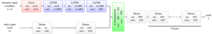
Figure 1: Proposed deep neural network architecture. The Red node corresponds to a noise generation layer. Blue nodes represent Long Short-Rerm Memory (LSTM) recurrent layers. Gray nodes represent dense, fully-connected layers. The green node represents a concatenation layer, which concatenates the intermediate representations from the dynamic and static paths. Numbers below node names represent shapes of input and output tensors. For example, $x\times y$ represents a $x$ by $y$ matrix, while single numbers represent line vectors. $n$ corresponds to the crop cycle length (in months). This figure was extended from Oliveira et al., (2018).

In this section, we describe the model (Figure 1) used to solve the problem of estimating yields of the studied crops. We also describe the data sources used and the features added to the model. Our model is based on the one proposed by Oliveira et al., (2018). The model has two separate data paths (dynamic and static) that merge inside the model. The rationale behind this design decision is that, in doing so, so-called dynamic data, such as weather data, can be processed, and specialized, by different nodes than static data, such as location and soil data. More specifically, time-series data such as weather forecasts can be processed by Long Short Term Memory (lstm) (Hochreiter, Schmidhuber,, 1997, 1997) nodes, which tend to work well with time-series data, while soil data can be processed by fully-connected nodes.

Our model expands on the original model (Oliveira et al.,, 2018) by (i) adding accumulated gdd as a dynamic feature alongside weather forecasts; (ii) making the length of the dynamic features dependent on the type of crop being used by using crop calendars as input; (iii) including an additive zero-centered Gaussian noise node at the input of the dynamic data path.

Incorporating accumulated gdd as a feature may help the model better account for the influence of temperature on the crops studied. This decision is justified because different crops have different gdd values. For example, corn requires around 1600-1770^∘c gdd for achieving full-season maturity (Neild, Newman,, 1990, 1987), while soybeans require around 1300-1500^∘c gdd from planting to physiological maturity (George et al.,, 1990). In providing this feature, we expect the model to have more opportunity to learn meaningful mappings from features to predicted yield.

One potential flaw of the model proposed by Oliveira et al., (2018) is that they use the same time window length for both crops studied (namely, soybeans and corn). In doing so, they risk adding more (or less) data to the model, harming performance by making data selection harder for the model. To mitigate this problem, we incorporated domain knowledge of crop development into our model. This data comes from crop calendars, which indicate typical planting and harvesting dates for crops in a given region. In Brazil, this information is published by Companhia Nacional de Abastecimento (conab) (Mendes et al.,, 2019).

Training a model that uses weather data as a feature has an inherent challenge: if the weather data comes from observations, the model won’t be exposed to uncertainty when used with weather forecasts. Additionally, even if weather forecasts are input as points, the model will not have been exposed to uncertainty in the weather forecasts because those would be input as point estimates. Therefore, we’ve introduced a regularization layer that adds zero-centered noise to the normalized dynamic inputs of the neural network, which doubles as a random data augmentation method.

4 Experiments

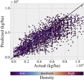
(a) Corn

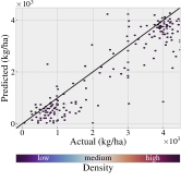
(b) Cotton

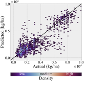
(c) Rice

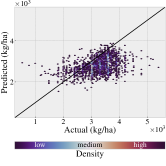
(d) Soybean

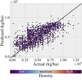
(e) Sugarcane

Figure 2: Scatter plots showing the performance of the best trained models. The vertical axis shows the predicted values, while the horizontal axis shows the actual values. All evaluation points are related to crop production in Brazil in 2018. Predictions were only performed for municipalities that actually produced the crop in the evaluation year. Points were colored differently to show densities of regions in the plots.

Crop	Train/Validation	Test
Corn	35079	5054
Cotton	1816	223
Rice	16378	1914
Soybean	14190	2315
Sugarcane	23860	3339

Table 1: Dataset sizes for each crop. Sizes were obtained after removing municipalities with zero yield. The sets were split by adding yield data related to 2018 to the Test set and the remaining data to the Train/Valitation set.

To evaluate the performance of our model, we decided to use the Produção Agrícola Municipal (pam)—Municipal Agriculture Production—dataset, a countrywide Brazilian agriculture productivity dataset, made available the Brazilian Institute of Geography and Statistics (ibge). The pam dataset concentrates data about crop production in each municipality in Brazil and makes available statistics such as area dedicated for planting, productivity in metric tonnes per hectare, average productivity, among others. Although it presents local data productivity, this information is aggregated for the municipality. Therefore, it is not possible to know exactly when and where a given crop was planted by using this dataset.

We evaluated our model using five different crops: corn, cotton, rice, soybean, and sugarcane. To do so, we downloaded the average yield data in kg/ha from the pam dataset for all municipalities in Brazil for the years 2011-2018. Since Brazil has 5435 municipalities, the dataset ended up with $5435\times 8=43480$ entries per crop. Before feeding the data into the model, we removed entries with zero productivity. Additionally, we separated the data related to the year 2018 as a test set and used it only to evaluate model performance (Table 1).

Using only the yield data is not enough to build a useful model. Hence, we augmented the pam data with weather data from the ERA5 reanalysis (Hersbach, Dee,, 2016, 2016) dataset and soil type information from the SoilGrids (Hengl et al.,, 2017) dataset, which has soil information (both observed and model-generated data) in a 250m grid for the whole planet. The weather data in question are the maximum temperature, minimum temperature, accumulated precipitation, and gdd on a monthly basis. To decide which months to gather data about, we used crop calendars provided by conab for each state-crop pair in Brazil. For example, in São Paulo state (SP), the conab document states that, for cotton, planting happens in the Spring (from October to December) while harvest happens in the Fall (April to June). Hence, we gather weather data from October to June ($n$ = 9 months) to build the dynamic input to the model. Since a municipality is defined by a polygon but we’re building a point dataset, we assume that all points in a municipality share the same features of its centroid, and we fetch data about it.

The time period in months we used for each crop are summarized in Table 2. Notice that even though we know the duration of the plant-harvest cycle, it might start at different times (and even have different lenghts) for different regions in a country and between countries. In this paper, our area of study was limited to Brazilian cities, and we used data published by conab (Companhia Nacional de Abastecimento,, 2019), summarized in Table 6. When data about a specific state was missing, we used data about the region the state belongs to.

Crop	Time period (months)
Corn	9
Cotton	9
Rice	8
Soybean	9
Sugarcane	12

Table 2: Time range of the various crops studied in this paper based on crop calendar.

With regards to the soil data, we used the seven layers of the SoilGrids dataset for nine features: clay content, silt content, sand content, bulk density, coarse fragments, cation exchange capacity, organic carbon content, pH in $H_{2}O$ and pH in $K\mathrm{Cl}$. When combined with the latitude and longitude of the centroid of the municipality, this yields the static input of the model depicted in Figure 1.

To correctly assess the performance of the model, we performed thirty independent executions of the train-test cycle. This is necessary due to the intrinsic stochasticity of the training process, which uses random initialization of the weight matrices of the neural network, as well as the random shuffling of the mini-batches in the Stochastic Gradient Descent (sgd) optimization process. For training, we used the Adam (Kingma, Ba,, 2014, 2014) algorithm with learning rate $\alpha=5\times 10^{-4}$, $\beta_{1}=0.9$, $\beta_{2}=0.999$, and a mini-batch size of 280. The maximum number of training epochs was set to 500 with early stopping set with a patience of 50. To reduce overfitting, we employed $L_{2}$ regularization, with $\lambda=1\times{}10^{-5}$.

To evaluate performance, we use two metrics: correlation and Mean Average Percent Error (mape). Correlation gives a measure of how linear the relationship between predictions and true values are, while mape measures the relative error between true values and predictions. We evaluated performance in 2018 because this is closer to how the model would be used in practice: it would be trained with all data available to make predictions for the current year. In our setting, 2018 represents this year, since it is the most recent one available in the pam dataset.

Crop	$\mu_{\text{Cor}}$	$\sigma_{\text{Cor}}$	$\mu_{\text{MAPE}}$	$\sigma_{\text{MAPE}}$
Corn	0.881	0.003	47.855	4.197
Cotton	0.924	0.003	29.238	1.516
Rice	0.874	0.004	31.484	1.194
Soybean	0.300	0.047	16.015	0.969
Sugarcane	0.710	0.012	40.877	1.656

Table 3: Model performance with noise layer in dynamic features. $\mu_{\text{Cor}}$ represents the average value of correlation metric, $\sigma_{\text{Cor}}$ represents the standard deviation of the correlation metric. Similarly, $\mu_{\text{MAPE}}$ and $\sigma_{\text{MAPE}}$ represent the average and standard deviation of the mape. Averages were computed over thirty independent executions.

Crop	$\mu_{\text{Cor}}$	$\sigma_{\text{Cor}}$	$\mu_{\text{MAPE}}$	$\sigma_{\text{MAPE}}$
Corn	0.865	0.005	51.716	6.114
Cotton	0.920	0.004	30.502	1.586
Rice	0.864	0.005	32.826	1.220
Soybean	0.288	0.025	14.755	0.565
Sugarcane	0.708	0.012	42.081	2.092

Table 4: Model performance without noise layer. $\mu_{\text{Cor}}$ represents the average value of correlation metric, $\sigma_{\text{Cor}}$ represents the standard deviation of the correlation metric. Similarly, $\mu_{\text{MAPE}}$ and $\sigma_{\text{MAPE}}$ represent the average and standard deviation of the mape. Averages were computed over thirty independent executions.

The standard deviation of the noise layer was set to 0.3, and all the input features were normalized to the 0–1 range prior to being input to the neural network. Tables 3 and 4 show the performance of the model with and without this noise layer, respectively. From the tables, it can be seen that adding a noise layer improves model performance, as correlation of the predicted yields for the model with noise layer is higher for all crops, and mape is smaller in almost all crops.

In Table 5, we show the performance of the best models found in the set of thirty for each crop. It is interesting to notice that although cotton has the smallest dataset size (Table 1), it is the one with best correlation. When we contrast this to Figure 2, which shows a scatter plot of the actual and predicted yields for 2018, we conclude correlation is a good metric, since a visual inspection indicates fit is good. For example, Figure 2b shows that there seems, indeed, to be a good fit for cotton.

We see from Tables 3 and 4 that mape for all crops is somewhat high, but upon close examination of Figure 2, one is able to see various vertical lines in all the scatter plots of crops. The vertical lines show that many municipalities have exactly the same productivity. We attribute this to the nature of the pam dataset constructed by ibge, which relies on self-reporting to compile the tables for crop production in Brazil. We believe that an increase in the precision of the data would greatly benefit the model itself and its predictions.

We also see that see that the best model for soybean (Table 5) has quite a low correlation, but low mape. Observing Figure 2d we see that soybean production seems to have low bias, but high variance. Therefore, even though correlation is low, the model makes predictions that are concentrated in the 2000–4000 kg/ha range, yielding the low mape we observe. For sugarcane, from the tables and from observing Figure 2e we see the model has good predictive power, but is probably harmed because, from the crop calendar we used, sugarcane can be planted on any month and can be harvested in any month. Due to that, the features we selected may not be powerful enough to explain the productivity, resulting is harmed performance. Therefore, even though sugarcane has the second largest dataset in this work (Table 1), the data itself is not enough to yield a good predictor.

Rice and corn have similar correlations, but different mape values. We attribute this to the model underestimating the production of large corn yields as shown in Figure 2a, which harms mape for corn. Dispersion in rice seems to be bigger in lower production values (Figure 2c), resulting in a better mape.

Crop	$\max_{\text{Cor}}$	$\min_{\text{MAPE}}$
Corn	0.886	41.596
Cotton	0.929	26.648
Rice	0.881	29.624
Soybean	0.348	13.704
Sugarcane	0.739	37.304

Table 5: Best performance of the model for each crop and metric. $\max_{\text{Cor}}$ represents the maximum correlation found over all executions for a given crop, while $\min_{\text{MAPE}}$ represents the minimum mape found over all executions for a given crop. Maximum and minimum were computed over a set of thirty independent executions.

		Planting	Harvest
State	Crop
AC	Corn	[01/10, 31/12]	[01/02, 31/05]
	Cotton	[01/12, 28/02]	[01/05, 30/06]
	Rice	[01/10, 31/12]	[01/02, 30/04]
	Soybean	[01/01, 15/06]	[01/06, 31/10]
	Sugarcane	[01/01, 31/03]	[01/04, 31/01]
AL	Corn	[01/10, 31/01]	[01/03, 30/06]
	Cotton	[01/01, 28/02]	[01/05, 30/11]
	Rice	[01/10, 31/12]	[01/01, 30/04]
	Soybean	[01/10, 28/02]	[01/03, 30/07]
	Sugarcane	[01/10, 31/08]	[01/09, 30/03]
AM	Corn	[01/04, 30/11]	[01/08, 30/04]
	Cotton	[01/12, 28/02]	[01/05, 30/06]
	Rice	[01/09, 31/12]	[01/01, 31/12]
	Soybean	[01/01, 15/06]	[01/06, 31/10]
	Sugarcane	[01/01, 31/03]	[01/04, 31/01]
AP	Corn	[01/12, 31/01]	[01/04, 31/05]
	Cotton	[01/12, 28/02]	[01/05, 30/06]
	Rice	[01/10, 31/12]	[01/02, 30/04]
	Soybean	[01/01, 15/06]	[01/06, 31/10]
	Sugarcane	[01/01, 31/03]	[01/04, 31/01]
BA	Corn	[01/10, 28/02]	[01/03, 31/08]
	Cotton	[01/11, 28/02]	[01/05, 30/09]
	Rice	[01/10, 31/01]	[01/02, 30/06]
	Soybean	[01/10, 31/01]	[01/01, 30/04]
	Sugarcane	[01/01, 31/03]	[01/04, 31/01]
CE	Corn	[01/01, 30/04]	[01/05, 31/08]
	Cotton	[01/02, 30/04]	[01/06, 31/08]
	Rice	[01/02, 30/04]	[01/05, 31/08]
	Soybean	[01/10, 28/02]	[01/03, 30/07]
	Sugarcane	[01/10, 31/08]	[01/09, 31/03]
ES	Corn	[01/10, 31/12]	[01/02, 31/05]
	Cotton	[01/11, 31/01]	[01/04, 31/07]
	Rice	[01/10, 31/12]	[01/03, 30/06]
	Soybean	[01/10, 31/12]	[01/02, 31/05]
	Sugarcane	[01/01, 31/03]	[01/04, 31/01]
GO	Corn	[01/10, 31/12]	[01/03, 30/06]
	Cotton	[01/12, 31/01]	[01/06, 31/08]
	Rice	[01/10, 31/12]	[01/03, 31/05]
	Soybean	[01/10, 31/12]	[01/01, 30/04]
	Sugarcane	[01/01, 31/03]	[01/04, 31/01]
MA	Corn	[01/11, 28/02]	[01/03, 31/08]
	Cotton	[01/12, 31/01]	[01/07, 30/09]
	Rice	[01/12, 31/03]	[01/03, 30/06]
	Soybean	[01/10, 28/02]	[01/02, 31/07]
	Sugarcane	[01/10, 31/08]	[01/09, 31/03]
MG	Corn	[01/08, 31/12]	[01/02, 30/06]
	Cotton	[01/11, 30/04]	[01/04, 30/09]
	Rice	[01/10, 31/12]	[01/03, 30/06]
	Soybean	[01/10, 31/12]	[01/01, 31/05]
	Sugarcane	[01/01, 31/03]	[01/04, 31/01]
MS	Corn	[01/09, 31/12]	[01/02, 31/05]
	Cotton	[01/10, 31/01]	[01/04, 31/08]
	Rice	[01/08, 31/12]	[01/01, 30/04]
	Soybean	[01/09, 31/12]	[01/01, 30/04]
	Sugarcane	[01/01, 31/03]	[01/04, 31/01]
MT	Corn	[01/10, 31/12]	[01/02, 30/06]
	Cotton	[01/11, 31/01]	[01/06, 30/09]
	Rice	[01/10, 31/01]	[01/01, 31/05]
	Soybean	[01/09, 31/12]	[01/01, 30/04]
	Sugarcane	[01/01, 31/03]	[01/04, 31/01]
PA	Corn	[01/10, 31/12]	[01/02, 30/06]
	Cotton	[01/12, 28/02]	[01/05, 30/06]
	Rice	[01/10, 31/12]	[01/02, 30/04]
	Soybean	[01/01, 30/04]	[01/05, 31/08]
	Sugarcane	[01/01, 31/03]	[01/04, 31/01]

		Planting	Harvest
State	Crop
PB	Corn	[01/01, 30/06]	[01/07, 31/10]
	Cotton	[01/02, 31/05]	[01/06, 31/10]
	Rice	[01/01, 31/03]	[01/05, 31/07]
	Soybean	[01/10, 28/02]	[01/03, 30/07]
	Sugarcane	[01/10, 31/08]	[01/09, 31/03]
PE	Corn	[01/01, 31/05]	[01/05, 31/08]
	Cotton	[01/01, 28/02]	[01/05, 30/11]
	Rice	[01/01, 31/03]	[01/05, 30/11]
	Soybean	[01/10, 28/02]	[01/03, 30/07]
	Sugarcane	[01/10, 31/08]	[01/09, 31/03]
PI	Corn	[01/12, 28/02]	[01/04, 31/08]
	Cotton	[01/12, 31/01]	[01/06, 31/08]
	Rice	[01/11, 28/02]	[01/03, 30/06]
	Soybean	[01/10, 31/01]	[01/02, 30/06]
	Sugarcane	[01/10, 31/08]	[01/09, 31/03]
PR	Corn	[01/09, 31/12]	[01/01, 31/05]
	Cotton	[01/01, 28/02]	[01/03, 30/06]
	Rice	[01/08, 31/12]	[01/01, 31/05]
	Soybean	[01/09, 31/12]	[01/01, 30/04]
	Sugarcane	[01/01, 31/03]	[01/04, 31/01]
RJ	Corn	[01/10, 31/12]	[01/02, 31/05]
	Cotton	[01/11, 31/01]	[01/04, 31/07]
	Rice	[01/10, 31/12]	[01/03, 30/06]
	Soybean	[01/10, 31/12]	[01/02, 31/05]
	Sugarcane	[01/01, 31/03]	[01/04, 31/01]
RN	Corn	[01/02, 31/05]	[01/06, 30/09]
	Cotton	[01/02, 30/04]	[01/06, 30/09]
	Rice	[01/03, 31/05]	[01/06, 30/11]
	Soybean	[01/10, 28/02]	[01/03, 30/07]
	Sugarcane	[01/10, 31/08]	[01/09, 31/03]
RO	Corn	[01/09, 31/12]	[01/02, 31/05]
	Cotton	[01/12, 28/02]	[01/05, 30/06]
	Rice	[01/10, 31/01]	[01/02, 30/04]
	Soybean	[01/10, 31/12]	[01/01, 30/04]
	Sugarcane	[01/01, 31/03]	[01/04, 31/01]
RR	Corn	[01/04, 31/05]	[01/09, 31/10]
	Cotton	[01/07, 30/09]	[01/02, 30/04]
	Rice	[01/04, 30/06]	[01/08, 31/10]
	Soybean	[01/04, 30/06]	[01/08, 31/10]
	Sugarcane	[01/01, 31/03]	[01/04, 31/01]
RS	Corn	[01/07, 28/02]	[01/01, 30/06]
	Cotton	[01/01, 28/02]	[01/03, 30/06]
	Rice	[01/09, 31/12]	[01/02, 31/05]
	Soybean	[01/10, 31/01]	[01/02, 31/05]
	Sugarcane	[01/01, 31/03]	[01/04, 31/01]
SC	Corn	[01/08, 31/01]	[01/01, 30/06]
	Cotton	[01/01, 28/02]	[01/03, 30/06]
	Rice	[01/08, 30/11]	[01/01, 31/05]
	Soybean	[01/10, 30/12]	[01/02, 31/05]
	Sugarcane	[01/01, 31/03]	[01/04, 31/01]
SE	Corn	[01/10, 31/01]	[01/03, 30/06]
	Cotton	[01/01, 28/02]	[01/05, 30/11]
	Rice	[01/08, 31/10]	[01/12, 28/02]
	Soybean	[01/10, 28/02]	[01/03, 30/07]
	Sugarcane	[01/10, 31/08]	[01/09, 31/03]
SP	Corn	[01/10, 31/12]	[01/03, 31/05]
	Cotton	[01/09, 31/12]	[01/04, 31/07]
	Rice	[01/09, 31/12]	[01/03, 31/05]
	Soybean	[01/09, 31/12]	[01/02, 31/05]
	Sugarcane	[01/01, 31/03]	[01/04, 31/01]
TO	Corn	[01/11, 31/01]	[01/03, 30/06]
	Cotton	[01/12, 28/02]	[01/05, 31/07]
	Rice	[01/11, 31/01]	[01/01, 31/05]
	Soybean	[01/10, 31/12]	[01/02, 31/05]
	Sugarcane	[01/01, 31/03]	[01/04, 31/01]

Table 6: Planting and harvesting dates for each state in Brazil according to the crop calendars used in this study.

5 Conclusion

This paper extended a deep-learning model from the literature (Oliveira et al.,, 2018) to support five different crops in a scalable manner. Different from previous work, which leverage satellite data for direct farm observation for yield prediction, we employ weather and soil data, which is computationally cheaper to process than large satellite images. Additionally, by using our approach one can adopt weather forecasts to predict yield before planting occurs, while using ndvi-based forecasts is only possible after plants reach a certain growth stage.

Our results show that agriculture stakeholders can get insights into potential yield even before planting to help the decision process when dealing with farm and government activities like machinery rental, contracting, price negotiation, and logistics planning. We provide accurate results even with fewer data requirements for different crops in the presence of noisy yield local data. Based on our results, it is possible to state that our model is scalable enough to provide accurate predictions to the whole world for different crops if a reliable local yield data is available.

REFERENCES

- Boogaard et al., (1998) Boogaard, H., Van Diepen, C., Rotter, R., Cabrera, J., Van Laar, H., 1998. WOFOST 7.1; user’s guide for the WOFOST 7.1 crop growth simulation model and WOFOST Control Center 1.5. Technical report, SC-DLO.
- Cai et al., (2019) Cai, Y., Guan, K., Lobell, D., Potgieter, A., Wang, S., Peng, J., Xu, T., Asseng, S., Zhang, Y., You, L., Peng, B., 2019. Integrating satellite and climate data to predict wheat yield in Australia using machine learning approaches. Agricultural and Forest Meteorology, 274, 144–159.
- Companhia Nacional de Abastecimento, (2019) Companhia Nacional de Abastecimento, 2019. Acompanhamento da Safra Brasileira. 6(4).
- DESA, Affairs, (2019) DESA, D. o. E., Affairs, S., 2019. World population prospects 2019.
- FAO, of the United Nations, (2009) FAO, F., of the United Nations, A. O., 2009. How to feed the world in 2050.
- George et al., (1990) George, T., Bartholomew, D. P., Singleton, P. W. et al., 1990. Effect of temperature and maturity group on phenology of field grown nodulating and nonnodulating soybean isolines. Biotronics, 19, 49–59.
- Hengl et al., (2017) Hengl, T., de Jesus, J. M., Heuvelink, G. B., Gonzalez, M. R., Kilibarda, M., Blagotić, A., Shangguan, W., Wright, M. N., Geng, X., Bauer-Marschallinger, B. et al., 2017. SoilGrids250m: Global gridded soil information based on machine learning. PLoS one, 12(2), e0169748.
- Hersbach, Dee, (2016) Hersbach, H., Dee, D., 2016. ERA5 reanalysis is in production. ECMWF newsletter, 147(7), 5–6.
- Hochreiter, Schmidhuber, (1997) Hochreiter, S., Schmidhuber, J., 1997. Long short-term memory. Neural computation, 9(8), 1735–1780.
- Holzworth et al., (2015) Holzworth, D. P., Snow, V., Janssen, S., Athanasiadis, I. N., Donatelli, M., Hoogenboom, G., White, J. W., Thorburn, P., 2015. Agricultural production systems modelling and software: current status and future prospects. Environmental Modelling & Software, 72, 276–286.
- Jin et al., (2018) Jin, X., Kumar, L., Li, Z., Feng, H., Xu, X., Yang, G., Wang, J., 2018. A review of data assimilation of remote sensing and crop models. European Journal of Agronomy, 92, 141–152.
- Kingma, Ba, (2014) Kingma, D. P., Ba, J., 2014. Adam: A method for stochastic optimization. arXiv preprint arXiv:1412.6980.
- Kogan et al., (2013) Kogan, F., Kussul, N., Adamenko, T., Skakun, S., Kravchenko, O., Kryvobok, O., Shelestov, A., Kolotii, A., Kussul, O., Lavrenyuk, A., 2013. Winter wheat yield forecasting in Ukraine based on Earth observation, meteorological data and biophysical models. International Journal of Applied Earth Observation and Geoinformation, 23, 192–203.
- Louhichi et al., (2010) Louhichi, K., Janssen, S., Kanellopoulos, A., Li, H., Borkowski, N., Flichman, G., Hengsdijk, H., Zander, P., Fonseca, M. B., Stokstad, G. et al., 2010. A generic farming system simulator. Environmental and Agricultural Modelling, Springer, 109–132.
- Mendes et al., (2019) Mendes, A. D., Sousa, T. D. G. F., Mendes, N. P., 2019. Calendario de Plantio e Colheira de grãos no Brasil. Technical report, Companhia Nacional de Abastecimento (Conab).
- Neild, Newman, (1990) Neild, R. E., Newman, J. E., 1990. Nch-40 growing season characteristics and requirements in the corn belt.
- Nguyen et al., (2019) Nguyen, L. H., Zhu, J., Lin, Z., Du, H., Yang, Z., Guo, W., Jin, F., 2019. Spatial-temporal multi-task learning for within-field cotton yield prediction. Q. Yang, Z.-H. Zhou, Z. Gong, M.-L. Zhang, S.-J. Huang (eds), Advances in Knowledge Discovery and Data Mining, Springer International Publishing, Cham, 343–354.
- Oliveira et al., (2018) Oliveira, I., Cunha, R. L. F., Silva, B., Netto, M. A. S., 2018. A scalable machine learning system for pre-season agriculture yield forecast. 2018 IEEE 14th International Conference on e-Science (e-Science), 423–430.
- Wang et al., (2018) Wang, A. X., Tran, C., Desai, N., Lobell, D., Ermon, S., 2018. Deep transfer learning for crop yield prediction with remote sensing data. Proceedings of the 1st ACM SIGCAS Conference on Computing and Sustainable Societies, ACM, 50.
- You et al., (2017) You, J., Li, X., Low, M., Lobell, D., Ermon, S., 2017. Deep gaussian process for crop yield prediction based on remote sensing data. AAAI, 4559–4566.