Effective resistances of two dimensional resistor networks

Abstract

We investigate the behavior of two dimensional resistor networks, with finite sizes and different kinds (rectangular, hexagonal, and triangular) of lattice geometry. We construct the network by having a network-element repeat itself $L_{x}$ times in $x$-direction and $L_{y}$ times in the $y$-direction. We study the relationship between the effective resistance ($R_{\text{eff}}$) of the network on dimensions $L_{x}$ and $L_{y}$. The behavior is simple and intuitive for a network with rectangular geometry, however, it becomes non-trivial for other geometries which are solved numerically. We find that $R_{\text{eff}}$ depends on the ratio $L_{x}/L_{y}$ in all the three studied networks. We also check the consistency of our numerical results experimentally for small network sizes.

Keywords: Circuit analysis, resistor network, electrical experiment, Kirchhoff’s laws

1 Introduction

Resistor network problems have been widely studied in various contexts, starting from textbook physics and competitive tests [1] to electrical engineering [2], condensed matter physics [3], and statistical physics [4]. Since many regular electrical networks take shapes of meshes, similar to the lattices in solid state crystals, it is intriguing to find out the equivalent or effective resistance of such networks. There had been extensive studies on two-dimensional lattices in order to investigate percolation based conductivity [5] in such systems and methods like effective medium theory [5, 6, 7, 8] and Green’s function method [5, 9, 10, 11] have been formulated. However, most of these studies focus on the infinite systems with stochastic resistance distribution (random resistor network). Although a few studies have been conducted recently for finite size networks, such studies either investigated equivalent resistance between two points inside the network or for networks that do not obey the typical crystal lattice symmetries [12, 13, 14, 11, 15, 16]. Hence dimensional dependence of effective resistance ($R_{\text{eff}}$) for various geometries deserves separate attention and it also bears an academic interest to show how $R_{\text{eff}}$ can simply be estimated by solving a set of electrical equations. Network geometry dependence of $R_{\text{eff}}$ brings the connection to the graph theory [17, 18] and generalization of $Y$-$\Delta$ or star-polygon transformation can open doors of future research [19]. The networks described in our paper are very straightforward and easy to solve numerically once the correct equations are formulated. However, such solutions do not exist in the literature to the best of our knowledge and hence our findings are both pedagogical and research oriented. Given resources, the network models can be constructed by students easily and knowing the dependence of $R_{\text{eff}}$ on the geometry, a device can be designed whose resistance can be controlled by tuning its dimensions.

Our paper is organized in the following way. We first explain the generic resistor network setup and then discuss the analytical solution for the rectangular geometry. Then we discuss the numerical formulation and $R_{\text{eff}}$’s dependence on the dimensions, obtained from our numerical results for rectangular, hexagonal, and triangular resistor networks. As a summary, we compare these results for these three different geometries and finally we describe a small experiment to test our theoretical findings.

2 Generic resistor network configuration

We describe below our generic setup for various lattice geometries:

1. Define a two dimensional (2D) lattice. Though the geometry varies lattice to lattice, we define the size of each lattice by two Cartesian lengths $L_{x}$ and $L_{y}$. For a rectangular lattice, $L_{x}L_{y}$ becomes the number of the lattice points or sites as well.

2. Each lattice point attaches to a resistance of value $R$ spreading along the direction of its neighborhood lattice points.

3. Apply a bias $V$ at one edge of the lattice (say in the direction of the length $L_{x}$) and ground the other edge (hence the lattice acts like an active medium attached to a battery or applied voltage). Only one point from each unit cell of the lattice is attached to the bias or grounding and such points must be equivalent for all unit cells of the lattice.

Typically, electrical networks with resistors and biases are solved by using one of the Kirchhoff’s laws of circuit (originally announced by Gustav Kirchhoff in 1845) [20, 21], which is often termed as mesh-current or nodal analysis by electrical engineers [2]. Out of Kirchhoff’s voltage and current laws, it is more convenient to use the current law that states that total current at a circuit junction (lattice point or site in our case) must be zero. Hence the key equation for the Kirchhoff’s current law (KCL) at a site or node $(i,j)$ in 2D Cartesian coordinate:

$$\sum_{k}I_{ij}(k)=0\Rightarrow\sum_{k}[(V_{ik}-V_{ij})/R_{ik}+(V_{kj}-V_{ij})/R_{jk}]=0\,$$ (1)

where $k$ denotes all nearest neighbor nodes (lattice points, voltage or grounding connection) to the site $(i,j)$. We discuss the implementation of this in the forthcoming sections, where we formulate them in the form of a matrix equation for various network geometries.

3 Rectangular resistor network

As the most common 2D geometry, we begin with a finite size rectangular lattice defined by lengths $L_{x}$ and $L_{y}$. Following the setup defined in the previous section, a voltage $V$ is applied at one end of the lattice, in the direction of the length $L_{x}$ (see  Fig. 1) while the other end is grounded. Resistances, each with value $R$, are connected to each site in all four directions. Our objective is to find out the effective resistance ($R_{\text{eff}}$) for the geometry and how $R_{\text{eff}}$ depends on the dimensions $L_{x}$ and $L_{y}$.

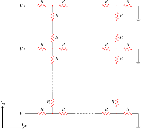
Fig. 1: A resistor network on a rectangular lattice geometry.

3.1 Analytical solution:

To find out the effective resistance in the lattice, for a moment, we assume there are no resistive connections in the $y$ (vertical) direction. Thus for a lattice of size $L_{x}\times L_{y}$, points are connected only in the $x$-direction (see  Fig. 2). There are total $L_{y}$ branches of parallel resistances with each branch consisting of a set of resistances in series. Now in each set of resistances in series, we can notice that the equivalent resistance between two adjacent sites is $R+R=2R$ (resistance $R$ on the left of one site and on the right of the other site). Thus we find $L_{x}-1$ number of resistances of value $2R$ between first and last lattice points and two resistances of value $R$ on the left and right ends of the lattice. Thus in total, we have $L_{x}$ number of resistances of value $2R$ in series on each branch. Thus equivalent resistance of each branch is $2RL_{x}$. Since there exist $L_{y}$ such branches in parallel, the overall effective resistance of this simplified circuit:

$$R_{\text{eff}}^{\text{simp}}=\big{[}1/(2RL_{x})+\cdots\mbox{($L_{y}$ times)}\big{]}{{}^{-1}}=2RL_{x}/L_{y}\,.$$ (2)

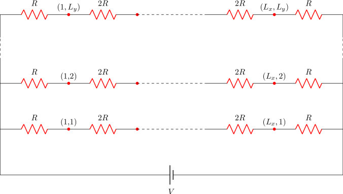
Fig. 2: A network of resistors connected only in the $x$-direction.

Fig. 3: (a) Two resistances in series. (b) A simple Wheatstone bridge, which is a realization of the case $L_{x}=1$, $L_{y}=2$ in the rectangular network.

We know that when two resistances ($R_{1}$ and $R_{2}$) are connected in series, as shown in  Fig. 3, the potential drop after the first resistance $R_{1}$ (i.e. in the middle of $R_{1}$ and $R_{2}$) will be given by

$$V-V_{1}=V\frac{R_{1}}{R_{1}+R_{2}}\,,$$ (3)

which gives the potential at the middle of $R_{1}$ and $R_{2}$:

$$V_{1}=V\bigg{(}1+\frac{R_{1}}{R_{1}+R_{2}}\bigg{)}\,.$$ (4)

Extending this argument to our case, the potential at a point $(i,j)$ will be

$$V_{i,j}=V\,\bigg{(}1+\frac{2iR}{2RL_{x}}\bigg{)}=V\,\bigg{(}1+\frac{i}{L_{x}}\bigg{)}\,.$$ (5)

since there are equivalent resistance of value $(i-1).2R+R=2iR$ [$(i-1)$ resistances with value $2R$ plus a single resistance with value $R$] resistances to the left of point $(i,j)$. Eq. (5) shows that the potential at any branch is independent of $y$-coordinate.

Thus, even if we were to connect the points in the $y$-direction using resistances of the same value (which was our original network to begin with), no current would flow in the $y$-direction for the same $x$-coordinate. This means that the original network, with all the lattice points joined, is equivalent to the network with lattice points joined only in the $x$-direction. Since the two networks are equivalent, the effective resistances of the original rectangular network will be the same as the one in Eq. (2):

$$R_{\text{eff}}^{\text{rect}}=2R\,\frac{L_{x}}{L_{y}}=R\frac{z}{2}\frac{L_{x}}{L_{y}}\,$$ (6)

where we attempt to write the formula in a more generic form by looking at the coordination number $z$ (number of nearest neighbor sites, $z=4$ for a rectangular lattice). We can easily notice that a balanced Wheatstone bridge [2] with resistance $R$ on each of its branches is the $L_{x}=1$ and $L_{y}=2$ case of the rectangular network (see Fig. 3). There, by applying Eq. (6), we get $R_{\text{eff}}=2R.1/2=R$ which is supposed to be the desired result for the bridge network.

3.2 Numerical Formulation:

In our rectangular lattice of size $L_{x}\times L_{y}$, we can mark out distinct 9 kinds of lattice points:

• Left bottom corner point ($i=1$, $j=1$)

• Left top corner point ($i=1$, $j=L_{y}$)

• Right bottom corner point ($i=L_{x}$, $j=1$)

• Right top corner point ($i=L_{x}$, $j=L_{y}$)

• Left Non-corner edge points ($i=1$, $j\in[2,L_{y}-1]$)

• Bottom non-corner edge points ($i\in[2,L_{x}-1]$, $j=1$)

• Right non-corner edge points ($i=L_{x}$, $j\in[2,L_{y}-1]$)

• Top non-corner edge points ($j=L_{y}$, $i\in[2,L_{x}-1]$)

• Non-border inner points ($i\in[2,L_{x}-1]$, $j\in[2,L_{y}-1]$)

The KCLs for the above 9 kinds of points follow:

1. Left bottom corner point $\rightarrow$ $i=1$, $j=1$:

   $$\frac{V−V_{1,1}}{R}+\frac{V_{2,1}−V_{1,1}}{2R}+\frac{V_{1,2}−V_{1,1}}{2R}=0\,.$$ (7)

2. Left top corner point $\rightarrow$ $i=1$, $j=L_{y}$:

   $$\frac{V−V_{1,Ly}}{R}+\frac{V_{2,Ly}−V_{1,Ly}}{2R}+\frac{V_{1,Ly−1}−V_{1,Ly}}{2R}=0\,.$$ (8)

3. Right bottom corner point $\rightarrow$ $i=L_{x}$, $j=1$:

   $$\frac{V_{Lx−1,1}−V_{Lx,1}}{2R}-\frac{V_{Lx,1}}{R}+\frac{V_{Lx,2}−V_{Lx,1}}{2R}=0\,.$$ (9)

4. Right top corner point $\rightarrow$ $i=L_{x}$, $j=L_{y}$:

   $$\frac{V_{Lx−1,Ly}−V_{Lx,Ly}}{2R}-\frac{V_{Lx,Ly}}{R}+\frac{V_{Lx,Ly−1}−V_{Lx,Ly}}{2R}=0\,.$$ (10)

5. Left non-corner edge point $\rightarrow$ $i=1$, $j=2$ to $L_{y}−1$:

   $$\frac{V−V_{1,j}}{R}+\frac{V_{2,j}−V_{1,j}}{2R}+\frac{V_{1,j−1}−V_{1,j}}{2R}+\frac{V_{1,j+1}−V_{1,j}}{2R}=0\,.$$ (11)

6. Right non-corner edge point $\rightarrow$ $i=L_{x}$, $j=2$ to $L_{y}−1$:

   $$\frac{V_{Lx−1,j}−V_{Lx,j}}{2R}-\frac{V_{Lx,j}}{R}+\frac{V_{Lx,j−1}−V_{Lx,j}}{2R}+\frac{V_{Lx,j+1}−V_{Lx,j}}{2R}=0\,.$$ (12)

7. Bottom non-corner edge point $\rightarrow$ $i=2$ to $L_{x}$, $j=1$:

   $$\frac{V_{i−1,1}−V_{i,1}}{2R}+\frac{V_{i+1,1}−V_{i,1}}{2R}+\frac{V_{i,2}−V_{i,1}}{2R}=0\,.$$ (13)

8. Top non-corner edge point $\rightarrow$ $i=2$ to $L_{x}$, $j=L_{y}$:

   $$\frac{V_{i−1,Ly}−V_{i,Ly}}{2R}+\frac{V_{i+1,1}−V_{i,Ly}}{2R}+\frac{V_{i,Ly−1}−V_{i,Ly}}{2R}=0\,.$$ (14)

9. Non-border inner point $\rightarrow$ $i=2$ to $L_{x}−1$, $j=2$ to $L_{y}−1$:

   $$\frac{V_{i−1,j}−V_{i,j}}{2R}+\frac{V_{i+1,j}−V_{i,j}}{2R}+\frac{V_{i,j−1}−V_{i,j}}{2R}+\frac{V_{i,j+1}−V_{i,j}}{2R}=0\,.$$ (15)

We can rearrange the above equations by collecting the coefficients of $V_{ij}$:

1. Left bottom corner point $\rightarrow$ $i=1$, $j=1$:

   $$\bigg{[}\frac{1}{R}+\frac{1}{2R}+\frac{1}{2R}\bigg{]}V_{1,1}-\frac{1}{2R}V_{2,1}-\frac{1}{2R}V_{1,2}=\frac{V}{R}\,.$$ (16)

2. Left top corner point $\rightarrow$ $i=1$, $j=L_{y}$:

   $$\bigg{[}\frac{1}{R}+\frac{1}{2R}+\frac{1}{2R}\bigg{]}V_{1,L_{y}}-\frac{1}{2R}V_{2,L_{y}}-\frac{1}{2R}V_{1,L_{y}-1}=\frac{V}{R}\,.$$ (17)

3. Right bottom corner point $\rightarrow$ $i=L_{x}$, $j=1$:

   $$\bigg{[} \frac{1}{2R}+\frac{1}{R}+\frac{1}{2R}\bigg{]}V_{L_{x},1}-\frac{1}{2R}V_{L_{x}-1,1}-\frac{1}{2R}V_{L_{x},2}=0\,.$$ (18)

4. Right top corner point $\rightarrow$ $i=L_{x}$, $j=L_{y}$:

   $$\bigg{[}\frac{1}{2R}+\frac{1}{R}+\frac{1}{2R}\bigg{]}V_{L_{x},L_{y}}-\frac{1}{2R}V_{L_{x}-1,L_{y}}-\frac{1}{2R}V_{L_{x},L_{y}-1}=0\,.$$ (19)

5. Left non-corner edge point $\rightarrow$ $i=1$, $j=2$ to $L_{y}-1$:

   $$\bigg{[}\frac{1}{R}+\frac{1}{2R}+\frac{1}{2R}+\frac{1}{2R}\bigg{]}V_{1,j}-\frac{1}{2R}V_{2,j}-\frac{1}{2R}V_{1,j-1}-\frac{1}{2R}V_{1,j+1}=\frac{V}{R}\,.$$ (20)

6. Right non-corner edge point $\rightarrow$ $i=L_{x}$, $j=2$ to $L_{y}-1$:

   $$\bigg{[}\frac{1}{2R}+\frac{1}{R}+\frac{1}{2R}+\frac{1}{2R}\bigg{]}V_{L_{x},j}-\frac{1}{2R}V_{L_{x}-1,j}-\frac{1}{2R}V_{L_{x},j-1}-\frac{1}{2R}V_{L_{x},j+1}=0\,.$$ (21)

7. Bottom non-corner edge point $\rightarrow$ $i=2$ to $L_{x}$, $j=1$:

   $$\bigg{[}\frac{1}{2R}+\frac{1}{2R}+\frac{1}{2R}\bigg{]}V_{i,1}-\frac{1}{2R}V_{i-1,1}-\frac{1}{2R}V_{i+1,1}-\frac{1}{2R}V_{i,2}=0\,.$$ (22)

8. Top non-corner edge point $\rightarrow$ $i=2$ to $L_{x}$, $j=L_{y}$:

   $$\bigg{[}\frac{1}{2R}+\frac{1}{2R}+\frac{1}{2R}\bigg{]}V_{i,L_{y}}-\frac{1}{2R}V_{i-1,L_{y}}-\frac{1}{2R}V_{i+1,1}-\frac{1}{2R}V_{i,L_{y}-1}=0\,.$$ (23)

9. Non-border inner point $\rightarrow$ $i=2$ to $L_{x}-1$, $j=2$ to $L_{y}-1$:

   $$\bigg{[} \frac{1}{2R}+\frac{1}{2R}+\frac{1}{2R}+\frac{1}{2R}\bigg{]}V_{i,j}-\frac{1}{2R}V_{i-1,j}-\frac{1}{2R}V_{i+1,j}-\frac{1}{2R}V_{i,j-1}-\frac{1}{2R}V_{i,j+1}=0\,.$$ (24)

Now $V_{ij}$’s constitute a $L_{x}\times L_{y}$ matrix, but if we linearize (see Appendix for details) it as a column vector $\bf V$ of length $L_{x}L_{y}$, The above equations can be represented in matrix notation as

$${\bf GV=I}$$ (25)

where $\bf I$ is a column vector whose values are given by the right hand side of equations $(7)$ to $(15)$ and G is a matrix consisting of the coefficients of the variables in the equations. Since G has units $1/R$, we are calling it the conductance matrix. Since the potential at any lattice point $(i,j)$ depends only on its neighboring points, the matrix G is generally sparse, and can be solved using a sparse matrix solver numerically. The method is very similar to typical transfer matrix method used in circuit analysis [22] and also similar to the method used in the context of disordered resistor network [23].

Once the above matrix system is solved and we know the potential at all lattice points, the effective resistance can be determined by dividing the total applied voltage by net current flowing through the lattice in the direction of the applied voltage. It can be observed that the net current can be determined using the potential of the end-points of the lattice. The net current, in this case, would be given by

$$I_{\text{net}}=\frac{\Sigma^{L_{y}}_{j=1}V_{Lx,j}}{R}\,.$$ (26)

Effective Resistance can then be determined as

$$R_{\text{eff}}=\frac{V}{I_{\text{net}}}\,.$$ (27)

In practice, we choose $R=1$ and $V=1$.

3.3 Results:

We first plot $R_{\text{eff}}$ against $L_{x}$ for several fixed values of $L_{y}$. As expected from the analytical solution expressed in Eq. (6), $R_{\text{eff}}$ grows linearly as $L_{x}$ increases and the slope of the linear curve drops at a larger value of $L_{y}$ (see Fig. 4).

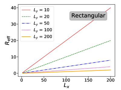
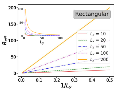
Fig. 4: A plot of $R_{\text{eff}}$ as (a) $L_{x}$ is varied for different values of $L_{y}$ and (b) $L_{y}$ is varied for different values of $L_{x}$ for a rectangular lattice.

When $L_{x}$ is kept constant, $R_{\text{eff}}$ decreases as $L_{y}$ increases and $R_{\text{eff}}$ vs $1/L_{y}$ plots show linear, establishing that $R_{\text{eff}}\propto L_{x}/L_{y}$. Now to find out the proportionality constant, we define

$$r\equiv\frac{R_{\text{eff}}L_{y}}{RL_{x}}$$ (28)

which according to Eq. (6) should be equal to $z/2=2$. Both Fig. 5 and Fig. 5 show that $r$ is a constant when $L_{x}$ and $L_{y}$ are varied respectively, keeping the other dimension as a fixed parameter. The value of the constant is 2 and hence we see that the numerical results very well agree with our analytical formula.

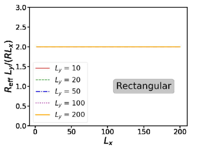
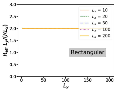
Fig. 5: A plot of $r=R_{\text{eff}}L_{y}/(RL_{x})$ as (a) $L_{x}$ and (b) $L_{y}$ is varied while other parameters are kept fixed. Both show $R_{\text{ratio}}=2$ and it is independent of dimensions $L_{x}$ and $L_{y}$.

4 Hexagonal Network Model

Now we consider the hexagonal or the graphene [24] type honeycomb lattice network. Out of two possible orientations, we select a hexagonal lattice which has armchair edges in the $x$-direction and zigzag edges in the $y$-direction (see Fig. 6) and dub this armchair hexagonal lattice.

4.1 Numerical formulation:

Here for our convenience, we break the sites into two categories – (i) $M$-type sites, sitting at the middle corners of a hexagon and such sites connect to the bias and grounding, and (ii) $S$-type sites, sitting on the top or bottom sides of a hexagon. We add extra indices 0 and 1 to specify $M$ and $S$ sites respectively. Now we can see there must be always equal and even numbers of $M$ and $S$ sites in the $x$-direction in a lattice with complete hexagons. The number of $M$ and $S$ sites ($L_{M}$ or $L_{S}$) sets the measurement of the length $L_{x}$: $L_{x}=L_{x}^{M}=L_{x}^{S}$. On the other hand, the number of voltage connection determines the length $L_{y}$: $L_{y}=L_{y}^{M}$, $L_{y}^{S}=L_{y}^{M}+1=L_{y}+1$. Total number of sites can be determined as $N_{\text{site}}=L_{x}^{M}L_{y}^{M}+L_{x}^{S}L_{y}^{S}=L_{x}L_{y}+L_{x}(L_{y}+1)=L_{x}(2L_{y}+1)$. We can distinguish 6 kinds of sites in this system:

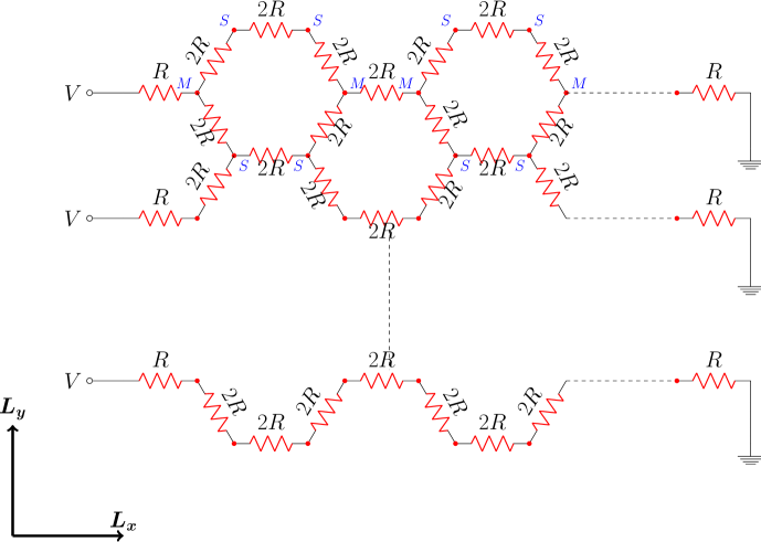
Fig. 6: A resistor network on a hexagonal lattice geometry.

• Left Border Points ($i=1$, $j=1$ to $L_{y}$, $k=0$)

• Right Border Points ($i=L_{x}$, $j=1$ to $L_{y}$, $k=0$)

• Top border points ($i=1$ to $L_{x},j=L_{y}+1,k=1$)

• Bottom Border Points ($i=1$ to $L_{x}$, $j=1$, $k=1$)

• $M$-type inner points ($i=2$ to $L_{x}-1$, $j=1$ to $L_{y}$, $k=0$)

• $S$-type inner points ($i=1$ to $L_{x}$, $j=2$ to $L_{y}$, $k=1$)

The KCL for the above 6 kinds of points would be:

1. Left Border Points $\rightarrow$ $i=1$, $j=1$ to $L_{y}$, $k=0$:

   $$\frac{V-V_{1,j,0}}{R}+\frac{V_{1,j,1}-V_{1,j,0}}{2R}+\frac{V_{1,j+1,1}-V_{1,j,0}}{2R}=0\,.$$ (29)

2. Right Border Points $\rightarrow$ $i=L_{x}$, $j=1$ to $L_{y}$, $k=0$:

   $$\frac{-V_{2Lx,j,0}}{R}+\frac{V_{2Lx,j,1}-V_{2Lx,j,0}}{2R}+\frac{V_{2Lx,j+1,1}-V_{2Lx,j,0}}{2R}=0\,.$$ (30)

3. Top Border Points $\rightarrow$ $i=1$ to $L_{x}$, $j=L_{y}+1$, $k=1$:
   if i=odd,

   $$\frac{V_{i,Ly,0}-V_{i,Ly+1,1}}{2R}+\frac{V_{i+1,Ly+1,1}-V_{i,Ly+1,1}}{2R}=0\,.$$ (31)

   if i=even,

   $$\frac{V_{i,Ly,0}-V_{i,Ly+1,1}}{2R}+\frac{V_{i-1,Ly+1,1}-V_{i,Ly+1,1}}{2R}=0\,.$$ (32)

4. Bottom Border Points $\rightarrow$ $i=1$ to $L_{x}$, $j=1$, $k=1$:
   if i=odd,

   $$\frac{V_{i,1,0}-V_{i,1,1}}{2R}+\frac{V_{i+1,1,1}-V_{i,1,1}}{2R}=0\,.$$ (33)

   if i=even,

   $$\frac{V_{i,1,0}-V_{i,1,1}}{2R}+\frac{V_{i-1,1,1}-V_{i,1,1}}{2R}=0\,.$$ (34)

5. $M$-type inner points $\rightarrow$ $i=2$ to $L_{x}-1$, $j=1$ to $L_{y}$, $k=0$:
   if i=odd,

   $$\frac{V_{i-1,j,0}-V_{i,j,0}}{2R}+\frac{V_{i,j,1}-V_{i,j,0}}{2R}+\frac{V_{i,j+1,1}-V_{i,j,0}}{2R}=0\,.$$ (35)

   if i=even,

   $$\frac{V_{i+1,j,0}-V_{i,j,0}}{2R}+\frac{V_{i,j,1}-V_{i,j,0}}{2R}+\frac{V_{i,j+1,1}-V_{i,j,0}}{2R}=0\,.$$ (36)

6. $S$-type inner points $\rightarrow$ $i=1$ to $L_{x}$, $j=2$ to $L_{y}$, $k=1$:
   if i=odd,

   $$\frac{V_{i+1,j,1}-V_{i,j,1}}{2R}+\frac{V_{i,j,0}-V_{i,j,1}}{2R}+\frac{V_{i,j-1,0}-V_{i,j,1}}{2R}=0\,.$$ (37)

   if i=even,

   $$\frac{V_{i-1,j,1}-V_{i,j,1}}{2R}+\frac{V_{i,j,0}-V_{i,j,1}}{2R}+\frac{V_{i,j-1,0}-V_{i,j,1}}{2R}=0\,.$$ (38)

Note that here we have two types of sites, namely $M$ and $S$, and that though we use $(i,j)$ to denote the two-dimensional location different types of sites, a particular kind of site belongs to a particular type and hence one type’s $i$ or $j$ should not coincide with another type’s $i$ or $j$ and this distinction is taken care by the index $k$. As before, the above equations can be represented in matrix notation and are solved using a sparse matrix solver.

4.2 Results:

Like in the previous case, we first plot $R_{\text{eff}}$ as $L_{x}$ is varied, keeping $L_{y}$ fixed at different values. Even for a hexagonal lattice, $R_{\text{eff}}$ seems to increase linearly with $L_{x}$, as seen in Fig. 7. We then plot $R_{\text{eff}}$ as $L_{y}$ is varied, keeping $L_{x}$ fixed at different values. The result is shown in Fig. 7. Though $R_{\text{eff}}$ decreases with increasing $L_{y}$ like in the rectangular lattice case, $R_{\text{eff}}$ vs $1/L_{y}$ plots are not exactly linear (see  Fig. 7).

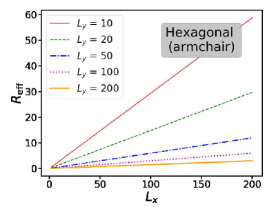
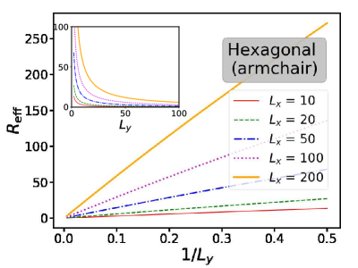
Fig. 7: Plot of $R_{\text{eff}}$ as (a) $L_{x}$ is varied for different values of $L_{y}$ and (b) $L_{y}$ is varied for different values of $L_{x}$ for an armchair hexagonal lattice based network.

To see what is the actual dependence, we again plot the ratio $r=R_{\text{eff}}L_{y}/(RL_{x})$ against $L_{x}$ and $L_{y}$ keeping other parameters fixed. We found a few interesting observations: (i) When $L_{y}$ is fixed, the ratio $r$ becomes independent of $L_{x}$; (ii) When $L_{x}$ is fixed, $r$ becomes universal and it approaches a constant at the thermodynamic limit ($L_{y}\to\infty$). These two observations, as shown in Fig. 8, let us arrive at a conclusion that the ratio is a sole function of $L_{y}$:

$$r=\alpha(L_{y})\,.$$ (39)

This leads to an empirical formula for the effective resistance:

$$R_{\text{eff}}^{\text{hex}}=\alpha(L_{y})\frac{L_{x}}{L_{y}}\,.$$ (40)

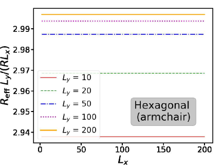
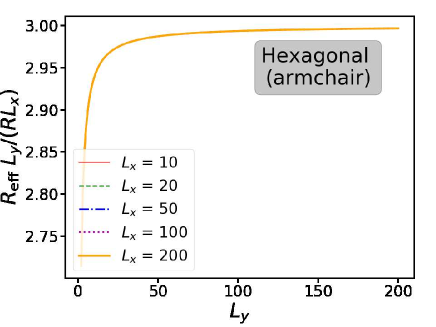
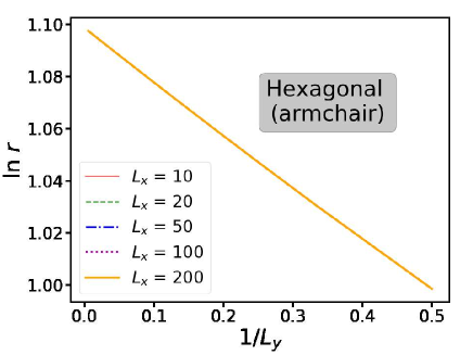
Fig. 8: Plot of $r=R_{\text{eff}}L_{y}/(R\L_{x})$ as (a) $L_{y}$ is varied for different values of $L_{x}$ and (b) as $L_{x}$ is varied for different values of $L_{y}$ for an armchair hexagonal lattice. (c) $\ln r$ plotted against $1/L_{y}$ to verify the formula given in Eq. (41) for $\alpha$ where $r=\alpha(z,L_{y})$.

Now we further notice that $\alpha(z,L_{y})$ approaches $z$ as $L_{y}\to\infty$ where $z=3$ is the lattice coordination number for a hexagonal lattice. Since $\alpha(z,L_{y})$ has to be dimensionless to keep Eq. (39) physically consistent, a convenient guess could be

$$\alpha(L_{y})=z\,e^{-c/L_{y}}\,$$ (41)

which implies

$$\ln\alpha(L_{y})=\ln z-cL_{y}{{}^{-1}}\,.$$ (42)

where $c$ is a constant. Now Fig. 8 plots $\ln\alpha$ against $L_{y}{{}^{-1}}$ for various $L_{x}$ and we can see when $L_{y}{{}^{-1}}$ approaches zero (thermodynamic limit), $\ln\alpha$ approaches $\ln z=\ln 3\simeq 1.1$ vindicating our guessed formula for $\alpha$ in Eq. (41).

5 Triangular Network Model

We now move to the case where the lattice is triangular. The network considered is shown in Fig. 9. Clearly this lattice is similar to a rectangular lattice, with the exception that diagonal points in one particular direction are also connected via an equivalent resistance $2R$.

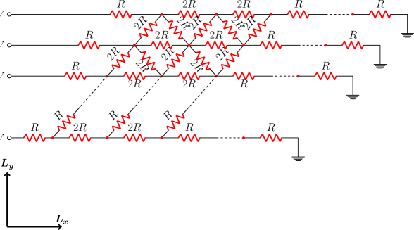
Fig. 9: A resistor network on a triangular lattice geometry.

5.1 Numerical formulation:

For a triangular lattice, we have 9 kinds of lattice points:

• Left bottom corner point $(i=1,j=1)$

• Left top corner point $(i=1,j=L_{y})$

• Right bottom corner point $(j=1,i=L_{x})$

• Right top corner point $(i=L_{x},j=L_{y})$

• Left non-corner edge points $(i=1,j\in[2,L_{y}-1])$

• Right non-corner edge points $(i=L_{x},j\in[2,L_{y}-1])$

• Bottom non-corner edge points $(j=1,in\in[2,L_{x}-1])$

• Top non-corner edge points $(j=L_{y},i\in[2,L_{x}-1])$

• Non-border inner points $(i\in[2,L_{x}-1],j\in[2,L_{y}-1])$)

The KCL, that relates the potential at any point $(i,j)$ with its neighboring point, for the above 9 kinds of points would be as follows:

1. Left bottom corner point $\rightarrow$ $i=1$, $j=1$:

   $$\frac{V−V_{1,1}}{R}+\frac{V_{2,1}−V_{1,1}}{2R}+\frac{V_{1,2}−V_{1,1}}{2R}=0\,.$$ (43)

2. Left top corner point $\rightarrow$ $i=1$, $j=L_{y}$:

   $$\frac{V−V_{1,Ly}}{R}+\frac{V_{2,Ly}−V_{1,Ly}}{2R}+\frac{V_{1,Ly−1}−V_{1,Ly}}{2R}+\frac{V_{2,Ly−1}−V_{1,Ly}}{2R}=0\,.$$ (44)

3. Right bottom corner point $\rightarrow$ $i=L_{x}$, $j=1$:

   $$\frac{V_{Lx−1,1}−V_{Lx,1}}{2R}-\frac{V_{Lx,1}}{R}+\frac{V_{Lx,2}−V_{Lx,1}}{2R}+\frac{V_{Lx-1,2}−V_{Lx,1}}{2R}=0\,.$$ (45)

4. Right top corner point $\rightarrow$ $i=L_{x}$, $j=L_{y}$:

   $$\frac{V_{Lx−1,Ly}−V_{Lx,Ly}}{2R}-\frac{V_{Lx,Ly}}{R}+\frac{V_{Lx,Ly−1}−V_{Lx,Ly}}{2R}=0\,.$$ (46)

5. Left non-corner edge point $\rightarrow$ $i=1$, $j=2$ to $L_{y}−1$:

   $$\frac{V−V_{1,j}}{R}+\frac{V_{2,j}−V_{1,j}}{2R}+\frac{V_{1,j−1}−V_{1,j}}{2R}+\frac{V_{1,j+1}−V_{1,j}}{2R}+\frac{V_{2,j-1}-V_{1,j}}{2R}=0\,.$$ (47)

6. Right non-corner edge point $\rightarrow$ $i=L_{x}$, $j=2$ to $L_{y}−1$:

   $$\frac{V_{Lx−1,j}−V_{Lx,j}}{2R}-\frac{V_{Lx,j}}{R}+\frac{V_{Lx,j−1}−V_{Lx,j}}{2R}+\frac{V_{Lx,j+1}−V_{Lx,j}}{2R}+\frac{V_{Lx-1,j+1}−V_{Lx,j}}{2R}=0\,.$$ (48)

7. Bottom non-corner edge point $\rightarrow$ $i=2$ to $L_{x}$, $j=1$:

   $$\frac{V_{i−1,1}−V_{i,1}}{2R}+\frac{V_{i+1,1}−V_{i,1}}{2R}+\frac{V_{i,2}−V_{i,1}}{2R}+\frac{V_{i-1,2}−V_{i,1}}{2R}=0\,.$$ (49)

8. Top non-corner edge point $\rightarrow$ $i=2$ to $L_{x}$, $j=L_{y}$:

   $$\frac{V_{i−1,Ly}−V_{i,Ly}}{2R}+\frac{V_{i+1,1}−V_{i,Ly}}{2R}+\frac{V_{i,Ly−1}−V_{i,Ly}}{2R}+\frac{V_{i+1,Ly−1}−V_{i,Ly}}{2R}=0\,.$$ (50)

9. Non-border inner point $\rightarrow$ $i=2$ to $L_{x}−1$, $j=2$ to $L_{y}−1$:

   $$\frac{V_{i−1,j}−V_{i,j}}{2R}+\frac{V_{i+1,j}−V_{i,j}}{2R}+\frac{V_{i,j−1}−V_{i,j}}{2R}+\frac{V_{i,j+1}−V_{i,j}}{2R}+\frac{V_{i-1,j+1}−V_{i,j}}{2R}+\frac{V_{i+1,j-1}−V_{i,j}}{2R}=0\,.$$ (51)

5.2 Results:

After solving the above equations in the matrix form, we plot $R_{\text{eff}}$ against $L_{x}$ keeping $L_{y}$ fixed at various values. We again notice that $R_{\text{eff}}$ increases with $L_{x}$ and $1/L_{y}$ (see Fig. 10). However, unlike the rectangular or hexagonal lattice network, the dependence of $R_{\text{eff}}$ is not strictly linear, rather it only becomes linear in $L_{x}$ at large value of $L_{x}$ or $L_{y}$ (see Fig. 10).

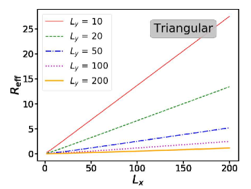
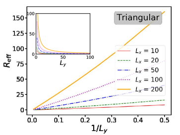
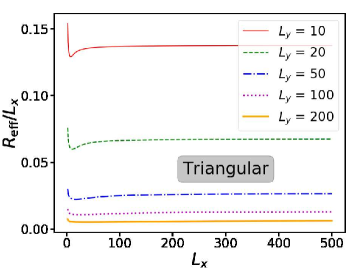
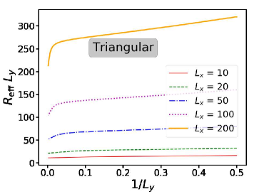
Fig. 10: Plot of $R_{\text{eff}}$ against (a) $L_{x}$ for different values of $L_{x}$ and (b) $1/L_{y}$ (inset: against $L_{y}$) for different values of $L_{x}$ for a triangular lattice. (c) $R_{\text{eff}}/L_{x}$ vs $L_{x}$ plots show that $R_{\text{eff}}$ depends linearly on $L_{x}$ only at large $L_{x}$ or $L_{y}$. (d) $R_{\text{eff}}/L_{y}$ vs $L_{y}$ plots show that $R_{\text{eff}}$ does not strictly depends linearly on $1/L_{y}$.

Now we look at the ratio $r=R_{\text{eff}}L_{y}/(RL_{x})$ and find that it depends non-trivially on both $L_{x}$ and $L_{y}$. As can be noticed from Fig. 11 and Fig. 11, $r$ approaches a constant value only when $L_{x}/L_{y}$ (when $L_{x}$ varied, $L_{y}$ fixed) or $L_{y}/L_{x}$ (when $L_{y}$ varied, $L_{x}$ fixed) is significantly large (i.e. $L_{x}$ or $L_{y}$ approaches the thermodynamic limit compared to the other dimension). However, unlike the earlier two lattice cases, we could not trivially figure out any empirical function or formula for the $R_{\text{eff}}$’s dependence on $L_{x}$ and $L_{y}$ for the triangular lattice network. We presume that this non-triviality arises because of the diagonal resistance dependence of the circuit current which is absent in hexagonal and rectangular lattice networks. Also, one should note that hexagonal lattice is a brick-wall lattice, which is a shifted version of a rectangular lattice and hence both lattices bear a similarity in the current flow distribution, and in that sense, triangular lattice network is entirely unique. Only the natural expectation that the effective resistance will be independent of dimension at a large value of $L_{x}$ and $L_{y}$ have been reflected in all three different lattice networks discussed in our paper.

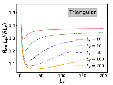
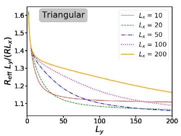
Fig. 11: Plot of $r=R_{\text{eff}}L_{y}/(RL_{x})$ vs $L_{y}$ as $L_{y}$ is varied for different values of $L_{x}$ for a triangular lattice.

6 Summary

Now in Table 1, we briefly summarize $R_{\text{eff}}$’s dependence on the dimensions for various network geometries that we discussed already in the previous sections.

Network geometry	$L_{x}$ ($L_{y}$ fixed)	$L_{y}$ ($L_{x}$ fixed)	Formula
Rectangular	$\propto L_{x}$	$\propto 1/L_{y}$	$R\frac{z}{2}L_{x}/L_{y}$
Hexagonal (armchair)	$\propto L_{x}$	$\propto 1/L_{y}$ at $L_{x}\ll L_{y}$	$R\,\alpha(z,L_{y})\,L_{x}/L_{y}$
Triangular	$\propto L_{x}$ at $L_{x}\ll L_{y}$	not strictly $\propto 1/L_{y}$	$R\,\alpha(z,L_{x},L_{y})\,L_{x}/L_{y}$

Table 1: Table for dependence of $R_{\text{eff}}$ on various 2D lattice geometries.

Our numerical codes (in Python) are freely available to the public on the Github repository: https://github.com/hbaromega/2D-Resistor-Network.

7 Experiment: Determining the effective resistance of a resistor network

Our theoretical findings can be easily verified by setting up simple circuits made up of resistors of equal magnitudes. We first constructed a $2\times 2$ rectangular or square network (case A) and a $2\times 2$ armchair hexagonal network (case B) on a breadboard using equal resistors of resistance 100 $\Omega$. We measured the effective resistances of the networks using a multimeter (MECO 603 Digital Multimeter) and compared it with our theoretical results. In cases A and B, $R_{\text{eff}}$ should be $2R=200$ $\Omega$ and $2.7143R=271.43$ $\Omega$ respectively (see  Section 3 and  Section 4). Our multimeter readings show 200 $\Omega$ for case A and 271 $\Omega$ for case B respectively, showing consistent agreement with our theoretical predictions (Fig. 12 and Fig. 12).

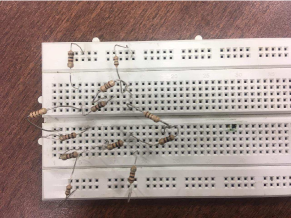
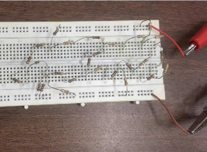
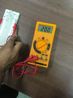
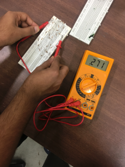
Fig. 12: (a) Setup of $2\times 2$ square network and (b) $2\times 2$ hexagonal network on a breadboard. Multimeter’s reading of $R_{\text{eff}}$ for (c) the square and (d) hexagonal networks. Each resistor in the networks has resistance $R=100$ $\Omega$.

We then connect the networks to a DC power supply (manufactured by Keltronix, India) and determined the effective resistance by measuring the voltage and current across the circuit (figure 13). The following are the readings obtained for the $2\times 2$ square and hexagonal networks.

Table 1: Rectangular/square case

V (Volts)	I (Amperes)
3.01	0.017
3.48	0.019
4.01	0.022
4.49	0.024
5.01	0.027
5.63	0.03
6.01	0.032
6.51	0.035
7.06	0.037
7.47	0.04
7.95	0.042
8.47	0.045
9.16	0.048
9.49	0.05
10.13	0.053
10.53	0.055
11.06	0.058
11.49	0.06
12.3	0.064
13.02	0.068
13.5	0.07
14.06	0.073
14.71	0.076
15.1	0.078

Table 2: Hexagonal (armchair) case

V (Volts)	I (Amperes)
2.54	0.013
3.52	0.015
4	0.017
4.55	0.019
5	0.021
5.52	0.023
6.15	0.025
6.52	0.026
7.08	0.029
7.5	0.03
8.06	0.032
8.48	0.034
9.02	0.036
9.5	0.038
10.06	0.04
10.45	0.041
11.05	0.043
11.59	0.045
12.09	0.047
12.46	0.049
13.02	0.051
13.49	0.053
14.03	0.055
14.74	0.057
15.1	0.059

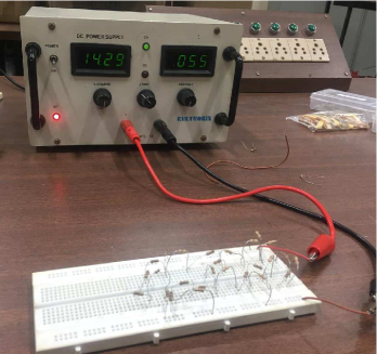
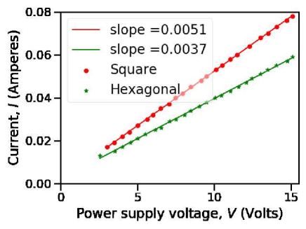
Fig. 13: (a) Setup for determining internal resistance using voltage regulator. The resistance is obtained by dividing the value of voltage by the value of current. (b) Current vs voltage plots for square and hexagonal lattices. The slopes $s$ of the curves estimate the values of $R_{\text{eff}}$ ($R_{\text{eff}}=1/G_{\text{eff}}$). Here we find $R_{\text{eff}}=196.08\,\Omega$ for the square network and $R_{\text{eff}}=270.27\,\Omega$ for the hexagonal network.

From the above two tables, we plot the $I$-$V$ (current vs voltage) curves and fit each of them with linear regression lines using the least square method [25]. The slopes of the regression lines estimate the values of conductance, $G_{\text{eff}}=1/R_{\text{eff}}$. We find $G_{\text{eff}}=0.0051\,\Omega{{}^{-1}}$ and $G_{\text{eff}}=0.0037\,\Omega{{}^{-1}}$, implying $R_{\text{eff}}=196.08\,\Omega$ and $R_{\text{eff}}=270.27\,\Omega$ for case $A$ (square) and $B$ (hexagonal) respectively. The values are slightly off the theoretical values: 1.96% below for case A and 0.43% below for case B. In case A, the root mean square error (RMSE) and coefficient of determination ($R^{2}$ score) [25] of the regression line are 5.76$\times 10^{-8}$ and 0.999831 respectively. The same for case B are 1.6$\times 10^{-7}$ and 0.999139 respectively. The values reflect that regression lines have reasonably high accuracy. The lines, however, show very small finite intercepts of values $0.00158$ and $0.00226$ Amperes. These offset values possibly originate from the resistances in the circuit connection (breadboard and wire connections to the power supply) since we have already checked that the networks accurately produce the theoretical result when measured separately with a multimeter. Thus as inference, we must say that our experiment validates the theory within very low error bars. The Python codes of our experimental plots and regression analysis can be found at https://github.com/hbaromega/2D-Resistor-Network/tree/master/EXPT.

8 Outlook

The detailed but simple derivations of finite size lattice networks of three distinct geometries and the discussed simple experiment on a breadboard setup offer very easy and effective way to teach network analysis to students or even adults since the background requirement is minimal (only Kirchhoff’s laws and a programming language). Therefore, this can be added to one of the earlier proposed curricula [26] in this regard. Later, such studies can be connected to the graph theory since graphs offer visual appeal to one’s learning and conceptual comprehensibility.

Appendix A Linearization of V-matrix

The KCL equations contain two-dimensional $V_{i,j}$ elements. For the rectangular or triangular lattice, when we linearize it to a one-dimensional vector or column matrix, we take either of these two mappings:
Mapping 1:

$$V_{1,1},\cdots,V_{L_{x},1} \to V_{1},\cdots,V_{L_{x}}\,.$$

$$V_{1,2},\cdots,V_{L_{x},2} \to V_{L_{x}+1},\cdots,V_{2L_{x}}\,.$$

$$\vdots$$

$$V_{1,L_{y}},\cdots,V_{L_{x},L_{y}} \to V_{(L_{y}-1)L_{x}+1},\cdots,V_{L_{y}L_{x}}\,.$$

$$\text{Generically,}\quad(i,j) \to(j-1)L_{x}+i\,.$$ (52)

Mapping 2:

$$V_{1,1},\cdots,V_{1,L_{y}} \to V_{1},\cdots,V_{L_{y}}\,.$$

$$V_{2,1},\cdots,V_{2,L_{y}} \to V_{L_{y}+1},\cdots,V_{2L_{y}}\,.$$

$$\vdots$$

$$V_{L_{x},1},\cdots,V_{L_{x},L_{y}} \to V_{(L_{x}-1)L_{y}+1},\cdots,V_{L_{x}L_{y}}\,.$$

$$\text{Generically,}\quad(i,j) \to(i-1)L_{y}+j\,.$$ (53)

Now a typical equation such as Eq. (16) looks like

$$\alpha V_{1}+\beta V_{2}+\cdots+\gamma V_{L_{x}}=I_{1}\,.$$ (54)

which can be recast as

$$G_{11}V_{1}+G_{12}V_{2}+\cdots+G_{1L_{x}}V_{L_{x}}=I_{1}\,.$$ (55)

Generically this can be written as

$$G_{i1}V_{1}+G_{i2}V_{2}+\cdots+G_{iL_{x}}V_{L_{x}}=I_{i}\,.$$ (56)

which builds the matrix form:

$$\begin{bmatrix}G_{11}&G_{12}&\cdots&G_{1N_{L}}\\ G_{21}&G_{22}&\cdots&G_{1N_{L}}\\ \vdots&\vdots&\ddots&\vdots\\ G_{N_{L}1}&G_{N_{L}2}&\cdots&G_{N_{L}N_{L}}\end{bmatrix}\begin{bmatrix}V_{1}\\ V_{2}\\ \vdots\\ V_{N_{L}}\end{bmatrix}=\begin{bmatrix}I_{1}\\ I_{2}\\ \vdots\\ I_{N_{L}}\end{bmatrix}\,.$$ (57)

where $N_{L}\equiv L_{x}L_{y}$.

Finding corresponding row and column of ${\bf G}$, given row of ${\bf I}$:

Since each lattice point follows a particular KCL depending on its neighborhood and voltage connection, the rank of that lattice (reflected by the row or index $i$ of current vector $I$ in Eq. (56)) in the mapped 1D array will denote the row of ${\bf G}$ and the index of ${\bf V}$ (which is a vector or column matrix) will yield the column of ${\bf G}$.

Mapping in the hexagonal lattice case:

Since we introduce another index $k$ in the armchair hexagonal lattice, we extend the linear mapping as

$$(i,j,k)\to i+(j-1)L_{x}+kL_{x}L_{y}\,.$$ (58)

One can check the mapping conserves the total number of points $N_{\text{site}}=L_{x}(2L_{y}+1)$:

$k=0$ case:

$$V_{1,1,0},\cdots,V_{L_{x},1,0} \to V_{1},\cdots,V_{L_{x}}\,.$$

$$V_{1,2,0},\cdots,V_{L_{x},2,0} \to V_{L_{x}+1},\cdots,V_{2L_{x}}\,.$$

$$\vdots$$

$$V_{1,L_{y},0},\cdots,V_{L_{x},L_{y},0} \to V_{(L_{y}-1)L_{x}+1},\cdots,V_{L_{y}L_{x}}\,.$$

$k=1$ case:

$$V_{1,1,1},\cdots,V_{L_{x},1,1} \to V_{L_{x}L_{y}+1},\cdots,V_{(L_{y}+1)L_{x}}\,.$$

$$V_{1,2,1},\cdots,V_{L_{x},2,1} \to V_{(L_{y}+1)L_{x}+1},\cdots,V_{(L_{y}+2)L_{x}}\,.$$

$$\vdots$$

$$V_{1,L_{y},1},\cdots,V_{L_{x},L_{y},1} \to V_{(2L_{y}-1)L_{x}+1},\cdots,V_{2L_{y}L_{x}}\,.$$

$$V_{1,L_{y}+1,1},\cdots,V_{L_{x},L_{y}+1,1} \to V_{(2L_{y}L_{x}+1},\cdots,V_{(2L_{y}+1)L_{x}}\,.$$

References

References

- [1] I.E. Irodov. Problems in General Physics. Mir Publishers, 1981.
- [2] J. Bird. Electrical Circuit Theory and Technology. Newnes, 2010.
- [3] Keji Lai, Masao Nakamura, Worasom Kundhikanjana, Masashi Kawasaki, Yoshinori Tokura, Michael A. Kelly, and Zhi-Xun Shen. Mesoscopic percolating resistance network in a strained manganite thin film. Science, 329(5988):190–193, 2010.
- [4] Zhenhua Wu, Eduardo López, Sergey V. Buldyrev, Lidia A. Braunstein, Shlomo Havlin, and H. Eugene Stanley. Current flow in random resistor networks: The role of percolation in weak and strong disorder. Phys. Rev. E, 71:045101, Apr 2005.
- [5] Scott Kirkpatrick. Percolation and conduction. Rev. Mod. Phys., 45:574–588, Oct 1973.
- [6] J. Bernasconi. Conduction in anisotropic disordered systems: Effective-medium theory. Phys. Rev. B, 9:4575–4579, May 1974.
- [7] J Koplik. On the effective medium theory of random linear networks. Journal of Physics C: Solid State Physics, 14(32):4821–4837, nov 1981.
- [8] Pedro G. Toledo, H.Ted Davis, and L.E. Scriven. Transport properties of anisotropic porous media: effective medium theory. Chemical Engineering Science, 47(2):391 – 405, 1992.
- [9] Kang Wu and R. Mark Bradley. Efficient green’s-function approach to finding the currents in a random resistor network. Phys. Rev. E, 49:1712–1725, Feb 1994.
- [10] József Cserti. Application of the lattice green’s function for calculating the resistance of an infinite network of resistors. American Journal of Physics, 68(10):896–906, 2000.
- [11] M. Q. Owaidat and J. H. Asad. Resistance calculation of pentagonal lattice structure of resistors. Communications in Theoretical Physics, 71(8):935, aug 2019.
- [12] F Y Wu. Theory of resistor networks: the two-point resistance. Journal of Physics A: Mathematical and General, 37(26):6653–6673, jun 2004.
- [13] Zhi zhong Tan, Ling Zhou, and Jian-Hua Yang. The equivalent resistance of a 3 x n cobweb network and its conjecture of a m x ncobweb network. Journal of Physics A: Mathematical and Theoretical, 46(19):195202, apr 2013.
- [14] John W. Essam, Nikolay Sh. Izmailyan, Ralph Kenna, and Zhi-Zhong Tan. Comparison of methods to determine point-to-point resistance in nearly rectangular networks with application to a ‘hammock’ network. Royal Society Open Science, 2(4):140420, 2015.
- [15] Zhi-Zhong Tan and Zhen Tan. The basic principle of m x n resistor networks. Communications in Theoretical Physics, 72(5):055001, apr 2020.
- [16] Zhi-Zhong Tan and Zhen Tan. Electrical properties of an m x n rectangular network. Physica Scripta, 95(3):035226, feb 2020.
- [17] Mikhail Kagan. On equivalent resistance of electrical circuits. Am. J. Phys., 83, 2015.
- [18] F. Dörfler, J. W. Simpson-Porco, and F. Bullo. Electrical networks and algebraic graph theory: Models, properties, and applications. Proceedings of the IEEE, 106(5):977–1005, 2018.
- [19] B. Bollobas. Modern Graph Theory. Graduate Texts in Mathematics. Springer New York, 2013.
- [20] G. Kirchhoff. Ueber die auflösung der gleichungen, auf welche man bei der untersuchung der linearen vertheilung galvanischer ströme geführt wird. Annalen der Physik, 148(12):497–508, 1847.
- [21] G. Kirchhoff. On the solution of the equations obtained from the investigation of the linear distribution of galvanic currents. IRE Transactions on Circuit Theory, 5(1):4–7, 1958.
- [22] J. O’Malley. Schaum’s Outline of Basic Circuit Analysis, Second Edition. Schaum’s Outline Series. McGraw-Hill Education, 2011.
- [23] B Derrida and J Vannimenus. A transfer-matrix approach to random resistor networks. Journal of Physics A: Mathematical and General, 15(10):L557–L564, oct 1982.
- [24] A. H. Castro Neto, F. Guinea, N. M. R. Peres, K. S. Novoselov, and A. K. Geim. The electronic properties of graphene. Rev. Mod. Phys., 81:109–162, Jan 2009.
- [25] D.C. Montgomery, E.A. Peck, and G.G. Vining. Introduction to Linear Regression Analysis. Wiley Series in Probability and Statistics. Wiley, 2015.
- [26] A. Porebska, P. Schmidt, and P. Zegarmistrz. The use of various didactic approaches in teaching of circuit analysis. In 2014 International Conference on Signals and Electronic Systems (ICSES), pages 1–4, 2014.