Compositional equivalences based on Open pNets

Abstract.

Establishing equivalences between programs or systems is crucial both for verifying correctness of programs, by establishing that two implementations are equivalent, and for justifying optimisations and program transformations, by establishing that a modified program is equivalent to the source one. There exist several equivalence relations for programs, and bisimulations are among the most versatile of these equivalences. Among bisimulation relations one distinguishes strong bisimulation, that requires that each action of a program is simulated by a single action of the equivalent program, a weak bisimulation that is a coarser relation, allowing some of the actions to be invisible or internal moves, and thus not simulated by the equivalent program.

pNet is a generalisation of automata that model open systems. They feature variables and hierarchical composition. Open pNets are pNets with holes, i.e. placeholders inside the hierarchical structure that can be filled later by sub-systems.

This article defines bisimulation relations for the comparison of systems specified as pNets. We first define a strong bisimulation for open pNets. We then define an equivalence relation similar to the classical weak bisimulation, and study its properties. Among these properties we are interested in compositionality: if two systems are proven equivalent they will be undistinguishable by their context, and they will also be undistinguishable when their holes are filled with equivalent systems. We identify sufficient conditions on the automata to ensure compositionality of strong and weak bisimulation. The article is illustrated with a transport protocol running example; it shows the characteristics of our formalism and our bisimulation relations.

1. Introduction

In the nineties, several works extended the basic behavioural models based on labelled transition systems to address value-passing or parameterised systems, using various symbolic encodings of the transitions [De 85, Lar87]. These works use the term parameter to designate systems where variables that have a strong influence the system structure and behaviour. In parameterised systems, parameters can typically be the number of processes in the system or the way they interact. In [IL01, HL95], Lin, Ingolfsdottir and Hennessy developed a full hierarchy of bisimulation equivalences, together with a proof system, for value passing CCS, including notions of symbolic behavioural semantics and various symbolic bisimulations (early and late, strong and weak, and their congruent versions). They also extended this work to models with explicit assignments [Lin96]. Separately J. Rathke [HR98] defined another symbolic semantics for a parameterised broadcast calculus, together with strong and weak bisimulation equivalences, and developed a symbolic model-checker based on a tableau method for these processes. 30 years later, no practical verification approach and no verification platform are using this kind of approaches to provide proof methods for value-passing processes or open process expressions.

This article provides a theoretical background that allows us to implement such a verification platform. We build upon the concept of pNets that allowed us to give a behavioural semantics of distributed components and verify the correctness of distributed applications in the past 15 years. pNets is a low level semantic framework for expressing the behaviour of various classes of distributed languages, and as a common internal format for our tools. pNets allow the specification of parameterised hierarchical labelled transition systems: labelled transition systems with parameters can be combined hierarchically.

We develop here a semantics for a model of interacting processes with parameters and holes. Our approach is originally inspired from Structured Operational Semantics with conditional premisses as in [Gro93, van04]. But we aim at a more constructive and implementable approach to compute the semantics (intuitively transitions including first order predicates) and to check equivalences for these open systems. The main interest of our symbolic approach is to define a method to prove properties directly on open structures; these properties will then be preserved by any correct instantiation of the holes. As a consequence, our model allows us to reason on composition operators as well as on full-size distributed systems. The parametric nature of the model and the properties of compositionability of the equivalence relations are thus the main strengths of our approach.

pNets and open automata

pNet is a convenient model to model concurrent systems in a hierarchical and parameterised way. The coordination between processes is expressed as synchronisation vectors that allow the definition of complex and expressive synchronisation patterns. Open pNets are pNets for which some elements in the hierarchy are still undefined, such undefined elements are called holes; a hole can be filled later by providing another pNet. The semantics of pNets can be expressed as a translation to a labelled transition system, but only if the pNet has no parameter and no hole. Adding parameters to a LTS is quite standard but enabling holes inside LTSs is not a well-defined notion. We thus define open automata that can be seen as LTSs with parameters and holes. The transitions of open automata are much more complex than transitions of an LTS as the firing on a transition depends on parameters and actions that are symbolic. This article defines the notion of open transition a transition that is symbolic in terms of parameters and coordinated actions.

Contrarily to pNets, open automata are not hierarchical structures, thus they are more convenient for formal reasoning but not adapted to the definition of a complex and structured system like pNets. Additionally, open transitions are expressed in terms of logics more than in terms of synchronised actions, synchronisation vectors on the contrary make it easy to express synchronisations that exist in process algebra or in specification and high-level languages for distributed systems.

This article defines pNets and illustrates with an example how they can be used to provide the model of a communicating system. Then we introduce open automata to provide a semantics to open pNets and introduce bisimulation relations and their properties. Open automata can be also seen as an algebra that can be studied independently from its application to pNets but their composition properties make more sense in a hierarchical model like pNets.

Previous Works and Contribution

While most of our previous works relied on closed, fully-instantiated semantics [BABC⁺09, ABHK⁺17, HKM16], it is only recently that we could design a first version of a parameterised semantics for pNets with a strong bisimulation equivalence [HMZ16]. This article builds upon this previous parameterised semantics and provides a clean and complete version of the semantics with a slightly simplified formalism that makes proofs easier. It also adds a notion of global state to automata. Also, in [HMZ16] the study of compositionability was only partial, and in particular the proof that bisimulation is an equivalence is one new contribution of this article and provides a particularly interesting insight on the semantic model we use. The new formalism allowed us to extend the work and define weak bisimulation for open automata, which is entirely new. This allows us to define a weak bisimulation equivalence for open pNets with valuable properties of compositionality. To summarise, the contribution of this paper are the following:

• The definition of open automata: an algebra of parameterised automata with holes, and a strong bisimulation equivalence. This is an adaptation of [HMZ16] with an additional property stating that strong bisimulation equivalence is indeed an equivalence relation.

• A semantics for open pNets expressed as translation to open automata. This is an adaptation of [HMZ16] with a complete proof that strong bisimulation is compositional.

• A theory of weak bisimulation for open automata, and its properties. It relies on the definition of weak open transitions that are derived from transitions of the open automaton by concatenating invisible action transitions with one (visible or not) action transition. The precise and sound definition of the concatenation is also a major contribution of this article.

• A resulting weak bisimulation equivalence for open pNets and a simple static condition on synchronisation vectors inside pNets that is sufficient to ensure that weak bisimulation is compositional.

• An illustrative example based on a simple transport protocol, showing the construction of the weak open transitions, and the proof of weak bisimulation.

What is new about open automata bisimulation?

Bisimulation over a symbolic and open model like open pNets or open automata is different from the classical notion of bisimulation because it cannot rely on the equality over a finite set of action labels. Classical bisimulations require to exhibit, for each transition of one system, a transition of the other system that simulates it. Instead, bisimulation for open automata relies on the simulation of each open transition of one automaton by a set of open transitions of the other one, that should cover all the cases where the original transition can be triggered.

Compositionality of bisimulation in our model come from the specification of the interactions, including actions of the holes. In pNets, synchronisation vectors define the possible interactions between the pNet that fills the hole and the surrounding pNets. In open automata, this is reflected by symbolic hypotheses that depend on the actions of the holes. This additional specification is the price to pay to obtain the compositionality of bisimulation that cannot be guaranteed in traditional process algebras.

This approach also allows us to specify a sufficient condition on allowed transitions to make weak bisimulation compositional; namely it is not possible to synchronise on invisible actions from the holes or prevent them to occur.

Structure

This article is organised as follows. Section 2 provides the definition of pNets and introduces the notations used in this paper, including the definition of open pNets. Section 3 defines open automata, i.e. automata with parameters and transitions conditioned by the behaviour of “holes”; a strong bisimulation equivalence for open automata is also presented in this section. Section 4 gives the semantics of open pNets expressed as open automata, and states compositional properties on the strong bisimulation for open pNets. Section 5 defines a weak bisimulation equivalence on open automata and derives weak bisimilarity for pNets, together with properties on compositionality of weak bisimulation for open pNets. Finally, Section 6 discusses related works and Section 7 concludes the paper.

2. Background and notations

This section introduces the notations we will use in this article, and recalls the definition of pNets [HMZ16] with an informal semantics of the pNet constructs. The only significant difference compared to our previous definitions is that we remove here the restriction that was stating that variables should be local to a state of a labelled transition system.

2.1. Notations

Term algebra.

Our models rely on a notion of parameterised actions, that are symbolic expressions using data types and variables. As our model aims at encoding the low-level behaviour of possibly very different programming languages, we do not want to impose one specific algebra for denoting actions, nor any specific communication mechanism. So we leave unspecified the constructors of the algebra that will allow building expressions and actions. Moreover, we use a generic action interaction mechanism, based on (some sort of) unification between two or more action expressions, to express various kinds of communication or synchronisation mechanisms.

Formally, we assume the existence of a term algebra $\mathbb{T}$, and denote as $\Sigma$ the signature of the data and action constructors. Within $\mathbb{T}$, we distinguish a set of data expressions $\mathbb{E}$, including a set of boolean expressions $\mathbb{E}$ ($\mathbb{B}\subseteq\mathbb{E}$), and a set of action expressions $\mathbb{E}$ called the action algebra $\mathbb{A}$, with $\mathbb{A}\subseteq\mathbb{T},\mathbb{E}\cap\mathbb{A}=\emptyset$; naturally action terms will use data expressions as sub-terms. The function $\makebox{\it vars}(t)$ identifies the set of variables in a term $t\in\mathbb{T}$.

We let $e_{i}$ range over expressions ($e_{i}\in\mathbb{E}$), $a$ range over action labels, op be operators, and $x_{i}$ and $y_{i}$ range over variable names.

We define two kinds of parameterised actions. The first kind distinguishes input variables and the second kind does not. We first define the set of actions that distinguish input variables, they will be used in the definition of pLTS below:

$$\begin{array}[l]{rcl@{\quad}p{7.5cm}}\alpha\in\mathbb{A}&::=&a(p_{1},\ldots,p_{n})&\text{action terms}\\ p_{i}&::=&?x~{}|~{}e_{i}&\text{parameters (input variable or expression)}\\ e_{i}&::=&\makebox{\it Value}~{}|~{}x~{}|~{}\makebox{\it op}(\makebox{\it e}_{1},..,\makebox{\it e}_{n})&\text{Expressions}\end{array}$$

The input variables in an action term are those marked with a ?. We additionally impose that each input variable does not appear somewhere else in the same action term: $p_{i}=?x\Rightarrow\forall j\neq i.\,x\notin\makebox{\it vars}(p_{j})$. We define $iv(t)$ as the set of input variables of a term $t$ (without the ’?’ marker). Action algebras can encode naturally usual point-to-point message passing calculi (using $a(?x_{1},...,?x_{n})$ for inputs, $a(v_{1},..,v_{n})$ for outputs), but it also allows for more general synchronisation mechanisms, like gate negotiation in Lotos, or broadcast communications.

The set of actions that do not distinguish input variables is denoted $\mathbb{A}_{S}$, it will be used in synchronisation vectors of pNets:

$$\begin{array}[l]{rcl@{\quad}l}\alpha\in\mathbb{A}_{S}&::=&a(e_{1},\ldots,e_{n})\end{array}$$

Indexed sets

In this article, we extensively use indexed structures (maps) over some countable indexed sets. The indices can typically be integers, bounded or not. We use indexed sets in pNets because we want to consider a set of processes, and specify separately how to synchronise them. Roughly this could also be realised using tuples, however indexed sets are more general, can be infinite, and give a compact representation than using the position in a possibly long tuple.

An indexed family is denoted as follows: $t_{i}^{i\in I}$ is a family of elements $t_{i}$ indexed over the set $I$. Such a family is equivalent to the mapping $(i\text{\scriptsize{$\mapsto$}}t_{i})^{i\in I}$, and we will also use mapping notations to manipulate indexed sets. To specify the set over which the structure is indexed, indexed structures are always denoted with an exponent of the form $i\in I$.

Consequently, $t_{i}^{i\in I}$ defines first $I$ the set over which the family is indexed, and then $t_{i}$ the elements of the family. For example $t_{i}^{i\in\{3\}}$ is the mapping with a single entry $t_{3}$ at index $3$; exceptionally, for mappings with only a few entries we use the notation $(3\text{\scriptsize{$\mapsto$}}t_{3})$ instead. In this article, sentences of the form “there exists $t_{i}^{i\in I}$” means there exists $I$ and a function that maps each element of $I$ to a term $t_{i}$.

When this is not ambiguous, we shall use abusive notations for sets, and typically write “indexed set over I” when formally we should speak of multisets, and “$x\in A_{i}^{i\in I}$” to mean $\exists i\in I.\,x=A_{i}$. To simplify equations, an indexed set can be denoted $\overline{t}$ instead of $t_{i}^{i\in I}$ when $I$ is irrelevant.

The disjoint union on sets is $\uplus$. We extend it to disjoint union of indexed sets defined by the merge of the two sets provided they are indexed on disjoint families. The elements of the union of two indexed sets are then accessed by using an index of one of the two joined families. The standard subtraction operation on indexed sets is $\setminus$, with $\operatorname{dom}(A\setminus B)=\operatorname{dom}(A)\setminus B$.

Substitutions

This article also uses substitutions. Applying a substitution inside a term $t$ is denoted $t\{\{\!y_{i}\leftarrow e_{i}\}\}^{i\in I}$ and consists in replacing in parallel all the occurrences of variables $y_{i}$ in the term $t$ by the terms $e_{i}$. Note that a substitution is defined by a partial function that is applied on the variables inside a term. We let Post range over partial functions that are used as substitution and use the notation $\{y_{i}\leftarrow e_{i}\}^{i\in I}$ to define such a partial function. These partial functions are sometimes called substitution functions in the following. Thus, $\{\{\!\makebox{\it Post}\}\}$ is the operation that applies, in a parallel manner, the substitution defined by the partial function Post. $\odot$ is a composition operator on these partial functions, such that for any term $t$ we have: $t\{\{\!\makebox{\it Post}\!\odot\!\makebox{\it Post}^{\prime}\}\}=(t\{\{\!\makebox{\it Post}^{\prime}\}\})\{\{\!\makebox{\it Post}\}\}$. This property must also be valid when the substitution does not operate on all variables. We thus define a composition operation as follows:

$$(x_{k}\leftarrow e_{k})^{k\in K}\!\odot\!(x^{\prime}_{k^{\prime}}\leftarrow e^{\prime}_{k^{\prime}})^{k^{\prime}\in K^{\prime}}=(x_{k}\leftarrow e_{k}\{\{\!(x^{\prime}_{k^{\prime}}\leftarrow e^{\prime}_{k^{\prime}})^{k^{\prime}\in K^{\prime}}\}\})^{k\in K}\cup(x^{\prime}_{k^{\prime}}\leftarrow e^{\prime}_{k^{\prime}})^{k^{\prime}\in K^{\prime\prime}}$$

where $K^{\prime\prime}=\{k^{\prime}\in K^{\prime}|x^{\prime}_{k^{\prime}}\not\in\{x_{k}\}^{k\in K}\}$

2.2. Parameterised Networks (pNets)

pNets are tree-like structures, where the leaves are either parameterised labelled transition systems (pLTSs), expressing the behaviour of basic processes, or holes, used as placeholders for unknown processes. Nodes of the tree (pNet nodes) are synchronising artefacts, using a set of synchronisation vectors that express the possible synchronisation between the parameterised actions of a subset of the sub-trees.

A pLTS is a labelled transition system with variables; variables can be used inside states, actions, guards, and assignments. Note that we make no assumption on finiteness of the set of states nor on finite branching of the transition relation. Compared to our previous works [HMZ16, ABHK⁺17] we extend the expressiveness of the model by making variables global.

[pLTS] A pLTS is a tuple $\makebox{\it pLTS}\triangleq\langle\langle S,s_{0},V,\to\rangle\rangle$ where:

• $S$ is a set of states.

• $s_{0}\in S$ is the initial state.

• $V$ is a set of global variables for the pLTS.

• $\to\subseteq S\times L\times S$ is the transition relation and $L$ is the set of labels of the form:
  $\langle\alpha,~{}e_{b},~{}(x_{j}\!:={e}_{j})^{j\in J}\rangle$, where $\alpha\in\mathbb{A}$ is a parameterised action, $e_{b}\in\mathbb{B}$ is a guard, and the variables $x_{j}$ are assigned the expressions $e_{j}\in\mathbb{E}$. If $s\xrightarrow{\langle\alpha,~{}e_{b},~{}(x_{j}\!:={e}_{j})^{j\in J}\rangle}s^{\prime}\in\to$ then $\makebox{\it vars}(\alpha)\backslash\makebox{\it iv}(\alpha)\!\subseteq\!V$, $\makebox{\it vars}(e_{b})\!\subseteq\!\makebox{\it vars}(s)\cup\makebox{\it vars}(\alpha)$, and $\forall j\!\in\!J.\,\left(\makebox{\it vars}(e_{j})\!\subseteq\!V\cup\makebox{\it iv}(\alpha)\land x_{j}\!\in V\right)$.

The semantics of the assignments is that a set of assignments between two states is performed in parallel so that their order do not matter and they all use the values of variables before the transition (or the values received as action parameters).

Now we define pNet nodes as constructors for hierarchical behavioural structures. A pNet has a set of sub-pNets that can be either pNets or pLTSs, and a set of holes, playing the role of process parameters. A pNet is thus a composition operator that can receive processes as parameters; it expresses how the actions of the sub-processes synchronise.

Each sub-pNet exposes a set of actions, called internal actions. The synchronisation between global actions exposed by the pNet and internal actions of its sub-pNets is given by synchronisation vectors: a synchronisation vector synchronises one or several internal actions, and exposes a single resulting global action.

We now define the structure of pNets, the following definition relies on the definition of holes, leaves and sorts formalised below in Definition 2.2. Informally, holes are process parameters, leaves provide the set of pLTSs at the leaves of the hierarchical structure of a pNet, and sorts give the signature of a pNet, i.e. the actions it exposes.

[pNets] A pNet $P$ is a hierarchical structure where leaves are pLTSs and holes
$P\triangleq\makebox{\it pLTS}~{}|~{}\langle\langle P_{i}^{i\in I},\makebox{\it Sort}_{j}^{j\in J},\makebox{\it SV}_{k}^{k\in K}\rangle\rangle$ where:

• $I$ is a set of indices and $P_{i}^{i\in I}$ is the family of sub-pNets indexed over $I$. $vars(P_{i})$ and $vars(P_{j})$ must be disjoint for $i\neq j$.

• $J$ is a set of indices, called holes. $I$ and $J$ are disjoint: $I\!\cap\!J=\emptyset$, $I\!\cup\!J\neq\emptyset$.

• $\makebox{\it Sort}_{j}\subseteq\mathbb{A}_{S}$ is a set of action terms, denoting the sort of hole $j$.

• $\makebox{\it SV}_{k}^{k\in K}$ is a set of synchronisation vectors. $\forall k\!\in\!K.\,\makebox{\it SV}_{k}\!=\!\alpha_{l}^{l\in I_{k}\uplus J_{k}}\to\alpha^{\prime}_{k}[e_{k}]$ where $\alpha^{\prime}_{k}\in\mathbb{A}_{S}$, $I_{k}\subseteq I$, $J_{k}\subseteq J$, $\forall i\!\in\!I_{k}.\,\alpha_{i}\!\in\!\makebox{\it Sort}(P_{i})$, $\forall j\!\in\!J_{k}.\,\alpha_{j}\!\in\!\makebox{\it Sort}_{j}$, and $\makebox{\it vars}(\alpha^{\prime}_{k})\subseteq\bigcup_{l\in I_{k}\uplus J_{k}}{\makebox{\it vars}({\alpha_{l}})}$. The global action of a vector $\makebox{\it SV}_{k}$ is $\alpha^{\prime}_{k}$. $e_{k}\in\mathbb{B}$ is a guard associated to the vector such that $\makebox{\it vars}(e_{k})\subseteq\bigcup_{l\in I_{k}\uplus J_{k}}{\makebox{\it vars}({\alpha_{l}})}$.

Synchronisation vectors are identified modulo renaming of variables that appear in their action terms.

The preceding definition relies on the auxiliary functions defined below:

[Sorts, Holes, Leaves, Variables of pNets]

• The sort of a pNet is its signature, i.e. the set of actions in $\mathbb{A}_{S}$ it can perform, where each action signature is an action label plus the arity of the action.

  $$\begin{array}[]{l}\operatorname{Sort}(\langle\langle S,s_{0},V,\to\rangle\rangle)=\{\operatorname{Sort}(\alpha)|s\xrightarrow{\langle\alpha,~{}e_{b},~{}(x_{j}\!:={e}_{j})^{j\in J}\rangle}s^{\prime}\in\to\}\\ \operatorname{Sort}(\langle\langle\overline{P}\!,\overline{\makebox{\it Sort}},\overline{\makebox{\it SV}\,}\rangle\rangle)=\{\operatorname{Sort}(\alpha^{\prime})|\,\overline{\alpha}\to\alpha^{\prime}[e_{b}]\in\overline{\makebox{\it SV}}\,\}\\ \operatorname{Sort}(\alpha(p_{1},..,p_{n}))=(\alpha,n)\end{array}$$

• The set of variables of a pNet $P$, denoted $vars(P)$ is disjoint union the set of variables of all pLTSs that compose $P$.

• The set of holes $\operatorname{Holes}(P)$ of a pNet is the indices of the holes of the pNet itself plus the indices of all the holes of its sub-pNets. It is defined inductively (we suppose those indices disjoints):

  $$\begin{array}[]{l}\operatorname{Holes}(\langle\langle S,s_{0},V,\to\rangle\rangle)\!=\!\emptyset\\ \operatorname{Holes}(\langle\langle P_{i}^{i\in I}\!,\overline{\makebox{\it Sort}},\overline{\makebox{\it SV}}\rangle\rangle)=J\uplus{\displaystyle\bigcup_{i\in I}\operatorname{Holes}(P_{i})}\\ \forall i\in I.\,\operatorname{Holes}(P_{i})\cap J=\emptyset\\ \forall i_{1},i_{2}\in I.\,i_{1}\neq i_{2}\Rightarrow\operatorname{Holes}(P_{i_{1}})\cap\operatorname{Holes}(P_{i_{2}})=\emptyset\end{array}$$

• The set of leaves of a pNet is the set of all pLTSs occurring in the structure, as an indexed family of the form $\operatorname{Leaves}(P)=\langle\langle P_{i}\rangle\rangle^{i\in L}$.

  $$\begin{array}[]{l}\operatorname{Leaves}(\langle\langle S,s_{0},V,\to\rangle\rangle)\!=\!\emptyset\\ \operatorname{Leaves}(\langle\langle P_{i}^{i\in I}\!,\overline{\makebox{\it Sort}}\!,\overline{\makebox{\it SV}\,}\rangle\rangle)={\displaystyle\biguplus_{i\in I}\operatorname{Leaves}(P_{i})\uplus\{i\text{\scriptsize{$\mapsto$}}P_{i}|P_{i}\text{ is a }\makebox{\it pLTS}\}}\end{array}$$

A pNet $Q$ is closed if it has no hole: $\operatorname{Holes}(Q)=\emptyset$; else it is said to be open. Sort comes naturally with a compatibility relation that is similar to a type-compatibility check. We simply say that two sorts are compatible if they consist of the same actions with the same arity. In practice, it is sufficient to check the equality of the two sets of action signatures of the two sorts.

The informal semantics of pNets is as follows. pLTSs behave more or less like classical automata with conditional branching and variables. The actions on the pLTSs can send or receive values, potentially modifying the value of variables. pNets are synchronisation entities: a pNet node composes several sub-pNets and define how the sub-pNets interact, where a sub-pNet is either a pNet or a pLTS. The synchronisation between sub-pNets is defined by synchronisation vectors (originally introduced by [Arn82]) that express how an action of a sub-pNet can be synchronised with actions of other sub-pNet, and how the resulting synchronised action is visible from outside of the pNet. The synchronisation mechanism is very expressive, including pattern-matching/unification between the parameterized actions within the vector, and an additional predicate over their variables. Consider a pNet node that assembles several pLTSs, the synchronisation vectors specify the way that transitions of the composed pNet are built from the transitions of the sub-nets. This can be seen as "conditional transitions" of the pNet, or alternatively, as a syntax to encode structural operational semantics (SOS rules) of the system: each vector expresses not only the actions emitted by the pNet but also what transitions of the composed pLTSs must occur to trigger this global transition. Synchronisation vectors can also express the exportation of an action of a sub-pNet to the next level, or to hide an interaction and make it non-observable. Finally, a pNet can leave sub-pNets undefined and instead declare holes with a well-defined signature. Holes can then be filled with a sub-pNet. This is defined as follows.

[pNet composition] An open pNet: $P=\langle\langle P_{i}^{i\in I},\makebox{\it Sort}_{j}^{j\in J},\overline{\makebox{\it SV}}\,\rangle\rangle$ can be (partially) filled by providing a pNet $Q$ to fill one of its holes. Suppose $j_{0}\in J$ and $\operatorname{Sort}(Q)\subseteq\makebox{\it Sort}_{j_{0}}$, then:

$$P\left[Q\right]_{j_{0}}=\langle\langle P_{i}^{i\in I}\uplus\{j_{0}\text{\scriptsize{$\mapsto$}}Q\},\makebox{\it Sort}_{j}^{j\in J\setminus\{j_{0}\}},\overline{\makebox{\it SV}}\,\rangle\rangle$$

pNets are composition entities equipped with a rich synchronisation mechanism: synchronisation vectors allow the expression of synchronisation between any number of entities and at the same time the passing of data between processes. Their strongest feature is that the data emitted by processes can be used inside the synchronisation vector to do addressing: it is easy to synchronise a process indexed by $n$ with the action $a(v,n)$ of another process. This is very convenient to model systems and encode futures or message routing.

pNets have been used to model GCM distributed component systems, illustrating the expressiveness of the model [ABHK⁺17]. These works show that pNets are convenient to express the behaviour of the system in a compositional way, which is crucial for the definition of the semantics, especially when dealing with a hierarchical component system. Unfortunately, the semantics of pNets and the existing tools at this point were only able to deal with a closed system completely instantiated: pNets could be used as composition operator in the definition of the semantics, which was sufficient to perform finite-state model checking on a closed system, but there was no theory for the use of pNets as operators and no tool for proving properties on open system. Consequently, much of the formalisation efforts did not use holes and the interplay between holes, sorts, and synchronisation vector was not formalised. In previous works [ABHK⁺17], only closed pNets were equipped with a semantics, it was defined as labelled transition systems which are instantiations of pNets. The theory of pNets as operators able to fully take into account open systems is given in the following sections. Comparing formally the existing direct operational semantics and the semantics derived from open automata in the current article would be an interesting partial proof of soundness for our semantics. The proof could only be partial as the formal semantics that exists only consider closed and fully instantiated pNets. Proving an equivalence between the semantics presented in this article and the operational one shown in [ABHK⁺17] is outside the scope of this article.

2.3. Running Example

To illustrate this work, we use a simple communication protocol, that provides safe transport of data between two processes, over unsafe media.

Figure 1 (left) shows the example principle, which corresponds to the hierarchical structure of a pNet: two unspecified processes $P$ and $Q$ (holes) communicate messages, with a data value argument, through the two protocol entities. Process $P$ sends an p-send(m) message to the Sender; this communication is denoted as in(m). At the other end, process $Q$ receives the message from the Receiver. The holes $P$ and $Q$ can also have other interactions with their environment, represented here by actions p-a and q-b. The underlying network is modelled by a medium entity transporting messages from the sender to the receiver, and that is able to detect transport errors and signal them to the sender. The return ack message from Receiver to Sender is supposed to be safe. The final transmission of the message to the recipient (the hole $Q$) includes the value of the “error counter” $ec$.

Figure 1 (right) shows a graphical view of the pNet SimpleProtocolSpec that specifies the system. The pNet is made of the composition of two pNets: a SimpleSystem node, and a PerfectBuffer sub-pNet. The full system implementation should be equivalent (e.g. weakly bisimilar) to this SimpleProtocolSpec. The pNet has a tree-like structure. The root node of the tree SimpleSystem is the top level of the pNet structure. It acts as the parallel operator. It consists of three nodes: two holes $P$ and $Q$ and one sub-pNet, denoted PerfectBuffer. Nodes of the tree are synchronised using four synchronisation vectors, that express the possible synchronisations between the parameterised actions of a subset of the nodes. For instance, in the vector $<\texttt{p-send(m)},\texttt{in(m)},\_>\rightarrow\texttt{in(m)}$ only $P$ and PerfectBuffer nodes are involved in the synchronisation. The synchronisation between these processes occurs when process $P$ performs p-send(m) action sending a message, and the PerfectBuffer accepts the message through an in(m) action at the same time; the result that will be returned at upper level is the action in(m).

Figure 2 shows the pNet model of the protocol implementation, called SimpleProtocolImpl. When the Medium detects an error (modelled by a local $\tau$ action), it sends back a m-error message to the Sender. The Sender increments its local error counter $ec$, and resends the message (including $ec$) to the Medium, that will, eventually, transmit $m,ec$ to the Receiver.

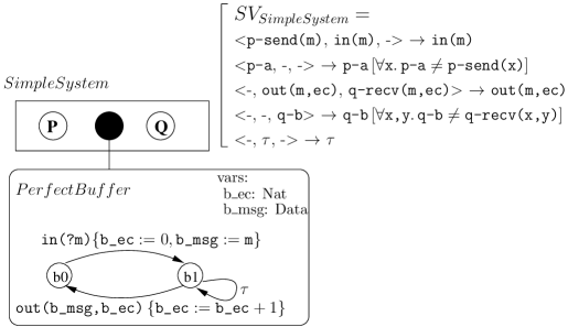
Figure 1. pNet structure of the example and its specification expressed as a pNet called SimpleProtocolSpec

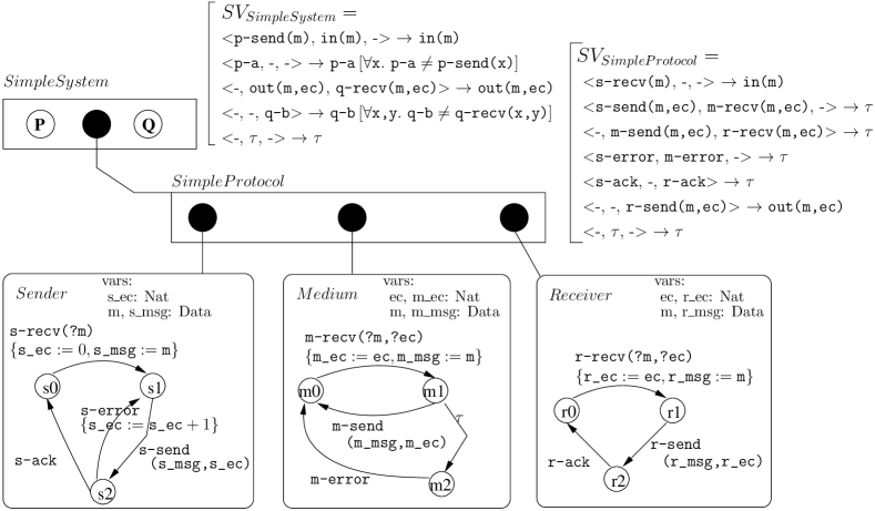
Figure 2. The SimpleProtocolImpl pNet resulting from the composition of the SimpleSystem and the SimpleProtocol pNets.

3. A model of process composition

The semantics of open pNets will be defined as an open automaton. An open automaton is an automaton where each transition composes transitions of several LTSs with action of some holes, the transition occurs if some predicates hold, and can involve a set of state modifications. This section defines open automata and a bisimulation theory for them. This section is an improved version of the formalism described in [HMZ16], extending the automata with a notion of global variable, which makes the state of the automaton more explicit. We also adopt a semantics and logical interpretation of the automata that intuitively can be stated as follows: “if a transition belongs to an open automaton, any refinement of this transition also belongs to the automaton”.

3.1. Open Automata

Open automata (OA) are not composition structures but they are made of transitions that are dependent of the actions of the holes, and they can reason on a set of variables (potentially with only symbolic values). [Open transitions] An open transition (OT) over a set $J$ of holes with sorts $\makebox{\it Sort}_{j}^{j\in J}$, a set $V$ of variables, and a set of states $\mathcal{S}$ is a structure of the form:

$$\cdot \genfrac{}{}{0.0pt}{0}{\hbox{\hskip 26.96095pt\vbox{\hbox{\hskip-26.96095pt\hbox{\hbox{$\displaystyle\displaystyle\beta_{j}^{j\in J^{\prime}},\makebox{\it Pred},\makebox{\it Post}$}}}\vbox{}}}}{\hbox{\hskip 12.82265pt\vbox{\vbox{}\hbox{\hskip-12.82263pt\hbox{\hbox{$\displaystyle\displaystyle s{\color[rgb]{1,0,0}\,\xrightarrow{{\color[rgb]{0,0,0}\alpha}}\,}s^{\prime}$}}}}}}$$

Where $J^{\prime}\subseteq J$ is the set of holes involved in the transition; $s,s^{\prime}\in\mathcal{S}$ are states of the automaton; and $\beta_{j}$ is a transition of the hole $j$, with $\operatorname{Sort}(\beta_{j})\in\makebox{\it Sort}_{j}$. $\alpha$ is the resulting action of this open transition. Pred is a predicate, Post is a set of assignments that are effective after the open transition, they are represented as a substitution function: $({x_{k}\leftarrow e_{k}})^{k\in K}$. Predicates and expressions of an open transition can refer to the variables in $V$, and in the different terms $\beta_{j}$ and $\alpha$. More precisely:

$$\makebox{\it vars}(\makebox{\it Pred})\subseteq V\cup\makebox{\it vars}(\alpha)\cup{\displaystyle\bigcup_{j\in J^{\prime}}\!\!\makebox{\it vars}(\beta_{j})}\quad\land\\ \forall k.\,x_{k}\in V\quad\land\quad\forall k.\,\makebox{\it vars}(e_{k})\subseteq V\cup\makebox{\it vars}(\alpha)\cup{\displaystyle\bigcup_{j\in J^{\prime}}\!\!\makebox{\it vars}(\beta_{j})}$$

The assignments are applied simultaneously because the variables in $V$ can be in both sides ($x_{k}$s are distinct).

Open transitions are identified modulo logical equivalence on their predicate.

It is important to understand the difference between the red dotted rule and a classical inference rule. They correspond to two different logical levels. On one side, classical (black) inference rules use an expressive logic (like any other computer science article). On the other side, open transition rules (with dotted lines) are logical implications, but using a logic with a specific syntax and that can be mechanized (this logic includes the boolean expressions $\mathbb{B}$, boolean operators, and term equality).

An open automaton is an automaton where each transition is an open transition. [Open automaton] An open automaton is a structure
$A=\langle\langle J,\mathcal{S},s_{0},V,\mathcal{T}\rangle\rangle$ where:

• $J$ is a set of indices.

• $\mathcal{S}$ is a set of states and $s_{0}$ an initial state among $\mathcal{S}$.

• $V$ is a set of variables of the automaton and each $v\in V$ may have an initial value $init(v)$.

• $\mathcal{T}$ is a set of open transitions and for each $t\in\mathcal{T}$ there exists $J^{\prime}$ with $J^{\prime}\subseteq J$, such that $t$ is an open transition over $J^{\prime}$ and $\mathcal{S}$.

While the definition and usage of the open transition can be formalised and taken in a pure syntactic acceptance, we take in this article a semantics and logical understanding of open automata. Formally, the open transition sets in open automata are closed by a simple form of refinement that allows us to refine the predicate, or substitute any free variable by an expression as expressed below.

For all predicate Pred for all partial function Post,if $V\!\cap\!\operatorname{dom}(\makebox{\it Post})=\emptyset$, we have:

$${\hbox{{\ooalign{\vphantom{$\displaystyle\genfrac{}{}{0.0pt}{0}{\hbox{\hskip 28.52612pt\vbox{\hbox{\hskip-28.52611pt\hbox{\hbox{$\displaystyle\displaystyle\overline{\beta},\makebox{\it Pred}\,^{\prime},\makebox{\it Post}\,^{\prime}$}}}\vbox{}}}}{\hbox{\hskip 11.74626pt\vbox{\vbox{}\hbox{\hskip-11.74625pt\hbox{\hbox{$\displaystyle\displaystyle t{\color[rgb]{1,0,0}\,\xrightarrow{{\color[rgb]{0,0,0}\alpha}}\,}t^{\prime}$}}}}}}$}\cr{\color[rgb]{1,0,0}\leavevmode\cleaders\hbox to2.20001pt{\raisebox{0.75pt}{\hss$\displaystyle\cdot$\hss}}\hfill\kern 0.0pt}\cr$\displaystyle\genfrac{}{}{0.0pt}{0}{\hbox{\hskip 28.52612pt\vbox{\hbox{\hskip-28.52611pt\hbox{\hbox{$\displaystyle\displaystyle\overline{\beta},\makebox{\it Pred}\,^{\prime},\makebox{\it Post}\,^{\prime}$}}}\vbox{}}}}{\hbox{\hskip 11.74626pt\vbox{\vbox{}\hbox{\hskip-11.74625pt\hbox{\hbox{$\displaystyle\displaystyle t{\color[rgb]{1,0,0}\,\xrightarrow{{\color[rgb]{0,0,0}\alpha}}\,}t^{\prime}$}}}}}}$\cr}}}}\in\mathcal{T}\quad\implies\quad{\hbox{{\ooalign{\vphantom{$\displaystyle\genfrac{}{}{0.0pt}{0}{\hbox{\hskip 94.04019pt\vbox{\hbox{\hskip-94.04018pt\hbox{\hbox{$\displaystyle\displaystyle\overline{\beta}\{\{\!\makebox{\it Post}\}\},\makebox{\it Pred}\,^{\prime}\{\{\!\makebox{\it Post}\}\}\land\makebox{\it Pred},\makebox{\it Post}\!\odot\!\makebox{\it Post}\,^{\prime}$}}}\vbox{}}}}{\hbox{\hskip 106.74199pt\vbox{\vbox{}\hbox{\hskip-106.74199pt\hbox{\hbox{$\displaystyle\displaystyle\mathchoice{\raisebox{-2.0pt}{$\displaystyle\displaystyle t{\color[rgb]{1,0,0}\,\xrightarrow{{\color[rgb]{0,0,0}\alpha\{\{\!\makebox{\it Post}\}\}}}\,}{t^{\prime}}$}}{\raisebox{-2.0pt}{$\displaystyle\textstyle t{\color[rgb]{1,0,0}\,\xrightarrow{{\color[rgb]{0,0,0}\alpha\{\{\!\makebox{\it Post}\}\}}}\,}{t^{\prime}}$}}{\raisebox{-2.0pt}{$\displaystyle\scriptstyle t{\color[rgb]{1,0,0}\,\xrightarrow{{\color[rgb]{0,0,0}\alpha\{\{\!\makebox{\it Post}\}\}}}\,}{t^{\prime}}$}}{\raisebox{-2.0pt}{$\displaystyle\scriptscriptstyle t{\color[rgb]{1,0,0}\,\xrightarrow{{\color[rgb]{0,0,0}\alpha\{\{\!\makebox{\it Post}\}\}}}\,}{t^{\prime}}$}}{}$}}}}}}$}\cr{\color[rgb]{1,0,0}\leavevmode\cleaders\hbox to2.20001pt{\raisebox{0.75pt}{\hss$\displaystyle\cdot$\hss}}\hfill\kern 0.0pt}\cr$\displaystyle\genfrac{}{}{0.0pt}{0}{\hbox{\hskip 94.04019pt\vbox{\hbox{\hskip-94.04018pt\hbox{\hbox{$\displaystyle\displaystyle\overline{\beta}\{\{\!\makebox{\it Post}\}\},\makebox{\it Pred}\,^{\prime}\{\{\!\makebox{\it Post}\}\}\land\makebox{\it Pred},\makebox{\it Post}\!\odot\!\makebox{\it Post}\,^{\prime}$}}}\vbox{}}}}{\hbox{\hskip 106.74199pt\vbox{\vbox{}\hbox{\hskip-106.74199pt\hbox{\hbox{$\displaystyle\displaystyle\mathchoice{\raisebox{-2.0pt}{$\displaystyle\displaystyle t{\color[rgb]{1,0,0}\,\xrightarrow{{\color[rgb]{0,0,0}\alpha\{\{\!\makebox{\it Post}\}\}}}\,}{t^{\prime}}$}}{\raisebox{-2.0pt}{$\displaystyle\textstyle t{\color[rgb]{1,0,0}\,\xrightarrow{{\color[rgb]{0,0,0}\alpha\{\{\!\makebox{\it Post}\}\}}}\,}{t^{\prime}}$}}{\raisebox{-2.0pt}{$\displaystyle\scriptstyle t{\color[rgb]{1,0,0}\,\xrightarrow{{\color[rgb]{0,0,0}\alpha\{\{\!\makebox{\it Post}\}\}}}\,}{t^{\prime}}$}}{\raisebox{-2.0pt}{$\displaystyle\scriptscriptstyle t{\color[rgb]{1,0,0}\,\xrightarrow{{\color[rgb]{0,0,0}\alpha\{\{\!\makebox{\it Post}\}\}}}\,}{t^{\prime}}$}}{}$}}}}}}$\cr}}}}\in\mathcal{T}$$

Because of the semantic interpretation of open automata, the set of open transition of an open automaton is infinite (for example because every free variable can be renamed). However an open automaton is characterized by a subset of these open transitions which is sufficient to generate, by substitution the other ones. In the following, we will abusively write that we define an “open automaton” when we provide only the set of open transitions that is sufficient to generate a proper open automaton by saturating each open transition by all possible substitutions and refinements.

Another aspect of the logical interpretation of the formulas is that we make no distinction between the equality and the equivalence on boolean formulas, i.e. equivalence of two predicates Pred and $\makebox{\it Pred}\,^{\prime}$ can be denoted $\makebox{\it Pred}=\makebox{\it Pred}\,^{\prime}$, where the $=$ symbol is not interpreted in a syntactical way.

Though the definition is simple, the fact that transitions are complex structures relating events must not be underestimated. The first element of theory for open automata, i.e. the definition of a strong bisimulation, is given below.

3.2. Bisimulation for open Automata

The equivalence we need is a strong bisimulation between open automata having exactly the same holes (same indices and same sorts), but using a flexible matching between open transitions, this will allow us to compare pNets with different architectures.

We define now a bisimulation relation tailored to open automata and their parametric nature. This relation relates states of the open automata and guarantees that the related states are observationally equivalent, i.e. equivalent states can trigger transitions with identical action labels. Its key characteristics are 1) the introduction of predicates in the bisimulation relation: the relation between states may depend on the value of the variables; 2) the bisimulation property relates elements of the open transitions and takes into account predicates over variables, actions of the holes, and state modifications. We name it FH-bisimulation, as a short cut for the “Formal Hypotheses” over the holes behaviour manipulated in the transitions, but also as a reference to the work of De Simone [De 85], that pioneered this idea.

One of the original aspects of FH-bisimulation is due to the symbolic nature of open automata. Indeed, a single state of the automaton represents a potentially infinite number of concrete states, depending on the value of the automaton variables, and a single open transition of the automaton may also be instantiated with an unbounded number of values for the transition parameters. Consequently it would be too restrictive to impose that each transition of one automaton is matched by exactly one transition of the bisimilar automaton. Thus the definition of bisimulation requires that, for each open transition of one automaton, there exists a matching set of open transitions covering the original one, indeed depending on the value of action parameters or automaton variables, different open transitions might simulate the same one.

The parametric nature of the automata entails a second original aspect of FH-bisimulation: the nature of the bisimulation relation itself. A classical relation between states can be seen as a function mapping pairs of state to a boolean value (true if the states are related, false if they are not). An FH-bisimulation relation maps pairs of states to boolean expressions that use variables of the two systems. Formally, a relation over the states of two open automata $\langle\langle J,\mathcal{S}_{1},s_{0},V_{1},\mathcal{T}_{1}\rangle\rangle$ and $\langle\langle J,\mathcal{S}_{2},t_{0},V_{2},\mathcal{T}_{2}\rangle\rangle$ has the signature $\mathcal{S}_{1}\times\mathcal{S}_{2}\to\mathbb{B}$. We suppose without loss of generality that the variables of the two open automata are disjoint. We adopt a notation similar to standard relations and denote it $\mathcal{R}=\{(s,t|\makebox{\it Pred}_{s,t})\}$, where: 1) For any pair $(s,t)\in\mathcal{S}_{1}\times\mathcal{S}_{2}$, there is a single $(s,t|\makebox{\it Pred}_{s,t})\in\mathcal{R}$ stating that $s$ and $t$ are related if $\makebox{\it Pred}_{s,t}$ is True, i.e. the states are related when the value of the automata variablesverify the predicate $\makebox{\it Pred}_{s,t}$. 2) The free variables of $\makebox{\it Pred}_{s,t}$ belong to $V_{1}$ and $V_{2}$, i.e. $\makebox{\it vars}(\makebox{\it Pred}_{s,t})\subseteq V_{1}\cup V_{2}$. FH-bisimulation is defined formally: [Strong FH-bisimulation]  
Suppose $A_{1}=\langle\langle J,\mathcal{S}_{1},s_{0},V_{1},\mathcal{T}_{1}\rangle\rangle$ and $A_{2}=\langle\langle J,\mathcal{S}_{2},t_{0},V_{2},\mathcal{T}_{2}\rangle\rangle$ are open automata with identical holes of the same sort, with disjoint sets of variables ($V_{1}\cap V_{2}=\emptyset$).

Then $\mathcal{R}$ is an FH-bisimulation if and only if for any states $s\in\mathcal{S}_{1}$ and $t\in\mathcal{S}_{2}$, $(s,t|\makebox{\it Pred}_{s,t})\in\mathcal{R}$, we have the following:

• For any open transition $OT$ in $\mathcal{T}_{1}$:
  $\displaystyle\cdot$ $\displaystyle\genfrac{}{}{0.0pt}{0}{\hbox{\hskip 35.43834pt\vbox{\hbox{\hskip-35.43834pt\hbox{\hbox{$\displaystyle\displaystyle\beta_{j}^{j\in J^{\prime}},\makebox{\it Pred}_{OT},\makebox{\it Post}_{OT}$}}}\vbox{}}}}{\hbox{\hskip 12.82265pt\vbox{\vbox{}\hbox{\hskip-12.82263pt\hbox{\hbox{$\displaystyle\displaystyle s{\color[rgb]{1,0,0}\,\xrightarrow{{\color[rgb]{0,0,0}\alpha}}\,}s^{\prime}$}}}}}}$ there exists an indexed set of open transitions $OT_{x}^{x\in X}\subseteq\mathcal{T}_{2}$: $\displaystyle\cdot$ $\displaystyle\genfrac{}{}{0.0pt}{0}{\hbox{\hskip 38.8675pt\vbox{\hbox{\hskip-38.86748pt\hbox{\hbox{$\displaystyle\displaystyle\beta_{jx}^{j\in J_{x}},\makebox{\it Pred}_{OT_{x}},\makebox{\it Post}_{OT_{x}}$}}}\vbox{}}}}{\hbox{\hskip 14.1768pt\vbox{\vbox{}\hbox{\hskip-14.1768pt\hbox{\hbox{$\displaystyle\displaystyle t{\color[rgb]{1,0,0}\,\xrightarrow{{\color[rgb]{0,0,0}\alpha_{x}}}\,}t_{x}$}}}}}}$    such that $\forall x.\,J^{\prime}=J_{x}$ and there exists $\makebox{\it Pred}_{s^{\prime},t_{x}}$ such that $(s^{\prime},t_{x}|\makebox{\it Pred}_{s^{\prime},t_{x}})\in\mathcal{R}$ and

  $$\makebox{\it Pred}_{s,t}\land\makebox{\it Pred}_{OT}\implies\\ \displaystyle{\bigvee_{x\in X}\left(\forall j.\beta_{j}=\beta_{jx}\land\makebox{\it Pred}_{OT_{x}}\land\alpha\!=\!\alpha_{x}\land\makebox{\it Pred}_{s^{\prime},t_{x}}\{\{\!\makebox{\it Post}_{OT}\!\uplus\!\makebox{\it Post}_{OT_{x}}\}\}\right)}$$

• and symmetrically any open transition from $t$ in $\mathcal{T}_{2}$ can be covered by a set of transitions from $s$ in $\mathcal{T}_{1}$.

Classically, $\makebox{\it Pred}_{s^{\prime},t_{x}}\{\{\!\makebox{\it Post}_{OT}\uplus\makebox{\it Post}_{OT_{x}}\}\}$ applies in parallel the substitution defined by the partial functions $\makebox{\it Post}_{OT}$ and $\makebox{\it Post}_{OT_{x}}$ (parallelism is crucial inside each Post set but not between $\makebox{\it Post}_{OT}$ and $\makebox{\it Post}_{OT_{x}}$ that are independent), applying the assignments of the involved rules. We can prove that such a bisimulation is an equivalence relation.

Theorem 1 (FH-Bisimulation is an equivalence).

Suppose $\mathcal{R}$ is an FH-bisimulation. Then $\mathcal{R}$ is an equivalence, that is, $\mathcal{R}$ is reflexive, symmetric and transitive.

The proof of this theorem can be found in Annex A.1. The only non-trivial part of the proof is the proof of transitivity. It relies on the following elements. First, the transitive composition of two relations with predicate is defined; this is not exactly standard as it requires to define the right predicate for the transitive composition and producing a single predicate to relate any two states. Then the fact that one open transition is simulated by a family of open transitions leads to a doubly indexed family of simulating open transition; this needs particular care, also because of the use of renaming (Post) when proving that the predicates satisfy the definition (property on $\makebox{\it Pred}_{s,t}\land\makebox{\it Pred}_{OT}$ in the definition).

Finite versus infinite open automata, and decidability:

As mentioned in Definition 3.1, we adopt here a semantic view on open automata. More precisely, in [HM20], we define semantic open automata (infinite as in Definition 3.1), and structural open automata (finite) that can be generated as the semantics of pNets (see Definition 4.1), and used in the implementation. Then we define an alternative version of our bisimulation, called structural-FH-Bisimulation, based on structural open automata, and prove that the semantic and structural FH-Bisimulations coincide. In the sequel, all mentions of finite automata, and algorithms for bisimulations, implicitly refer to their structural versions.

If we assume that everything is finite (states and transitions in the open automata), then it is easy to prove that it is decidable whether a relation is a FH-bisimulation, provided the logic of the predicates is decidable (proof can be found in [HMZ16]). Formally:

Theorem 2 (Decidability of FH-bisimulation).

Let $A_{1}$ and $A_{2}$ be finite open automata and $\mathcal{R}$ a relation over their states $\mathcal{S}_{1}$ and $\mathcal{S}_{2}$ constrained by a set of predicates. Assume that the predicates inclusion is decidable over the action algebra $\mathbb{A}$. Then it is decidable whether the relation $\mathcal{R}$ is an FH-bisimulation.

4. Semantics of Open pNets

This section defines the semantics of an open pNet as a translation into an open automaton. In this translation, the states of the open automata are obtained as products of the states of the pLTSs at the leaves of the composition. The predicates on the transitions are obtained both from the predicates on the transitions of the pLTSs, and from the synchronisation vectors involved in the transition.

The definition of bisimulation for open automata allows us to derive the characterization and properties of a bisimulation relation for open pNets. As pNets are composition structures, it then makes sense to prove composition lemmas: we prove that the composition of strongly bisimilar pNets are themselves bisimilar.

4.1. Deriving an open automaton from an open pNet

To derive an open automaton from a pNet, we first describe the set of states of the automaton. Then we show the construction rule for transitions of the automaton, this relies on the derivation of predicates unifying synchronisation vectors and the actions of the pNets involved in a given synchronisation.

States of open pNets are tuples of states. We denote them as $\triangleleft\ldots\triangleright$ for distinguishing tuple states from other tuples. [States of open pNets] A state of an open pNet is a tuple (not necessarily finite) of the states of its leaves.

For any pNet P, let $\operatorname{Leaves}(P)=\langle\langle S_{i},{s_{i}}_{0},V,\to_{i}\rangle\rangle^{i\in L}$ be the set of pLTS at its leaves, then $States(P)=\{\triangleleft s_{i}^{i\in L}\triangleright|\forall i\in L.s_{i}\in S_{i}\}$. A pLTS being its own single leave:
$States(\langle\langle S,s_{0},V,\to\rangle\rangle)=\{\triangleleft s\triangleright|s\in S\}$.

The initial state is defined as: $InitState(P)=\triangleleft{{s_{i}}_{0}}^{i\in L}\triangleright$. To be precise, the state of each pLTS is entirely characterized by both the state of the automaton, and the value of its variables $V$. Consequently, the state of a pNet is not only characterized the tuple of pLTS states but also contains the value of its variables $vars(P)$.

Predicates

We define a predicate $\makebox{\it Pred}_{\makebox{\it sv}}$ relating a synchronisation vector (of the form ${(\alpha^{\prime}_{i})}^{i\in I},{(\beta^{\prime}_{j})}^{j\in J}\to\alpha^{\prime}[e_{b}]$), the actions of the involved sub-pNets and the resulting actions.

This predicate verifies:

$$\makebox{\it Pred}_{\makebox{\it sv}}\Big{(}\big{(}{{(\alpha^{\prime}_{i})}^{i\in I},{(\beta^{\prime}_{j})}^{j\in J}\to\alpha^{\prime}[e_{b}]}\big{)},\alpha_{i}^{i\in I},\beta_{j}^{j\in J},\alpha\Big{)}\Leftrightarrow\\ \forall i\in I.\,\alpha_{i}=\alpha^{\prime}_{i}\land\forall j\in J.\,\beta_{j}=\beta^{\prime}_{j}\land\alpha=\alpha^{\prime}\land e_{b}$$

Somehow, this predicate entails a verification of satisfiability in the sense that if the predicate $\makebox{\it Pred}_{\makebox{\it sv}}$ is not satisfiable, then the transition associated with the synchronisation will not occur in the considered state, or will occur with a False precondition which is equivalent. If the action families do not match or if there is no valuation of variables such that the above formula can be ensured then the predicate is undefined.

The definition of this predicate is not constructive but it is easy to build the predicate constructively by brute-force unification of the sub-pNets actions with the corresponding vector actions, possibly followed by a simplification step.

Example 4.1 (An open-transition).

At the upper level, the SimpleSystem pNet of Figure 2 has 2 holes and SimpleProtocol as a sub-pNet, itself containing 3 pLTSs. One of its possible open transitions (synchronizing the hole $P$ with the Sender within the SimpleProtocol) is:

$$OT_{1}={\hbox{{\ooalign{\vphantom{$\displaystyle\genfrac{}{}{0.0pt}{0}{\hbox{\hskip 80.29178pt\vbox{\hbox{\hskip-80.29178pt\hbox{\hbox{$\displaystyle\displaystyle\{\texttt{P}\text{\scriptsize{$\displaystyle\mapsto$}}\texttt{p-send(m)}\},[\texttt{m=m'}],(\texttt{s\_msg}\leftarrow\texttt{m})$}}}\vbox{}}}}{\hbox{\hskip 64.43474pt\vbox{\vbox{}\hbox{\hskip-64.43474pt\hbox{\hbox{$\displaystyle\displaystyle\triangleleft{s_{0},m_{0},r_{0}}\triangleright{\color[rgb]{1,0,0}\,\xrightarrow{{\color[rgb]{0,0,0}\texttt{in(m')}}}\,}\triangleleft{s_{1},m_{0},r_{0}}\triangleright$}}}}}}$}\cr{\color[rgb]{1,0,0}\leavevmode\cleaders\hbox to2.20001pt{\raisebox{0.75pt}{\hss$\displaystyle\cdot$\hss}}\hfill\kern 0.0pt}\cr$\displaystyle\genfrac{}{}{0.0pt}{0}{\hbox{\hskip 80.29178pt\vbox{\hbox{\hskip-80.29178pt\hbox{\hbox{$\displaystyle\displaystyle\{\texttt{P}\text{\scriptsize{$\displaystyle\mapsto$}}\texttt{p-send(m)}\},[\texttt{m=m'}],(\texttt{s\_msg}\leftarrow\texttt{m})$}}}\vbox{}}}}{\hbox{\hskip 64.43474pt\vbox{\vbox{}\hbox{\hskip-64.43474pt\hbox{\hbox{$\displaystyle\displaystyle\triangleleft{s_{0},m_{0},r_{0}}\triangleright{\color[rgb]{1,0,0}\,\xrightarrow{{\color[rgb]{0,0,0}\texttt{in(m')}}}\,}\triangleleft{s_{1},m_{0},r_{0}}\triangleright$}}}}}}$\cr}}}}$$

The global states here are triples, the product of states of the 3 pLTSs (holes have no state). The assignment performed by the open transition uses the variable m from the action of hole P to set the value of the sender variable named s_msg.

We build the semantics of open pNets as an open automaton over the states given by Definition 4.1. The open transitions first project the global state into states of the leaves, then apply pLTS transitions on these states, and compose them with the sort of the holes. The semantics instantiates fresh variables using the predicate $\operatorname{fresh}(x)$, additionally, for an action $\alpha$, $\operatorname{fresh}(\alpha)$ means all variables in $\alpha$ are fresh.

[Semantics of open pNets] The semantics of a pNet $P$ is an open automaton $A\!=\langle\langle\makebox{\it Holes}(P),\makebox{\it States}(P),\makebox{\it InitState}(P),\makebox{\it vars}(P),\mathcal{T}\rangle\rangle$ where $\mathcal{T}$ is the smallest set of open transitions such that $\mathcal{T}=\{OT\,|\,P\models OT\}$ and $P\models OT$ is defined by the following rules:

• The rule for a pLTS checks that the guard is verified and transforms assignments into post-conditions:

  $$\displaystyle{\hbox{\hskip 51.66356pt\vbox{\hbox{\hskip-51.66354pt\hbox{\hbox{$\displaystyle\displaystyle s\xrightarrow{\langle\alpha,~{}e_{b},~{}(x_{j}\!:={e}_{j})^{j\in J}\rangle}s^{\prime}\in\to$}}}\vbox{}}}\over\hbox{\hskip 59.13654pt\vbox{\vbox{}\hbox{\hskip-59.13652pt\hbox{\hbox{$\displaystyle\displaystyle\langle\langle S,s_{0},\to\rangle\rangle\models{\hbox{{\ooalign{\vphantom{$\displaystyle\genfrac{}{}{0.0pt}{0}{\hbox{\hskip 33.84418pt\vbox{\hbox{\hskip-33.84418pt\hbox{\hbox{$\displaystyle\displaystyle\emptyset,e_{b},\left\{x_{j}\leftarrow e_{j}\right\}^{j\in J}$}}}\vbox{}}}}{\hbox{\hskip 23.93376pt\vbox{\vbox{}\hbox{\hskip-23.93375pt\hbox{\hbox{$\displaystyle\displaystyle\triangleleft{s}\triangleright{\color[rgb]{1,0,0}\,\xrightarrow{{\color[rgb]{0,0,0}\alpha}}\,}\triangleleft{s^{\prime}}\triangleright$}}}}}}$}\cr{\color[rgb]{1,0,0}\leavevmode\cleaders\hbox to2.20001pt{\raisebox{0.75pt}{\hss$\displaystyle\cdot$\hss}}\hfill\kern 0.0pt}\cr$\displaystyle\genfrac{}{}{0.0pt}{0}{\hbox{\hskip 33.84418pt\vbox{\hbox{\hskip-33.84418pt\hbox{\hbox{$\displaystyle\displaystyle\emptyset,e_{b},\left\{x_{j}\leftarrow e_{j}\right\}^{j\in J}$}}}\vbox{}}}}{\hbox{\hskip 23.93376pt\vbox{\vbox{}\hbox{\hskip-23.93375pt\hbox{\hbox{$\displaystyle\displaystyle\triangleleft{s}\triangleright{\color[rgb]{1,0,0}\,\xrightarrow{{\color[rgb]{0,0,0}\alpha}}\,}\triangleleft{s^{\prime}}\triangleright$}}}}}}$\cr}}}}$}}}}}}$$   Tr1

• The second rule deals with pNet nodes: for each possible synchronisation vector (of index $k$) applicable to the rule subject, the premisses include one open transition for each sub-pNet involved, one possible action for each hole involved, and the predicate relating these with the resulting action of the vector. The sub-pNets involved are split between two sets, $I_{2}$ for sub-pNets that are pLTSs (with open transitions obtained by rule Tr1), and $I_{1}$ for the sub-pNets that are not pLTSs (with open transitions obtained by rule Tr2), $J$ is the set of holes involved in the transition.

  $$\displaystyle{\hbox{\hskip 207.82364pt\vbox{\hbox{\hskip-136.15671pt\hbox{\hbox{$\displaystyle\displaystyle\operatorname{Leaves}(\langle\langle{P}_{m}^{m\in I},\overline{\makebox{\it Sort}},\makebox{\it SV}_{k}^{\,k\in K}\rangle\rangle)\!=\!\makebox{\it pLTS}_{l}^{\,l\in L}\quad k\!\in\!K\quad SV_{k}\!=\!(\alpha^{\prime}_{m})^{m\in I_{1}\uplus I_{2}\uplus J}\to\alpha^{\prime}[e_{b}]$}}}\hrule height=0.0pt,depth=1.93747pt,width=0.0pt\vbox{\hbox{\hskip-168.22333pt\hbox{\hbox{$\displaystyle\displaystyle$}\hskip 20.00003pt\hbox{\hbox{$\displaystyle\displaystyle\forall m\!\!\in\!\!I_{1}.{P_{m}\models{\hbox{{\ooalign{\vphantom{$\displaystyle\genfrac{}{}{0.0pt}{0}{\hbox{\hskip 31.87782pt\vbox{\hbox{\hskip-31.87782pt\hbox{\hbox{$\displaystyle\displaystyle\beta_{j}^{j\in J_{m}},\makebox{\it Pred}_{m},\makebox{\it Post}_{m}$}}}\hrule height=0.0pt,depth=1.93747pt,width=0.0pt\vbox{}}}}{\hbox{\hskip 37.58206pt\vbox{\vbox{}\hrule height=0.0pt,depth=1.93747pt,width=0.0pt\hbox{\hskip-37.58205pt\hbox{\hbox{$\displaystyle\displaystyle\triangleleft{s_{i}^{i\in L_{m}}}\triangleright{\color[rgb]{1,0,0}\,\xrightarrow{{\color[rgb]{0,0,0}\alpha_{m}}}\,}\triangleleft{(s_{i}^{\prime})^{i\in L_{m}}}\triangleright$}}}}}}$}\cr{\color[rgb]{1,0,0}\leavevmode\cleaders\hbox to2.20001pt{\raisebox{0.75pt}{\hss$\displaystyle\cdot$\hss}}\hfill\kern 0.0pt}\cr$\displaystyle\genfrac{}{}{0.0pt}{0}{\hbox{\hskip 31.87782pt\vbox{\hbox{\hskip-31.87782pt\hbox{\hbox{$\displaystyle\displaystyle\beta_{j}^{j\in J_{m}},\makebox{\it Pred}_{m},\makebox{\it Post}_{m}$}}}\hrule height=0.0pt,depth=1.93747pt,width=0.0pt\vbox{}}}}{\hbox{\hskip 37.58206pt\vbox{\vbox{}\hrule height=0.0pt,depth=1.93747pt,width=0.0pt\hbox{\hskip-37.58205pt\hbox{\hbox{$\displaystyle\displaystyle\triangleleft{s_{i}^{i\in L_{m}}}\triangleright{\color[rgb]{1,0,0}\,\xrightarrow{{\color[rgb]{0,0,0}\alpha_{m}}}\,}\triangleleft{(s_{i}^{\prime})^{i\in L_{m}}}\triangleright$}}}}}}$\cr}}}}}\qquad\forall m\!\!\in\!\!I_{2}.{P_{m}\models{\hbox{{\ooalign{\vphantom{$\displaystyle\genfrac{}{}{0.0pt}{0}{\hbox{\hskip 30.23637pt\vbox{\hbox{\hskip-30.23636pt\hbox{\hbox{$\displaystyle\displaystyle\emptyset,\makebox{\it Pred}_{m},\makebox{\it Post}_{m}$}}}\hrule height=0.0pt,depth=1.93747pt,width=0.0pt\vbox{}}}}{\hbox{\hskip 30.53906pt\vbox{\vbox{}\hrule height=0.0pt,depth=1.93747pt,width=0.0pt\hbox{\hskip-30.53906pt\hbox{\hbox{$\displaystyle\displaystyle\triangleleft{s_{m}}\triangleright{\color[rgb]{1,0,0}\,\xrightarrow{{\color[rgb]{0,0,0}\alpha_{m}}}\,}\triangleleft{s_{m}^{\prime}}\triangleright$}}}}}}$}\cr{\color[rgb]{1,0,0}\leavevmode\cleaders\hbox to2.20001pt{\raisebox{0.75pt}{\hss$\displaystyle\cdot$\hss}}\hfill\kern 0.0pt}\cr$\displaystyle\genfrac{}{}{0.0pt}{0}{\hbox{\hskip 30.23637pt\vbox{\hbox{\hskip-30.23636pt\hbox{\hbox{$\displaystyle\displaystyle\emptyset,\makebox{\it Pred}_{m},\makebox{\it Post}_{m}$}}}\hrule height=0.0pt,depth=1.93747pt,width=0.0pt\vbox{}}}}{\hbox{\hskip 30.53906pt\vbox{\vbox{}\hrule height=0.0pt,depth=1.93747pt,width=0.0pt\hbox{\hskip-30.53906pt\hbox{\hbox{$\displaystyle\displaystyle\triangleleft{s_{m}}\triangleright{\color[rgb]{1,0,0}\,\xrightarrow{{\color[rgb]{0,0,0}\alpha_{m}}}\,}\triangleleft{s_{m}^{\prime}}\triangleright$}}}}}}$\cr}}}}}$}\hskip 20.00003pt\hbox{\hskip-31.78671pt\hbox{\hbox{$\displaystyle\displaystyle J^{\prime}=\biguplus_{m\in I_{1}}\!\!J_{m}\uplus J$}}}}}}\hrule height=0.0pt,depth=1.93747pt,width=0.0pt\vbox{\hbox{\hskip-31.78671pt\hbox{\hbox{$\displaystyle\displaystyle J^{\prime}=\biguplus_{m\in I_{1}}\!\!J_{m}\uplus J$}}}\hrule height=0.0pt,depth=1.93747pt,width=0.0pt\vbox{\hbox{\hskip-207.82364pt\hbox{\hbox{$\displaystyle\displaystyle\makebox{\it Pred}=\bigwedge_{m\in I_{1}\uplus I_{2}}\!\!\makebox{\it Pred}_{m}\land\makebox{\it Pred}_{\makebox{\it sv}}(SV_{k},\alpha_{m}^{m\in I_{1}\uplus I_{2}},\beta_{j}^{j\in J},\alpha)$}\hskip 20.00003pt\hbox{\hbox{$\displaystyle\displaystyle\forall i\in L\backslash\left(\biguplus_{m\in I_{1}}\!\!L_{m}\uplus I_{2}\right).\,s^{\prime}_{i}=s_{i}$}\hskip 20.00003pt\hbox{\hbox{$\displaystyle\displaystyle\operatorname{fresh}(\alpha^{\prime}_{m},\alpha^{\prime},\beta_{j}^{j\in J},\alpha)$}}}}}\hrule height=0.0pt,depth=1.93747pt,width=0.0pt\vbox{}}}}}}\over\hbox{\hskip 76.17108pt\vbox{\vbox{}\hrule height=0.0pt,depth=1.93747pt,width=0.0pt\hbox{\hskip-76.17108pt\hbox{\hbox{$\displaystyle\displaystyle\langle\langle{P}_{m}^{m\in I},\overline{\makebox{\it Sort}},\makebox{\it SV}_{k}^{\,k\in K}\rangle\rangle\models{{\hbox{{\ooalign{\vphantom{$\displaystyle\genfrac{}{}{0.0pt}{0}{\hbox{\hskip 44.92891pt\vbox{\hbox{\hskip-44.9289pt\hbox{\hbox{$\displaystyle\displaystyle\beta_{j}^{j\in J^{\prime}},\makebox{\it Pred},\biguplus_{m\in I_{1}\uplus I_{2}}\makebox{\it Post}_{m}$}}}\hrule height=0.0pt,depth=1.93747pt,width=0.0pt\vbox{}}}}{\hbox{\hskip 33.7188pt\vbox{\vbox{}\hrule height=0.0pt,depth=1.93747pt,width=0.0pt\hbox{\hskip-33.7188pt\hbox{\hbox{$\displaystyle\displaystyle\triangleleft{s_{i}^{i\in L}}\triangleright{\color[rgb]{1,0,0}\,\xrightarrow{{\color[rgb]{0,0,0}\alpha}}\,}\triangleleft{(s_{i}^{\prime})^{i\in L}}\triangleright$}}}}}}$}\cr{\color[rgb]{1,0,0}\leavevmode\cleaders\hbox to2.20001pt{\raisebox{0.75pt}{\hss$\displaystyle\cdot$\hss}}\hfill\kern 0.0pt}\cr$\displaystyle\genfrac{}{}{0.0pt}{0}{\hbox{\hskip 44.92891pt\vbox{\hbox{\hskip-44.9289pt\hbox{\hbox{$\displaystyle\displaystyle\beta_{j}^{j\in J^{\prime}},\makebox{\it Pred},\biguplus_{m\in I_{1}\uplus I_{2}}\makebox{\it Post}_{m}$}}}\hrule height=0.0pt,depth=1.93747pt,width=0.0pt\vbox{}}}}{\hbox{\hskip 33.7188pt\vbox{\vbox{}\hrule height=0.0pt,depth=1.93747pt,width=0.0pt\hbox{\hskip-33.7188pt\hbox{\hbox{$\displaystyle\displaystyle\triangleleft{s_{i}^{i\in L}}\triangleright{\color[rgb]{1,0,0}\,\xrightarrow{{\color[rgb]{0,0,0}\alpha}}\,}\triangleleft{(s_{i}^{\prime})^{i\in L}}\triangleright$}}}}}}$\cr}}}}}$}}}}}}$$   Tr2

A key to understand this rule is that the open transitions are expressed in terms of the leaves and holes of the whole pNet structure, i.e. a flatten view of the pNet. For example, $L$ is the index set of the Leaves, $L_{m}$ the index set of the leaves of one sub-pNet indexed $m$, so all $L_{m}$ are disjoint subsets of $L$. Thus the states in the open transitions, at each level, are tuples including states of all the leaves of the pNet, not only those involved in the chosen synchronisation vector.

Note that the construction is symbolic, and each open transition deduced expresses a whole family of behaviours, for any possible value of the variables.

In [HMZ16], we have shown a detailed example of the construction of a complex open transition, building a deduction tree using rules Tr1 and Tr2. We have also shown in [HMZ16] that an open pNet with finite synchronisation sets, finitely many leaves and holes, and each pLTS at leaves having a finite number of states and (symbolic) transitions, has a finite automaton. The algorithm for building such an automaton can be found in [QBMZ18].

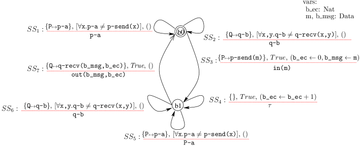
Figure 3. Open automaton for SimpleProtocolSpec

Example

Figure 3 shows the open automaton computed from the SimpleProtocolSpec pNet given in Figure 1. For later references, we name $SS_{i}$ the transitions of this (strong) specification automaton while transitions of the SimpleProtocolImpl pNet are labelled $SI_{i}$. In the figures we annotate each open automaton with the set of its variables.

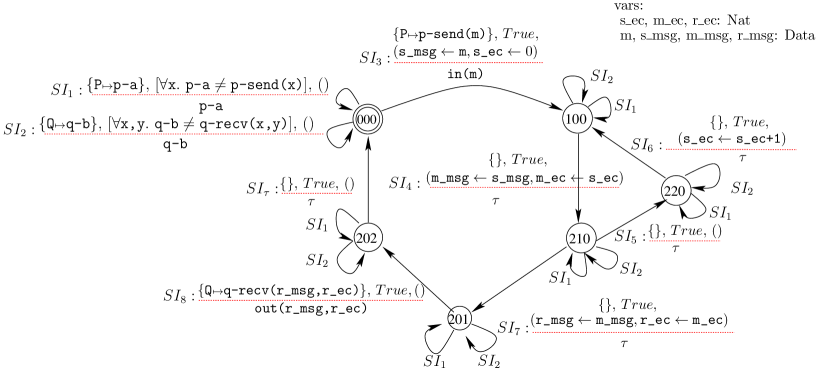
Figure 4. Open automaton for SimpleProtocolImpl

Figure 4 shows the open automaton of SimpleProtocolImpl from Figure 2. In this drawing, we have short labels for states, representing $\triangleleft{s_{0},m_{0},r_{0}}\triangleright$ by 000. Note that open transitions are denoted $\texttt{SI}_{i}$ and tau open transition by $\texttt{SI}_{\tau}$. The resulting behaviour is quite simple: we have a main loop including receiving a message from $P$ and transmitting the same message to $Q$, with some intermediate $\tau$ actions from the internal communications between the protocol processes. In most of the transitions, you can observe that data is propagated between the successive pLTS variables (holding the message, and the error counter value). On the right of the figure, there is a loop of $\tau$ actions ($\texttt{SI}_{4}$, $\texttt{SI}_{5}$ and $\texttt{SI}_{6}$) showing the handling of errors and the incrementation of the error counter.

4.2. pNet Composition Properties: composition of open transitions

The semantics of open pNets allows us to prove two crucial properties relating pNet composition with pNet semantics: open transition of a composed pNet can be decomposed into open transitions of its composing sub-pNets, and conversely, from the open transitions of sub-pNets, an open transition of the composed pNet can be built.

We start with a decomposition property: from one open transition of $P[Q]_{j_{0}}$, we exhibit corresponding behaviours of $P$ and $Q$, and determine the relation between their predicates.

Lemma 3 (Open transition decomposition).

Consider two pNets $P$ and $Q$ that are not pLTSs. Let $\operatorname{Leaves}(Q)=p_{l}^{l\in L_{Q}}$ and suppose:

$$P[Q]_{j_{0}}\models{{\hbox{{\ooalign{\vphantom{$\displaystyle\genfrac{}{}{0.0pt}{0}{\hbox{\hskip 26.96095pt\vbox{\hbox{\hskip-26.96095pt\hbox{\hbox{$\displaystyle\displaystyle\beta_{j}^{j\in J},\makebox{\it Pred},\makebox{\it Post}$}}}\vbox{}}}}{\hbox{\hskip 25.09303pt\vbox{\vbox{}\hbox{\hskip-25.09303pt\hbox{\hbox{$\displaystyle\displaystyle\triangleleft{s_{i}^{i\in L}}\triangleright{\color[rgb]{1,0,0}\,\xrightarrow{{\color[rgb]{0,0,0}\alpha}}\,}\triangleleft{s_{i}^{\prime\,i\in L}}\triangleright$}}}}}}$}\cr{\color[rgb]{1,0,0}\leavevmode\cleaders\hbox to2.20001pt{\raisebox{0.75pt}{\hss$\displaystyle\cdot$\hss}}\hfill\kern 0.0pt}\cr$\displaystyle\genfrac{}{}{0.0pt}{0}{\hbox{\hskip 26.96095pt\vbox{\hbox{\hskip-26.96095pt\hbox{\hbox{$\displaystyle\displaystyle\beta_{j}^{j\in J},\makebox{\it Pred},\makebox{\it Post}$}}}\vbox{}}}}{\hbox{\hskip 25.09303pt\vbox{\vbox{}\hbox{\hskip-25.09303pt\hbox{\hbox{$\displaystyle\displaystyle\triangleleft{s_{i}^{i\in L}}\triangleright{\color[rgb]{1,0,0}\,\xrightarrow{{\color[rgb]{0,0,0}\alpha}}\,}\triangleleft{s_{i}^{\prime\,i\in L}}\triangleright$}}}}}}$\cr}}}}}$$

with $J\cap\operatorname{Holes}(Q)\neq\emptyset$ or $\exists i\in L_{Q}.\,s_{i}\neq s^{\prime}_{i}$, i.e. $Q$ takes part in the reduction. Then there exist $\alpha_{Q}$, $\makebox{\it Pred}\,^{\prime}$, $\makebox{\it Pred}\,^{\prime\prime}$, $\makebox{\it Post}\,^{\prime}$, $\makebox{\it Post}\,^{\prime\prime}$ s.t.:

$$P\models{{\hbox{{\ooalign{\vphantom{$\displaystyle\genfrac{}{}{0.0pt}{0}{\hbox{\hskip 30.16757pt\vbox{\hbox{\hskip-30.16757pt\hbox{\hbox{$\displaystyle\displaystyle\beta_{j}^{j\in(J\setminus\operatorname{Holes}(Q))\cup\{j_{0}\}},\makebox{\it Pred}\,^{\prime},\makebox{\it Post}\,^{\prime}$}}}\vbox{}}}}{\hbox{\hskip 25.09303pt\vbox{\vbox{}\hbox{\hskip-25.09303pt\hbox{\hbox{$\displaystyle\displaystyle\triangleleft{s_{i}^{i\in L\setminus L_{Q}}}\triangleright{\color[rgb]{1,0,0}\,\xrightarrow{{\color[rgb]{0,0,0}\alpha}}\,}\triangleleft{s_{i}^{\prime\,i\in L\setminus L_{Q}}}\triangleright$}}}}}}$}\cr{\color[rgb]{1,0,0}\leavevmode\cleaders\hbox to2.20001pt{\raisebox{0.75pt}{\hss$\displaystyle\cdot$\hss}}\hfill\kern 0.0pt}\cr$\displaystyle\genfrac{}{}{0.0pt}{0}{\hbox{\hskip 30.16757pt\vbox{\hbox{\hskip-30.16757pt\hbox{\hbox{$\displaystyle\displaystyle\beta_{j}^{j\in(J\setminus\operatorname{Holes}(Q))\cup\{j_{0}\}},\makebox{\it Pred}\,^{\prime},\makebox{\it Post}\,^{\prime}$}}}\vbox{}}}}{\hbox{\hskip 25.09303pt\vbox{\vbox{}\hbox{\hskip-25.09303pt\hbox{\hbox{$\displaystyle\displaystyle\triangleleft{s_{i}^{i\in L\setminus L_{Q}}}\triangleright{\color[rgb]{1,0,0}\,\xrightarrow{{\color[rgb]{0,0,0}\alpha}}\,}\triangleleft{s_{i}^{\prime\,i\in L\setminus L_{Q}}}\triangleright$}}}}}}$\cr}}}}}\vspace{-2.2ex}\penalty-10000\hskip 20.00003pt plus 0.5fil minus 5.0pt\text{and~{}\qquad\qquad~{}}Q\models{{\hbox{{\ooalign{\vphantom{$\displaystyle\genfrac{}{}{0.0pt}{0}{\hbox{\hskip 31.70757pt\vbox{\hbox{\hskip-31.70757pt\hbox{\hbox{$\displaystyle\displaystyle\beta_{j}^{j\in J\cap\operatorname{Holes}(Q)},\makebox{\it Pred}\,^{\prime\prime},\makebox{\it Post}\,^{\prime\prime}$}}}\vbox{}}}}{\hbox{\hskip 27.30658pt\vbox{\vbox{}\hbox{\hskip-27.30658pt\hbox{\hbox{$\displaystyle\displaystyle\triangleleft{s_{i}^{i\in L_{Q}}}\triangleright{\color[rgb]{1,0,0}\,\xrightarrow{{\color[rgb]{0,0,0}\alpha_{Q}}}\,}\triangleleft{s_{i}^{\prime\,i\in L_{Q}}}\triangleright$}}}}}}$}\cr{\color[rgb]{1,0,0}\leavevmode\cleaders\hbox to2.20001pt{\raisebox{0.75pt}{\hss$\displaystyle\cdot$\hss}}\hfill\kern 0.0pt}\cr$\displaystyle\genfrac{}{}{0.0pt}{0}{\hbox{\hskip 31.70757pt\vbox{\hbox{\hskip-31.70757pt\hbox{\hbox{$\displaystyle\displaystyle\beta_{j}^{j\in J\cap\operatorname{Holes}(Q)},\makebox{\it Pred}\,^{\prime\prime},\makebox{\it Post}\,^{\prime\prime}$}}}\vbox{}}}}{\hbox{\hskip 27.30658pt\vbox{\vbox{}\hbox{\hskip-27.30658pt\hbox{\hbox{$\displaystyle\displaystyle\triangleleft{s_{i}^{i\in L_{Q}}}\triangleright{\color[rgb]{1,0,0}\,\xrightarrow{{\color[rgb]{0,0,0}\alpha_{Q}}}\,}\triangleleft{s_{i}^{\prime\,i\in L_{Q}}}\triangleright$}}}}}}$\cr}}}}}$$

and $\makebox{\it Pred}\iff\makebox{\it Pred}\,^{\prime}\land\makebox{\it Pred}\,^{\prime\prime}\land\alpha_{Q}=\beta_{j_{0}}$, $\makebox{\it Post}=\makebox{\it Post}\,^{\prime}\uplus\makebox{\it Post}\,^{\prime\prime}$ where $\makebox{\it Post}\,^{\prime\prime}$ is the restriction of Post over variables of $Q$.

Lemma 4 is combining an open transition of $P$ with an open transition of $Q$, and building a corresponding transition of $P[Q]_{j_{0}}$ by assembling their elements.

Lemma 4 (Open transition composition).

Suppose $j_{0}\in J$ and:

$$P\models{{\hbox{{\ooalign{\vphantom{$\displaystyle\genfrac{}{}{0.0pt}{0}{\hbox{\hskip 26.96095pt\vbox{\hbox{\hskip-26.96095pt\hbox{\hbox{$\displaystyle\displaystyle\beta_{j}^{j\in J},\makebox{\it Pred},\makebox{\it Post}$}}}\vbox{}}}}{\hbox{\hskip 25.09303pt\vbox{\vbox{}\hbox{\hskip-25.09303pt\hbox{\hbox{$\displaystyle\displaystyle\triangleleft{s_{i}^{i\in L}}\triangleright{\color[rgb]{1,0,0}\,\xrightarrow{{\color[rgb]{0,0,0}\alpha}}\,}\triangleleft{s_{i}^{\prime\,i\in L}}\triangleright$}}}}}}$}\cr{\color[rgb]{1,0,0}\leavevmode\cleaders\hbox to2.20001pt{\raisebox{0.75pt}{\hss$\displaystyle\cdot$\hss}}\hfill\kern 0.0pt}\cr$\displaystyle\genfrac{}{}{0.0pt}{0}{\hbox{\hskip 26.96095pt\vbox{\hbox{\hskip-26.96095pt\hbox{\hbox{$\displaystyle\displaystyle\beta_{j}^{j\in J},\makebox{\it Pred},\makebox{\it Post}$}}}\vbox{}}}}{\hbox{\hskip 25.09303pt\vbox{\vbox{}\hbox{\hskip-25.09303pt\hbox{\hbox{$\displaystyle\displaystyle\triangleleft{s_{i}^{i\in L}}\triangleright{\color[rgb]{1,0,0}\,\xrightarrow{{\color[rgb]{0,0,0}\alpha}}\,}\triangleleft{s_{i}^{\prime\,i\in L}}\triangleright$}}}}}}$\cr}}}}}\quad\text{~{}~{}and~{}~{}}\quad Q\models{{\hbox{{\ooalign{\vphantom{$\displaystyle\genfrac{}{}{0.0pt}{0}{\hbox{\hskip 30.16757pt\vbox{\hbox{\hskip-30.16757pt\hbox{\hbox{$\displaystyle\displaystyle\beta_{j}^{j\in J_{Q}},\makebox{\it Pred}\,^{\prime},\makebox{\it Post}\,^{\prime}$}}}\vbox{}}}}{\hbox{\hskip 27.30658pt\vbox{\vbox{}\hbox{\hskip-27.30658pt\hbox{\hbox{$\displaystyle\displaystyle\triangleleft{s_{i}^{i\in L_{Q}}}\triangleright{\color[rgb]{1,0,0}\,\xrightarrow{{\color[rgb]{0,0,0}\alpha_{Q}}}\,}\triangleleft{s_{i}^{\prime\,i\in L_{Q}}}\triangleright$}}}}}}$}\cr{\color[rgb]{1,0,0}\leavevmode\cleaders\hbox to2.20001pt{\raisebox{0.75pt}{\hss$\displaystyle\cdot$\hss}}\hfill\kern 0.0pt}\cr$\displaystyle\genfrac{}{}{0.0pt}{0}{\hbox{\hskip 30.16757pt\vbox{\hbox{\hskip-30.16757pt\hbox{\hbox{$\displaystyle\displaystyle\beta_{j}^{j\in J_{Q}},\makebox{\it Pred}\,^{\prime},\makebox{\it Post}\,^{\prime}$}}}\vbox{}}}}{\hbox{\hskip 27.30658pt\vbox{\vbox{}\hbox{\hskip-27.30658pt\hbox{\hbox{$\displaystyle\displaystyle\triangleleft{s_{i}^{i\in L_{Q}}}\triangleright{\color[rgb]{1,0,0}\,\xrightarrow{{\color[rgb]{0,0,0}\alpha_{Q}}}\,}\triangleleft{s_{i}^{\prime\,i\in L_{Q}}}\triangleright$}}}}}}$\cr}}}}}$$

Then, we have:

$$P[Q]_{j_{0}}\models{{\hbox{{\ooalign{\vphantom{$\displaystyle\genfrac{}{}{0.0pt}{0}{\hbox{\hskip 77.36832pt\vbox{\hbox{\hskip-77.36832pt\hbox{\hbox{$\displaystyle\displaystyle\beta_{j}^{(j\in J\setminus\{j_{0}\})\uplus J_{Q}},\makebox{\it Pred}\land\makebox{\it Pred}\,^{\prime}\land\alpha_{Q}=\beta_{j_{0}},\makebox{\it Post}\uplus\makebox{\it Post}\,^{\prime}$}}}\vbox{}}}}{\hbox{\hskip 25.09303pt\vbox{\vbox{}\hbox{\hskip-25.09303pt\hbox{\hbox{$\displaystyle\displaystyle\triangleleft{s_{i}^{i\in L\uplus L_{Q}}}\triangleright{\color[rgb]{1,0,0}\,\xrightarrow{{\color[rgb]{0,0,0}\alpha}}\,}\triangleleft{s_{i}^{\prime\,i\in L\uplus L_{Q}}}\triangleright$}}}}}}$}\cr{\color[rgb]{1,0,0}\leavevmode\cleaders\hbox to2.20001pt{\raisebox{0.75pt}{\hss$\displaystyle\cdot$\hss}}\hfill\kern 0.0pt}\cr$\displaystyle\genfrac{}{}{0.0pt}{0}{\hbox{\hskip 77.36832pt\vbox{\hbox{\hskip-77.36832pt\hbox{\hbox{$\displaystyle\displaystyle\beta_{j}^{(j\in J\setminus\{j_{0}\})\uplus J_{Q}},\makebox{\it Pred}\land\makebox{\it Pred}\,^{\prime}\land\alpha_{Q}=\beta_{j_{0}},\makebox{\it Post}\uplus\makebox{\it Post}\,^{\prime}$}}}\vbox{}}}}{\hbox{\hskip 25.09303pt\vbox{\vbox{}\hbox{\hskip-25.09303pt\hbox{\hbox{$\displaystyle\displaystyle\triangleleft{s_{i}^{i\in L\uplus L_{Q}}}\triangleright{\color[rgb]{1,0,0}\,\xrightarrow{{\color[rgb]{0,0,0}\alpha}}\,}\triangleleft{s_{i}^{\prime\,i\in L\uplus L_{Q}}}\triangleright$}}}}}}$\cr}}}}}$$

Note that this does not mean that any two pNets can be composed and produce an open transition. Indeed, the predicate $\makebox{\it Pred}\land\makebox{\it Pred}\,^{\prime}\land\alpha_{Q}=\beta_{j_{0}}$ is often not satisfiable, in particular if the action $\alpha_{Q}$ cannot be matched with $\beta_{j_{0}}$. Note also that $\beta_{j_{0}}$ is only used as an intermediate term inside formulas in the composed open transition: it does not appear as global action, and will not appear as an action of a hole.

4.3. Bisimulation for open pNets – a composable bisimulation theory

As our symbolic operational semantics provides an open automaton, we can apply the notion of strong (symbolic) bisimulation on automata to open pNets. [FH-bisimulation for open pNets] Two pNets are FH-bisimilar if there exists a relation between their associated automata that is an FH-bisimulation and their initial states are in the relation (i.e. the predicate associated with the initial states is verifiable).

We can now prove that pNet composition preserves FH-bisimulation. More precisely, one can define two preservation properties, namely 1) when one hole of a pNet is filled by two bisimilar other (open) pNets; and 2) when the same hole in two bisimilar pNets are filled by the same pNet, in other words, composing a pNet with two bisimilar contexts. The general case will be obtained by transitivity of the bisimulation relation (Theorem 1).

Theorem 5 (Congruence).

Consider an open pNet: $P=\langle\langle P_{i}^{i\in I},\makebox{\it Sort}_{j}^{j\in J},\overline{\makebox{\it SV}}\rangle\rangle$. Let $j_{0}\in J$ be a hole. Let $Q$ and $Q^{\prime}$ be two FH-bisimilar pNets such that $\operatorname{Sort}(Q)=\operatorname{Sort}(Q^{\prime})=\makebox{\it Sort}_{j_{0}}$. Then $P[Q]_{j_{0}}$ and $P[Q^{\prime}]_{j_{0}}$ are FH-bisimilar.

Theorem 6 (Context equivalence).

Consider two open pNets $P=\langle\langle P_{i}^{i\in I},\makebox{\it Sort}_{j}^{j\in J},\overline{\makebox{\it SV}}\rangle\rangle$ and $P^{\prime}=\langle\langle{P^{\prime}}_{i}^{i\in I},\makebox{\it Sort}_{j}^{j\in J},\overline{\makebox{\it SV'}}\rangle\rangle$ that are FH-bisimilar (recall they must have the same holes to be bisimilar). Let $j_{0}\in J$ be a hole, and $Q$ be a pNet such that $\operatorname{Sort}(Q)=\makebox{\it Sort}_{j_{0}}$. Then $P[Q]_{j_{0}}$ and $P^{\prime}[Q]_{j_{0}}$ are FH-bisimilar.

Finally, the previous theorems can be composed to state a general theorem about composability and FH-bisimilarity.

Theorem 7 (Composability).

Consider two FH-bisimilar pNets with an arbitrary number of holes, when replacing, inside those two original pNets, a subset of the holes by FH-bisimilar pNets, we obtain two FH-bisimilar pNets.

This theorem is quite powerful. It somehow implies that the theory of open pNets is convenient to study properties of process composition. Open pNets can indeed be used to study process operators and process algebras, as shown in [HMZ16] where compositional properties are extremely useful. In the case of interaction protocols [BHHM11], composition of bisimulation can justify abstractions used in some parts of the application.

5. Weak bisimulation

Weak symbolic bisimulation was introduced to relate transition systems that have indistinguishable behaviour, with respect to some definition of internal actions that are considered local to some subsystem, and consequently cannot be observed, nor used for synchronisation with their context. The notion of non-observable actions varies in different contexts, e.g. $tau$ in CCS, and $i$ in Lotos, we could define classically a set of internal/non-observable actions depending on a specific action algebra. In this paper, to simplify the notations, we will simply use $\tau$ as the single non-observable action; the generalisation of our results to a set of non-observable actions is trivial. Naturally, a non-observable action cannot be synchronised with actions of other systems in its environment. We show here that under such assumption of non-observability of $\tau$ actions, see Definition 5.1, we can define a weak bisimulation relation that is compositional, in the sense of open pNet composition. In this section we will first define a notion of weak open transition similar to open transition. In fact a weak open transition is made of several open transitions labelled as non-observable transitions, plus potentially one observable open transition. This allows us to define weak open automata, and a weak bisimulation relation based on these weak open automata. Finally, we apply this weak bisimulation to open pNets, obtain a weak bisimilarity relationship for open pNets, and prove that this relation has compositional properties.

5.1. Preliminary definitions and notations

We first specify in terms of open transition, what it means for an action to be non-observable. Namely, we constraint ourselves to system where the emission of a $\tau$ action by a sub-pNet cannot be observed by the surrounding pNets. In other words, a pNet cannot change its state, or emit a specific observable action when one of its holes emits a $\tau$ action.

More precisely, we state that $\tau$ is not observable if the automaton always allows any $\tau$ transition from holes, and additionally the global transition resulting from a $\tau$ action of a hole is a $\tau$ transition not changing the pNet’s state. We define $\operatorname{Id}(V)$ as the identity function on the set of variables $V$. [Non-observability of $\tau$ actions for open automata] An open automaton $A=\langle\langle J,\mathcal{S},s_{0},V,\mathcal{T}\rangle\rangle$ cannot observe $\tau$ actions if and only if for all $j$ in $J$ and $s$ in $\mathcal{S}$ we have:

1. $${\hbox{{\ooalign{\vphantom{$\displaystyle\genfrac{}{}{0.0pt}{0}{\hbox{\hskip 35.23938pt\vbox{\hbox{\hskip-35.23936pt\hbox{\hbox{$\displaystyle\displaystyle(j\text{\scriptsize{$\displaystyle\mapsto$}}\tau),\makebox{\it True},\operatorname{Id}(V)$}}}\vbox{}}}}{\hbox{\hskip 11.0399pt\vbox{\vbox{}\hbox{\hskip-11.0399pt\hbox{\hbox{$\displaystyle\displaystyle s{\color[rgb]{1,0,0}\,\xrightarrow{{\color[rgb]{0,0,0}\tau}}\,}s$}}}}}}$}\cr{\color[rgb]{1,0,0}\leavevmode\cleaders\hbox to2.20001pt{\raisebox{0.75pt}{\hss$\displaystyle\cdot$\hss}}\hfill\kern 0.0pt}\cr$\displaystyle\genfrac{}{}{0.0pt}{0}{\hbox{\hskip 35.23938pt\vbox{\hbox{\hskip-35.23936pt\hbox{\hbox{$\displaystyle\displaystyle(j\text{\scriptsize{$\displaystyle\mapsto$}}\tau),\makebox{\it True},\operatorname{Id}(V)$}}}\vbox{}}}}{\hbox{\hskip 11.0399pt\vbox{\vbox{}\hbox{\hskip-11.0399pt\hbox{\hbox{$\displaystyle\displaystyle s{\color[rgb]{1,0,0}\,\xrightarrow{{\color[rgb]{0,0,0}\tau}}\,}s$}}}}}}$\cr}}}}\in\mathcal{T}$$

   and

2. for all $\beta_{j}$, $J$, $\alpha$, $s$, $s^{\prime}$, Pred, Post such that

   $${\hbox{{\ooalign{\vphantom{$\displaystyle\genfrac{}{}{0.0pt}{0}{\hbox{\hskip 26.96095pt\vbox{\hbox{\hskip-26.96095pt\hbox{\hbox{$\displaystyle\displaystyle\beta_{j}^{j\in J},\makebox{\it Pred},\makebox{\it Post}$}}}\vbox{}}}}{\hbox{\hskip 12.82265pt\vbox{\vbox{}\hbox{\hskip-12.82263pt\hbox{\hbox{$\displaystyle\displaystyle s{\color[rgb]{1,0,0}\,\xrightarrow{{\color[rgb]{0,0,0}\alpha}}\,}s^{\prime}$}}}}}}$}\cr{\color[rgb]{1,0,0}\leavevmode\cleaders\hbox to2.20001pt{\raisebox{0.75pt}{\hss$\displaystyle\cdot$\hss}}\hfill\kern 0.0pt}\cr$\displaystyle\genfrac{}{}{0.0pt}{0}{\hbox{\hskip 26.96095pt\vbox{\hbox{\hskip-26.96095pt\hbox{\hbox{$\displaystyle\displaystyle\beta_{j}^{j\in J},\makebox{\it Pred},\makebox{\it Post}$}}}\vbox{}}}}{\hbox{\hskip 12.82265pt\vbox{\vbox{}\hbox{\hskip-12.82263pt\hbox{\hbox{$\displaystyle\displaystyle s{\color[rgb]{1,0,0}\,\xrightarrow{{\color[rgb]{0,0,0}\alpha}}\,}s^{\prime}$}}}}}}$\cr}}}}\in\mathcal{T}$$

   If there exists $j$ such that $\beta_{j}=\tau$ then we have:

   $$\alpha=\tau\land s=s^{\prime}\land\makebox{\it Pred}=\makebox{\it True}\land\makebox{\it Post}=\operatorname{Id}(V)\land J=\{j\}$$

The first statement of the definition states that the open automaton must allow a hole to do a silent action at any time, and must not observe it, i.e. it cannot change its internal state because a hole did a $\tau$ transition. The second statement ensures that there cannot be in the open automaton other transitions that would be able to observe a $\tau$ action from a hole: statement (2) states that all the open transitions where a hole does a $\tau$ action must be of the shape given in statement (1). The condition $J=\{j\}$ is a bit restrictive, it could safely be replaced by $\forall j\in J.\,\beta_{j}=\tau$, allowing the other holes to perform $\tau$ transitions too (because these $\tau$ actions cannot be observed).

By definition, one weak open transition contains several open transitions, where each open transition can require an observable action from a given hole, the same hole might have to emit several observable actions for a single weak open transition to occur. Consequently, for a weak open transition to trigger, a sequence of actions from a given hole may be required.

Thus, we let $\gamma$ range over sequences of action terms and use $\mathaccent 0{\cdot}\cup$ as the concatenation operator that appends sequences of action terms: given two sequences of action terms $\gamma\mathaccent 0{\cdot}\cup\gamma^{\prime}$ concatenates the two sequences. The operation is lifted to indexed sets of sequences: at each index $i$, $\overline{\gamma_{1}}\mathaccent 0{\cdot}\cup\overline{\gamma_{2}}$ concatenates the sequences of actions at index $i$ of $\overline{\gamma_{1}}$ and the one at index $i$ of $\overline{\gamma_{2}}$. $[a]$ denotes a sequence with a single element.

As required actions are now sequences of observable actions, we need an operator to build them from set of actions that occur in open transitions, i.e. an operator that takes a set of actions performed by one hole and produces a sequence of observable actions.

Thus we define $(\overline{\beta})^{\nabla}$ as the mapping $\overline{\beta}$ with only observable actions of the holes in $I$, but where each element is either empty or a list of length 1:

$$(\beta_{i}^{i\in I})^{\nabla}=[\beta_{i}]^{i\in I^{\prime}}\text{ where }I^{\prime}=\left\{i|i\in I\land\beta_{i}\neq\tau\right\}$$

As an example the $(\overline{\beta})^{\nabla}$ built from the transition $OT_{1}$ in Example 4.1, page 4.1 is $\texttt{P}\text{\scriptsize{$\mapsto$}}[\texttt{p-send(m)}]$. Remark that in our simple example no $\tau$ transition involves any visible action from a hole, so we have no $\beta$ sequences of length longer than 1 in the weak automaton.

5.2. Weak open transition definition

Because of the non-observability property (Definition 5.1), it is possible to add any number of $\tau$ transitions of the holes before or after any open transition freely. This property justifies the fact that we can abstract away $\tau$ transitions from holes in the definition of a weak open transition. We define weak open transitions similarly to open transitions except that holes can perform sequences of observable actions instead of single actions (observable or not). Compared to the definition of open transition, this small change has a significant impact as a single weak transition is the composition of several transitions of the holes.

[Weak open transition (WOT)] A weak open transition over a set $J$ of holes with sorts $\makebox{\it Sort}_{j}^{j\in J}$ and a set of states $\mathcal{S}$ is a structure of the form:

$$\cdot \genfrac{}{}{0.0pt}{0}{\hbox{\hskip 26.72148pt\vbox{\hbox{\hskip-26.72148pt\hbox{\hbox{$\displaystyle\displaystyle\gamma_{j}^{j\in J^{\prime}},\makebox{\it Pred},\makebox{\it Post}$}}}\vbox{}}}}{\hbox{\hskip 10.32263pt\vbox{\vbox{}\hbox{\hskip-10.32263pt\hbox{\hbox{$\displaystyle\displaystyle s{\color[rgb]{1,0,0}\,\xRightarrow{{\color[rgb]{0,0,0}\alpha}}\,}s^{\prime}$}}}}}}$$

Where $J^{\prime}\subseteq J$, $s,s^{\prime}\in\mathcal{S}$ and $\gamma_{j}$ is a list of transitions of the hole $j$, with each element of the list in $\makebox{\it Sort}_{j}$. $\alpha$ is an action label denoting the resulting action of this open transition. Pred and Post are defined similarly to Definition 3.1. We use $\mathcal{WT}$ to range over sets of weak open transitions.

A weak open automaton $\langle\langle J,\mathcal{S},s_{0},V,\mathcal{WT}\rangle\rangle$ is similar to an open automaton except that $\mathcal{WT}$ is a set of weak open transitions over $J$ and $\mathcal{S}$.

A weak open transition labelled $\alpha$ can be seen as a sequence of open transitions that are all labelled $\tau$ except one that is labelled $\alpha$; however conditions on predicates, effects, and states must be verified for this sequence to be fired.

We are now able to build a weak open automaton from an open automaton. This is done in a way that resembles the process of $\tau$ saturation: we add $\tau$ open transitions before or after another (observable or not) open transition. [Building a weak open automaton] Let $A=\langle\langle J,\mathcal{S},s_{0},V,\mathcal{T}\rangle\rangle$ be an open automaton. The weak open automaton derived from $A$ is an open automaton $\langle\langle J,\mathcal{S},s_{0},V,\mathcal{WT}\rangle\rangle$ where $\mathcal{WT}$ is derived from $\mathcal{T}$ by saturation, applying the following rules:

$${\hbox{{\ooalign{\vphantom{$\displaystyle\genfrac{}{}{0.0pt}{0}{\hbox{\hskip 27.9306pt\vbox{\hbox{\hskip-27.9306pt\hbox{\hbox{$\displaystyle\displaystyle\emptyset,\makebox{\it True},\operatorname{Id}(V)$}}}\vbox{}}}}{\hbox{\hskip 8.5399pt\vbox{\vbox{}\hbox{\hskip-8.53989pt\hbox{\hbox{$\displaystyle\displaystyle s{\color[rgb]{1,0,0}\,\xRightarrow{{\color[rgb]{0,0,0}\tau}}\,}s$}}}}}}$}\cr{\color[rgb]{1,0,0}\leavevmode\cleaders\hbox to2.20001pt{\raisebox{0.75pt}{\hss$\displaystyle\cdot$\hss}}\hfill\kern 0.0pt}\cr$\displaystyle\genfrac{}{}{0.0pt}{0}{\hbox{\hskip 27.9306pt\vbox{\hbox{\hskip-27.9306pt\hbox{\hbox{$\displaystyle\displaystyle\emptyset,\makebox{\it True},\operatorname{Id}(V)$}}}\vbox{}}}}{\hbox{\hskip 8.5399pt\vbox{\vbox{}\hbox{\hskip-8.53989pt\hbox{\hbox{$\displaystyle\displaystyle s{\color[rgb]{1,0,0}\,\xRightarrow{{\color[rgb]{0,0,0}\tau}}\,}s$}}}}}}$\cr}}}}\in\mathcal{WT}\qquad\textbf{WT1}$$

and

$$\displaystyle{\hbox{\hskip 32.26396pt\vbox{\hbox{\hskip-32.26396pt\hbox{\hbox{$\displaystyle\displaystyle{\hbox{{\ooalign{\vphantom{$\displaystyle\genfrac{}{}{0.0pt}{0}{\hbox{\hskip 25.3195pt\vbox{\hbox{\hskip-25.31949pt\hbox{\hbox{$\displaystyle\displaystyle\overline{\beta},\makebox{\it Pred},\makebox{\it Post}$}}}\vbox{}}}}{\hbox{\hskip 12.82265pt\vbox{\vbox{}\hbox{\hskip-12.82263pt\hbox{\hbox{$\displaystyle\displaystyle s{\color[rgb]{1,0,0}\,\xrightarrow{{\color[rgb]{0,0,0}\alpha}}\,}s^{\prime}$}}}}}}$}\cr{\color[rgb]{1,0,0}\leavevmode\cleaders\hbox to2.20001pt{\raisebox{0.75pt}{\hss$\displaystyle\cdot$\hss}}\hfill\kern 0.0pt}\cr$\displaystyle\genfrac{}{}{0.0pt}{0}{\hbox{\hskip 25.3195pt\vbox{\hbox{\hskip-25.31949pt\hbox{\hbox{$\displaystyle\displaystyle\overline{\beta},\makebox{\it Pred},\makebox{\it Post}$}}}\vbox{}}}}{\hbox{\hskip 12.82265pt\vbox{\vbox{}\hbox{\hskip-12.82263pt\hbox{\hbox{$\displaystyle\displaystyle s{\color[rgb]{1,0,0}\,\xrightarrow{{\color[rgb]{0,0,0}\alpha}}\,}s^{\prime}$}}}}}}$\cr}}}}\in\mathcal{T}$}}}\vbox{}}}\over\hbox{\hskip 42.79178pt\vbox{\vbox{}\hbox{\hskip-42.79178pt\hbox{\hbox{$\displaystyle\displaystyle{\hbox{{\ooalign{\vphantom{$\displaystyle\genfrac{}{}{0.0pt}{0}{\hbox{\hskip 30.70842pt\vbox{\hbox{\hskip-30.70842pt\hbox{\hbox{$\displaystyle\displaystyle(\overline{\beta})^{\nabla}\!,\makebox{\it Pred},\makebox{\it Post}$}}}\vbox{}}}}{\hbox{\hskip 10.32263pt\vbox{\vbox{}\hbox{\hskip-10.32263pt\hbox{\hbox{$\displaystyle\displaystyle s{\color[rgb]{1,0,0}\,\xRightarrow{{\color[rgb]{0,0,0}\alpha}}\,}s^{\prime}$}}}}}}$}\cr{\color[rgb]{1,0,0}\leavevmode\cleaders\hbox to2.20001pt{\raisebox{0.75pt}{\hss$\displaystyle\cdot$\hss}}\hfill\kern 0.0pt}\cr$\displaystyle\genfrac{}{}{0.0pt}{0}{\hbox{\hskip 30.70842pt\vbox{\hbox{\hskip-30.70842pt\hbox{\hbox{$\displaystyle\displaystyle(\overline{\beta})^{\nabla}\!,\makebox{\it Pred},\makebox{\it Post}$}}}\vbox{}}}}{\hbox{\hskip 10.32263pt\vbox{\vbox{}\hbox{\hskip-10.32263pt\hbox{\hbox{$\displaystyle\displaystyle s{\color[rgb]{1,0,0}\,\xRightarrow{{\color[rgb]{0,0,0}\alpha}}\,}s^{\prime}$}}}}}}$\cr}}}}\in\mathcal{WT}$}}}}}}$$      WT2

and

$$\displaystyle{\hbox{\hskip 140.60863pt\vbox{\hbox{\hskip-140.60863pt\hbox{\hbox{$\displaystyle\displaystyle{\hbox{{\ooalign{\vphantom{$\displaystyle\genfrac{}{}{0.0pt}{0}{\hbox{\hskip 28.1195pt\vbox{\hbox{\hskip-28.11949pt\hbox{\hbox{$\displaystyle\displaystyle\overline{\gamma_{1}},\makebox{\it Pred}_{1},\makebox{\it Post}_{1}$}}}\vbox{}}}}{\hbox{\hskip 9.9399pt\vbox{\vbox{}\hbox{\hskip-9.9399pt\hbox{\hbox{$\displaystyle\displaystyle s{\color[rgb]{1,0,0}\,\xRightarrow{{\color[rgb]{0,0,0}\tau}}\,}s_{1}$}}}}}}$}\cr{\color[rgb]{1,0,0}\leavevmode\cleaders\hbox to2.20001pt{\raisebox{0.75pt}{\hss$\displaystyle\cdot$\hss}}\hfill\kern 0.0pt}\cr$\displaystyle\genfrac{}{}{0.0pt}{0}{\hbox{\hskip 28.1195pt\vbox{\hbox{\hskip-28.11949pt\hbox{\hbox{$\displaystyle\displaystyle\overline{\gamma_{1}},\makebox{\it Pred}_{1},\makebox{\it Post}_{1}$}}}\vbox{}}}}{\hbox{\hskip 9.9399pt\vbox{\vbox{}\hbox{\hskip-9.9399pt\hbox{\hbox{$\displaystyle\displaystyle s{\color[rgb]{1,0,0}\,\xRightarrow{{\color[rgb]{0,0,0}\tau}}\,}s_{1}$}}}}}}$\cr}}}}\in\mathcal{WT}\qquad{\hbox{{\ooalign{\vphantom{$\displaystyle\genfrac{}{}{0.0pt}{0}{\hbox{\hskip 28.1195pt\vbox{\hbox{\hskip-28.11949pt\hbox{\hbox{$\displaystyle\displaystyle\overline{\gamma_{2}},\makebox{\it Pred}_{2},\makebox{\it Post}_{2}$}}}\vbox{}}}}{\hbox{\hskip 12.35265pt\vbox{\vbox{}\hbox{\hskip-12.35263pt\hbox{\hbox{$\displaystyle\displaystyle s_{1}{\color[rgb]{1,0,0}\,\xRightarrow{{\color[rgb]{0,0,0}\alpha}}\,}s_{2}$}}}}}}$}\cr{\color[rgb]{1,0,0}\leavevmode\cleaders\hbox to2.20001pt{\raisebox{0.75pt}{\hss$\displaystyle\cdot$\hss}}\hfill\kern 0.0pt}\cr$\displaystyle\genfrac{}{}{0.0pt}{0}{\hbox{\hskip 28.1195pt\vbox{\hbox{\hskip-28.11949pt\hbox{\hbox{$\displaystyle\displaystyle\overline{\gamma_{2}},\makebox{\it Pred}_{2},\makebox{\it Post}_{2}$}}}\vbox{}}}}{\hbox{\hskip 12.35265pt\vbox{\vbox{}\hbox{\hskip-12.35263pt\hbox{\hbox{$\displaystyle\displaystyle s_{1}{\color[rgb]{1,0,0}\,\xRightarrow{{\color[rgb]{0,0,0}\alpha}}\,}s_{2}$}}}}}}$\cr}}}}\in\mathcal{WT}\qquad{\hbox{{\ooalign{\vphantom{$\displaystyle\genfrac{}{}{0.0pt}{0}{\hbox{\hskip 28.1195pt\vbox{\hbox{\hskip-28.11949pt\hbox{\hbox{$\displaystyle\displaystyle\overline{\gamma_{3}},\makebox{\it Pred}_{3},\makebox{\it Post}_{3}$}}}\vbox{}}}}{\hbox{\hskip 10.7099pt\vbox{\vbox{}\hbox{\hskip-10.70988pt\hbox{\hbox{$\displaystyle\displaystyle s_{2}{\color[rgb]{1,0,0}\,\xRightarrow{{\color[rgb]{0,0,0}\tau}}\,}s^{\prime}$}}}}}}$}\cr{\color[rgb]{1,0,0}\leavevmode\cleaders\hbox to2.20001pt{\raisebox{0.75pt}{\hss$\displaystyle\cdot$\hss}}\hfill\kern 0.0pt}\cr$\displaystyle\genfrac{}{}{0.0pt}{0}{\hbox{\hskip 28.1195pt\vbox{\hbox{\hskip-28.11949pt\hbox{\hbox{$\displaystyle\displaystyle\overline{\gamma_{3}},\makebox{\it Pred}_{3},\makebox{\it Post}_{3}$}}}\vbox{}}}}{\hbox{\hskip 10.7099pt\vbox{\vbox{}\hbox{\hskip-10.70988pt\hbox{\hbox{$\displaystyle\displaystyle s_{2}{\color[rgb]{1,0,0}\,\xRightarrow{{\color[rgb]{0,0,0}\tau}}\,}s^{\prime}$}}}}}}$\cr}}}}\in\mathcal{WT}$}}}\vbox{\hbox{\hskip-112.21971pt\hbox{\hbox{$\displaystyle\displaystyle\makebox{\it Pred}=\makebox{\it Pred}_{1}\land\makebox{\it Pred}_{2}\{\{\!\makebox{\it Post}_{1}\}\}\land\makebox{\it Pred}_{3}\{\{\!\makebox{\it Post}_{2}\!\odot\!\makebox{\it Post}_{1}\}\}$}}}\vbox{\hbox{\hskip-122.04507pt\hbox{\hbox{$\displaystyle\displaystyle\overline{\gamma}=\overline{\gamma_{1}}\mathaccent 0{\cdot}\cup\overline{\gamma_{2}}\{\{\!\makebox{\it Post}_{1}\}\}\mathaccent 0{\cdot}\cup\overline{\gamma_{3}}\{\{\!\makebox{\it Post}_{2}\!\odot\!\makebox{\it Post}_{1}\}\}$}\hskip 20.00003pt\hbox{\hbox{$\displaystyle\displaystyle\alpha^{\prime}=\alpha\{\{\!\makebox{\it Post}_{1}\}\}$}}}}\vbox{}}}}}\over\hbox{\hskip 69.85289pt\vbox{\vbox{}\hbox{\hskip-69.85289pt\hbox{\hbox{$\displaystyle\displaystyle{\hbox{{\ooalign{\vphantom{$\displaystyle\genfrac{}{}{0.0pt}{0}{\hbox{\hskip 57.76953pt\vbox{\hbox{\hskip-57.76953pt\hbox{\hbox{$\displaystyle\displaystyle\overline{\gamma},\makebox{\it Pred},\makebox{\it Post}_{3}\!\odot\!\makebox{\it Post}_{2}\!\odot\!\makebox{\it Post}_{1}$}}}\vbox{}}}}{\hbox{\hskip 11.09264pt\vbox{\vbox{}\hbox{\hskip-11.09262pt\hbox{\hbox{$\displaystyle\displaystyle s{\color[rgb]{1,0,0}\,\xRightarrow{{\color[rgb]{0,0,0}\alpha^{\prime}}}\,}s^{\prime}$}}}}}}$}\cr{\color[rgb]{1,0,0}\leavevmode\cleaders\hbox to2.20001pt{\raisebox{0.75pt}{\hss$\displaystyle\cdot$\hss}}\hfill\kern 0.0pt}\cr$\displaystyle\genfrac{}{}{0.0pt}{0}{\hbox{\hskip 57.76953pt\vbox{\hbox{\hskip-57.76953pt\hbox{\hbox{$\displaystyle\displaystyle\overline{\gamma},\makebox{\it Pred},\makebox{\it Post}_{3}\!\odot\!\makebox{\it Post}_{2}\!\odot\!\makebox{\it Post}_{1}$}}}\vbox{}}}}{\hbox{\hskip 11.09264pt\vbox{\vbox{}\hbox{\hskip-11.09262pt\hbox{\hbox{$\displaystyle\displaystyle s{\color[rgb]{1,0,0}\,\xRightarrow{{\color[rgb]{0,0,0}\alpha^{\prime}}}\,}s^{\prime}$}}}}}}$\cr}}}}\in\mathcal{WT}$}}}}}}$$WT3

Rule WT1 states that it is always possible to do a non-observable transition, where the state is unchanged and the holes perform no action. Rule WT2 states that each open transition can be considered as a weak open transition. The last rule is the most interesting: Rule WT3 allows any number of $\tau$ transitions before or after any weak open transition. This rules carefully composes predicates, effects, and actions of the holes, indeed in the rule, predicate $\makebox{\it Pred}_{2}$ manipulates variables of $s_{1}$ that result from the first weak open transition. Their values thus depend on the initial state but also on the effect (as a substitution function $\makebox{\it Post}_{1}$) of the first weak open transition. In the same manner, $\makebox{\it Pred}_{3}$ must be applied the substitution defined by the composition $\makebox{\it Post}_{2}\!\odot\!\makebox{\it Post}_{1}$. Similarly, effects on variables must be applied to obtain the global effect of the composed weak open transition, it must also be applied to observable actions of the holes, and to the global action of the weak open transition.

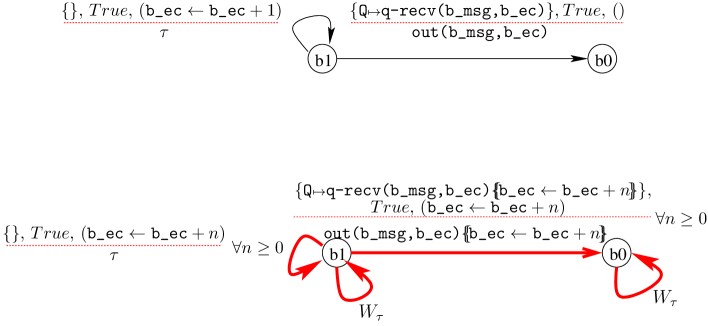
Figure 5. Construction of an example of weak open transition

Example 5.2 (A weak open-transition).

Figure 5 shows the construction of one of the weak transitions of the open automaton of SimpleProtocolSpec. On the top we show the subset of the original open automaton (from Figure 3) considered here, and at the bottom the generated weak transition. For readability, we abbreviate the weak open transitions encoded by $\displaystyle\cdot$ $\displaystyle\genfrac{}{}{0.0pt}{0}{\hbox{\hskip 24.53476pt\vbox{\hbox{\hskip-24.53476pt\hbox{\hbox{$\displaystyle\displaystyle\{\},True,()$}}}\vbox{}}}}{\hbox{\hskip 9.30989pt\vbox{\vbox{}\hbox{\hskip-9.30989pt\hbox{\hbox{$\displaystyle\displaystyle s{\color[rgb]{1,0,0}\,\xRightarrow{{\color[rgb]{0,0,0}\tau}}\,}s^{\prime}$}}}}}}$ as $W_{\tau}$. The weak open transition shown here is the transition delivering the result of the algorithm to hole $Q$ by applying rules: WT1,WT2, and WT3. First rule WT1  adds a $WT_{\tau}$ loop on each state. Rule WT2  transforms each 3 OTs into WOTs. Then consider application of Rule WT3  on a sequence 3 WOTs. $\displaystyle\cdot$ $\displaystyle\genfrac{}{}{0.0pt}{0}{\hbox{\hskip 58.97922pt\vbox{\hbox{\hskip-58.97922pt\hbox{\hbox{$\displaystyle\displaystyle\{\},True,(\texttt{b\_ec}\leftarrow\texttt{b\_ec}+1)$}}}\vbox{}}}}{\hbox{\hskip 14.40799pt\vbox{\vbox{}\hbox{\hskip-14.40797pt\hbox{\hbox{$\displaystyle\displaystyle\texttt{b1}{\color[rgb]{1,0,0}\,\xRightarrow{{\color[rgb]{0,0,0}\tau}}\,}\texttt{b1}$}}}}}}$ ; $\displaystyle\cdot$ $\displaystyle\genfrac{}{}{0.0pt}{0}{\hbox{\hskip 58.97922pt\vbox{\hbox{\hskip-58.97922pt\hbox{\hbox{$\displaystyle\displaystyle\{\},True,(\texttt{b\_ec}\leftarrow\texttt{b\_ec}+1)$}}}\vbox{}}}}{\hbox{\hskip 14.40799pt\vbox{\vbox{}\hbox{\hskip-14.40797pt\hbox{\hbox{$\displaystyle\displaystyle\texttt{b1}{\color[rgb]{1,0,0}\,\xRightarrow{{\color[rgb]{0,0,0}\tau}}\,}\texttt{b1}$}}}}}}$ ; $\displaystyle\cdot$ $\displaystyle\genfrac{}{}{0.0pt}{0}{\hbox{\hskip 24.53476pt\vbox{\hbox{\hskip-24.53476pt\hbox{\hbox{$\displaystyle\displaystyle\{\},True,()$}}}\vbox{}}}}{\hbox{\hskip 14.40799pt\vbox{\vbox{}\hbox{\hskip-14.40797pt\hbox{\hbox{$\displaystyle\displaystyle\texttt{b1}{\color[rgb]{1,0,0}\,\xRightarrow{{\color[rgb]{0,0,0}\tau}}\,}\texttt{b1}$}}}}}}$ . The result will be: $\displaystyle\cdot$ $\displaystyle\genfrac{}{}{0.0pt}{0}{\hbox{\hskip 58.97922pt\vbox{\hbox{\hskip-58.97922pt\hbox{\hbox{$\displaystyle\displaystyle\{\},True,(\texttt{b\_ec}\leftarrow\texttt{b\_ec}+2)$}}}\vbox{}}}}{\hbox{\hskip 14.40799pt\vbox{\vbox{}\hbox{\hskip-14.40797pt\hbox{\hbox{$\displaystyle\displaystyle\texttt{b1}{\color[rgb]{1,0,0}\,\xRightarrow{{\color[rgb]{0,0,0}\tau}}\,}\texttt{b1}$}}}}}}$ . We can iterate this construction an arbitrary number of times, getting for any natural number $n$ a weak open transition: ${\hbox{{\ooalign{\vphantom{$\displaystyle\genfrac{}{}{0.0pt}{0}{\hbox{\hskip 43.9248pt\vbox{\hbox{\hskip-43.9248pt\hbox{\hbox{$\displaystyle\displaystyle\emptyset,True,(\texttt{ec}\leftarrow\texttt{ec}+n)$}}}\vbox{}}}}{\hbox{\hskip 14.40799pt\vbox{\vbox{}\hbox{\hskip-14.40797pt\hbox{\hbox{$\displaystyle\displaystyle\texttt{b1}{\color[rgb]{1,0,0}\,\xRightarrow{{\color[rgb]{0,0,0}\tau}}\,}\texttt{b1}$}}}}}}$}\cr{\color[rgb]{1,0,0}\leavevmode\cleaders\hbox to2.20001pt{\raisebox{0.75pt}{\hss$\displaystyle\cdot$\hss}}\hfill\kern 0.0pt}\cr$\displaystyle\genfrac{}{}{0.0pt}{0}{\hbox{\hskip 43.9248pt\vbox{\hbox{\hskip-43.9248pt\hbox{\hbox{$\displaystyle\displaystyle\emptyset,True,(\texttt{ec}\leftarrow\texttt{ec}+n)$}}}\vbox{}}}}{\hbox{\hskip 14.40799pt\vbox{\vbox{}\hbox{\hskip-14.40797pt\hbox{\hbox{$\displaystyle\displaystyle\texttt{b1}{\color[rgb]{1,0,0}\,\xRightarrow{{\color[rgb]{0,0,0}\tau}}\,}\texttt{b1}$}}}}}}$\cr}}}}\,\forall n\geq 0$. Finally, applying again WT3, and using the central open transition having out(b_msg,b_ec) as $\alpha$, we get the resulting weak open transition between b1 and b0 (as shown in Figure 5). Applying the substitutions finally yields the weak transitions family $WS_{7}$ in Figure 6.

Example 5.3 (Weak open automata).

Figures 6 and 7 respectively show the weak automata of SimpleProtocolSpec and SimpleProtocolImpl. We encode weak open transitions by $WS$ on the specification model and by $WI$ on the implementation model.

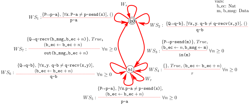
Figure 6. Weak Open Automaton of SimpleProtocolSpec

For readability, we only give names to the weak open transitions of SimpleProtocolImpl in Figure 7; we detail some of these transitions below and the full list is included in Appendix LABEL:Appendix:FullExample. Let us point out that the weak OT loops ($WI_{1}$,$WI_{2}$ and $W_{\tau}$) on state ${000}$ are also present in all other states, we did not repeat them. Additionally, many WOTs are similar, and numbered accordingly as 3, 3a, 3b, 3c and 8, 8a, 8b, 8c respectively: they only differ by their respective source or target states; the "variant" WOTs appear in blue in Figure 7.

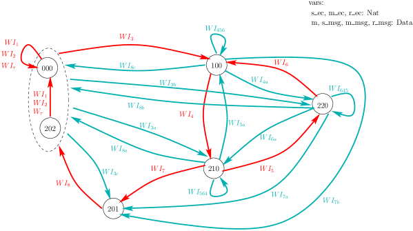
Figure 7. Weak Open Automaton of SimpleProtocolImpl

Now let us give some details about the construction of the weak automaton of the SimpleProtocolImpl pNet, obtained by application of the weak rules as explained above. We concentrate on weak open transitions $WI_{3}$ and $WI_{4}$. Let us denote as $post_{n}$ the effect (as a substitution function) of the strong open transitions $SI_{n}$ from Figure 4:

$post_{3}=(\texttt{s\_msg}\leftarrow\texttt{m},\texttt{s\_ec}\leftarrow 0)$

$post_{4}=(\texttt{m\_msg}\leftarrow\texttt{s\_msg},\texttt{m\_ec}\leftarrow\texttt{s\_ec})$

$post_{5}=()$

$post_{6}=(\texttt{s\_ec}\leftarrow\texttt{s\_ec+1})$

Then the effect of one single $100\xrightarrow{OT_{4}}210\xrightarrow{OT_{5}}220\xrightarrow{OT_{6}}100$ loop is:

$$post_{456}=post_{6}\!\odot\!\ post_{5}\!\odot\!\ post_{4}=(\texttt{s\_ec}\leftarrow\texttt{s\_ec}+1)$$

So if we denote ${post_{456*}}$ any iteration of this loop, we get ${post_{456*}}=(\texttt{s\_ec}\leftarrow\texttt{s\_ec}+n)$ for any $n\geq 0$, and the Post  of the weak OT $WI_{3}$ is:
$Post_{3}=post_{456*}\!\odot\!\ post_{3}=(\texttt{s\_msg}\leftarrow m,\texttt{s\_ec}\leftarrow n),\forall n\geq 0$ and Post  of $WI_{3a}$ is:
$post_{4}\!\odot\!{post_{456*}}\!\odot\!\ post_{3}=(\texttt{m\_msg}\leftarrow m,\texttt{m\_ec}\leftarrow n),\forall n\geq 0$.

We can now show some of the weak OTs of Figure 7 (the full table is included in Appendix LABEL:Appendix:FullExample). As we have seen above, the effect of rule $WT_{3}$ when a silent action have an effect on the variable $ec$ will generate an infinite family of WOTs, depending on the number of iterations through the loops. We denote these families using a "meta-variable" $n$, ranging over Nat.

$WI_{1}={\hbox{{\ooalign{\vphantom{$\displaystyle\genfrac{}{}{0.0pt}{0}{\hbox{\hskip 66.06953pt\vbox{\hbox{\hskip-66.06952pt\hbox{\hbox{$\displaystyle\displaystyle\{\texttt{P}\text{\scriptsize{$\displaystyle\mapsto$}}\texttt{p-a}\},[\forall\texttt{x}.\texttt{p-a}\neq\texttt{p-send(x)}],()$}}}\vbox{}}}}{\hbox{\hskip 13.29858pt\vbox{\vbox{}\hbox{\hskip-13.29858pt\hbox{\hbox{$\displaystyle\displaystyle s{\color[rgb]{1,0,0}\,\xRightarrow{{\color[rgb]{0,0,0}\texttt{p-a}}}\,}s$}}}}}}$}\cr{\color[rgb]{1,0,0}\leavevmode\cleaders\hbox to2.20001pt{\raisebox{0.75pt}{\hss$\displaystyle\cdot$\hss}}\hfill\kern 0.0pt}\cr$\displaystyle\genfrac{}{}{0.0pt}{0}{\hbox{\hskip 66.06953pt\vbox{\hbox{\hskip-66.06952pt\hbox{\hbox{$\displaystyle\displaystyle\{\texttt{P}\text{\scriptsize{$\displaystyle\mapsto$}}\texttt{p-a}\},[\forall\texttt{x}.\texttt{p-a}\neq\texttt{p-send(x)}],()$}}}\vbox{}}}}{\hbox{\hskip 13.29858pt\vbox{\vbox{}\hbox{\hskip-13.29858pt\hbox{\hbox{$\displaystyle\displaystyle s{\color[rgb]{1,0,0}\,\xRightarrow{{\color[rgb]{0,0,0}\texttt{p-a}}}\,}s$}}}}}}$\cr}}}}$ (for any $s\in S$)

$\forall n\geq 0.\,WI_{3}(n)={\hbox{{\ooalign{\vphantom{$\displaystyle\genfrac{}{}{0.0pt}{0}{\hbox{\hskip 96.04987pt\vbox{\hbox{\hskip-96.04987pt\hbox{\hbox{$\displaystyle\displaystyle\{\texttt{P}\text{\scriptsize{$\displaystyle\mapsto$}}\texttt{p-send(m)}\},True,(\texttt{s\_msg}\leftarrow\texttt{m},\texttt{s\_ec}\leftarrow n)$}}}\vbox{}}}}{\hbox{\hskip 28.88893pt\vbox{\vbox{}\hbox{\hskip-28.88893pt\hbox{\hbox{$\displaystyle\displaystyle 000{\color[rgb]{1,0,0}\,\xRightarrow{{\color[rgb]{0,0,0}\texttt{in(m)}}}\,}100$}}}}}}$}\cr{\color[rgb]{1,0,0}\leavevmode\cleaders\hbox to2.20001pt{\raisebox{0.75pt}{\hss$\displaystyle\cdot$\hss}}\hfill\kern 0.0pt}\cr$\displaystyle\genfrac{}{}{0.0pt}{0}{\hbox{\hskip 96.04987pt\vbox{\hbox{\hskip-96.04987pt\hbox{\hbox{$\displaystyle\displaystyle\{\texttt{P}\text{\scriptsize{$\displaystyle\mapsto$}}\texttt{p-send(m)}\},True,(\texttt{s\_msg}\leftarrow\texttt{m},\texttt{s\_ec}\leftarrow n)$}}}\vbox{}}}}{\hbox{\hskip 28.88893pt\vbox{\vbox{}\hbox{\hskip-28.88893pt\hbox{\hbox{$\displaystyle\displaystyle 000{\color[rgb]{1,0,0}\,\xRightarrow{{\color[rgb]{0,0,0}\texttt{in(m)}}}\,}100$}}}}}}$\cr}}}}$

$\forall n\geq 0.\,WI_{4}(n)={\hbox{{\ooalign{\vphantom{$\displaystyle\genfrac{}{}{0.0pt}{0}{\hbox{\hskip 135.42598pt\vbox{\hbox{\hskip-135.42596pt\hbox{\hbox{$\displaystyle\displaystyle\{\},True,(\texttt{m\_msg}\!\leftarrow\!\texttt{s\_msg},\texttt{m\_ec}\!\leftarrow\!\texttt{s\_ec}+n,\texttt{s\_ec}\!\leftarrow\!\texttt{s\_ec}+n)$}}}\vbox{}}}}{\hbox{\hskip 18.85245pt\vbox{\vbox{}\hbox{\hskip-18.85243pt\hbox{\hbox{$\displaystyle\displaystyle 100{\color[rgb]{1,0,0}\,\xRightarrow{{\color[rgb]{0,0,0}\tau}}\,}210$}}}}}}$}\cr{\color[rgb]{1,0,0}\leavevmode\cleaders\hbox to2.20001pt{\raisebox{0.75pt}{\hss$\displaystyle\cdot$\hss}}\hfill\kern 0.0pt}\cr$\displaystyle\genfrac{}{}{0.0pt}{0}{\hbox{\hskip 135.42598pt\vbox{\hbox{\hskip-135.42596pt\hbox{\hbox{$\displaystyle\displaystyle\{\},True,(\texttt{m\_msg}\!\leftarrow\!\texttt{s\_msg},\texttt{m\_ec}\!\leftarrow\!\texttt{s\_ec}+n,\texttt{s\_ec}\!\leftarrow\!\texttt{s\_ec}+n)$}}}\vbox{}}}}{\hbox{\hskip 18.85245pt\vbox{\vbox{}\hbox{\hskip-18.85243pt\hbox{\hbox{$\displaystyle\displaystyle 100{\color[rgb]{1,0,0}\,\xRightarrow{{\color[rgb]{0,0,0}\tau}}\,}210$}}}}}}$\cr}}}}$

$\forall n\geq 0.\,WI_{456}(n)={\hbox{{\ooalign{\vphantom{$\displaystyle\genfrac{}{}{0.0pt}{0}{\hbox{\hskip 57.86926pt\vbox{\hbox{\hskip-57.86925pt\hbox{\hbox{$\displaystyle\displaystyle\{\},True,(\texttt{s\_ec}\leftarrow\texttt{s\_ec}+n)$}}}\vbox{}}}}{\hbox{\hskip 18.85245pt\vbox{\vbox{}\hbox{\hskip-18.85243pt\hbox{\hbox{$\displaystyle\displaystyle 100{\color[rgb]{1,0,0}\,\xRightarrow{{\color[rgb]{0,0,0}\tau}}\,}100$}}}}}}$}\cr{\color[rgb]{1,0,0}\leavevmode\cleaders\hbox to2.20001pt{\raisebox{0.75pt}{\hss$\displaystyle\cdot$\hss}}\hfill\kern 0.0pt}\cr$\displaystyle\genfrac{}{}{0.0pt}{0}{\hbox{\hskip 57.86926pt\vbox{\hbox{\hskip-57.86925pt\hbox{\hbox{$\displaystyle\displaystyle\{\},True,(\texttt{s\_ec}\leftarrow\texttt{s\_ec}+n)$}}}\vbox{}}}}{\hbox{\hskip 18.85245pt\vbox{\vbox{}\hbox{\hskip-18.85243pt\hbox{\hbox{$\displaystyle\displaystyle 100{\color[rgb]{1,0,0}\,\xRightarrow{{\color[rgb]{0,0,0}\tau}}\,}100$}}}}}}$\cr}}}}$

The Post of the weak OT $WI_{6a}$ is:

$$\begin{array}[]{l@{}l}Post_{6a}&=post_{4}\!\odot\!\ post_{456*}\!\odot\!\ post_{6}\\ &=(\texttt{m\_msg}\leftarrow\texttt{s\_msg},\texttt{m\_ec}\leftarrow\texttt{s\_ec})\,\!\odot\!(\texttt{s\_ec}\leftarrow\texttt{s\_ec}+n)\!\odot\!(\texttt{s\_ec}\leftarrow\texttt{s\_ec}+1)\\ &=(\texttt{m\_msg}\!\leftarrow\texttt{s\_msg},\texttt{m\_ec}\!\leftarrow\texttt{s\_ec}+1\!+\!n,\texttt{s\_ec}\!\leftarrow\texttt{s\_ec}+1\!+\!n)\end{array}$$

So we get:

$\forall n\geq 0.\,WI_{6a}(n)={\hbox{{\ooalign{\vphantom{$\displaystyle\genfrac{}{}{0.0pt}{0}{\hbox{\hskip 112.00926pt\vbox{\hbox{\hskip-112.00925pt\hbox{\hbox{$\displaystyle\displaystyle\{\},True,(\texttt{m\_ec}\leftarrow\texttt{s\_ec}+1+n,\texttt{s\_ec}\leftarrow\texttt{s\_ec}+1+n)$}}}\vbox{}}}}{\hbox{\hskip 18.85245pt\vbox{\vbox{}\hbox{\hskip-18.85243pt\hbox{\hbox{$\displaystyle\displaystyle 220{\color[rgb]{1,0,0}\,\xRightarrow{{\color[rgb]{0,0,0}\tau}}\,}210$}}}}}}$}\cr{\color[rgb]{1,0,0}\leavevmode\cleaders\hbox to2.20001pt{\raisebox{0.75pt}{\hss$\displaystyle\cdot$\hss}}\hfill\kern 0.0pt}\cr$\displaystyle\genfrac{}{}{0.0pt}{0}{\hbox{\hskip 112.00926pt\vbox{\hbox{\hskip-112.00925pt\hbox{\hbox{$\displaystyle\displaystyle\{\},True,(\texttt{m\_ec}\leftarrow\texttt{s\_ec}+1+n,\texttt{s\_ec}\leftarrow\texttt{s\_ec}+1+n)$}}}\vbox{}}}}{\hbox{\hskip 18.85245pt\vbox{\vbox{}\hbox{\hskip-18.85243pt\hbox{\hbox{$\displaystyle\displaystyle 220{\color[rgb]{1,0,0}\,\xRightarrow{{\color[rgb]{0,0,0}\tau}}\,}210$}}}}}}$\cr}}}}$

5.3. Composition properties: composition of weak open transitions

We now have two different semantics for open pNets: a strong semantics, defined as an open automaton, and as a weak semantics, defined as a weak open automaton. Like the open automaton, the weak open automaton features valuable composition properties. We can exhibit a composition property and a decomposition property that relate open pNet composition with their semantics, defined as weak open automata. These are however technically more complex than the ones for open automata because each hole performs a set of actions, and thus a composed transition is the composition of one transition of the top-level pNet and a sequence of transitions of the sub-pNet that fills its hole. They can be found as Lemmas LABEL:lem-decomposeWOT, Lemma LABEL:lem-Weakcompose1, and Lemma LABEL:lem-Weakcompose in Appendix LABEL:sec:app-composition.

5.4. Weak FH-bisimulation

For defining a bisimulation relation between weak open automata, two options are possible. Either we define a simulation similar to the strong simulation but based on open automata, this would look like the FH-simulation but would need to be adapted to weak open transitions. Or we define directly and classically a weak FH-simulation as a relation between two open automata, relating the open transition of the first one with the transition of the weak open automaton derived from the second one.

The definition below specifies how a set of weak open transitions can simulate an open transition, and under which condition; this is used to relate, by weak FH-bisimulation, two open automata by reasoning on the weak open automata that can be derived from the strong ones. This is defined formally as follows.

[Weak FH-bisimulation]  
Let $A_{1}=\langle\langle J,\mathcal{S}_{1},s_{0},V_{1},\mathcal{T}_{1}\rangle\rangle$ and $A_{2}=\langle\langle J,\mathcal{S}_{2},t_{0},V_{2},\mathcal{T}_{2}\rangle\rangle$ be open automata with disjoint sets of variables. Let $\langle\langle J,\mathcal{S}_{1},s_{0},V_{1},\mathcal{WT}_{1}\rangle\rangle$ and $\langle\langle J,\mathcal{S}_{2},t_{0},V_{2},\mathcal{WT}_{2}\rangle\rangle$ be the weak open automata derived from $A_{1}$ and $A_{2}$ respectively. Let $\mathcal{R}$ a relation over $\mathcal{S}_{1}$ and $\mathcal{S}_{2}$, as in Definition 3.

Then $\mathcal{R}$ is a weak FH-bisimulation iff for any states $s\in\mathcal{S}_{1}$ and $t\in\mathcal{S}_{2}$ such that $(s,t|\makebox{\it Pred}_{s,t})\in\mathcal{R}$, we have the following:

• For any open transition $OT$ in $\mathcal{T}_{1}$:

  $$\cdot \genfrac{}{}{0.0pt}{0}{\hbox{\hskip 35.43834pt\vbox{\hbox{\hskip-35.43834pt\hbox{\hbox{$\displaystyle\displaystyle\beta_{j}^{j\in J^{\prime}},\makebox{\it Pred}_{OT},\makebox{\it Post}_{OT}$}}}\vbox{}}}}{\hbox{\hskip 12.82265pt\vbox{\vbox{}\hbox{\hskip-12.82263pt\hbox{\hbox{$\displaystyle\displaystyle s{\color[rgb]{1,0,0}\,\xrightarrow{{\color[rgb]{0,0,0}\alpha}}\,}s^{\prime}$}}}}}}$$

  there exists an indexed set of weak open transitions $\makebox{\it WOT}_{x}^{\;x\in X}\subseteq\mathcal{WT}_{2}$:

  $$\cdot \genfrac{}{}{0.0pt}{0}{\hbox{\hskip 38.62802pt\vbox{\hbox{\hskip-38.628pt\hbox{\hbox{$\displaystyle\displaystyle\gamma_{jx}^{j\in J_{x}},\makebox{\it Pred}_{OT_{x}},\makebox{\it Post}_{OT_{x}}$}}}\vbox{}}}}{\hbox{\hskip 11.6768pt\vbox{\vbox{}\hbox{\hskip-11.67679pt\hbox{\hbox{$\displaystyle\displaystyle t{\color[rgb]{1,0,0}\,\xRightarrow{{\color[rgb]{0,0,0}\alpha_{x}}}\,}t_{x}$}}}}}}$$

  such that $\forall x.\,\{j\in J^{\prime}|\beta_{j}\neq\tau\}=J_{x},(s^{\prime},t_{x}|\makebox{\it Pred}_{s^{\prime},t_{x}})\in\mathcal{R}$; and

  $$\makebox{\it Pred}_{s,t}\land\makebox{\it Pred}_{OT}\\ \hskip 28.45274pt\implies\!\!\!\displaystyle{\bigvee_{x\in X}\!\left(\forall j\in J_{x}.(\beta_{j})^{\nabla}\!=\!\gamma_{jx}\!\land\!\makebox{\it Pred}_{OT_{x}}\!\land\!\alpha\!=\!\alpha_{x}\!\land\!\makebox{\it Pred}_{s^{\prime},t_{x}}\{\{\!\makebox{\it Post}_{OT}\uplus\makebox{\it Post}_{OT_{x}}\}\}\right)}$$

• and symmetrically any open transition from $t$ in $\mathcal{T}_{2}$ can be covered by a set of weak transitions from $s$ in $\mathcal{WT}_{1}$.

Two pNets are weak FH-bisimilar if there exists a relation between their associated automata that is a weak FH-bisimulation and their initial states are in the relation, i.e. the predicate associated to the relation between the initial states is True.

Compared to strong bisimulation, except the obvious use of weak open transitions to simulate an open transition, the condition on predicate is slightly changed concerning actions of the holes. Indeed only the visible actions of the holes must be compared and they form a list of actions, but of length at most one.

Our first important result is that weak FH-bisimilarity is an equivalence in the same way as strong FH-bisimilarity:

Theorem 8 (Weak FH-Bisimulation is an equivalence).

Suppose $\mathcal{R}$ is a weak FH-bisimulation. Then $\mathcal{R}$ is an equivalence, that is, $\mathcal{R}$ is reflexive, symmetric and transitive.

The proof is detailed in Appendix LABEL:app-WFH-equiv, it follows a similar pattern as the proof that strong FH-bisimulation is an equivalence, but technical details are different, and in practice we rely on a variant of the definition of weak FH-bisimilarity; this equivalent version simulates a weak open transition with a set of weak open transition. The careful use of the best definition of weak FH-bisimilarity makes the proof similar to the strong FH-bisimulation case.

Proving bisimulation in practice

In practice, we are dealing with finite representations of the (infinite) open automata. In [HM20], we defined a slightly modified definition of the “coverage” proof obligation, in the case of strong FH-Bisimulation. This modification is required to manage in a finite way all possible instantiations of an OT. In the case of weak FH-Bisimulation, the proof obligation from Definition 5.4 becomes:

$$\forall fv_{OT}.\,\Big{\{}\makebox{\it Pred}_{s,t}\land\makebox{\it Pred}_{OT}\implies\\ \bigvee_{x\in X}\!\left[\exists fv_{OT_{x}}.\left(\forall j\in J_{x}.(\beta_{j})^{\nabla}\!=\!\gamma_{jx}\!\land\!\makebox{\it Pred}_{OT_{x}}\!\land\!\alpha\!=\!\alpha_{x}\!\land\!\makebox{\it Pred}_{s^{\prime},t_{x}}\{\{\!\makebox{\it Post}_{OT}\uplus\makebox{\it Post}_{OT_{x}}\}\}\right)\right]\Big{\}}$$

where $fv_{OT}$ denotes the set of free variables of all expressions in $OT$.

5.5. Weak bisimulation for open pNets

Before defining a weak open automaton for the semantics of open pNets, it is necessary to state under which condition a pNet is unable to observe silent actions of its holes. In the setting of pNets this can simply be expressed as a condition on the synchronisation vectors. Precisely, the set of synchronisation vectors must contain vectors that let silent actions go through the pNet, i.e. synchronisation vectors where one hole does a $\tau$ transition, and the global visible action is a $\tau$. Additionally, no other synchronisation vector must be able to react on a silent action from a hole, i.e. if a synchronisation vector observes a $\tau$ from a hole it cannot synchronise it with another action nor emit an action that is not $\tau$. This is formalised as follows:

[Non-observability of silent actions for pNets] 
A pNet $\langle\langle P_{i}^{i\in I},\makebox{\it Sort}_{j}^{j\in J},\overline{\makebox{\it SV}}\rangle\rangle$ cannot observe silent actions if it verifies:
$\forall i\in I\uplus J.\,(i\text{\scriptsize{$\mapsto$}}\tau)\to\tau[\makebox{\it True}]\in\overline{\makebox{\it SV}}$ and

$$\forall\left({(\alpha_{i})}^{i\in I^{\prime}}\to\alpha^{\prime}[e_{b}]\in\overline{\makebox{\it SV}}\right),\forall i\in I^{\prime}\cap J.\,\alpha_{i}=\tau\implies\alpha^{\prime}=\tau~{}\land~{}I^{\prime}=\{i\}$$

Example 5.4 (CCS choice (counter-example)).

Here is the encoding of a choice operator.
The left hole is indexed $l$ the right hole $r$. The third subnet, contains an LTS encoding the control part. We obtain the specific behaviour with the synchronisation vector. The first action of one of the holes decides which branch of the LTS is activated; all subsequent actions will be from the same side.

This pNet does not satisfy Definition 5.5. Indeed, if $a$ or $b$ is $\tau$ then the $+$ operator can indeed observe the $\tau$ transition. On the other side, the parallel operator defined similarly satisfies Definition 5.5.

With this definition, it is easy to check that the open automaton that gives the semantics of such an open pNet cannot observe silent actions in the sense of Definition 5.1.

Property 1 (Non-observability of silent actions).

The semantics of a pNet, as provided in Definition 4.1, that cannot observe silent actions is an open automaton that cannot observe silent actions.

Under this condition, it is safe to define the weak open automaton that provides a weak semantics to a given pNet. This is simply obtained by applying Definition 5.2 to generate a weak open automaton from the open automaton that is the strong semantics of the open pNet, as provided by Definition 4.1.

[Semantics of pNets as a weak open automaton] Let $A$ be the open automaton expressing the semantics of an open pNet $P$; let $\langle\langle J,\mathcal{S},s_{0},V,\mathcal{WT}\rangle\rangle$ be the weak open automaton derived from $A$; we call this weak open automaton the weak semantics of the pNet $P$. Then, we denote $P\models\makebox{\it WOT}$ whenever $\makebox{\it WOT}\in\mathcal{WT}$.

From the definition of the weak open automata of pNets, we can now study the properties of weak bisimulation concerning open pNets.

5.6. Properties of weak bisimulation for open pNets

When silent actions cannot be observed, weak bisimulation is a congruence for open pNets: if $P$ and $Q$ are weakly bisimilar to $P^{\prime}$ and $Q^{\prime}$ then the composition of $P$ and $Q$ is weakly bisimilar to the composition of $P^{\prime}$ and $Q^{\prime}$, where composition is the hole replacement operator: $P[Q]_{j}$ and $P^{\prime}[Q^{\prime}]_{j}$ are weak FH-bisimilar. This can be shown by proving the two following theorems. The detailed proof of these theorem can be found in Appendix LABEL:sec:app-composition. The proof strongly relies on the fact that weak FH-bisimulation is an equivalence, but also on the composition properties for open automata.

Theorem 9 (Congruence for weak bisimulation).

Consider an open pNet $P$ that cannot observe silent actions, of the form $P=\langle\langle P_{i}^{i\in I},\makebox{\it Sort}_{j}^{j\in J},\overline{\makebox{\it SV}}\rangle\rangle$. Let $j_{0}\in J$ be a hole. Let $Q$ and $Q^{\prime}$ be two weak FH-bisimilar pNets such that $\operatorname{Sort}(Q)=\operatorname{Sort}(Q^{\prime})\subseteq\makebox{\it Sort}_{j_{0}}$. Then $P[Q]_{j_{0}}$ and $P[Q^{\prime}]_{j_{0}}$ are weak FH-bisimilar.

Theorem 10 (Context equivalence for weak bisimulation).

Consider two open pNets $P=\langle\langle P_{i}^{i\in I},\makebox{\it Sort}_{j}^{j\in J},\overline{\makebox{\it SV}}\rangle\rangle$ and $P^{\prime}=\langle\langle{P^{\prime}}_{i}^{i\in I},\makebox{\it Sort}_{j}^{j\in J},\overline{\makebox{\it SV'}}\rangle\rangle$ that are weak FH-bisimilar (recall they must have the same holes to be bisimilar) and that cannot observe silent actions. Let $j_{0}\in J$ be a hole, and $Q$ be a pNet such that $\operatorname{Sort}(Q)\subseteq\makebox{\it Sort}_{j_{0}}$. Then $P[Q]_{j_{0}}$ and $P^{\prime}[Q]_{j_{0}}$ are weak FH-bisimilar.

Finally, the previous theorems can be composed to state a general theorem about composability and weak FH-bisimilarity.

Theorem 11 (Composability of weak bisimulation).

Consider two weak FH-bisimilar pNets with an arbitrary number of holes, such that the two pNets cannot observe silent actions. When replacing, inside those two original pNets, a subset of the holes by weak FH-bisimilar pNets, we obtain two weak FH-bisimilar pNets.

Example 5.5 (CCS Choice).

Consider the $+$ operator of CCS, shown in Example 5.4. It is well-known that weak bisimulation is not a congruence in CCS, and this is reflected here because we have shown that the $+$ operator can observe the $\tau$ transitions. Thus, even if we can define a weak bisimulation for CCS with $+$ it does not verify the necessary requirements for being a congruence.

Running example

In Section 5 we have shown the full saturated weak automaton for both SimpleProtocolSpec and SimpleProtocolImpl. We will show here how we can check if some given relation between these two automata is a weak FH-Bisimulation.

Preliminary remarks:

• Both pNets trivially verify the “non-observability” condition: the only vectors having $\tau$ as an action of a sub-net are of the form “$<-,\tau,->\rightarrow\tau$”.

• We must take care of variable name conflicts: in our example, the variables of the 2 systems already have different names, but the action parameters occurring in the transitions (m, msg, ec) are the same, that is not correct. In the tools, this is managed by the static semantic layer; in the example, we rename the only conflicting variables $m$ into $m1$ for SimpleProtocolSpec, and $m2$ for SimpleProtocolImpl.

Now consider the relation $\mathcal{R}$ defined by the following triples:

SimpleProtocolSpec states	SimpleProtocolImpl states	Predicate
b0	$000$	True
b0	$202$	True
b1	$100$	$\texttt{b\_msg = s\_msg}\land\texttt{b\_ec = s\_ec}$
b1	$210$	$\texttt{b\_msg = m\_msg}\land\texttt{b\_ec = m\_ec}$
b1	$220$	$\texttt{b\_msg = s\_msg}\land\texttt{b\_ec = s\_ec}$
b1	$201$	$\texttt{b\_msg = r\_msg}\land\texttt{b\_ec = r\_ec}$

Checking that $\mathcal{R}$ is a weak FH-Bisimulation means checking, for each of these triples, that each (strong) OT of one the states corresponds to a set of WOTs of the other, using the conditions from Definition 5.4. We give here one example: consider the second triple from the table, and transition $SS_{3}$ from state b0. Its easy to guess that it will correspond to $WI_{3}(0)$ of state $202$.

$SS_{3}={\hbox{{\ooalign{\vphantom{$\displaystyle\genfrac{}{}{0.0pt}{0}{\hbox{\hskip 102.15985pt\vbox{\hbox{\hskip-102.15984pt\hbox{\hbox{$\displaystyle\displaystyle\{\texttt{P}\text{\scriptsize{$\displaystyle\mapsto$}}\texttt{p-send(m1)}\},True,(\texttt{b\_msg}\leftarrow\texttt{m1},\texttt{b\_ec}\leftarrow 0)$}}}\vbox{}}}}{\hbox{\hskip 29.44449pt\vbox{\vbox{}\hbox{\hskip-29.44449pt\hbox{\hbox{$\displaystyle\displaystyle\text{b0}{\color[rgb]{1,0,0}\,\xrightarrow{{\color[rgb]{0,0,0}\texttt{in(m1)}}}\,}\text{b1}$}}}}}}$}\cr{\color[rgb]{1,0,0}\leavevmode\cleaders\hbox to2.20001pt{\raisebox{0.75pt}{\hss$\displaystyle\cdot$\hss}}\hfill\kern 0.0pt}\cr$\displaystyle\genfrac{}{}{0.0pt}{0}{\hbox{\hskip 102.15985pt\vbox{\hbox{\hskip-102.15984pt\hbox{\hbox{$\displaystyle\displaystyle\{\texttt{P}\text{\scriptsize{$\displaystyle\mapsto$}}\texttt{p-send(m1)}\},True,(\texttt{b\_msg}\leftarrow\texttt{m1},\texttt{b\_ec}\leftarrow 0)$}}}\vbox{}}}}{\hbox{\hskip 29.44449pt\vbox{\vbox{}\hbox{\hskip-29.44449pt\hbox{\hbox{$\displaystyle\displaystyle\text{b0}{\color[rgb]{1,0,0}\,\xrightarrow{{\color[rgb]{0,0,0}\texttt{in(m1)}}}\,}\text{b1}$}}}}}}$\cr}}}}$

$WI_{3}(0)={\hbox{{\ooalign{\vphantom{$\displaystyle\genfrac{}{}{0.0pt}{0}{\hbox{\hskip 100.54872pt\vbox{\hbox{\hskip-100.5487pt\hbox{\hbox{$\displaystyle\displaystyle\{\texttt{P}\text{\scriptsize{$\displaystyle\mapsto$}}\texttt{p-send(m2)}\},True,(\texttt{s\_msg}\leftarrow\texttt{m2},\texttt{s\_ec}\leftarrow 0)$}}}\vbox{}}}}{\hbox{\hskip 31.38895pt\vbox{\vbox{}\hbox{\hskip-31.38893pt\hbox{\hbox{$\displaystyle\displaystyle 000{\color[rgb]{1,0,0}\,\xRightarrow{{\color[rgb]{0,0,0}\texttt{in(m2)}}}\,}100$}}}}}}$}\cr{\color[rgb]{1,0,0}\leavevmode\cleaders\hbox to2.20001pt{\raisebox{0.75pt}{\hss$\displaystyle\cdot$\hss}}\hfill\kern 0.0pt}\cr$\displaystyle\genfrac{}{}{0.0pt}{0}{\hbox{\hskip 100.54872pt\vbox{\hbox{\hskip-100.5487pt\hbox{\hbox{$\displaystyle\displaystyle\{\texttt{P}\text{\scriptsize{$\displaystyle\mapsto$}}\texttt{p-send(m2)}\},True,(\texttt{s\_msg}\leftarrow\texttt{m2},\texttt{s\_ec}\leftarrow 0)$}}}\vbox{}}}}{\hbox{\hskip 31.38895pt\vbox{\vbox{}\hbox{\hskip-31.38893pt\hbox{\hbox{$\displaystyle\displaystyle 000{\color[rgb]{1,0,0}\,\xRightarrow{{\color[rgb]{0,0,0}\texttt{in(m2)}}}\,}100$}}}}}}$\cr}}}}$

Let us check formally the conditions:

• Their sets of active (non-silent) holes is the same: $J^{\prime}=J_{x}=\{\texttt{P}\}$.

• Triple ($\text{b1},100,\texttt{b\_msg = s\_msg}\land\texttt{b\_ec = s\_ec}$) is in $\mathcal{R}$.

• The verification condition
  $\forall fv_{OT}.\,\{\makebox{\it Pred}\land\makebox{\it Pred}_{OT}\\ \hskip 28.45274pt\implies\!\!\!\displaystyle{\bigvee_{x\in X}\!\left[\exists fv_{OT_{x}}.\left(\forall j\in J_{x}.(\beta_{j})^{\nabla}\!=\!\gamma_{jx}\!\land\!\makebox{\it Pred}_{OT_{x}}\!\land\!\alpha\!=\!\alpha_{x}\!\land\!\makebox{\it Pred}_{s^{\prime},t_{x}}\{\{\!\makebox{\it Post}_{OT}\uplus\!\makebox{\it Post}_{OT_{x}}\}\}\right)\right]\}}$

  Gives us:

  $\forall\texttt{m1}.\,\{True\land True\hskip 8.53581pt\implies\exists\texttt{m2}.\\ (\texttt{[p-send(m1)]}=\texttt{[p-send(m2)]}\land True\land\texttt{in(m1)}=\texttt{in(m2)}\land\\ (\texttt{b\_msg\!\! = \!\!s\_msg}\land\texttt{b\_ec\!\! =\!\! s\_ec})\{\{\!(\texttt{b\_msg}\!\leftarrow\!\texttt{m1},\texttt{b\_ec}\!\leftarrow\!0)\uplus(\texttt{s\_msg}\!\leftarrow\!\texttt{m2},\texttt{s\_ec}\!\leftarrow\!0)\}\})\}$

  That is reduced to:

  $\forall\texttt{m1}.\exists\texttt{m2}.\,(\texttt{p-send(m1)}=\texttt{p-send(m2)}\land\texttt{in(m1)}=\texttt{in(m2)}\land\texttt{m1}=\texttt{m2}\land 0=0)$

  That is a tautology.

6. Related Works

To the best of our knowledge, there are not many research works on Weak Bisimulation Equivalences between such complicate system models (open, symbolic, data-aware, with loops and assignments). We give a brief overview of other related publications, focussing first on Open and Compositional approaches, then on Symbolic Bisimulation for data-sensitive systems.

Open and Compositional systems

In [JCK13, JC14], the authors investigate several methodologies for the compositional verification of software systems, with the aim to verify reconfigurable component systems. To improve scaling and compositionality, the authors decouple the verification problem that is to be resolved by a SMT (satisfiability modulo theory) solver into independent sub-problems on independent sets of variables. These works clearly highlight the interest of incremental and compositional verification in a very general setting. In our own work on open pNets, adding more structure to the composition model, we show how to enforce a compositional proof system that is more powerful than independent sets of variables. Our theory has also been encoded into an SMT solver and it would be interesting to investigate how the examples of evolving systems studied by the authors could be encoded into pNet and verified by our framework. However, the models of Johnson et al. are quite different from ours, in particular they are much less structured, and translating them is clearly outside the scope of this article. In previous work [GHM13], we also have shown how (closed) pNet models could be used to encode and verify finite instances of reconfigurable component systems.

Methodologies for reasoning about abstract semantics of open systems can be found in [BBB02, BBB07, Dub20], authors introduce behavioural equivalences for open systems from various symbolic approaches. Working in the setting of process calculi, some close relations exist with the work of the authors of [BBB02, BBB07], where both approaches are based on some kinds of labelled transition systems. The distinguishing feature of their approach is the transitions systems are labelled with logical formulae that provides an abstract characterization of the structure that a hole must possess and of the actions it can perform in order to allow a transition to fire. Logical formulae are suitable formats that capture the general class of components that can act as the placeholders of the system during its evolution. In our approach we purposely leave the algebra of action terms undefined but the only operation we allow on action of holes is the comparison with other actions. Defining properly the interaction between a logical formulae in the action and the logics of the pNet composition seems very difficult.

Among the approaches for modelling open systems, one can cite [BKKS20] that uses transition conditions depending on an external environment, and introduce bisimulation relations based on this approach. The approach of [BKKS20] is highly based on logics and their bisimulation theory richer in this aspect, while our theory is highly structural and focuses on relation between structure and equivalence. Also, we see composition as a structural operation putting systems together, and do not focus on the modelisation of an unknown outside world. Overall we believe that the two approaches are complementary but checking the compatibility of the two different bisimulation theories is not trivial.

There is also a clear relation with the seminal works on rule formats for Structured Operational Semantics, e.g. DeSimone format, GSOS, and conditional rules with or without negative premisses [De 85, BI88, GV92, van04]. The Open pNets model provides a way to define operators similar to these rules formats, but with quite different aim and approach. A formal comparison would be interesting, though not trivial. What we can say easily is that: the pNet format syntactically encompasses both DeSimone, GSOS, and conditional premisses rules. Then our compositionality result is more powerful than their classical results, but this is not a surprise, as we rely on a (sufficient) syntactic hypothesis on a particular system, rather than the general rules defining an operator. Last, we intentionally do not accept negative premisses, that would be more to put into practice in our implementation. an extension could be studied in future work.

Symbolic and data-sensitive systems

As mentioned in the Introduction, the work that brought us a lot of inspirations are those of Lin et al. [IL01, HL95, Lin96]. They developed the theory of symbolic transition graphs (STG), and the associated symbolic (early and late, strong and weak) bisimulations, they also study STGs with assignments as a model for message-passing processes. Our work extends these in several ways: first our models are compositional, and our bisimulations come with effective conditions for being preserved by pNet composition (i.e. congruent), even for the weak version. This result is more general than the bisimulation congruences for value-passing CCS in [IL01]. Then our settings for management of data types are much less restrictive, thanks to our use of satisfiability engines, while Lin’s algorithms were limited to data-independent systems.

In a similar way, [ABFF18] presents a notion of ”data-aware” bisimulations on data graphs, in which computation of such bisimulations is studied based on XPath logical language extended with tests for data equality.

Research related to the keyword "Symbolic Bisimulation" refer to two very different domains, namely BDD-like techniques for modelling and computing finite-state bisimulations, that are not related to our topic; and symbolic semantics for data-dependant or high-order systems, that are very close in spirit to our approach. In this last area, we can mention Calder’s work [CS01], that defines a symbolic semantic for full Lotos, with a symbolic bisimulation over it; Borgstrom et al., Liu et al, Delaune et al. and Buscemi et al. providing symbolic semantic and equivalence for different variants of pi calculus respectively [BBN04, DKR07, LL10, BM08]; and more recently Feng et al. provide a symbolic bisimulation for quantum processes [FDY14]. All the above works, did not give a complete approach for verification, and the models on which these works based are definitely different from ours.

7. Conclusion and Discussion

pNets (Parameterised Networks of Automata) is a formalism adapted to the representation of the behaviour of a parallel or distributed systems. One strength of pNets is their parameterised nature, making them adapted to the representation of systems of arbitrary size, and making the modelling of parameterised system possible. Parameters are also crucial to reason on interaction protocols that can address one entity inside an indexed set of processes. pNets have been successfully used to represent behavioural specification of parallel and distributed components and verify their correctness [ABHK⁺17, HKM16]. VCE is the specification and verification platform that uses pNets as an intermediate representation.

Open pNets are pNets with holes; they are adapted to represent processes parameterised by the behaviour of other processes, like composition operators or interaction protocols that synchronise the actions of processes that can be plugged afterwards. Open pNets are hierarchical composition of automata with holes and parameters. We defined here a semantics for open pNets and a complete bisimulation theory for them. The semantics of open pNets relies on the definition of open automata that are automata with holes and parameters, but no hierarchy. Open automata are somehow labelled transition systems with parameters and holes, a notion that is useful to define semantics, but makes less sense when modelling a system, compared to pNets. To be precise, it is on open automata that we define our bisimulation relations.

This article defines a strong and a weak bisimulation relation that are adapted to parameterised systems and hierarchical composition. Our bisimulation principle handles pNet parameters in the sense that two states might be or not in relation depending on the value of parameters. Our strong bisimulation is compositional by nature in the sense that bisimulation is maintained when composing processes. We also identified a simple and realistic condition on the semantics of non-observable actions that allows weak bisimulation to be also compositional. Overall we believe that this article paved the way for a solid theoretical foundation for compositional verification of parallel and distributed systems.

pNets support the refinement checking at the automata level through a simulation approach, with symbolic evaluation of the guards and transitions. The definition of simulation on open automata should be stronger than a strict simulation since it matches a transition with a family of transitions. Such a relation should be able to check the refinement between two open automata with the same level of abstraction but specified differently, for example, by duplicating states, removing transitions, reinforcing guards, modifying variables. Additionally, composition of pNets gives the possibility to either add new holes to a system or fill holes. A useful simulation relation should thus support the comparison of automata that do not have the same number of holes. Designing such a simulation relation is a non-trivial extension of this work that we are investigating.

We are currently extending this work, looking at further properties of FH-bisimulation, but also the relations with existing equivalences on both closed and open systems. In particular, our model being significantly different from those considered in [IL01], it would be interesting to compare our "FH" family of bisimulations with the hierarchy of symbolic bisimulations from these authors. We also plan to apply open pNets to the study of complex composition operators in a symbolic way, for example in the area of parallel skeletons, or distributed algorithms. We have developed tool support for computing the symbolic semantics in term of open automata [QBMZ18], and have developed algorithms to check strong FH-bisimulation [HM20]. More recently we published preliminary work for the case of weak FH-Bisimulation . The challenges here, in the context of our symbolic systems, is not so much algorithmic complexity, as was the case with classical weak bisimulation on finite models, but decidability and termination. The naive approach using an explicit construction of the weak transition, may in itself introduce non-termination, so we prefer a direct implementation of the weak bisimulation definition, without constructing the weak automata, but searching on demand to construct the required weak transitions. Beside, we explore in [WMZ21] more pragmatic approaches using weak bisimulation preserving (pattern-based) reduction rules.

Appendix A Proof on FH-bisimulation

A.1. Bisimulation is an equivalence: Proof of Theorem 1

Suppose $\mathcal{R}$ is an FH-bisimulation. Then $\mathcal{R}$ is an equivalence, that is, $\mathcal{R}$ is reflexive, symmetric and transitive.

Proof A.6.

It is trivial to check reflexivity and symmetry. Here we focus on the transitivity. To prove transitivity of strong FH-bisimulation on pNets it is sufficient to prove transitivity of the strong FH-bisimulation on states. Consider 3 open automata $\mathcal{T}_{1}$, $\mathcal{T}_{2}$, $\mathcal{T}_{3}$ and states $s$, $t$, $u$ in those automata. Suppose we have $\mathcal{R}$ an FH-bisimulation relation between states of $\mathcal{T}_{1}$ and of $\mathcal{T}_{2}$; members of $\mathcal{R}$ are of the form $(s,t|\makebox{\it Pred}_{s,t})$. Suppose we also have $\mathcal{R}^{\prime}$ an FH-bisimulation relation between states of $\mathcal{T}_{2}$ and of $\mathcal{T}_{3}$; members of $\mathcal{R}^{\prime}$ are of the form $(t,u|\makebox{\it Pred}_{t,u})$.

Let $\mathcal{R}^{\prime\prime}$ be the relation:

$$\mathcal{R}^{\prime\prime}=\{(s,u|\makebox{\it Pred}_{s,u})\,\,\Big{|}\,\makebox{\it Pred}_{s,u}=\bigvee_{\begin{array}[]{c}(s,t|\makebox{\it Pred}_{s,t})\in\mathcal{R}\\ (t,u|\makebox{\it Pred}_{t,u})\in\mathcal{R}^{\prime}\end{array}}\makebox{\it Pred}_{s,t}\land\makebox{\it Pred}_{t,u}\}$$

This relation is the adaptation of the transitivity to the conditional relationship that defines a bisimulation. Indeed the global disjunction together with the conjunction of predicates plays exactly the role of the intermediate element in a transitivity rule: “there exists an intermediate state” corresponds to the global disjunction, and the conjunction of states expresses the intermediate predicate is used to ensure satisfiability of the predicate relating the first state to the last one.

The relation is built as follows: for each pair of states $s$, $u$, for each state $t$ such that $\mathcal{R}$ relates $s$ and $t$, and $\mathcal{R}^{\prime}$ relates $t$ and $u$, we take the conjunction of the two predicates. The predicates for different values of $t$ are collected by a disjunction.

We will show that $\mathcal{R}^{\prime\prime}$ is an FH-bisimulation. Consider $(s,u|\makebox{\it Pred}_{s,u})\in\mathcal{R}^{\prime\prime}$. Then there is a set of states of $\mathcal{T}_{2}$ relating $s$ and $u$, let $(t_{p})^{p\in P}$ be this family. We have $\makebox{\it Pred}_{s,u}=\displaystyle{\bigvee_{p\in P}\makebox{\it Pred}_{s,p}\land\makebox{\it Pred}_{p,u}}$.

For any $p\in P$ by definition of $\mathcal{R}^{\prime\prime}$, $(s,t_{p}|\makebox{\it Pred}_{s,p})\in\mathcal{R}$, and $(t_{p},u|\makebox{\it Pred}\,^{\prime}_{p,u})\in\mathcal{R}^{\prime}$. We have the following by definition of bisimulation: For any open transition $OT$ in $\mathcal{T}_{1}$ originating from $s$.

$$\cdot \genfrac{}{}{0.0pt}{0}{\hbox{\hskip 35.43834pt\vbox{\hbox{\hskip-35.43834pt\hbox{\hbox{$\displaystyle\displaystyle\beta_{j}^{j\in J_{1}},\makebox{\it Pred}_{OT},\makebox{\it Post}_{OT}$}}}\vbox{}}}}{\hbox{\hskip 12.82265pt\vbox{\vbox{}\hbox{\hskip-12.82263pt\hbox{\hbox{$\displaystyle\displaystyle s{\color[rgb]{1,0,0}\,\xrightarrow{{\color[rgb]{0,0,0}\alpha}}\,}{s}^{\prime}$}}}}}}$$

There exists an indexed set of open transitions $OT_{px}^{x\in X}\subseteq\mathcal{T}_{2}$:

$${\hbox{{\ooalign{\vphantom{$\displaystyle\genfrac{}{}{0.0pt}{0}{\hbox{\hskip 41.88626pt\vbox{\hbox{\hskip-41.88625pt\hbox{\hbox{$\displaystyle\displaystyle\beta_{jpx}^{j\in J_{px}},\makebox{\it Pred}_{OT_{px}},\makebox{\it Post}_{OT_{px}}$}}}\vbox{}}}}{\hbox{\hskip 18.40306pt\vbox{\vbox{}\hbox{\hskip-18.40306pt\hbox{\hbox{$\displaystyle\displaystyle t_{p}{\color[rgb]{1,0,0}\,\xrightarrow{{\color[rgb]{0,0,0}\alpha_{px}}}\,}t_{px}$}}}}}}$}\cr{\color[rgb]{1,0,0}\leavevmode\cleaders\hbox to2.20001pt{\raisebox{0.75pt}{\hss$\displaystyle\cdot$\hss}}\hfill\kern 0.0pt}\cr$\displaystyle\genfrac{}{}{0.0pt}{0}{\hbox{\hskip 41.88626pt\vbox{\hbox{\hskip-41.88625pt\hbox{\hbox{$\displaystyle\displaystyle\beta_{jpx}^{j\in J_{px}},\makebox{\it Pred}_{OT_{px}},\makebox{\it Post}_{OT_{px}}$}}}\vbox{}}}}{\hbox{\hskip 18.40306pt\vbox{\vbox{}\hbox{\hskip-18.40306pt\hbox{\hbox{$\displaystyle\displaystyle t_{p}{\color[rgb]{1,0,0}\,\xrightarrow{{\color[rgb]{0,0,0}\alpha_{px}}}\,}t_{px}$}}}}}}$\cr}}}}\qquad(*)$$

such that $\forall x,J_{1}=J_{px},(s^{\prime},t_{px}|\makebox{\it Pred}_{{px}})\in\mathcal{R}$; and

$$\makebox{\it Pred}_{s,p}\land\makebox{\it Pred}_{OT}\\ \implies\bigvee_{x\in X}\Big{(}\forall j.\beta_{j}=\beta_{jpx}\land\makebox{\it Pred}_{OT_{px}}\land\alpha\!=\!\alpha_{px}\land\makebox{\it Pred}_{{px}}\{\{\!\makebox{\it Post}_{OT}\uplus\makebox{\it Post}_{OT_{px}}\}\}\Big{)}$$

For any open transition $OT_{px}$, since $(t_{p},u|\makebox{\it Pred}_{p,u})\in\mathcal{R}^{\prime}$ there exists an indexed set of open transitions $OT_{pxy}^{y\in Y}\subseteq\mathcal{T}_{3}$:

$${\hbox{{\ooalign{\vphantom{$\displaystyle\genfrac{}{}{0.0pt}{0}{\hbox{\hskip 45.04318pt\vbox{\hbox{\hskip-45.04318pt\hbox{\hbox{$\displaystyle\displaystyle\beta_{jpxy}^{j\in J_{pxy}},\makebox{\it Pred}_{OT_{pxy}},\makebox{\it Post}_{OT_{pxy}}$}}}\vbox{}}}}{\hbox{\hskip 22.05426pt\vbox{\vbox{}\hbox{\hskip-22.05426pt\hbox{\hbox{$\displaystyle\displaystyle u{\color[rgb]{1,0,0}\,\xrightarrow{{\color[rgb]{0,0,0}\alpha_{pxy}}}\,}u_{pxy}$}}}}}}$}\cr{\color[rgb]{1,0,0}\leavevmode\cleaders\hbox to2.20001pt{\raisebox{0.75pt}{\hss$\displaystyle\cdot$\hss}}\hfill\kern 0.0pt}\cr$\displaystyle\genfrac{}{}{0.0pt}{0}{\hbox{\hskip 45.04318pt\vbox{\hbox{\hskip-45.04318pt\hbox{\hbox{$\displaystyle\displaystyle\beta_{jpxy}^{j\in J_{pxy}},\makebox{\it Pred}_{OT_{pxy}},\makebox{\it Post}_{OT_{pxy}}$}}}\vbox{}}}}{\hbox{\hskip 22.05426pt\vbox{\vbox{}\hbox{\hskip-22.05426pt\hbox{\hbox{$\displaystyle\displaystyle u{\color[rgb]{1,0,0}\,\xrightarrow{{\color[rgb]{0,0,0}\alpha_{pxy}}}\,}u_{pxy}$}}}}}}$\cr}}}}\qquad(**)$$

such that $\forall y,J_{px}=J_{pxy},(t_{px},u_{pxy}|\makebox{\it Pred}_{{pxy}})\in\mathcal{R}^{\prime}$; and

$$\makebox{\it Pred}\,^{\prime}_{p,u}\land\makebox{\it Pred}_{OT_{px}}\\ \hskip 28.45274pt\implies\!\!\!\displaystyle{\bigvee_{y\in Y}\!\Big{(}\forall j.\beta_{jpx}\!=\!\beta_{jpxy}\land\!\makebox{\it Pred}_{OT_{pxy}}\!\land\!\alpha_{px}\!=\!\alpha_{pxy}\!\land\!\makebox{\it Pred}_{{pxy}}\{\{\!\makebox{\it Post}_{OT_{px}}\!\uplus\!\makebox{\it Post}_{OT_{pxy}}\}\}\Big{)}}$$

This is verified for each $p\in P$.
Overall, we have a family of open transitions $OT_{pxy}^{p\in P,x\in X,y\in Y}\subseteq\mathcal{T}_{3}$ that should simulate $OT$.

First, we have $\forall y,\forall x,\forall p,J_{1}=J_{px}=J_{pxy},({s}^{\prime},u_{pxy}|\makebox{\it Pred}\,^{\prime}_{{pxy}})\in\mathcal{R}^{\prime\prime}$ for some $\makebox{\it Pred}\,^{\prime}_{{pxy}}$. Indeed for any $p$, $x$, and $y$, $t_{px}$ relates ${s}^{\prime}$ and $u_{pxy}$, we have $(s^{\prime},t_{px}|\makebox{\it Pred}_{{px}})\in\mathcal{R}$ and $(t_{px},u_{pxy}|\makebox{\it Pred}_{{pxy}})\in\mathcal{R}^{\prime}$. More precisely, $t_{px}\in({t^{\prime}_{p}})^{p\in P^{\prime}}$ where $({t^{\prime}_{p}})^{p\in P^{\prime}}$ and $P^{\prime}\subseteq P$ is the set of states relating ${s}^{\prime}$ and $u_{pxy}$ (the states used in the open transition must belong to the set of states ensuring the transitive relation). Additionally, for all $p$, $x$, $y$, $\makebox{\it Pred}_{px}\land\makebox{\it Pred}_{{pxy}}\implies\makebox{\it Pred}\,^{\prime}_{{pxy}}$ (this is one element of the disjunction defining the predicate $\makebox{\it Pred}\,^{\prime}_{{pxy}}$ relating ${s}^{\prime}$ and $u_{pxy}$ in the definition of $\mathcal{R}^{\prime\prime}$).

One can notice that, as bisimulation predicates are used to relate states that belong to two different open automata, the free variables of these predicates that do not belong to the two related automata can safely be renamed to avoid any name clash. In practice, we can suppose that $\makebox{\it Pred}\,^{\prime}_{{pxy}}$ does not contain the variables of $\mathcal{T}_{2}$ because it is used to relate states of $\mathcal{T}_{1}$ and $\mathcal{T}_{3}$ . Indeed if $\makebox{\it Pred}\,^{\prime}_{{pxy}}$ uses variables of $\mathcal{T}_{2}$, we can consider instead another predicate that is equivalent to $\makebox{\it Pred}\,^{\prime}_{{pxy}}$ and does not contain the variables of $\mathcal{T}_{2}$ (this is safe according to the semantic interpretation of open automata and relations). Similarly, we can suppose that $\makebox{\it Pred}_{{px}}$ contains no variable in $\mathcal{T}_{3}$, and $\makebox{\it Pred}_{{pxy}}$ contains no variable in $\mathcal{T}_{1}$.

Second, by definition of bisimulation we need (recall that $\makebox{\it Pred}_{s,u}$ is the original predicate relating $s$ and $u$ by definition of the transitive closure):
$\makebox{\it Pred}_{s,u}\land\makebox{\it Pred}_{OT}\\ \hskip 28.45274pt\implies\!\!\!\displaystyle{\bigvee_{x\in X}\bigvee_{y\in Y}\bigvee_{p\in P}\Big{(}\forall j.\beta_{j}=\beta_{jpxy}\land\makebox{\it Pred}_{OT_{pxy}}\land\alpha\!=\!\alpha_{pxy}\land\makebox{\it Pred}\,^{\prime}_{{pxy}}\{\{\!\makebox{\it Post}_{OT}\uplus\makebox{\it Post}_{OT_{pxy}}\}\}\Big{)}}$.

From (*) and (**) we have:
for all $p$, $\makebox{\it Pred}_{s,p}\land\makebox{\it Pred}_{OT}\land\makebox{\it Pred}_{p,u}\\ \hskip 28.45274pt\implies\!\!\!\displaystyle{\bigvee_{x\in X}\Big{(}\forall j.\beta_{j}=\beta_{jpx}\land\makebox{\it Pred}_{OT_{px}}\land\alpha\!=\!\alpha_{px}\land\makebox{\it Pred}_{{px}}\{\{\!\makebox{\it Post}_{OT}\uplus\makebox{\it Post}_{OT_{px}}\}\}\Big{)}\land\makebox{\it Pred}_{p,u}}\\ \hskip 28.45274pt\implies\!\!\!\bigvee_{x\in X}\Big{(}\forall j.\beta_{j}=\beta_{jpx}\land(\makebox{\it Pred}_{OT_{px}}\land\makebox{\it Pred}_{p,u})\land\alpha\!=\!\alpha_{px}\land\makebox{\it Pred}_{{px}}\{\{\!\makebox{\it Post}_{OT}\uplus\makebox{\it Post}_{OT_{px}}\}\}\Big{)}\\ \hskip 28.45274pt\implies\!\!\!\bigvee_{x\in X}\Big{(}\forall j.\beta_{j}=\beta_{jpx}\land\bigvee_{y\in Y}\Big{(}\forall j^{\prime}.\beta_{j^{\prime}px}=\beta_{j^{\prime}pxy}\land\makebox{\it Pred}_{OT_{pxy}}\land\alpha_{px}\!=\!\alpha_{pxy}\\ ~{}\hskip 18.00003pt~{}\land\makebox{\it Pred}_{{pxy}}\{\{\!\makebox{\it Post}_{OT_{px}}\uplus\makebox{\it Post}_{OT_{pxy}}\}\}\Big{)}\land\alpha\!=\!\alpha_{px}\land\makebox{\it Pred}_{{px}}\{\{\!\makebox{\it Post}_{OT}\uplus\makebox{\it Post}_{OT_{px}}\}\}\Big{)}\\ \hskip 28.45274pt\implies\!\!\!\bigvee_{x\in X}\bigvee_{y\in Y}\Big{(}\forall j,j^{\prime}.\beta_{j}=\beta_{jpx}\land\beta_{j^{\prime}px}=\beta_{j^{\prime}pxy}\land\Big{(}\makebox{\it Pred}_{OT_{pxy}}\land\alpha\!=\alpha_{px}\!=\!\alpha_{pxy}\\ ~{}\hskip 18.00003pt~{}\land\makebox{\it Pred}_{{pxy}}\{\{\!\makebox{\it Post}_{OT_{px}}\uplus\makebox{\it Post}_{OT_{pxy}}\}\}\land\makebox{\it Pred}_{{px}}\{\{\!\makebox{\it Post}_{OT}\uplus\makebox{\it Post}_{OT_{px}}\}\}\Big{)}\Big{)}$

By construction, four substitution functions $\{\{\!~{}\}\}$ only have an effect on the variables of the open automaton they belong to, they also produce terms containing only variables of the open automaton they belong to. Finally, because of the domain of the substitution functions of the predicates, we have:
$\makebox{\it Pred}_{{px}}\{\{\!\makebox{\it Post}_{OT}\uplus\makebox{\it Post}_{OT_{px}}\}\}\land\makebox{\it Pred}_{{pxy}}\{\{\!\makebox{\it Post}_{OT_{px}}\uplus\makebox{\it Post}_{OT_{pxy}}\}\}\Leftrightarrow\\ \makebox{\it Pred}_{{px}}\{\{\!\makebox{\it Post}_{OT}\uplus\makebox{\it Post}_{OT_{px}}\uplus\makebox{\it Post}_{OT_{pxy}}\}\}\land\makebox{\it Pred}_{{pxy}}\{\{\!\makebox{\it Post}_{OT}\uplus\makebox{\it Post}_{OT_{px}}\uplus\makebox{\it Post}_{OT_{pxy}}\}\}\\ \implies\makebox{\it Pred}\,^{\prime}_{{pxy}}\{\{\!\makebox{\it Post}_{OT}\uplus\makebox{\it Post}_{OT_{px}}\uplus\makebox{\it Post}_{OT_{pxy}}\}\}\Leftrightarrow\\ \makebox{\it Pred}\,^{\prime}_{{pxy}}\{\{\!\makebox{\it Post}_{OT}\uplus\makebox{\it Post}_{OT_{pxy}}\}\}$

This allows us to conclude, with $\makebox{\it Pred}_{s,u}=\bigvee_{p\in P}\makebox{\it Pred}_{s,p}\land\makebox{\it Pred}_{p,u}$:

$\displaystyle{\makebox{\it Pred}_{s,u}\land\makebox{\it Pred}_{OT}}\\ {~{}}\hskip 28.45274pt~{}\implies\!\!\!\bigvee_{p\in P}(\makebox{\it Pred}_{s,p}\land\makebox{\it Pred}_{p,u}\land\makebox{\it Pred}_{OT})\\ {~{}}\hskip 28.45274pt~{}\implies\!\!\!\bigvee_{p\in P}\bigvee_{x\in X}\bigvee_{y\in Y}\Big{(}\forall j,j^{\prime}.\beta_{j}=\beta_{jpx}\land\beta_{j^{\prime}px}=\beta_{j^{\prime}pxy}\land\makebox{\it Pred}_{OT_{pxy}}\\ ~{}\hskip 76.50012pt~{}\land\alpha\!=\!\alpha_{px}\!=\!\alpha_{pxy}\land\makebox{\it Pred}\,^{\prime}_{{pxy}}\{\{\!\makebox{\it Post}_{OT}\uplus\makebox{\it Post}_{OT_{pxy}}\}\}\Big{)}\\ {~{}}\hskip 28.45274pt~{}\implies\!\!\!\bigvee_{x\in X}\bigvee_{y\in Y}\bigvee_{p\in P}\Big{(}\forall j.\beta_{j}\!=\!\beta_{jpxy}\land\makebox{\it Pred}_{OT_{pxy}}\land\alpha\!=\!\alpha_{pxy}\land\makebox{\it Pred}\,^{\prime}_{{pxy}}\{\{\!\makebox{\it Post}_{OT}\uplus\makebox{\it Post}_{OT_{pxy}}\}\}\Big{)}$

Concerning the other direction of bisimulation, it is sufficient to notice that the role of $s$ and $u$ in the definition of $\mathcal{R}^{\prime\prime}$ is symmetrical, and thus the proof is similar.

∎

A.2. Composition Lemmas

The proofs of the composition theorems for FH-bisimulation rely on two main lemmas, dealing respectively with the decomposition of a composed behaviour between the context and the internal pNet, and with their recomposition.

Lemma 3: Open transition decomposition

Consider two pNets $P$ and $Q$ that are not pLTSs. Let $\operatorname{Leaves}(Q)=p_{l}^{l\in L_{Q}}$; suppose:

$$P[Q]_{j_{0}}\models{{\hbox{{\ooalign{\vphantom{$\displaystyle\genfrac{}{}{0.0pt}{0}{\hbox{\hskip 26.96095pt\vbox{\hbox{\hskip-26.96095pt\hbox{\hbox{$\displaystyle\displaystyle\beta_{j}^{j\in J},\makebox{\it Pred},\makebox{\it Post}$}}}\vbox{}}}}{\hbox{\hskip 25.09303pt\vbox{\vbox{}\hbox{\hskip-25.09303pt\hbox{\hbox{$\displaystyle\displaystyle\triangleleft{s_{i}^{i\in L}}\triangleright{\color[rgb]{1,0,0}\,\xrightarrow{{\color[rgb]{0,0,0}\alpha}}\,}\triangleleft{s_{i}^{\prime\,i\in L}}\triangleright$}}}}}}$}\cr{\color[rgb]{1,0,0}\leavevmode\cleaders\hbox to2.20001pt{\raisebox{0.75pt}{\hss$\displaystyle\cdot$\hss}}\hfill\kern 0.0pt}\cr$\displaystyle\genfrac{}{}{0.0pt}{0}{\hbox{\hskip 26.96095pt\vbox{\hbox{\hskip-26.96095pt\hbox{\hbox{$\displaystyle\displaystyle\beta_{j}^{j\in J},\makebox{\it Pred},\makebox{\it Post}$}}}\vbox{}}}}{\hbox{\hskip 25.09303pt\vbox{\vbox{}\hbox{\hskip-25.09303pt\hbox{\hbox{$\displaystyle\displaystyle\triangleleft{s_{i}^{i\in L}}\triangleright{\color[rgb]{1,0,0}\,\xrightarrow{{\color[rgb]{0,0,0}\alpha}}\,}\triangleleft{s_{i}^{\prime\,i\in L}}\triangleright$}}}}}}$\cr}}}}}$$

with $J\cap\operatorname{Holes}(Q)\neq\emptyset$ or $\exists i\in L_{Q}.\,s_{i}\neq s^{\prime}_{i}$, i.e. $Q$ takes part in the reduction. Then, there exist $\alpha_{Q}$, $\makebox{\it Pred}\,^{\prime}$, $\makebox{\it Pred}\,^{\prime\prime}$, $\makebox{\it Post}\,^{\prime}$, $\makebox{\it Post}\,^{\prime\prime}$ s.t.:

$$P\models{{\hbox{{\ooalign{\vphantom{$\displaystyle\genfrac{}{}{0.0pt}{0}{\hbox{\hskip 30.16757pt\vbox{\hbox{\hskip-30.16757pt\hbox{\hbox{$\displaystyle\displaystyle\beta_{j}^{j\in(J\setminus\operatorname{Holes}(Q))\cup\{j_{0}\}},\makebox{\it Pred}\,^{\prime},\makebox{\it Post}\,^{\prime}$}}}\vbox{}}}}{\hbox{\hskip 25.09303pt\vbox{\vbox{}\hbox{\hskip-25.09303pt\hbox{\hbox{$\displaystyle\displaystyle\triangleleft{s_{i}^{i\in L\setminus L_{Q}}}\triangleright{\color[rgb]{1,0,0}\,\xrightarrow{{\color[rgb]{0,0,0}\alpha}}\,}\triangleleft{s_{i}^{\prime\,i\in L\setminus L_{Q}}}\triangleright$}}}}}}$}\cr{\color[rgb]{1,0,0}\leavevmode\cleaders\hbox to2.20001pt{\raisebox{0.75pt}{\hss$\displaystyle\cdot$\hss}}\hfill\kern 0.0pt}\cr$\displaystyle\genfrac{}{}{0.0pt}{0}{\hbox{\hskip 30.16757pt\vbox{\hbox{\hskip-30.16757pt\hbox{\hbox{$\displaystyle\displaystyle\beta_{j}^{j\in(J\setminus\operatorname{Holes}(Q))\cup\{j_{0}\}},\makebox{\it Pred}\,^{\prime},\makebox{\it Post}\,^{\prime}$}}}\vbox{}}}}{\hbox{\hskip 25.09303pt\vbox{\vbox{}\hbox{\hskip-25.09303pt\hbox{\hbox{$\displaystyle\displaystyle\triangleleft{s_{i}^{i\in L\setminus L_{Q}}}\triangleright{\color[rgb]{1,0,0}\,\xrightarrow{{\color[rgb]{0,0,0}\alpha}}\,}\triangleleft{s_{i}^{\prime\,i\in L\setminus L_{Q}}}\triangleright$}}}}}}$\cr}}}}}\vspace{-2.2ex}\penalty-10000\hskip 20.00003pt plus 0.5fil minus 5.0pt\text{and~{}~{}}Q\models{{\hbox{{\ooalign{\vphantom{$\displaystyle\genfrac{}{}{0.0pt}{0}{\hbox{\hskip 31.70757pt\vbox{\hbox{\hskip-31.70757pt\hbox{\hbox{$\displaystyle\displaystyle\beta_{j}^{j\in J\cap\operatorname{Holes}(Q)},\makebox{\it Pred}\,^{\prime\prime},\makebox{\it Post}\,^{\prime\prime}$}}}\vbox{}}}}{\hbox{\hskip 27.30658pt\vbox{\vbox{}\hbox{\hskip-27.30658pt\hbox{\hbox{$\displaystyle\displaystyle\triangleleft{s_{i}^{i\in L_{Q}}}\triangleright{\color[rgb]{1,0,0}\,\xrightarrow{{\color[rgb]{0,0,0}\alpha_{Q}}}\,}\triangleleft{s_{i}^{\prime\,i\in L_{Q}}}\triangleright$}}}}}}$}\cr{\color[rgb]{1,0,0}\leavevmode\cleaders\hbox to2.20001pt{\raisebox{0.75pt}{\hss$\displaystyle\cdot$\hss}}\hfill\kern 0.0pt}\cr$\displaystyle\genfrac{}{}{0.0pt}{0}{\hbox{\hskip 31.70757pt\vbox{\hbox{\hskip-31.70757pt\hbox{\hbox{$\displaystyle\displaystyle\beta_{j}^{j\in J\cap\operatorname{Holes}(Q)},\makebox{\it Pred}\,^{\prime\prime},\makebox{\it Post}\,^{\prime\prime}$}}}\vbox{}}}}{\hbox{\hskip 27.30658pt\vbox{\vbox{}\hbox{\hskip-27.30658pt\hbox{\hbox{$\displaystyle\displaystyle\triangleleft{s_{i}^{i\in L_{Q}}}\triangleright{\color[rgb]{1,0,0}\,\xrightarrow{{\color[rgb]{0,0,0}\alpha_{Q}}}\,}\triangleleft{s_{i}^{\prime\,i\in L_{Q}}}\triangleright$}}}}}}$\cr}}}}}$$

and $\makebox{\it Pred}\iff\makebox{\it Pred}\,^{\prime}\land\makebox{\it Pred}\,^{\prime\prime}\land\alpha_{Q}=\beta_{j_{0}}$, $\makebox{\it Post}=\makebox{\it Post}\,^{\prime}\uplus\makebox{\it Post}\,^{\prime\prime}$ where $\makebox{\it Post}\,^{\prime\prime}$ is the restriction of Post over variables $\makebox{\it vars}(Q)$.

Preliminary note: The introduction of fresh variables introduce alpha-conversion at many points of the proof; we only give major arguments concerning alpha-conversion to make the proof readable; in general, fresh variables appear in each transition inside terms $\beta_{j}$, $v$, and Pred.

References

- [ABFF18] Sergio Abriola, Pablo Barceló, Diego Figueira, and Santiago Figueira. Bisimulations on data graphs. J. Artif. Intell. Res., 61:171–213, 2018.
- [ABHK+17] R. Ameur-Boulifa, L. Henrio, O. Kulankhina, E. Madelaine, and A. Savu. Behavioural semantics for asynchronous components. Journal of Logical and Algebraic Methods in Programming, 89:1 – 40, 2017.
- [Arn82] André Arnold. Synchronised behaviours of processes and rational relations. Acta Informatica, 17:21–29, 1982.
- [BABC+09] Tomás Barros, Rabéa Ameur-Boulifa, Antonio Cansado, Ludovic Henrio, and Eric Madelaine. Behavioural models for distributed fractal components. Annales des Télécommunications, 64(1-2):25–43, 2009.
- [BBB02] Paolo Baldan, Andrea Bracciali, and Roberto Bruni. Bisimulation by unification. In Hélène Kirchner and Christophe Ringeissen, editors, Algebraic Methodology and Software Technology, 9th International Conference, AMAST 2002, France, volume 2422 of Lecture Notes in Computer Science, pages 254–270. Springer, 2002.
- [BBB07] Paolo Baldan, Andrea Bracciali, and Roberto Bruni. A semantic framework for open processes. Theor. Comput. Sci., 389(3):446–483, 2007.
- [BBN04] Johannes Borgström, Sébastien Briais, and Uwe Nestmann. Symbolic bisimulation in the spi calculus. In International Conference on Concurrency Theory, pages 161–176. Springer, 2004.
- [BHHM11] Rabéa Ameur Boulifa, Raluca Halalai, Ludovic Henrio, and Eric Madelaine. Verifying safety of fault-tolerant distributed components. In International Symposium on Formal Aspects of Component Software (FACS 2011), Lecture Notes in Computer Science, Oslo, September 2011. Springer.
- [BI88] Bard Bloom and Sorin Istrail. Bisimulation can’t be traced: preliminary report. In Department of Computer Science, Cornell University, pages 229–239, 1988.
- [BKKS20] Harsh Beohar, Barbara König, Sebastian Küpper, and Alexandra Silva. Conditional transition systems with upgrades. Science of Computer Programming, 186:102320, 2020.
- [BM08] Maria Grazia Buscemi and Ugo Montanari. Open bisimulation for the concurrent constraint pi-calculus. In European Symposium on Programming, pages 254–268. Springer, 2008.
- [CS01] Muffy Calder and Carron Shankland. A symbolic semantics and bisimulation for full lotos. In International Conference on Formal Techniques for Networked and Distributed Systems, pages 185–200. Springer, 2001.
- [De 85] R. De Simone. Higher-level synchronising devices in MEIJE-SCCS. Theoretical Computer Science, 37:245–267, 1985.
- [DKR07] Stéphanie Delaune, Steve Kremer, and Mark Ryan. Symbolic bisimulation for the applied pi calculus. In International Conference on Foundations of Software Technology and Theoretical Computer Science, pages 133–145. Springer, 2007.
- [Dub20] Jérémy Dubut. Bisimilarity of diagrams. In Uli Fahrenberg, Peter Jipsen, and Michael Winter, editors, Relational and Algebraic Methods in Computer Science - 18th International Conference, RAMiCS 2020, Palaiseau, France, April 8-11, 2020, Proceedings [postponed], volume 12062 of Lecture Notes in Computer Science, pages 65–81. Springer, 2020.
- [FDY14] Yuan Feng, Yuxin Deng, and Mingsheng Ying. Symbolic bisimulation for quantum processes. ACM Transactions on Computational Logic (TOCL), 15(2):14, 2014.
- [GHM13] Nuno Gaspar, Ludovic Henrio, and Eric Madelaine. Formally reasoning on a reconfigurable component-based system — a case study for the industrial world. In The 10th International Symposium on Formal Aspects of Component Software, Nanchang, China, October 2013.
- [Gro93] Jan Friso Groote. Transition system specifications with negative premises. Theoretical Computer Science, 118(2):263–299, 1993.
- [GV92] Jan Friso Groote and Frits Vaandrager. Structured operational semantics and bisimulation as a congruence. Information and Computation, 100(2):202–260, 1992.
- [HKM16] L. Henrio, O. Kulankhina, and E. Madelaine. Integrated environment for verifying and running distributed components. In in proc. of the 19th Int. Conf. on Fundamental Approaches to Software Engineering (FASE’16). Springer, 2016.
- [HL95] Matthew Hennessy and Huimin Lin. Symbolic bisimulations. Theoretical Computer Science, 138(2):353–389, 1995.
- [HM20] Zechen Hou and Eric Madelaine. Symbolic Bisimulation for Open and Parameterized Systems. In PEPM 2020 - ACM SIGPLAN Workshop on Partial Evaluation and Program Manipulation, New-Orleans, United States, January 2020.
- [HMZ16] Ludovic Henrio, Eric Madelaine, and Min Zhang. A Theory for the Composition of Concurrent Processes. In Elvira Albert and Ivan Lanese, editors, 36th International Conference on Formal Techniques for Distributed Objects, Components, and Systems (FORTE), volume LNCS-9688 of Formal Techniques for Distributed Objects, Components, and Systems, pages 175–194, Heraklion, Greece, June 2016.
- [HR98] Matthew Hennessy and Julian Rathke. Bisimulations for a calculus of broadcasting systems. Theoretical Computer Science, 200(1-2):225–260, 1998.
- [IL01] Anna Ingólfsdóttir and Huimin Lin. A symbolic approach to value-passing processes. In Jan A. Bergstra, Alban Ponse, and Scott A. Smolka, editors, Handbook of Process Algebra, pages 427–478. North-Holland/Elsevier, 2001.
- [JC14] Kenneth Johnson and Radu Calinescu. Efficient re-resolution of smt specifications for evolving software architectures. In Proceedings of the 10th International ACM Sigsoft Conference on Quality of Software Architectures, QoSA ’14, pages 93–102, New York, NY, USA, 2014. ACM.
- [JCK13] Kenneth Johnson, Radu Calinescu, and Shinji Kikuchi. An incremental verification framework for component-based software systems. In Proceedings of the 16th International ACM Sigsoft Symposium on Component-based Software Engineering, CBSE ’13, pages 33–42, New York, NY, USA, 2013. ACM.
- [Lar87] Kim G. Larsen. A context dependent equivalence between processes. Theoretical Computer Science, 49:184–215, 1987.
- [Lin96] H.M. Lin. Symbolic transition graph with assignment. In Ugo Montanari and Vladimiro Sassone, editors, Concur’96, volume 1119 of LNCS, pages 50–65. Springer, Heidelberg, 1996.
- [LL10] Jia Liu and Huimin Lin. A complete symbolic bisimulation for full applied pi calculus. In International Conference on Current Trends in Theory and Practice of Computer Science, pages 552–563. Springer, 2010.
- [QBMZ18] Xudong Qin, Simon Bliudze, Eric Madelaine, and Min Zhang. Using SMT engine to generate symbolic automata. In 18th International Workshop on Automated Verification of Critical Systems (AVOCS 2018). Electronic Communications of the EASST, 2018.
- [van04] R.J van Glabbeek. The meaning of negative premises in transition system specifications ii. The Journal of Logic and Algebraic Programming, 60-61:229–258, 2004. Structural Operational Semantics.
- [WMZ21] Biyang Wang, Eric Madelaine, and Min Zhang. Symbolic Weak Equivalences: Extension, Algorithms, and Minimization - Extended version. Research Report RR-9389, Inria, Université Cote d’Azur, CNRS, I3S, Sophia Antipolis, France ; East China Normal University (Shanghai), January 2021.