Avalanches in an extended Schelling model: an explanation of urban gentrification

Abstract

In this work we characterize sudden increases in the land price of certain urban areas, a phenomenon causing gentrification, via an extended Schelling model. An initial price rise forces some of the disadvantaged inhabitants out of the area, creating vacancies which other groups find economically attractive. Intolerance issues forces further displacements, possibly giving rise to an avalanche. We consider how gradual changes in the economic environment affect the urban architecture through such avalanche processes, when agents may enter or leave the city freely. The avalanches are characterized by power-law histograms, as it is usually the case in self-organized critical phenomena.

1 Introduction

Gentrification [1] is an social phenomenon that takes place when local land prices suffer a sudden increase. Real state investors tend to expand its area in their search for economical profit, thus creating pressure over the less economically favoured classes, who are forced to move out and favoring segregation. A major contribution in this field was made by T.C. Schelling [2], who considered two different social groups, which we may call red and blue, located on a square lattice with some vacancies on it. Agents are characterized by a certain tolerance $T$: the fraction of different agents in their neighborhood that he or she can tolerate. For any agent, if the fraction of diverse neighbors is lower or equal than $T$, the agent is happy and remains at his/her location. Otherwise, he/she relocates to the nearest vacancy that meets his/her demands. For intermediate values of $T$ a segregated state is reached.

Despite its simplicity, based in the idea that alike people tend to group, the model presents complex dynamics, thus drawing a substantial attention both from social and statistical mechanics researchers, sometimes with different emphasis. In the latter category we find analogues of thermodynamic quantities such as specific heat or susceptibility, as calculated in [3], the static and dynamic properties of the Schelling model in one and two-dimensional systems [4] and the interfacial roughening between clusters and diffusion mechanisms in [5]. From the social perspective we find works where agents are able to consider their future happiness perspectives by taking into account the neighborhood evolution [6], or the influence of altruistic behaviour, given that some agents are able to decrease their happiness for the greater good [7], having a great impact on the final state reached by the system. The balance between cooperative and individual dynamics was analyzed in [8].

Other works characterize different features of the model, such as the effect of the city shape, size and form [9]. Three regimes (segregated, integrated and mixed) were found when the Schelling model is extended to include agents who can considerate different neighborhood sizes [10]. Furthermore, an open city model in which agents can leave or enter the system was described in [11]. In addition to showing different kinds of interfaces between clusters, economic aspects of the system were introduced by means of a chemical potential. Recently, the use of different tolerance levels for the agents was proposed in [12], in a system with no vacancies, where agents could only exchange locations with agents of a different type. On the other hand, in [13] each cell of the system is considered to be a building containing many agents, and segregation was considered both at a microscopic and a macroscopic level, giving rise to a complex phase diagram.

In this article we consider an open city model in which the system becomes gradually more hostile towards one type of agent and more attractive towards the other, giving rise to a partial or total overtake of the favored type of agent, which may proceed through avalanches, as it has been reported in previous works. These avalanches present a power-law behavior which is usual of similar processes [14, 15]. Our general framework is established in similarity with the Blume-Emery-Griffiths (BEG) model in presence of an external magnetic field [3, 11].

The paper is organized as follows. In Section 2 we define our BEG model and discuss the dynamics and the evolution process. In Section 3 we describe our results, highlighting the association between the overtaking of one kind of agents over the other and the gentrification phenomena. Our main conclusions and proposals for further work are discussed in section 4.

2 Model

The Blume-Emery-Griffith model [16] was introduced to study the behaviour of He³-He⁴ mixtures. In this model the spin values considered are $s_{i}=0,\pm 1$. In the presence of a magnetic external field, the Hamiltonian can be written as:

$$\mathcal{H}=-\sum_{\left\langle i,j\right\rangle}\left(J\,s_{i}s_{j}+K\,s_{i}^{2}s_{j}^{2}\right)+\sum_{i}\left(D_{B}\,s_{i}^{2}+H_{B}\,s_{i}\right),$$ (1)

where $\left\langle i,j\right\rangle$ stands for the eight nearest neighbors of a Moore neighborhood. This Hamiltonian represents a spin-1 Ising model with coupling constant $J$, biquadratic exchange constant $K$, crystal field $D_{B}$ and an external magnetic field of intensity $H_{B}$. The crystal field $D_{B}$ acts as a chemical potential that controls the entry of cells with non-zero spin value. Dissimilar entry fluxes for $s=+1$ and $s=-1$ are obtained by means of the magnetic field, $H_{B}$.

In our interpretation of the BEG model spin values will be associated with blue agents ($s_{i}=+1$), red agents ($s_{i}=-1$) and vacancies ($s_{i}=0$). A positive value of $J$ yields a negative energy for each pair of neighboring agents of the same type, while a positive value of $K$ assigns a negative energy to every pair of neighboring agents, disregarding their type. If $D_{B}>0$, the system reduces its energy by expelling agents, and if $H_{B}>0$ , the system reduces its energy either expelling blue agents or attracting red ones. Under certain conditions, the Hamiltonian provided by Eq. (1) can only decrease along the actual dynamical trajectories of the system, thus serving as a Lyapunov function [17].

In order to make an explicit connection between our physical model and social realities, let us now define a measure of the level of unhappiness of an agent in relation with the parameters of Eq. (1). The lack of happiness of agent $i$ is measured by the dissatisfaction index $I_{\textrm{dis}}(i)$

$$I_{\textrm{dis}}(i)=N_{d}(i)-T[N_{s}(i)+N_{d}(i)]+D+H(i),$$ (2)

where $N_{s}$ and $N_{d}$ are, respectively, the number of neighboring agents of the same (s) and different (d) type, $D$ is a measure of the global economic level and is the same for all agents. Meanwhile $H(i)=+H$ for blue agents and $-H$ for red ones. Red agents can be considered as a group of people with promising economical perspectives. Meanwhile, the situation is opposite for blue ones. Thus, $H$ can be understood as the economic bias, or half the economic difference gap between both types of agents. We will drop the dependency on $i$ when it is clear from context. The condition for satisfaction will be, therefore,

$$I_{\textrm{dis}}(i)\leq 0.$$ (3)

Notice that when $D<0$ the system is generally friendly towards agents, and unhappiness arising from their neighborhood can be endured. This is the common situation behind immigration processes: increased economic opportunities compensate the lack of homogeneity. On the other hand, when $D>0$, the economic opportunities have disappeared and the system becomes hostile. Even when $N_{s}>N_{d}$, an agent might be forced to leave the system under such circumstances. Moreover, the possibility that economic perspectives of both communities are not similar is taken into account by the parameter $H$. When its absolute value is large, agents of one type might be forced to leave due to the absence of economic stimulus while the other group is attracted by financial advantages.

The number of similar and different neighbors can be easily obtained from the spin variables of sites neighboring $i$,

$$N_{s}(i)-N_{d}(i)=s_{i}\sum_{\left\langle i,j\right\rangle}s_{j},$$ (4)

$$N_{s}(i)+N_{d}(i)=s_{i}^{2}\sum_{\left\langle i,j\right\rangle}s_{j}^{2},$$ (5)

where the sum over $\left\langle i,j\right\rangle$ should be understood as a sum over all $j$ which are neighbors of $i$. Substituing Eq. (4) and (5) into Eq. (1), we can rewrite our condition for the satisfaction of agent $i$, Eq. (3), as

$$-s_{i}\sum_{\left\langle j\right\rangle}s_{j}-\left(2T-1\right)s_{i}^{2}\sum_{\left\langle j\right\rangle}s_{j}^{2}+2Ds_{i}^{2}+2Hs_{i}\leq 0,$$ (6)

where $j$ runs over his/her eight closest neighbors (Moore neighborhood). We consider free boundary conditions, so that only agents at the borders have less than eight neighbors. Besides, we will only allow moves that either preserve or reduce the dissatisfaction index for each agent, and their types are fixed. For constant values of $T$, $D$ and $H$, the energy of the BEG model becomes a Lyapunov function:

$$\leavevmode\resizebox{219.08612pt}{8.5359pt}{$\mathcal{H}=-\sum_{\left\langle i,j\right\rangle}\left(s_{i}s_{j}+(2T-1)s_{i}^{2}s_{j}^{2}\right)+2\sum_{i}\left(Ds_{i}^{2}+Hs_{i}\right)$},$$ (7)

with an external magnetic field. This Hamiltonian represents a spin-1 Ising model with coupling constant $J=1$, biquadratic exchange of strength $2T-1$, crystal field of strength $2D$ and a magnetic field of intensity $2H$, as it can be seen by comparing with Eq. (1).

2.1 System dynamics

Agents can enter or leave the $N\times N$ lattice depending on their dissatisfaction level, Eq. (2), and the economic environment $H$ and $D$ must be explicitly considered.

The system dynamics is similar to the one described in [11], and can be explained as follows: at each iteration we choose a random site $i$. If it corresponds to a vacancy we attempt to occupy it with an agent of a random type. The movement is accepted if the selected agent presents $I_{\textrm{dis}}(i)\leq 0$, see Eq. (2). On the other hand, if the selected site is occupied we attempt an internal or an external change with equal probabilities. For the internal change, a vacancy is randomly chosen at site $j$ (implying an infinte range interaction), and the dissatisfaction index for the agent in the offered place, $I_{\textrm{dis}}(j)$, is calculated. The internal change is accepted only if the dissatisfaction in the new place is preserved or reduced: $I_{\textrm{dis}}(j)\leq I_{\textrm{dis}}(i)$. If the external change is chosen, agent $i$ attempts to leave the system, which will take place if $I_{\textrm{dis}}(i)>0$. Open city systems are controlled by a variety of parameters: the economic environment variables, $D$ and $H$, and the tolerance level $T$.

3 Results and discussion

We will consider agents of two types in a $100\times 100$ square lattice with free boundary conditions. The neighborhood of any agent that is not at the border is comprised by its eight closest neighbors. The initial configuration is random, with red agents, blue agents and vacancies constituting each $1/3$ of the total system. Let us stress that the happiness level of the agents depends on the tolerance value $T$, the economical level of the system $D$, and also the economic bias for each type of agent, $H$.

The system undergoes the following process: in the first stage, with fixed values for $T$ and $D$, with $H=0$, the system evolves allowing both internal and external relocations, until a stationary state is reached with both agent populations settled inside clusters, as we can see in Fig. 5. Now, we proceed to increase $H$ gradually, in order to provide an economically advantageous perspective to one type of agents over the other. Thus, a gentrification process will start. As a consequence one of the agent types will tend to leave the system, while the other will fill these vacancies, giving rise to avalanches. From this moment on, we will not allow internal relocations, because our aim is to characterize migratory movements inside and outside the city.

3.1 Types of borders

Starting from a random configuration, we set a finite value for $T$ and $D$, with $H=0$. Given enough time, the system reaches an equilibrium state where the borders have both straight and curved segments. In this scenario, $N_{s}$ can be either $4$ or $5$ for agents at the boundary, depending on whether the agent stands at a straight or a curved point of the boundary, as we can readily see in Fig. 1. The dissatisfaction index of each agent disminishes when the number of similar neighbors increases (see Eq. (2)). Thus, any agent on a curved spot will leave the lattice with higher probability than one at a straight spot. This difference is the key to the creation of different types of borders. Notice that, for a given value of $T$, an agent for which $D>T(N_{s}+N_{d})-N_{d}$ becomes unsatisfied and is transferred out of the lattice. Thus, different types of borders can arise, associated with their value for $N_{d}$.

• $N_{d}=4$. If $D<0$ the system is economically very advantageous for all agents. Thus, there are almost no vacancies in the system and they are located in the corners between clusters. We will call this a C-type border, see Fig. 1 (a).

• $N_{d}=3$. Vacancies appear at straight segments separating both types of agents, in addition to corner sites (Fig. 1 (b)). This kind of interface location will be termed a 0-type border.

• $N_{d}=2$. Straight segments of vacancies are completed, but contacts along diagonals between distinct clusters are allowed (I-type border [11]), as in Fig. 1 (c).

• $N_{d}=1$. Diagonal contacts between clusters are not allowed any more (II-type border [11]), see Fig. 1 (d).

• $N_{d}=0$. This is the usual situation in economically handicapped systems, where $D>0$. When $D$ is above this treshold the system expels all agents.

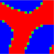
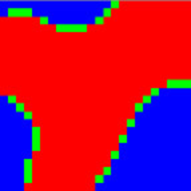
(a)	(b)
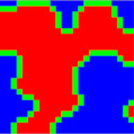
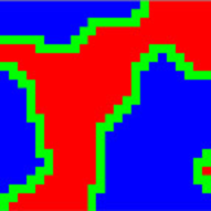
(c)	(d)

Figure 1: For $T=1/4$, detail of the border types: C (a), 0 (b), I (c) and II (d). Green squares represent vacancies.

In this paper we have chosen to determine the frontier between clusters via threshold values for the number of neighbors of different types, leading us to define borders of type C and 0, which have not been reported previously. We have opted for the term C because they form at the corners between different clusters, see Fig.1 (a). Departing from the C-type, and before reaching the complete configuration of a type-I site, we have found an intermediate border state defined by us as the 0-type, see Fig.1 (b). For type I and II we have conserved the nomenclature of [11]. As it is also explained in [11], these types of borders also appear for other combinations of parameters $T$ and $D$, so we have used $T=1/4$ as an illustration.

3.2 Avalanche processes

At this point, we proceed to increase the economic bias $H$ gradually by a fixed amount $\Delta H\gtrsim T/2$ every 50 time-steps. This value is approximately half of the one needed to start any avalanche process for a given neighborhood configuration. In the economic interpretation, the system offers less and less financial perspectives to blue agents, whose economic level and prospects are given by $\mu_{b}=D+H$. Meanwhile, red agents become more and more economically favored, $\mu_{r}=D-H$, thus enlarging the economic gap. Both expressions account for the dissatisfaction of an agent due to their economic conditions and their perspectives. Moreover, if we define the happiness associated to being in a specific neighborhood as $\lambda=T(N_{s}+N_{d})-N_{d}$, the satisfaction condition, Eq. (2), can be expressed now as

$$\mu_{r,b}\leq\lambda.$$ (8)

The interpretation of Eq. (8) is straightforward: when the satisfaction of being into a neighborhood, $\lambda$ compensates the unhapiness arising from the economic situation, $\mu_{r,b}$, the agent remains in the system. As we keep increasing $H$, the economic bias between $\mu_{r}$ and $\mu_{b}$ opens up. The system becomes less attractive towards blue agents, which increase $\mu_{b}$, and some of them are forced to leave when Eq. (8) ceases to hold. Therefore, there appear some new vacancies in the lattice. At the same time, the effect is opposite for red agents: $\mu_{r}$ decreases and the lattice is more satisfactory for them, because they are getting more and more economic advantages. Thus, red agents come from outside and occupy the vacancies previously created. Now, some of the blue agents close to these occupied locations cease to verify Eq. (8) because $\lambda$ has decreased for them due to the arrival of red agents. Thus, they may be transferred out of the system on subsequent time-steps. This gives rise to further new vacancies that are filled again with red agents and the process goes on in a self-sustained way. This is what we called a blue avalanche, because it originates with blue agents leaving the lattice.

Yet, there is another way to generate an avalanche. We depart from an equilibrium situation with some vacancies, which requires a mid-ranged economic environment, check Fig. 1 (b), (c) and (d). Before $H$ is strong enough to force blue agents out, red agents may be able to fill these vacancies up. Blue agents next to these locations may cease to verify Eq. (8), as in the previous situation, and are forced out of the system. These new vacancies are occupied by red agents from outside, making further blue agents leave. The process goes on, giving rise to what we will call a red avalanche.

The value of $H$ remains constant while these avalanches take place. After the avalanches are finished, if there are still some blue agents in the system the value of $H$ is increased further until a new avalanche takes place.

The similarity with a gentrification process is clear: one of the types of ageents find economical advantages by moving into this city zone, while the other is suffering the lack of financial opportunities and is forced out of the system, leaving vacancies on the borders between the two clusters. Meanwhile, red agents with better economic perspectives enter the system and occupy these vacancies. The process becomes self-sustained because other agents from the less favoured group are forced to leave the system due to their proximity to members of the other class. Of course, not all processes in the system give rise to an avalanche.

Avalanches will be characterized by their size $s$, defined as the total number of blue agents that have left the lattice as a consequence of the departure of the first one. We have obtained the avalanche size histograms, and fitted them to a probability density function (PDF) of the form

$$p(s)=Cx^{\alpha}\exp(-x/x_{0}),$$ (9)

where $C$ is the normalization constant, $\alpha$ accounts for the scaling exponent for the avalanches and $x_{0}$ acts as a maximal cutoff value. For reasons of numerical stability we focus on the complementary cumulative distribution function (CCDF) [18], which is fitted by the expression $C^{*}x^{\alpha+1}\exp-(x/x_{0})$. Data from 100 complete extinctions of the blue agents in the system have been measured for each $D$ value. For more numerical details, see A.

The next sections are devoted to the analysis of avalanche distributions for three values of $T$: low ($T=1/4$), medium ($T=1/2$) and high ($T=3/4$). For each value of $T$ we have characterized the behavior of the system for a wide range of fixed values of $D$, ranging from the situation where no vacancies are present to the extinction point in which, due to the high hostility of the medium all agents leave. We will vary $H$ in order to observe the avalanche processes for each $D$ value considered.

Let us introduce a convenient notation to describe neighborhoods, using s and d to denote similar and different neighbors, respectively, e.g. $3s+2d$ means that a certain agent has 3 similar and 2 dissimilar neighbors.

3.3 Avalanche distributions for $T=1/4$

We begin our study in a city with a high economic interest, $D=-2.125$ and low tolerance value $T=1/4$.

Under these circumstances the system exhibits a stationary state with big clusters of red and blue agents and no vacancies, due to the low value of $D$. Now, we increase $H$ gradually, $\mu_{b}$ becomes higher, and some blue agents may abandon the lattice. In fact, these blues agents are the ones which do not verify Eq. 8, and have $4s+4d$ neighbors. It must be noted that knowing the value of $T$ and the number of different and similar neighbors, $\lambda$ is fixed. Meanwhile, the situation for red agents keeps improving: $\mu_{r}$ becomes lower, so the vacancies created by the blue agents are filled by red agents coming from outside. This is what we defined previously as a blue avalanche (Sec. 3.2).

The system is so interesting economically for blue agents that they will adopt different strategies in order to remain, such as the formation of special cluster configurations: triangles and rectangles in contact with the system border. Thus, up to three avalanche processes can be needed to deplete the system of blue agents, as can be seen in Fig. 2 (a), where $D=-2.125$. To clarify the order in which each avalanche occurs and its kind (blue or red), we use the notation $\lambda_{n,k}$, where $n$ denotes the order and $k$ takes value $r$ for red and $b$ for blue ones. The fitted values for $\alpha$ and $x_{0}$ in all these cases are shown in Table 1.

For $D=-2.125$ and increasing $H$ gradually, we find that the first three avalanches start at treshold values $\lambda_{1,b}=-2.0$, $\lambda_{2,b}=-1.75$ and $\lambda_{3,b}=-1.0$. Extending our notation, we may say that each avalanche set has a dominant process, which is characterized by the typical neighborhood of the expelled blue agents and their $\lambda$ value. The values previously calcultaed correspond with certain neighborhood types: $4s+4d$, $2s+3d$ and $5s+3d$, respectively. Of course, no avalanche consists of a single type of process in practice. We must note that when blue agents with a higher $\lambda$ start their expulsion (such as $2s+3d$) those with an inferior treshold (for example $4s+4d$) can be still be in process of leaving. Thus, it is possible for various processes to take place simultaneously in the same avalanche. This is the situation for the first and second avalanche sets, $\lambda_{1,b}$ and $\lambda_{2,b}$ in Fig. 2 (a). The process $4s+4d$ dominates both avalanches so their curves are close to each other. As the avalanche for $\lambda_{3,b}$ is the last one for this $D$ value, it has a smaller size due the small number of blue agents remaining on the lattice.

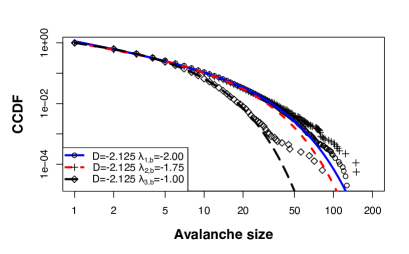
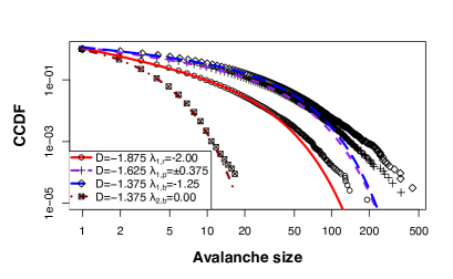
(a)	(b)

Figure 2: CCDF of the avalanche distribution sizes for $T=1/4$. For each curve the $D$ value is specified. Treshold values are given as $\lambda_{n,k}$ where $n$ is the avalanche set index and $k$ its kind: $r$ for reds, $b$ for blues and $p$ for purple ones. For purple avalanches upper and lower tresholds are expressed as $D\pm\lambda_{1,p}$. The fitted power-law cutoff functions are depicted with lines.

The social meaning is clear: the less favoured agents will try to stand on an economic advantageous environment despite their economic gap with the other group. To achieve this goal diverse neighborhood structures will be created (ghettos). This is the case scenario for neighborhoods as Harlem or Clinton Hills [19].

Now, let us focus our attention on higher values of $D$: $-1.875$, $-1.625$ and $-1.375$, as shown in Fig. 2 (b). Although the environment is still economically advantageous, the economic conditions are not as good as before. Some vacancies appear in the lattice and the system presents a C type of border (Fig. 1 (a)). As we explained before, different kinds of avalanches are still possible. The first one takes place for $D=-1.875$. Red agents coming from outside fill the existing vacancies on the system when $\mu_{r}\lesssim-2.0$. That points at a $4s+4d$ red avalanche with $\lambda_{1,r}=-2.00$ (Sec. 3.2). The next one, $D=-1.625$, is what we may call a purple avalanche: a simultaneous red avalanche with $\lambda_{1,r}=-2.00$ as in the former case, and a blue avalanche, $4s+3d$ with $\lambda_{1,b}=-1.25$, due to the overcoming of both tresholds at the same time ($D\pm H$). We must note that the $4s+3d$ is the vecindary associated with a 0-type border (Fig. 1(b)). So, while the red agents coming from outside are filling the vacancies with $4s+4d$ which correspond to a C-type border, blue agents with $4s+3d$ are leaving the system creating a 0-type border. Finally, we have blue avalanches for the first and second avalanche sets with $D=-1.375$, being their associated neighborhoods $4s+3d$ and $3s+1d$, respectively. The behavior of blue avalanches is similar to the ones explained for $D=-2.125$. Interestingly, red avalanches are more frequent than blue ones, although they present smaller sizes, as we can readily see in Fig. 2 (b) and Table 1. Red avalanches interfere among them, thus reducing the maximum cut-off, $x_{0}$.

The last value that we analyze for $T=1/4$ is $D=0.875$. The behaviour of the blue avalanche suffers an important change because the condition for a predominant vacancy state is verified, $D/T>3$ [11]. Combining eq. (2), with $H=0$, and Eq. (3) the condition for an agent to remain on the system can be written as $N_{d}\leq(N_{s}-D/T)/(1/T-1)$. As $T$ is lower than unity, the denominator stays positive, so the numerator of the former equation dictates the agent behaviour. Any agent must fulfill the condition $N_{s}\geq D/T$ to remain on the lattice, even if no different agent is in the vecindary. As the system initial configuration is random and both kinds of agents and vacancies are equally likely, the probability for an agent to have more than three similar neighbors is small. Therefore, when $D/T>3$ the system becomes very hostile, agents leave massively, and only a small number of them remain inside clusters, shortening $x_{0}$ (Fig 3 a). The border between clusters is not relevant anymore: red clusters grow with a vecindary as $(3s+0d)$ and blue ones become smaller when agents have a neighborhood $(4s+0d)$ (Fig 3 (b) and (c)).

Socially, the situation for blue agents might be compared to the Chicago suburbs where the population could increase their personal ties via a community network [11]. These ties may prevent a massive exodus despite the lack of attractiveness of the environment. However, in our model, the evolution of the system departs from this situation and develops in two opposite directions: blue agents are removed from the system due to the hostile environment and the lack of economic prospects, in contrast to red agents, which increase their population finding good opportunities. This could be understood as the unrelated behavior of two communities. One of them chooses to cooperate and the ensuing growth overcomes economical hardships. The other one is unable to strengthen their links and leaves the city.

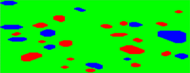
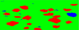
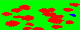
(a)	(b)	(c)

Figure 3: From left to right: snapshot of the system evolution for T=1/4 and D=0.875. Equilibrium (a), 6 MC steps (b) and 13 MC steps (c). Green squares represent vacancies.

Finally, we show the values of the fitted parameters in Table 1, being $x_{c}$ the choosen size for the fitting (A). We can find $\alpha$ values in the range $[-1.78,-0.98]$ previously reported in references [20, 21, 22, 23], concerning self-organized criticality in different systems.

$B$	$A$	$D$	$\alpha$	$x_{0}$	$x_{c}$	$C$
N	b	$-2.125$	$-1.781\pm 0.002$	$16.2\pm 0.3$	$40$	$1.20\pm 0.03$
C	r	$-1.875$	$-1.77\pm 0.02$	$15.0\pm 0.3$	$30$	$1.15\pm 0.02$
C	p	$-1.625$	$-1.50\pm 0.01$	$24.7\pm 0.6$	$50$	$1.20\pm 0.03$
C	b	$-1.375$	$-1.38\pm 0.02$	$23.7\pm 0.5$	$50$	$1.21\pm 0.03$
0	r	$-1.125$	$-1.37\pm 0.03$	$3.30\pm 0.04$	$20$	$1.42\pm 0.04$
0	p	$-0.875$	$-1.716\pm 0.008$	$42.8\pm 0.9$	$50$	$1.13\pm 0.02$
0	b	$-0.625$	$-1.618\pm 0.004$	$140\pm 1$	$240$	$1.23\pm 0.02$
I	r	$-0.375$	$-1.35\pm 0.02$	$18.0\pm 0.3$	$40$	$1.14\pm 0.02$
I	p	$-0.125$	$-1.463\pm 0.004$	$79.2\pm 0.6$	$150$	$1.15\pm 0.01$
I	b	$0.125$	$-1.495\pm 0.005$	$181\pm 4$	$200$	$1.26\pm 0.02$
II	r	$0.375$	$-1.136\pm 0.007$	$20.9\pm 0.2$	$50$	$1.12\pm 0.01$
II	p	$0.625$	$-1.41\pm 0.03$	$69.9\pm 0.4$	$150$	$1.081\pm 0.008$
V	rb	$0.875$	$-1.33\pm 0.02$	$9.6\pm 0.3$	$20$	$1.15\pm 0.02$

Table 1: Avalanche distribution parameters $(T=1/4)$ for $D$ values from (Section 3.3). $B$ is the type of border, with ’V’ meaning vacancy dominated regime. $A$ is the avalanche type, (’b’ is blue, ’p’ is purple and ’r’ is red), $\alpha$ is the power law exponent, $x_{0}$ accounts for cutoff value and $x_{c}$ is the chosen size for the fitting (see A).

3.4 Avalanche distributions for $T=1/2$ and $T=3/4$

Most of the processes that arise for these values of $T$ are avalanches with similar parameter values and behaviours to those explained in the previous section (Sec. 3.3).

Nevertheless, as this $T$ fixed value is larger than before, the dissatisfaction index disminishes and Eq. 8 is verified for higher values of $D$. Thus, despite being in a less economically interesting system, agents populate the lattice. As a consequence the range of values of $D$ for which the system is vacancy dominated increases.

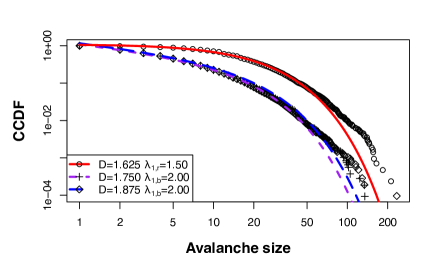
Figure 4: CCDF of the avalanche distributions for $T=1/2$ in the predominant vacancy state, represented by symbols. The fitted power-law cutoff functions are depicted with lines.

The two last avalanches for $T=1/2$, $D=1.750$ (short dash) and $D=1.875$ (long dash) are in the predominant vacancy state (Fig. 4). They are also really close to each other, suggesting that the same mechanism takes place and it is related to $4s+0d$ neighborhoods with $\lambda_{1,b}=2.00$. This process implies that the blue agents will be expelled when they are surrounded by vacancies.

The system evolution for $D=1.750$ is apparently similar to the one in Fig. 3. Nonetheless, the environment has become so hard that red agents are not able to expand as the blue agents progressively leave the city, converting a purple avalanche into a blue one. From a social perspective it can be explained as people leaving the city looking for a better financial situation somewhere else, abandoning the neighborhood into obliteration.

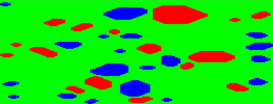
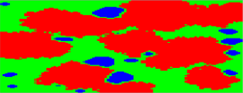
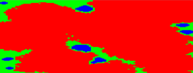
(a)	(b)	(c)

Figure 5: From left to right: snapshot of the system evolution with $T=1/2$ and $D=1.625$. Equilibrium (a), 30 MC steps (b) and 50 MC steps (c).

One of the most interesting processes in our work takes place for $D=1.625$ (continuous), and is also found in the predominant vacancy state (Fig. 4). It is convenient to depict its evolution in Fig. 5. As it is shown, the first procedure that takes place is the red cluster expansion (Fig. 5 b)) for the neighborhood $3s+0d$ which takes place when $\mu_{r}\lesssim 1.5$. This mechanism proceeds until a blue cluster is found. As the red cluster grows, the population increases. When both kinds of agents are close, the $4s+1d$ red avalanche removes all blue agents. For this $D$ value, $\alpha=-0.97\pm 0.01$, $x_{0}=17.4\pm 0.3$.

This two stage process may be interpreted as the expansion of some kind of neighborhoods that improve their economical perspectives and are able to increase their size, wrapping around other devaluated zones. After that, a gentrification process starts. This process is reminiscent of the transformation of small towns or villages close to growing commuting zones [24].

Finally, for $T=3/4$, multiple $D$ values are found in the vacancy dominated regime, but all the situations are related to those previously explained. Type of borders 0, I and II are found to be in this situation.

When the system is in the predominant vacancy state, there are only two processes that guarantee the complete removal of blue agents. The first one is associated with $3s+0d$ neighborhoods and consist of the red cluster expansion, which changes the environment. After that, other complementary processes take place (as in Fig. 5). The other one is related to $4s+0d$ neighborhoods, which implies the total expulsion of blue agents surrounded by vacancies (Fig. 3). As a consequence, fitted parameters are close to the ones previously calculated for other values of $T$ in the same situations.

4 Conclusion

The generalization of the open city model provides a new framework for the study and understanding of a broad class of urban processes, i.e. gentrification. Besides analyzing its results from a social and economical perspective, the model is also linked with the physics of the BEG model under the influence of an external magnetic field.

As agents can leave or enter the city, not only tolerance but two economic terms are taken into consideration: $D$ is associated with the mean economic city level, and $H$ stands for the economic attractivity gap between both types of agents. The dynamical rules are the following: once the system has evolved into an equilibrium state, fixing $T$ and $D$, $H$ progressively increases. In the economical sense, there are worse financial perspectives for blue agents, meanwhile, red agents are finding better opportunities, and an economic gap is created. Some blue agents, generally the ones that are closer to the red agents, begin to leave the city. These new vacancies are occupied by red agents coming from outside, so the process goes on in a self-sustained way, and resembles gentrification.

A power law with exponential cutoff expression has been used to describe the avalanche size histograms. While the cutoff length depends on the system size, the power law exponents are in the range $[-1.781,-0.97]$, values that can be found in the literature for diverse avalanche processes.

In our modified Schelling model gentrification processes could also help understand the formation of ghettos, as special configuration of the less favoured class in order to remain in the cities. Moreover, our results highlight the importance of tolerance and ties for people to be satisfied despite harsh conditions. On one hand, collaboration inside of a neighborhood implies an improving in economic and trading exchanges, making growth possible. On the other hand the lack of economic stimulus in a disfavorable environment results in the neighborhood progressive degradation.

Further analysis should focus on variants in which agents consider different economic zones. For example, the city centre is usually more valuable than the outskirts. Furthermore, it could be also interesting to study the distribution of the inter-event times between the avalanches shown in this work. Finally, we consider that the presented framework could also allow us to study a recent urban phenomena: the relocation of workers with telecommuting possibilities outside the cities due to COVID19 pandemic.

Appendix A Fitting the avalanche histograms

Some numerical difficulties associated with direct estimation of $\alpha$ and $x_{0}$ from the probability density function (PDF) of the histograms are known to arise [18]. In order to address them, we have resorted to the use of the complementary cumulative distribution function (CCDF). Our analytical form is given by Eq. (10).

$$\begin{split}P(s)&=Pr(X>s)\\ &=\int_{s}^{\infty}Cx^{\alpha}\exp(-x/x_{0})dx\\ &=F(\alpha,x_{0})+G(\alpha,x_{0})s^{\alpha+1}\exp-(s/x_{0})\\ &\cdot\left[1+\frac{1}{2+\alpha}\frac{s}{x_{0}}+...\right].\end{split}$$ (10)

The terms inside the brackets are an expansion of $\mathbf{M}(1,2+\alpha,s/x_{0})$, where $\mathbf{M}$ is the confluent hypergeometric function. Once $\alpha$ and $x_{0}$ have been estimated, both $F(\alpha,x_{0})$ and $G(\alpha,x_{0})$ take fixed values. In fact, $F(\alpha,x_{0})$ does not introduce significative changes in the fit, and it can be neglected. Under these circumstances, and retaining only the leading term of the series, we have

$$P(s)\approx G(\alpha,x_{0})x^{\alpha+1}\exp(-x/x_{0}).$$ (11)

Consequently, we can infer the exponent $\alpha$ and the length $x_{0}$ of an avalanche from the CCDF of the avalanche histogram.

The experimental CCDF data series in our avalanches have been calculated from 100 complete extinctions of the blue agents. After that, data are plotted with a constant bin size by means of the poweRlaw R package [25]. Then an expression of the type $C^{*}x^{\alpha+1}\exp-(x/x_{0})$, where $C^{*}\approx G(\alpha,x_{0})$ is fitted by the nonlinear least square method from the stats subroutines [26]. Although the curves have been depicted for a wide avalanche size range, they have been fitted inside the interval $[1,x_{c})$, being $x_{c}$ a choosen value to uphold precision. Deviations between data and fit can appear for $s\gg x_{0}$, due to the series expansion approximation and the own nature of the tail distribution, but they are not relevant. As a practical rule, if $x_{0}<60$ then $x_{c}\leq 2x_{0}$ (see Table 1). Choosing $x_{c}$ in this way, the precision of the fit improves for a wide range of avalanche size values.

References

- [1] N. Smith, New globalism, new urbanism: Gentrification as global urban strategy, Antipode (34) (2009) 427.
- [2] T. Schelling, Dynamic models of segregation, Journal of Mathematical Sociology (1) (1971) 143–186.
- [3] L. Gauvin, J. Vannimenus, J.-P. Nadal, Phase diagram of a Schelling segregation model, The European Physical Journal B 70 (2) (2009) 293–304. doi:10.1140/epjb/e2009-00234-0.
- [4] L. Dall’Asta, C. Castellano, M. Marsili, Statistical physics of the Schelling model of segregation, Journal of Statistical Mechanics: Theory and Experiment 2008 (07) (2008) L07002. doi:10.1088/1742-5468/2008/07/L07002.
- [5] E. V. Albano, Interfacial roughening, segregation and dynamic behaviour in a generalized Schelling model, Journal of Statistical Mechanics-Theory and Experiment (2012) P03013doi:10.1088/1742-5468/2012/03/P03013.
- [6] N. Houy, Forecasts in Schelling’s segregation modelArXiv: 1911.08191.
- [7] P. Jensen, T. Matreux, J. Cambe, H. Larralde, E. Bertin, Giant catalytic effect of altruists in Schelling’s segregation model, Physical Review Letters 120 (20) (2018) 208301, arXiv: 1803.10505.
- [8] S. Grauwin, E. Bertin, R. Lemoy, P. Jensen, Competition between collective and individual dynamics, Proceedings of the National Academy of Sciences 106 (49) (2009) 20622–20626. doi:10.1073/pnas.0906263106.
- [9] M. Fossett, D. R. Dietrich, Effects of city size, shape, and form, and neighborhood size and shape in agent-based models of residential segregation: are Schelling-style preference effects robust?, Environment and Planning B-Planning & Design 36 (1) (2009) 149–169, wOS:000263711600010. doi:10.1068/b33042.
- [10] E. J. Laurie, N. K. Jaggi, Role of ‘vision’ in neighbourhood racial segregation: a variant of the Schelling segregation model, Urban Studies (2003) 2687–2704.
- [11] L. Gauvin, J.-P. Nadal, J. Vannimenus, Schelling segregation in an open city: A kinetically constrained Blume-Emery-Griffiths spin-1 system, Physical Review E 81 (6) (2010) 066120. doi:10.1103/PhysRevE.81.066120.
- [12] G. Barmpalias, R. Elwes, A. Lewis-Pye, Unperturbed Schelling Segregation in Two or Three Dimensions, Journal of Statistical Physics 164 (6) (2016) 1460–1487. doi:10.1007/s10955-016-1589-6.
- [13] F. Gargiulo, Y. Gandica, T. Carletti, Emergent Dense Suburbs in a Schelling Metapopulation Model: A Simulation Approach, Advances in Complex Systems 20 (1) (2017) 1750001. doi:10.1142/S0219525917500011.
- [14] P. Bak, How Nature Works: The Science of Self-organized Criticality, Oxford University Press, 1997.
- [15] M. Bartolozzi, D. B. Leinweber, A. W. Thomas, Scale-free avalanche dynamics in the stock market, Physica A: Statistical Mechanics and its Applications 370 (1) (2006) 132–139.
- [16] M. Blume, V. J. Emery, R. B. Griffiths, Ising Model for the Transition and Phase Separation in and Mixtures, Physical Review A 4 (3) (1971) 1071–1077.
- [17] B. Simon, The statistical mechanics of lattice gases, Princeton University Press, 1993.
- [18] A. Clauset, C. R. Shalizi, M. E. J. Newman, Power-Law Distributions in Empirical Data, SIAM Review 51 (4) (2009) 661–703. doi:10.1137/070710111.
- [19] L. Freeman, There goes the ’hood: view of gentrification from the ground up, Temple University Press, 2006.
- [20] P. Bak, C. Tang, K. Wiesenfeld, Self-organized criticality: An explanation of the 1/f noise, Physical Review Letters 59 (4) (1987) 381–384. doi:10.1103/PhysRevLett.59.381.
- [21] M. A. Muñoz, R. Dickman, A. Vespignani, S. Zapperi, Avalanche and spreading exponents in systems with absorbing states, Physical Review E 59 (5) (1999) 6175–6179. doi:10.1103/PhysRevE.59.6175.
- [22] R. Batac, A. Paguirigan Jr, A. Tarun, A. Longjas, Sandpile-based model for capturing magnitude distributions and spatiotemporal clustering and separation in regional earthquakes, Nonlinear Processes in Geophysics 24 (2017) 179–187. doi:10.5194/npg-24-179-2017.
- [23] N. Zachariou, P. Expert, M. Takayasu, K. Christensen, Generalised Sandpile Dynamics on Artificial and Real-World Directed Networks, PLOS ONE 10 (11) (2015) e0142685. doi:10.1371/journal.pone.0142685.
- [24] C. P. Swanson, Man’s Role in Changing the Face of the Earth. William L. Thomas, Jr., The Quarterly Review of Biology 32 (3) (1957) 319–320. doi:10.1086/401971.
- [25] C. S. Gillespie, Fitting Heavy Tailed Distributions: The poweRlaw Package, Journal of Statistical Software 64 (1) (2015) 1–16. doi:10.18637/jss.v064.i02.
- [26] R. C. Team, R: A language and environment for statistical computing (2020).