Interpretable Fault Detection using Projections of Mutual Information Matrix

Abstract

This paper presents a novel mutual information (MI) matrix based method for fault detection. Given a $m$-dimensional fault process, the MI matrix is a $m\times m$ matrix in which the $(i,j)$-th entry measures the MI values between the $i$-th dimension and the $j$-th dimension variables. We introduce the recently proposed matrix-based Rényi’s $\alpha$-entropy functional to estimate MI values in each entry of the MI matrix. The new estimator avoids density estimation and it operates on the eigenspectrum of a (normalized) symmetric positive definite (SPD) matrix, which makes it well suited for industrial process. We combine different orders of statistics of the transformed components (TCs) extracted from the MI matrix to constitute the detection index, and derive a simple similarity index to monitor the changes of characteristics of the underlying process in consecutive windows. We term the overall methodology “projections of mutual information matrix” (PMIM). Experiments on both synthetic data and the benchmark Tennessee Eastman process demonstrate the interpretability of PMIM in identifying the root variables that cause the faults, and its superiority in detecting the occurrence of faults in terms of the improved fault detection rate (FDR) and the lowest false alarm rate (FAR). The advantages of PMIM is also less sensitive to hyper-parameters. The advantages of PMIM is also less sensitive to hyper-parameters. Code of PMIM is available at https://github.com/SJYuCNEL/Fault_detection_PMIM.

1 Introduction

With the growing demand for security equipments and high-quality products, process monitoring has received tremendous attention in both academia and industry in the past decades. Fault detection, defined as the identification of abnormal operating conditions in real time, is an active topic in process monitoring. Data driven approaches have been the main stream for fault detection and control in recent years because they don’t require neither a model not a priori information [1, 2]. The multivariate statistical process monitoring (MSPM) is a well-known data-driven approach, and has been widely used in complex industrial environments [3, 4, 5].

Traditional MSPM methods, e.g., principal component analysis (PCA) [6], partial least squares (PLS) [7] and independent component analysis (ICA) [8], take advantage of the Hotteling $T^{2}$ statistic in principal component subspace or the squared prediction error (SPE) statistic in residual subspace to monitor the sample stream [9, 10]. Although this kind of methods perform satisfactorily in the case of highly correlated multi-modal variables, they always neglect the temporal correlation between consecutive samples. Consequently, they cause a large Type-II error (i.e., fails to reject a false null-hypothesis).

To circumvent this limitation, the dynamic PCA (DPCA) [11, 12], the modified ICA (MICA) [13, 14, 15] and various other recursive MSPM methods (e.g., [16, 17, 18, 19]) have been proposed thereafter. These methods usually add time-lagged variables in a sliding window to form a data matrix that captures the (local) dynamic characteristics of the underlying process. Compared with the traditional PCA or ICA, window-based methods distinguish better sample measurement from noise, thus offering a reliable avenue to address challenges associated with continuous processes [20, 21].

To further improve the performance of the above window-based methods, efficient extraction of high-order statistics of process variables is crutial [22, 23, 24, 25, 21, 26]. Notable examples include statistics pattern analysis (SPA) [20, 23], recursive transformed component statistical analysis (RTCSA) [24] and recursive dynamic transformed component statistical analysis (RDTCSA) [25]. Different from traditional PCA and DPCA that implicitly assume that the latent variables follow a multivariate Gaussian distribution, SPA integrates the skewness, the kurtosis, and various other high-order statistics of the process measurement in sliding windows to deal with non-Gaussian data, demonstrating superior performance over PCA and DPCA. However, SPA performs poorly in case of incipient faults [24]. To address this limitation, RTCSA and RDTCSA avoid dividing the projected space into principal component subspace and residual subspace. Instead, both methodologies take advantage of the full space to extract orthogonal transformed components (TCs), and evaluate a test statistic by incorporating the mean, the variance, the skewness, and the kurtosis of TCs. One should note that, the third- and forth-order information is usually beneficial to detect incipient faults [22, 20, 23, 24, 25, 21]. Although RTCSA and RDTCSA enjoy solid mathematical foundation, the TCs from a covariance matrix only capture linear relationships among different dimensions of measurement. Therefore, a reliable way to extract nonlinear statistics among different dimensions of measurements becomes a pivotal problem in fault detection [27, 28, 29].

The application of information theory on fault detection is an emerging and promising topic [30, 31]. Although there are a few early efforts that attempt to shed light on fault detection with information-theoretic concepts, they simply employ (an approximation to) the MI to select a subset of the most informative variables to circumvent the curse of dimensionality (e.g., [32, 33, 34, 35, 36, 37]). To the best of our knowledge, there are only two exceptions that illuminate the potential of using information-theoretic concepts for fault detection, beyond the role of variable selection. Unfortunately, no specific statistical analysis is presented [36, 37]. Therefore, the design from first principles of a fault detection method using information theory remains an open problem. The detailed contribution of this work is multi-fold:

• Novel methodology: We construct a MI matrix to monitor the (possibly nonlinear) dynamics and the non-stationarity of the fault process. A novel fault detection method, i.e., projections of mutual information matrix (PMIM), is also developed thereafter.

• Novel estimator: Unlike previous information-theoretic fault detection methods which usually use the classical Shannon entropy functional that relies heavily on the precise estimation of underlying data distributions, we suggest using the recently proposed matrix-based Rényi’s $\alpha$-entropy functional to estimate MI values. The new estimator avoids estimation of the underlying probability density function (PDF), and employs the eigenspectrum of a (normalized) symmetric positive definite (SPD) matrix. This intriguing property makes the novel estimator easily applicable to real-world complex industrial process which usually contains continuous, discrete and even mixed variables.

• Detection accuracy: Experiments on both synthetic data and the benchmark Tennessee Eastman process (TEP) indicate that PMIM achieves comparable or slightly higher detection rates than state-of-the-art fault detection methods. Moreover, PMIM enjoys significantly lower false detection rate.

• Implementation details and reproducibility: We elaborate the implementation details of fault detection using PMIM. We also illustrate the detectability of PMIM using the eigenspectrum of the MI matrix. For reproducible results, we provide key functions (in MATLAB $2019$a) concerning PMIM in the Appendix A. We also release a full demo of PMIM at https://github.com/SJYuCNEL/Fault_detection_PMIM.

• Interpretability: Fault detection using PMIM can provide insights on the the exact root variables that lead to the occurrence of fault. In this sense, the result of fault detection using PMIM is interpretable, i.e., the practitioners know which variable or specific sensor data causes the fault.

The remainder of this paper is organized as follows. We first introduce the definition of MI matrix and present its estimation with the matrix-based Rényi’s entropy functional in Section 2. We then describe our proposed fault detection using PMIM in Section 3, and elaborate its implementation details in Section 4. Experiments on both synthetic and TEP benchmark are performed in Section 5. We finally conclude this work and discuss future directions in Section 6.

Notations: Throughout this paper, scalars are denoted by lowercase letters (e.g., $x$), vectors appear as lowercase boldface letters (e.g., $\mathbf{x}$), and matrices are indicated by uppercase letters (e.g., $X$). The $(i,j)$-th element of $X$ is represented by $X_{ij}$. If $X$ is a square matrix, then $X^{-1}$ denotes its inverse. $I$ stands for the identity matrix with compatible dimensions. The $i$-th row of a matrix $X$ is declared by the row vector $\mathbf{x}^{i}$, while the $j$-th column is indicated with the column vector $\mathbf{x}_{j}$. Moreover, superscript indicates time (or sample) index, subscript indicates variable index. For $\mathbf{x}\in\mathbb{R}^{n}$, the $\ell_{p}$-norm of $\mathbf{x}$ is defined as $\|\mathbf{x}\|_{p}\triangleq(\sum\limits_{i=1}^{n}|x_{i}|^{p})^{\frac{1}{p}}$.

2 The MI Matrix: Definition and Estimation

2.1 The Definition of MI matrix

MI quantifies the nonlinear dependence between two random variables [39, 40]. Therefore, given a multivariate time series (here refers to fault process), an MI matrix (in a stationary environment) can be constructed by evaluating MI values between each pair of variables. Intuitively, the MI matrix can be viewed as a nonlinear extension of the classical covariance matrix. Specifically, the formal definition of MI matrix is given as follows.

Definition 1. Given a $m$-dimensional (stationary) process $\wp$, let us denote $\mathbf{x}_{i}$ ($i=1,2,\cdots,m$) the $i$-th dimensional of the process measurement, then the MI matrix over $\wp$ is defined as:

$$M=\begin{bmatrix}I(\mathbf{x}_{1};\mathbf{x}_{1})&I(\mathbf{x}_{1};\mathbf{x}_{2})&\cdots&I(\mathbf{x}_{1};\mathbf{x}_{m})\\ I(\mathbf{x}_{2};\mathbf{x}_{1})&I(\mathbf{x}_{2};\mathbf{x}_{2})&\cdots&I(\mathbf{x}_{2};\mathbf{x}_{m})\\ \vdots&\vdots&\ddots&\vdots\\ I(\mathbf{x}_{m};\mathbf{x}_{1})&I(\mathbf{x}_{m};\mathbf{x}_{2})&\cdots&I(\mathbf{x}_{m};\mathbf{x}_{m})\\ \end{bmatrix}\in\mathbb{R}^{m\times m},$$ (1)

where $I(\mathbf{x}_{i};\mathbf{x}_{j})$ denotes MI between variables $\mathbf{x}_{i}$ and $\mathbf{x}_{j}$.

According to Shannon information theory [38], $I(\mathbf{x}_{i};\mathbf{x}_{j})$ is defined over the joint probability distribution of $\mathbf{x}_{i}$ and $\mathbf{x}_{j}$ (i.e., $p(\mathbf{x}_{i},\mathbf{x}_{j})$) and their respectively marginal distributions (i.e., $p(\mathbf{x}_{i})$ and $p(\mathbf{x}_{j})$). Specifically,

$$\begin{split}I(\mathbf{x}_{i};\mathbf{x}_{j})&\!=\!\!\int\!\!\int\!\!p(\mathbf{x}_{i},\mathbf{x}_{j})\log\left(\frac{p(\mathbf{x}_{i},\mathbf{x}_{j})}{p(\mathbf{x}_{i})p(\mathbf{x}_{j})}\right)d\mathbf{x}_{i}d\mathbf{x}_{j}\\ &=-\int\!\!\left(\!\!\int\!\!p(\mathbf{x}_{i},\mathbf{x}_{j})d\mathbf{x}_{j}\!\!\right)\!\!\log p(\mathbf{x}_{i})d\mathbf{x}_{i}\!\!-\!\!\int\!\!\left(\!\!\int\!\!p(\mathbf{x}_{i},\mathbf{x}_{j})d\mathbf{x}_{i}\!\!\right)\!\!\log p(\mathbf{x}_{j})d\mathbf{x}_{j}\\ &~{}~{}~{}~{}+\int\int p(\mathbf{x}_{i},\mathbf{x}_{j})\log p(\mathbf{x}_{i},\mathbf{x}_{j})d\mathbf{x}_{i}d\mathbf{x}_{j}\\ &=-\int\!\!p(\mathbf{x}_{i})\log p(\mathbf{x}_{i})d\mathbf{x}_{i}\!-\!\!\int\!\!p(\mathbf{x}_{j})\log p(\mathbf{x}_{j})d\mathbf{x}_{j}\!+\!\!\int\!\!\int\!\!p(\mathbf{x}_{i},\mathbf{x}_{j})\log p(\mathbf{x}_{i},\mathbf{x}_{j})d\mathbf{x}_{i}d\mathbf{x}_{j}\\ &\!\!=\!\!H(\mathbf{x}_{i})\!+\!H(\mathbf{x}_{j})\!-\!H(\mathbf{x}_{i},\mathbf{x}_{j}),\end{split}$$ (2)

where $H(\cdot)$ denote the entropy and $H(\cdot,\cdot)$ denotes the joint entropy. In particular, $I(\mathbf{x}_{i};\mathbf{x}_{i})=H(\mathbf{x}_{i})$.

Theoretically, the MI matrix is symmetric and non-negative. Moreover, in the absence of any dependence in pairwise variables, the MI matrix reduces to a diagonal matrix with the entropy of each variable lies on the main diagonal. Interestingly, although the estimated MI matrix has been conjectured and also observed in our application to be positive semidefinite, this property is not always true theoretically [41].

2.2 Estimate MI matrix with matrix-based Rényi’s $\alpha$-order entropy

Entropy measures the uncertainty in a random variable using a single scalar quantity [42, 43]. For a random variable (or vector) $\mathbf{x}$, with probability density function (PDF) $p(\mathbf{x})$ in a finite set $\mathbf{s}$, a natural extension of the Shannon’s differential entropy is the Rényi’s $\alpha$-order entropy [44]:

$$H_{\alpha}(\mathbf{x})=\frac{1}{1-\alpha}\log\int_{\mathbf{s}}p^{\alpha}(\mathbf{x})d\mathbf{x}.$$ (3)

It is well-known that, when $\alpha\to 1$, Eq. (3) reduces to the basic Shannon’s differential entropy $H(\mathbf{x})=-\int_{\mathbf{s}}p(\mathbf{x})\log p(\mathbf{x})d\mathbf{x}$. In this perspective, Rényi’s entropy makes a one-parameter generalization to the basic Shannon definition by introducing a hyperparameter $\alpha$.

Information theory has been successfully applied to various machine learning, computer vision and signal processing tasks [42, 46]. Unfortunately, the accurate PDF estimation in Eq. (3) on continuous and complex data impedes its more widespread adoption in data driven science. This problem becomes more severe for process monitoring, since the obtained multivariate measurement may contain both discrete and continuous variables. Moreover, there is still no universal agreement on the definition of MI between discrete and continuous variables [47, 48], let alone its precise estimation. In this work, we use a novel estimator developed by Sánchez Giraldo et al. [49] to estimate the MI matrix. Specifically, according to [46, 49], it is feasible to evaluate a quantity that resembles quantum Rényi’s entropy [44] in terms of the normalized eigenspectrum of the Hermitian matrix of the projected data in reproducing kernel Hilbert space (RKHS), thus estimating the entropy directly from data without PDF estimation. For completeness, we provide below Sánchez Giraldo et al.’s definition on entropy and joint entropy.

Definition 2. Let $\kappa:\chi\times\chi\mapsto\mathbb{R}$ be a real valued positive definite kernel that is also infinitely divisible [50]. Given $\{\mathbf{x}_{i}\}_{i=1}^{n}\in\chi$, each $\mathbf{x}_{i}$ can be a real-valued scalar or vector, and the Gram matrix $K$ obtained from evaluating a positive definite kernel $\kappa$ on all pairs of exemplars, that is $K=\kappa(\mathbf{x}_{i},\mathbf{x}_{j})$, a matrix-based analogue to Rényi’s $\alpha$-entropy for a normalized positive definite matrix $A$ of size $n\times n$, such that $\operatorname{tr}(A)=1$, can be given by the following functional:

$$H_{\alpha}(A)=\frac{1}{1-\alpha}\log\left(\operatorname{tr}(A^{\alpha})\right)=\frac{1}{1-\alpha}\log_{2}\left(\sum_{i=1}^{n}\lambda_{i}(A)^{\alpha}\right),$$ (4)

where $A$ is the normalized version of $K$, i.e., $A=K/{\text{tr}(K)}$, and $\lambda_{i}(A)$ denotes the $i$-th eigenvalue of $A$.

Definition 3. Given $n$ pairs of samples $(\mathbf{x}_{i},\mathbf{y}_{i})_{i=1}^{n}$, each sample contains two different types of measurements $\mathbf{x}\in\chi$ and $\mathbf{y}\in\gamma$ obtained from the same realization, and the positive definite kernels $\kappa_{1}:\chi\times\chi\mapsto\mathbb{R}$ and $\kappa_{2}:\gamma\times\gamma\mapsto\mathbb{R}$ , a matrix-based analogue to Rényi’s $\alpha$-order joint-entropy can be defined as:

$$H_{\alpha}(A,B)=H_{\alpha}\left(\frac{A\circ B}{\operatorname{tr}(A\circ B)}\right),$$ (5)

where $A_{ij}=\kappa_{1}(\mathbf{x}_{i},\mathbf{x}_{j})$ , $B_{ij}=\kappa_{2}(\mathbf{y}_{i},\mathbf{y}_{j})$ and $A\circ B$ denotes the Hadamard product between the matrices $A$ and $B$.

Given Eqs. (4)-(5), the matrix-based Rényi’s $\alpha$-order MI $I_{\alpha}(A;B)$ in analogy of Shannon’s MI is given by:

$$I_{\alpha}(A;B)=H_{\alpha}(A)+H_{\alpha}(B)-H_{\alpha}(A,B).$$ (6)

Throughout this paper, we use the Gaussian kernel $\kappa(\mathbf{x}_{i},\mathbf{x}_{j})=\exp(-\frac{\|\mathbf{x}_{i}-\mathbf{x}_{j}\|^{2}}{2\sigma^{2}})$ to obtain the Gram matrices. Obviously, Eq. (6) avoids real-valued PDF estimation and has no additional requirement on data characteristics (e.g., continuous, discrete, or mixed), which makes it has great potential in our application.

3 The Fault Detection using PMIM

In this section, we present PMIM, a novel fault detection method by monitoring the statistics associated with the MI matrix. Given a discrete time process $\aleph=\{\mathbf{x}^{1},\mathbf{x}^{2},\cdots\}:\mathbf{x}^{i}\in\mathbb{R}^{1\times m}$, at each time instant $k$, we construct a local sample matrix $X^{k}\in\mathbb{R}^{w\times m}$ of the following form:

$$\begin{split}X^{k}&=\begin{bmatrix}\mathbf{x}^{k-w+1}\\ \mathbf{x}^{k-w+2}\\ \vdots\\ \mathbf{x}^{k}\end{bmatrix}=\begin{bmatrix}x^{k-w+1}_{1}&x^{k-w+1}_{2}&\cdots&x^{k-w+1}_{m}\\ x^{k-w+2}_{1}&x^{k-w+2}_{2}&\cdots&x^{k-w+2}_{m}\\ \vdots&\vdots&\ddots&\vdots\\ x^{k}_{1}&x^{k}_{2}&\cdots&x^{k}_{m}\end{bmatrix}\\ &\triangleq\left[\begin{array}[]{c;{2pt/2pt}c;{2pt/2pt}c;{2pt/2pt}c}\mathbf{x}_{1}&\mathbf{x}_2&\cdots&\mathbf{x}_{m}\end{array}\right]\in\mathbb{R}^{w\times m},\end{split}$$ (7)

where $\mathbf{x}_{j}$ ($1\leq j\leq m$) denotes the $j$-th dimensional variable that is characterized by $w$ realizations. Fig. 1 illustrates $\mathbf{x}^{i}$, $\mathbf{x}_{j}$ and $X$. Each variable is mean centered and normalized to $[0,1]$ to account for different value ranges [3, 4, 5, 6, 7]. Then the MI matrix $M$ at time instant $k$ is given by:

$$M=\begin{bmatrix}H(\mathbf{x}_{1})&I(\mathbf{x}_{1};\mathbf{x}_{2})&\cdots&I(\mathbf{x}_{1};\mathbf{x}_{m})\\ I(\mathbf{x}_{2};\mathbf{x}_{1})&H(\mathbf{x}_{2})&\cdots&I(\mathbf{x}_{2};\mathbf{x}_{m})\\ \vdots&\vdots&\ddots&\vdots\\ I(\mathbf{x}_{m};\mathbf{x}_{1})&I(\mathbf{x}_{m};\mathbf{x}_{2})&\cdots&H(\mathbf{x}_{m})\end{bmatrix}\in\mathbb{R}^{m\times m}\\ .$$ (8)

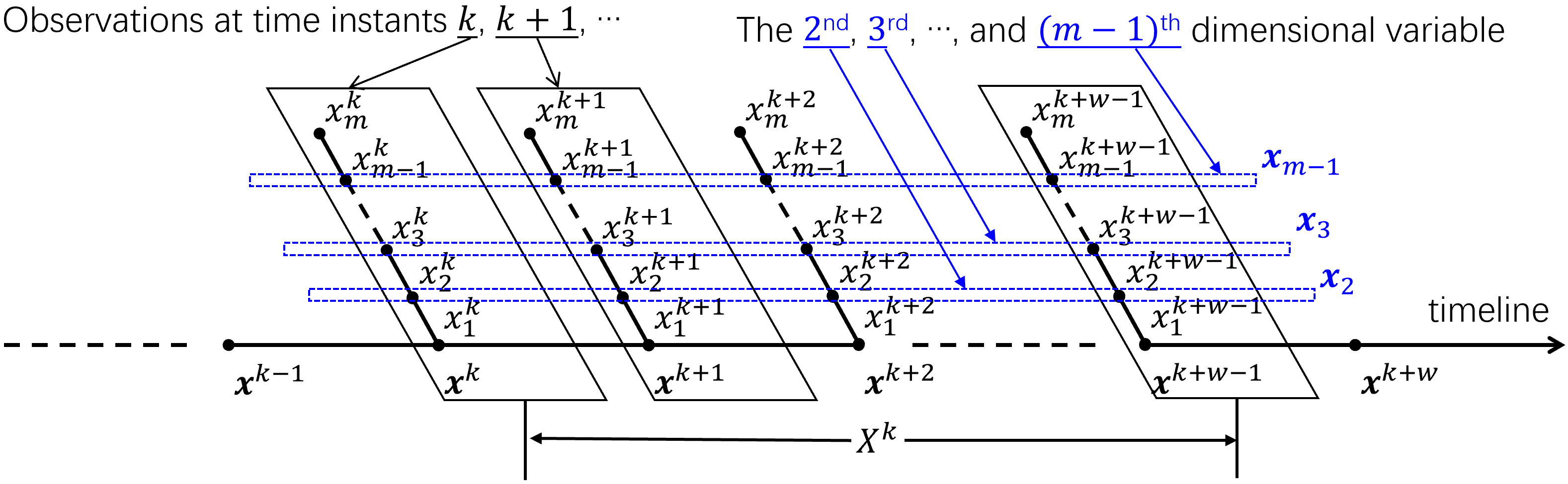
Figure 1: Local sample matrix with a sliding window of size $w$.

The general idea of our method is that $M$ contains all the nonlinear dependencies between any pairwise variables of the underlying fault process at time instant $k$. In a stationary environment, any quantities or statistics associated with $M$ should remain unchanged or stable. However, the existence of an abrupt fault may affect, at least, the values of one or more entries in the MI matrix, thus altering the values of our monitored quantities or statistics extracted from MI matrix.

Prior art suggests that those reliable quantities can be extracted from the orthogonal space spanned by eigenvectors of the sample covariance matrix (e.g., [6, 7, 11, 51, 24, 25, 26]). Motivated by this idea, suppose the eigenvalue decomposition of MI matrix is given by $M=P\Lambda P^{-1}$, where $P\in\mathbb{R}^{m\times m}$ is the matrix of eigenvectors and $\Lambda=\operatorname{diag}(\lambda_{1},\lambda_{2},\cdots,\lambda_{m})\in\mathbb{R}^{m\times m}$ is a diagonal matrix with eigenvalues on the main diagonal. Then, a new representation of $X$ (denote it $T$) in the orthogonal space spanned by column vectors in $P$ can be expressed as,

$$T=XP\triangleq\begin{bmatrix}\mathbf{t}^{k-w+1}\\ \mathbf{t}^{k-w+2}\\ \vdots\\ \mathbf{t}^{k}\end{bmatrix}\in\mathbb{R}^{w\times m}.$$ (9)

We term the column vectors of $T$ the mutual information based transform components (MI-TCs). The terminology of transform components (TCs) originates from [6, 7, 24] and is defined over the sample covariance matrix $C=\frac{1}{w-1}X^{T}X$. Specifically, suppose $P_{C}$ and $\Lambda_{C}$ are respectively the eigenvectors and eigenvalues of $C$, i.e., $C=P_{C}\Lambda_{C}{P_{C}}^{-1}$, then the original TCs of $X$ are given by $T_{C}=XP_{C}\in\mathbb{R}^{w\times m}$.

Compared with the MI matrix $M$, the covariance matrix $C$ only captures the linear dependence (correlation) between pairwise dimensions of the normalized measurement [24]. By contrast, the MI matrix $M$ operates with the full PDF information between pairs of variables and makes no assumption on the joint distribution of the measurement nor the nature of the relationship between pairwise dimensions. Moreover, it can simply identify nonlinear and non-monotonic dependencies [52], which are common in industrial process [10, 24, 26, 53]. See Fig. 2 for a few concrete examples on the advantage of MI over linear correlation, in which the linear correlation fails completely in quantifying nonlinear and non-monotonic effects (the bottom row).

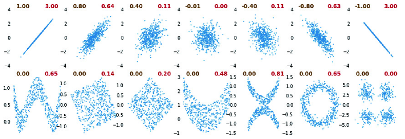
Figure 2: Examples of correlation versus mutual information (MI) estimated by the classic Shannon’s discrete entropy functional with the formula $H(\mathbf{x})=-\sum\limits_{x\in\mathbf{x}}p(x)\log_{2}p(x)$, over 500 samples. Each panel illustrates a scatter plot of samples drawn from a particular bivariate distribution. For each example, the correlation between the two variables is shown in brown (left) and the MI is shown in red (right). The top row shows linear relationships, for which MI and correlation both detect a relationship (although in different scales). The bottom row shows a series of distributions for which the correlation is $0$, but the MI is significant larger than $0$.

In each sliding window, we characterize $T$ with a detection index $\mathbf{\Theta}^{k}=[\mathbf{\mu}_{k}|\mathbf{\nu}_{k}|\mathbf{\zeta}_{k}|\mathbf{\gamma}_{k}]^{T}\in\mathbb{R}^{4m}$, it consists of the first-order statistic (i.e., the mean $\mathbf{\mu}_{k}=\mathbb{E}(\mathbf{t}^{k})$), the second-order statistic (i.e., the variance $\mathbf{\nu}_{k}=\mathbf{\sigma}_{k}^{2}=\mathbb{E}\left[({\mathbf{t}^{k}-\mathbf{\mu}_{k}})^{2}\right]$), the third-order statistic (i.e., the skewness $\mathbf{\zeta}_{k}=\mathbb{E}\left[\left(\frac{\mathbf{t}^{k}-\mathbf{\mu}_{k}}{\mathbf{\sigma}_{k}}\right)^{3}\right]$), and the forth-order statistic (i.e., the excess kurtosis $\mathbf{\gamma}_{k}=\mathbb{E}\left[\left(\frac{\mathbf{t}^{k}-\mathbf{\mu}_{k}}{\mathbf{\sigma}_{k}}\right)^{4}\right]-3$). Specifically, the empirical estimation to $\mathbf{\mu}_{k}$, $\mathbf{\nu}_{k}$, $\mathbf{\zeta}_{k}$ and $\mathbf{\gamma}_{k}$ are given by:

$$\mathbf{\mu}_{k}=\frac{1}{w}\sum_{i=0}^{w-1}\mathbf{t}^{k-i}\in\mathbb{R}^{1\times m},$$ (10)

$$\mathbf{\nu}_{k}=\frac{1}{w}\sum_{i=0}^{w-1}\left(\mathbf{t}^{k-i}-\mathbf{\mu}_{k}\right)^{2}\in\mathbb{R}^{1\times m},$$ (11)

$$\mathbf{\zeta}_{k}=\frac{1}{w\mathbf{\sigma}_{k}^{3}}\sum_{i=0}^{w-1}\left(\mathbf{t}^{k-i}-\mathbf{\mu}_{k}\right)^{3}\in\mathbb{R}^{1\times m},$$ (12)

$$\mathbf{\gamma}_{k}=\frac{1}{w\mathbf{\sigma}_{k}^{4}}\sum_{i=0}^{w-1}\left(\mathbf{t}^{k-i}-\mathbf{\mu}_{k}\right)^{4}-3\in\mathbb{R}^{1\times m}.$$ (13)

Note that, $\mathbf{\mu}^{*}=\mathbb{E}\left[\mu_{k}\right]$ (the mean of the TCs under normal condition) is used for the online calculation of detection index. When a fault occurs, one or more of the four statistics (namely, $\mathbf{\mu}_{k},\mathbf{\nu}_{k},\mathbf{\zeta}_{k}$ and $\mathbf{\gamma}_{k}$) are expected to deviate significantly from their expectations.

Given $\Theta^{k}$, a similarity index for local sample matrix $X^{k}$ at time instant $k$ can be defined as:

$$D^{k}=\|\Theta_{\sigma}^{-1}(\Theta^{k}-\Theta_{\mu})\|_{p},$$ (14)

where $\Theta_{\mu}$ denotes the mean value of similarity index over training data, $\Theta_{\sigma}=\operatorname{diag}(\sigma_{1},\sigma_{2},\cdots,\sigma_{4m})$ denotes a diagonal matrix in which the main diagonal consists of the standard deviation in each dimension of $\Theta^{k}$. The empirical method based on training data is used to determine the upper control limit $D_{\text{cl}}$ with a given confidence level $\eta$ [20]. An online monitoring procedure is then used to quantify the dissimilarity of statistics between normal and abnormal states.

Algorithm 1 and Algorithm 2 summarize, respectively, the offline training and the online testing of our proposed PMIM.

Algorithm 1 Fault detection using PMIM (training phase)

1:Process measurements $\aleph=\{\mathbf{x}^{i}|\mathbf{x}^{i}\in\mathbb{R}^{m}\}_{i=1}^{n}$; sliding window size $w$; significance level $\eta$.

2:mean of the transform components (TCs) $\mathbf{\mu}^{*}$; standard deviation $\Theta_{\sigma}$ of the detection index; reference mean $\Theta_{\mu}$ of the detection index.

3:for $i=1$ to $n$ do

4:    Construct a local time-lagged matrix $X^{i}\in\mathbb{R}^{w\times m}$ at time instant $i$ by Eq. (7);

5:    Construct the MI matrix $M^{i}$ by Eq. (8);

6:    Obtain the TCs $T^{i}$ of $X^{i}$ by Eq. (9);

7:    Obtain the detection index $\Theta^{i}=[\mathbf{\mu}_{i}|\mathbf{\nu}_{i}|\mathbf{\zeta}_{i}|\mathbf{\gamma}_{i}]^{T}$ by Eqs. (10)-(13).

8:end for

9:Calculate the mean of the TCs $\mathbf{\mu}^{*}=\sum\limits_{i=1}^{n}{\mathbf{\mu}_{i}}$, reference mean $\Theta_{\mu}$ and standard deviation $\Theta_{\sigma}$.

10:for $i=1$ to $n$ do

11:     $D^{i}=\|\Theta_{\sigma}^{-1}(\Theta^{i}-\Theta_{\mu})\|_{p}$.

12:end for

13:Determine the control limit $D_{\text{cl}}$ at the significance level $\eta$.

14:return $\mathbf{\mu}^{*}$; $\Theta_{\sigma}$; $\Theta_{\mu}$; $D_{\text{cl}}$

Algorithm 2 Fault detection using PMIM (testing phase)

1:The online process measurement $\{\mathbf{x}_{\text{test}}^{1},\mathbf{x}_{\text{test}}^{2},\cdots\}$; sliding window size $w$; mean of the transform components (TCs) $\mu^{*}$; standard deviation $\Theta_{\sigma}$ of the detection index; reference mean $\Theta_{\mu}$of the detection index; control limit $D_{\text{cl}}$.

2:Decision: alarm or not.

3:while End of process not reached do

4:    Construct a local time-lagged matrix $X_{\text{test}}^{i}\in\mathbb{R}^{w\times m}$ at time instant $i$ by Eq. (7);

5:    Construct the MI matrix $M_{\text{test}}^{i}$ by Eq. (8);

6:    Obtain the TCs $T_{\text{test}}^{i}$ of $X_{\text{test}}^{i}$ by Eq. (9);

7:    Obtain the detection index $\Theta_{\text{test}}^{i}=[\mathbf{\mu}_{i}|\mathbf{\nu}_{i}|\mathbf{\zeta}_{i}|\mathbf{\gamma}_{i}]_{\text{test}}^{T}$ with the mean of the TCs $\mathbf{\mu}^{*}$;

8:    Obtain the similarity index by $D_{\text{test}}^{i}=\|\Theta_{\sigma}^{-1}(\Theta_{\text{test}}^{i}-\Theta_{\mu})\|_{p}$;

9:    if $D_{\text{test}}^{i}\geq D_{\text{cl}}$ then

10:         Alarm the occurrence of fault;

11:         Identify the root variables that cause the fault;

12:    else

13:         $i=i+1$; Go back to Step 2.

14:    end if

15:end while

16:return Decision

4 A Deeper Insight into the Implementation of PMIM

In this section, we elaborate the implementation details of PMIM. The discussion is based on a synthetic process with time-correlated dynamics[24, 25]:

$$\mathbf{x}=A\mathbf{s}+\mathbf{e},$$ (15)

where $\mathbf{x}\in\mathbb{R}^{m}$ is the process measurements, $\mathbf{s}\in\mathbb{R}^{r}(r<m)$ is the data sources, $\mathbf{e}\in\mathbb{R}^{m}$ is the noise, and $A\in\mathbb{R}^{m\times r}$ is coefficient matrix that assumed to be column full rank [25, 16]. Let us assume data sources satisfy the following relations:

$$s^{k}_{i}=\sum_{j=1}^{l}\beta_{i,j}v^{k-j+1}_{i},$$ (16)

where $s^{k}_{i}$ is the $i$-th variable at time $k$, $v^{k-j+1}_{i}$ represents the value of the $i$-th Gaussian data source with time independence at time $k-j+1$, $\beta_{i,j}$ denotes the weight coefficient, $l\geq 2$. Obviously, both $\mathbf{s}$ and $\mathbf{x}$ are time-correlated.

Here, the fault type of sensor bias is considered:

$$\mathbf{x}^{*}=\mathbf{x}+\mathbf{f},$$ (17)

where $\mathbf{x}^{*}$ is the measurement under sensor bias, and $\mathbf{x}$ denotes the fault-free portion. In the following, we will show how $\mathbf{f}$ affects the matrix-based Rényi’s $\alpha$-order entropy.

The matrix-based Rényi’s $\alpha$-order entropy is a non-parametric measure of entropy. For the $p$-th variable with $w$ realizations, we build its Gram matrix $K\in\mathbb{R}^{w\times w}$ (at time instant $k$) by projecting it into a RKHS with an infinite divisible kernel:

$$\centering K_{\mathbf{x}_{p}}=\begin{bmatrix}1&\exp\!\left(\!-\frac{(x^{k-w+1}_{p}-x^{k-w+2}_{p})^{2}}{2\sigma^{2}}\!\right)\!&\cdots&\exp\!\left(\!-\frac{(x^{k-w+1}_{p}-x^{k}_{p})^{2}}{2\sigma^{2}}\!\right)\!\\ \exp\!\left(\!-\frac{(x^{k-w+2}_{p}-x^{k-w+1}_{p})^{2}}{2\sigma^{2}}\!\right)\!&1&\cdots&\exp\!\!\left(\!\!-\frac{(x^{k-w+2}_{p}-x^{k}_{p})^{2}}{2\sigma^{2}}\!\right)\!\\ \vdots&\vdots&\ddots&\vdots\\ \exp\!\left(\!-\frac{(x^{k}_{p}-x^{k-w+1}_{p})^{2}}{2\sigma^{2}}\!\right)\!&\exp\!\left(\!-\frac{(x^{k}_{p}-x^{k-w+2}_{p})^{2}}{2\sigma^{2}}\!\right)\!&\cdots&1\\ \end{bmatrix}.\@add@centering$$ (18)

We normalize $K$ by its trace, i.e., $K=K/{\text{tr}(K)}$. It should be noted that the kernel induced mapping can be understood as a means of computation of high order statistics.

Suppose the fault occurs exactly at the $p$-th variable, i.e., $\mathbf{x}_{p}^{*}=\mathbf{x}_{p}+\mathbf{f}$ and $\mathbf{f}=\{f^{k-w+1},f^{k-w+2},\cdots,f^{k}\}$. The $(i,j)$-th entry of the Gram matrix $K$ associated with $\mathbf{x}_{p}$ becomes:

$$\begin{split}\exp\!\left(\!-\frac{||x_{p}^{i*}-x_{p}^{j*}||^{2}}{2\sigma^{2}}\!\right)\!&=\exp\!\left(\!-\frac{[(x_{p}^{i}+f^{i})-(x_{p}^{j}+f^{j})]^{2}}{2\sigma^{2}}\!\right)\!\\ &=\exp\!\left(\!-\frac{[(x_{p}^{i}-x_{p}^{j})+(f^{i}-f^{j})]^{2}}{2\sigma^{2}}\!\right)\!\\ &=\exp\!\left(\!-\frac{(x_{p}^{i}-x_{p}^{j})^{2}}{2\sigma^{2}}\!\right)\!\exp\!\left(\!-\frac{(x_{p}^{i}-x_{p}^{j})(f^{i}-f^{j})}{\sigma^{2}}\!\right)\!\exp\!\left(\!-\frac{(f^{i}-f^{j})^{2}}{2\sigma^{2}}\!\right)\!,\\ \end{split}$$ (19)

where $i$, $j$ are time indices. Therefore, the new Gram matrix $K_{\mathbf{x}_{p}}^{*}$ can be represented as:

$$K_{\mathbf{x}_{p}}^{*}=K_{\mathbf{x}_{p}}\circ K_{\langle\mathbf{x}_{p},~{}\mathbf{f}\rangle}\circ K_{\mathbf{f}}\\ ,$$ (20)

where

$$\begin{split}&K_{\langle\mathbf{x}_{p},~{}\mathbf{f}\rangle}=\\ &\begin{bmatrix}1&\exp\!\!\left(\!\!-\frac{(x_{p}^{k-w+1}-x_{p}^{k-w+2})(f^{k-w+1}-f^{k-w+2})}{\sigma^{2}}\!\!\right)\!\!&\cdots&\exp\!\!\left(\!\!-\frac{(x_{p}^{k-w+1}-x_{p}^{k})(f^{k-w+1}-f^{k})}{\sigma^{2}}\!\!\right)\!\!\\ \exp\!\!\left(\!\!-\frac{(x_{p}^{k-w+2}-x_{p}^{k-w+1})(f^{k-w+2}-f^{k-w+1})}{\sigma^{2}}\!\!\right)\!\!&1&\cdots&\exp\!\!\left(\!\!-\frac{(x_{p}^{k-w+2}-x_{p}^{k})(f^{k-w+2}-f^{k})}{\sigma^{2}}\!\!\right)\!\!\\ \vdots&\vdots&\ddots&\vdots\\ \exp\!\!\left(\!\!-\frac{(x_{p}^{k}-x_{p}^{k-w+1})(f^{k}-f^{k-w+1})}{\sigma^{2}}\!\!\right)\!\!&\exp\!\!\left(\!\!-\frac{(x_{p}^{k}-x_{p}^{k-w+2})(f^{k}-f^{k-w+2})}{\sigma^{2}}\!\!\right)\!\!&\cdots&1\\ \end{bmatrix}\\ \end{split},$$ (21)

and

$$\begin{split}K_{\mathbf{f}}&=\begin{bmatrix}1&\exp\!\left(\!-\frac{(f^{k-w+1}-f^{k-w+2})^{2}}{2\sigma^{2}}\!\right)\!&\cdots&\exp\!\left(\!-\frac{(f^{k-w+1}-f^{k})^{2}}{2\sigma^{2}}\!\right)\!\\ \exp\!\left(\!-\frac{(f^{k-w+2}-f^{k-w+1})^{2}}{2\sigma^{2}}\!\right)\!&1&\cdots&\exp\!\left(\!-\frac{(f^{k-w+2}-f^{k})^{2}}{2\sigma^{2}}\!\right)\!\\ \vdots&\vdots&\ddots&\vdots\\ \exp\!\left(\!-\frac{(f^{k}-f^{k-w+1})^{2}}{2\sigma^{2}}\!\right)\!&\exp\!\left(\!-\frac{(f^{k}-f^{k-w+2})^{2}}{2\sigma^{2}}\!\right)\!&\cdots&1\\ \end{bmatrix}\\ \end{split}.$$ (22)

In case of incipient faults, $f^{i}-f^{j}\approx 0$, Eq. (22) reduces to an all-ones matrix. As a result, Eq. (20) can be approximated with $K_{\mathbf{x}_{p}}^{*}\approx K_{\mathbf{x}_{p}}\circ K_{\langle\mathbf{x}_{p},~{}\mathbf{f}\rangle}$. Take the simulation data described in section 5.1 as an example, $\mathbf{f}$ is induced on $\mathbf{x}_{1}$, the Gram matrix of $\mathbf{x}_{1}$ and $\mathbf{x}_{1}^{*}$ , i.e., $K_{\mathbf{x}_{1}}$ and $K_{\mathbf{x}_{1}}^{*}$, are shown in Fig. 3. As can be seen, the incipient fault $\mathbf{f}$ causes minor changes on the (normalized) Gram matrix as well as its eigenspectrum, and thus the entropy of the variable.

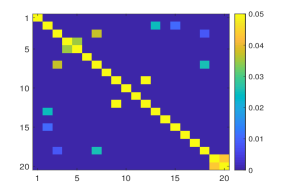
(a) $K_{\mathbf{x}_{1}}$

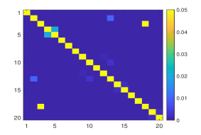
(b) $K_{\mathbf{x}_{1}}^{*}$

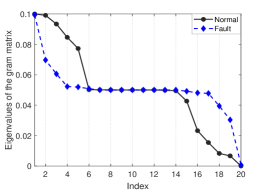
(c) $Eigenvalues$

Figure 3: The (normalized) Gram matrix and its associated eigenspectrum in normal state or under incipient fault. (a) $K_{\mathbf{x}_{1}}$ in normal state; (b) $K_{\mathbf{x}_{1}}^{*}$ under incipient fault; (c) the eigenspectrum of $K_{\mathbf{x}_{1}}$ and $K_{\mathbf{x}_{1}}^{*}$. The incipient fault causes an obvious change in eigenspectrum, and thus the entropy of data.

We now discuss the change of MI between the $p$-th variable $\mathbf{x}_{p}$ and the $q$-th variable $\mathbf{x}_{q}$. Again, suppose the fault of sensor bias occurs at the $p$-th variable $\mathbf{x}_{p}^{*}$, the difference between $I(\mathbf{x}_{p};\mathbf{x}_{q})$ and $I(\mathbf{x}_{p}^{*};\mathbf{x}_{q})$ is:

$$\begin{split}\triangle I(\mathbf{x}_{p}^{*};\mathbf{x}_{q})&=I(\mathbf{x}_{p}^{*};\mathbf{x}_{q})-I(\mathbf{x}_{p};\mathbf{x}_{q})\\ &=[H_{\alpha}(A_{p}^{*})+H_{\alpha}(A_{q})-H_{\alpha}(A_{p}^{*},A_{q})]-[H_{\alpha}(A_{p})+H_{\alpha}(A_{q})-H_{\alpha}(A_{p},A_{q})]\\ &=H_{\alpha}(A_{p}^{*})-H_{\alpha}(A_{p}^{*},A_{q})-H_{\alpha}(A_{p})+H_{\alpha}(A_{p},A_{q})\\ &=\frac{1}{1-\alpha}\log_{2}\left(\frac{\sum\limits_{i=1}^{w}\lambda_{i}(A_{p}^{*})^{\alpha}\sum\limits_{i=1}^{w}\lambda_{i}\left(\frac{A_{p}\circ A_{q}}{\operatorname{tr}(A_{p}\circ A_{q})}\right)^{\alpha}}{\sum\limits_{i=1}^{w}\lambda_{i}(A_{p})^{\alpha}\sum\limits_{i=1}^{w}\lambda_{i}\left(\frac{A_{p}^{*}\circ A_{q}}{\operatorname{tr}(A_{p}^{*}\circ A_{q})}\right)^{\alpha}}\right),\\ \end{split}$$ (23)

where $\lambda_{i}(A)$ denotes the $i$-th eigenvalue of matrix $A$, the normalized Gram matrix obtained from the corresponding variable.

Again, we use the simulated data described in section 5.1 as an example, where the fault is induced in $\mathbf{x}_{1}$. By comparing the MI matrix under normal and fault states, as shown in Fig. 4, we can observe that all entries related to $\mathbf{x}_{1}$ (the first dimensional measurement) have a sudden change. For example, the MI value in $M_{12}$ is $2.51$ under normal state, but it becomes $2.67$ with incipient fault. This result also indicates that our methodology has the potential to identify the exact fault sources by monitoring significant changes in MI values over MI matrix, which makes our detection result interpretable.

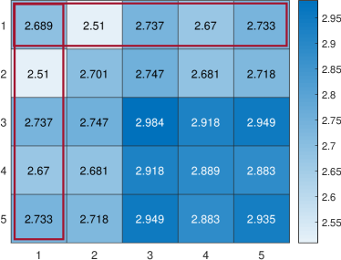
(a) Normal

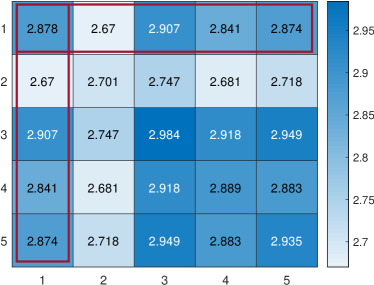
(b) Fault

Figure 4: The MI matrix under (a) normal state; and (b) fault state (the fault is induced on $\mathbf{x}_{1}$). The entries with changed values are marked with red rectangles. Only entries that are related to $\mathbf{x}_{1}$ have different MI values.

5 Experiments

In this section, experiments on both synthetic data and the real-world Tennessee Eastman process (TEP) are conducted to demonstrate the superiority of our proposed PMIM over state-of-the-art fault detection methods. We also evaluate the robustness of PMIM with respect to different hyper-parameter settings.

Two generally used metrics, namely the fault detection rate (FDR) and the false alarm rate (FAR), are employed for performance evaluation[1, 54, 55]. The FDR is the probability of event where an alarm is raised when a fault really occurs,

$$\text{FDR}=\text{prob}(D>D_{\text{cl}}|\text{fault $\neq$ 0}),\\$$ (24)

where $D$ and $D_{\text{cl}}$ are respectively the similarity index and its corresponding control limit. By contrast, the FAR is the percentage of the samples under normal state but are identified as faults,

$$\text{FAR}=\text{prob}(D>D_{\text{cl}}|\text{fault = 0}).\\$$ (25)

Obviously, a higher FDR and a lower FAR is expected.

5.1 Numerical Simulation

Motivated by [16, 24, 25], we consider a multivariate nonlinear process generated by the following equation:

$$\begin{bmatrix}x_{1}\\ x_{2}\\ x_{3}\\ x_{4}\\ x_{5}\\ \end{bmatrix}=\begin{bmatrix}{0.2183}&{-0.1693}&{0.2063}\\ {-0.1972}&{0.2376}&{0.1736}\\ {0.9037}&{-0.1530}&{0.6373}\\ {0.1146}&{0.9528}&{-0.2624}\\ {0.4173}&{-0.2458}&{0.8325}\\ \end{bmatrix}\begin{bmatrix}{s_{1}}^{2}\\ s_{2}s_{3}\\ {s_{3}}^{3}\\ \end{bmatrix}+\begin{bmatrix}e_{1}\\ e_{2}\\ e_{3}\\ e_{4}\\ e_{5}\\ \end{bmatrix},$$

where $s$ satisfies $s^{k}_{i}=\sum_{j=1}^{l}\beta_{i,j}v^{k-j+1}_{i}$ with a weight matrix $\mathbf{\beta}$ given by,

$$\mathbf{\beta}=\begin{bmatrix}{0.6699}&{0.0812}&{0.5308}&{0.4527}&{0.2931}\\ {0.4071}&{0.8758}&{0.2158}&{-0.0902}&{0.1122}\\ {0.3035}&{0.5675}&{0.3064}&{0.1316}&{0.6889}\\ \end{bmatrix},$$

$v$ denotes three mutually independent Gaussian distributed data sources with mean of $[0.3,~{}2.0,~{}3.1]^{T}$ and standard deviation of $[1.0,~{}2.0,~{}0.8]^{T}$, and $e$ denotes Gaussian white noises with standard deviation $[0.061,~{}0.063,~{}0.198,~{}0.176,~{}0.170]^{T}$. Same to [24, 25], we consider four different types of faults that cover a broad spectrum of real-life scenarios,

• Type I: Sensor bias $\mathbf{x}^{*}=\mathbf{x}+f$, with $f=5.6+\mathbf{e}$, $\mathbf{e}$ randomly chosen from [0, 1.0];

• Type II: Sensor precision degradation $\mathbf{x}^{*}=\eta\mathbf{x}$ with $\eta=0.6$;

• Type III: Additive process fault $\mathbf{s}^{*}=\mathbf{s}+f$ with $f=1.2$;

• Type IV: Dynamic changes $\mathbf{\tilde{\beta}}=\mathbf{\beta}+\bigtriangleup\mathbf{\beta}$ with $\bigtriangleup\beta_{3}=[-0.825,~{}0.061,~{}0.662,~{}-0.820,~{}0.835]$, where $\mathbf{\beta}_{3}$ denotes the $3$-th row of $\mathbf{\beta}$.

The training set contains $10,000$ samples, the test set contains $4,000$ samples. All the faults are introduced after the $1,000$-th sample. For convenience, we assume sensor fault occurs at $\mathbf{x}_{1}$ (i.e., the first dimension of observable measurement), and process fault occurs at $\mathbf{s}_{1}$ (i.e., the first independent data sources). Empirical evaluation aims to answer the following three questions:

• Can MI manifest more complex dependence among different dimensions of measurement than the classical correlation coefficient?

• Is fault detection using PMIM robust to hyper-parameter settings and how hyper-parameters affect the performance of PMIM?

• Does PMIM outperform existing state-of-the-art window-based fault detection methods?

5.1.1 MI versus Pearson’s correlation coefficient

Firstly, we demonstrate the advantage of MI over the Pearson’s correlation coefficient $\gamma$ on manifesting the complex (especially nonlinear) dependency between two variables. Intuitively, if two random variables are linearly correlated, they should have large $\gamma^{2}$ ($\gamma^{2}>0.6$) and large MI(but we cannot compare the value of $\gamma^{2}$ to the value of MI). However, if they are related in a nonlinear fashion, they should have large MI but small $\gamma^{2}$ ($\gamma^{2}\leq 0.6$) [33]. On the other hand, two variables will never have a large $\gamma^{2}$ but a small MI, as linear correlation is a very special case of the general dependence. Therefore, MI should always be a superior metric to measure the degree of interactions than Pearson’s correlation coefficient. We perform a simple simulation to support our argument.

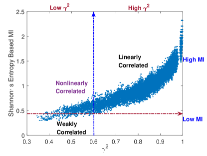
(a) Shannon’s MI versus $\gamma^{2}$

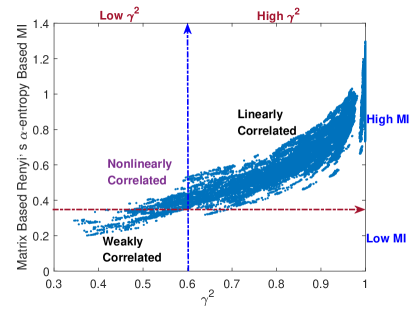
(b) Matrix-based Rényi’s $\alpha$-order MI versus $\gamma^{2}$

Figure 5: The comparison between Pearson’s correlation coefficient $\gamma^{2}$ and mutual information estimated with (a) Shannon’s discrete entropy functional by discretizing continuous variables into $5$ bins of equal width; and (b) matrix-based Rényi’s $\alpha$-order MI. The values of $\gamma^{2}$ and MI are shown in $x$-axis and $y$-axis, respectively.

Specifically, we select the first $4,000$ samples in the training set and compute both MI and $\gamma^{2}$ in each window data of size $100$. We finally obtain $3,601$ pairs of MI and $\gamma^{2}$. We evaluate MI with both the basic Shannon’s discrete entropy functional and our suggested matrix-based Rényi’s $\alpha$-order entropy functional. For Shannon entropy functional, we discretize continuous variables into $5$ bins of equal width to estimate the underlying distributions. The values of MI ($y$-axis) and $\gamma^{2}$ ($x$-axis) are specified in the scatter plot in Fig. 5. As can be seen, there are strong nonlinear dependencies in our simulated data. Take Fig. 5(b) as an example, we can observe that when $\gamma^{2}=0.6$, the smallest MI is $0.37$. As such, we consider $MI\geq 0.37$ to indicate a strong correlation. We noticed that there are quite a few points in the region $0.37\leq MI\leq 1.2$ and $\gamma^{2}\leq 0.6$, suggesting that nonlinear dependence dominates for a large number of variables.

Further, to quantitatively demonstrate the superiority of MI matrix over the well-known covariance matrix on nonlinear fault detection, we use MI matrix as a substitute to the covariance matrix in the basic PCA-based fault detection approach. We denote this simple modification as MI-PCA, which includes both MI-PCA${}_{\text{Shannon}}$ and MI-PCA${}_{\text{R{\'{e}}nyi}}$. Both Hotelling $T^{2}$ and squared prediction error (SPE) are considered in PCA and MI-PCA. Performances in terms of FDR and FAR are shown in Fig. 6. In case of $T^{2}$, MI-PCA always has higher or almost the same FDR values, but significantly smaller FAR values. In case of SPE, although traditional PCA has smaller FAR, its results are meaningless. In fact, if we look deeper, the FDR of PCA is almost zero, which suggests that traditional PCA completely fails.

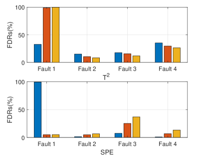
(a) FDRs

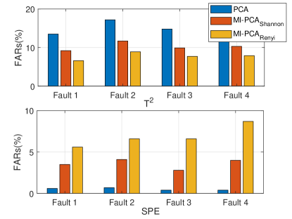
(b) FARs

Figure 6: Performance comparison between PCA and MI-PCA in terms of FDR (the larger the better) and FAR (the smaller the better). We replace the covariance matrix in the basic PCA-based fault detection with MI matrix estimated with both Shannon entropy (denote it MI-PCA${}_{\text{Shannon}}$) and matrix based Rényi’s $\alpha$-order entropy (denote it MI-PCA${}_{\text{R{\'{e}}nyi}}$). We use both Hotelling $T^{2}$ and squared prediction error (SPE) to monitor the state of samples.

5.1.2 Hyperparameter analysis

We then present a comprehensive analysis on the effects of three hyper-parameters, namely the entropy order $\alpha$, the kernel size $\sigma$ and the length $w$ of sliding window in PMIM. We focus our discussion on the process data with time-correlated dynamic changes, i.e., fault Type V. The FDR and FAR values of our methodology with respect to different hyper-parameter settings are shown in Fig. 7, Fig. 8 and Fig. 9.

The choice of $\alpha$ is associated with the task goal. If the application requires emphasis on tails of the distribution (rare events) or multiple modalities, $\alpha$ should be less than 2, but if the goal is to characterize modal behavior, $\alpha$ should be greater than 2. $\alpha=2$ provides neutral weighting [46, 57]. The detection performances of different values of $\alpha$ are presented in Fig. 7. For a comprehensive comparison, we consider $\alpha\in\{0.1,~{}0.2,~{}0.3,~{}0.4,~{}0.5,~{}0.6,~{}0.7,~{}0.8,~{}0.9,~{}1,$ $~{}1.1,~{}1.2,~{}1.3,~{}1.4,~{}1.5,~{}2,~{}3,~{}5\}$. Both $\ell_{\infty}$ and $\ell_{2}$ are assessed in the calculation of similarity index $D$ in Eq. (14). As a common practice, we use window size $100$. As can be seen, the FDR values are always larger than $99.5\%$, which suggests that FDR is less sensitive to the changes of $\alpha$. On the other hand, the FAR keeps a stable value in the range $\alpha\in[0.5,~{}1.2]$, but suddenly increases to $25\%$ or above when $\alpha\geq 2$. Therefore, we recommend $\alpha$ in the range $[0.5,~{}1.2]$ for PMIM.

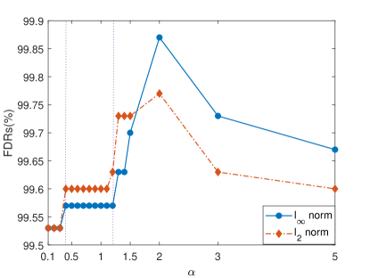
(a) FDRs with different $\alpha$

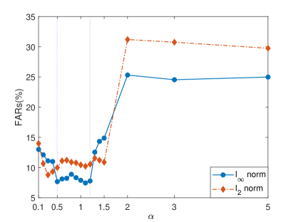
(b) FARs with different $\alpha$

Figure 7: Detection performances of different $\alpha$ on (a) FDRs; and (b) FARs. Both $\ell_{\infty}$ and $\ell_{2}$ norm are considered in the calculation of similarity index $D$. As a common practice, window size $100$ is used here.

The parameter $\sigma$ controls the locality of the estimator, its selection can follow Silverman’s rule of thumb for density estimation [58] or other heuristics from a graph cut perspective (e.g., the $10$ to $30$ percent of the total range of the Euclidean distances between all pairwise data points [59]). For example, the range from a graph cut perspective corresponds to $0.21<\sigma<1.33$ on the normalized data here. The detection performances of different $\sigma$ and $\alpha$ are presented in Fig. 8. We choose $\sigma\in\{0.1,~{}0.2,~{}0.3,~{}0.4,~{}0.5,~{}0.6,$ $~{}0.7,~{}0.8,~{}0.9,~{}1,~{}5,~{}10,~{}24,~{}50,~{}100\}$ (displayed in log-scale) and $\alpha\in\{0.4,~{}0.5,$ $~{}0.6,~{}0.7,~{}0.8,~{}0.9,~{}1,~{}1.1,~{}1.2,~{}1.5\}$. According to Fig. 8, FDR is always larger than $99.20\%$, whereas FAR is relatively more sensitive to $\sigma$. Specifically, FAR reaches to its minimum value when $\sigma$ is around $0.5$. After that, FAR is consistently increasing when $\sigma\in[1,~{}100]$. To achieve higher FDR and lower FAR values, we thus recommend $\sigma$ in the range $[0.4,~{}1]$ for PMIM.

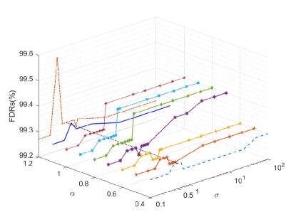
(a) FDRs with different $\sigma$

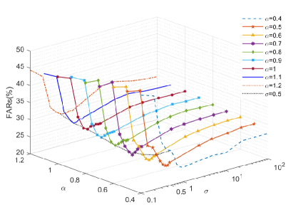
(b) FARs with different $\sigma$

Figure 8: Detection performances of different $\sigma$ with a fixed $\alpha$ on (a) FDRs; and (b) FARs. $\sigma\in\{0.1,~{}0.2,~{}0.3,~{}0.4,$ $~{}0.5,~{}0.6,~{}0.7,~{}0.8,$ $~{}0.9,~{}1,~{}5,~{}10,~{}24,~{}50,~{}100\}$ (displayed in log-scale). $\ell_{2}$ norm is considered in the calculation of similarity index $D$.

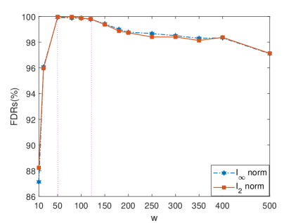
(a) FDRs with different $w$

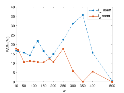
(b) FARs with different $w$

Figure 9: Detection performances of different $w$ on (a) FDRs; and (b) FARs. Both $\ell_{\infty}$ and $\ell_{2}$ norm are considered for scalarization in the calculation of similarity index $D$.

The local stationarity or smoothness assumption (of the underlying process) might be violated if the window size is too large. In this case, the eigenspectrum becomes stable and is less sensitive to the abrupt distributional changes of the underlying process, which may lead to decreased detection power or lower FDR values. On the other hand, in case of a very small window size, the MI estimation becomes unreliable (due to limited samples) and the local time-lagged matrix may be dominated by environmental noises, which in turn would result in a high FAR value. Moreover, according to Fig. 9, FDR remains stable when $w\in[50,~{}120]$, and decreases as the window length increasing when $w\geq 120$. By contrast, FAR is more sensitive to $w$ than FDR, but its changing patterns are not consistent for $\ell_{2}$ norm and $\ell_{\infty}$ norm. We choose $w=100$ in the following experiments, because it can strike a good trade-off between FDR and FAR for both $\ell_{2}$ norm and $\ell_{\infty}$ norm here.

5.1.3 Comparison with state-of-the-art methods

We compare our proposed PMIM with four state-of-the-art window based data-driven fault detection approaches, namely DPCA [11], SPA [20], RTCSA [24] and RDTCSA [25]. The hyperparameters of PMIM are set to $\alpha=1.01$, $\sigma=0.5$ and $w=100$. For DPCA, $90\%$ cumulative percent variance is used to determine the number of principal components. For RTCSA, RDTCSA and PMIM, their detection performances are illustrated in Table 1 and Table 2.

Table 1: The FDRs $(\%)$ of different methods for the numerical simulations

No.	DPCA		SPA		RTCSA	RDTCSA	PMIM
	$T^{2}$	SPE	$D_{r}$	$D_{p}$
1	51.17	99.70	0.80	2.80	88.43	91.01	91.57
2	21.23	21.0	2.40	6.67	82.50	100	99.63
3	33.10	99.83	0.77	7.37	96.60	96.83	97.50
4	81.23	85.57	29.13	99.13	99.70	99.70	99.87
Aver.	46.68	76.53	8.28	29.0	91.81	96.89	97.14

• $T^{2}$ denotes Hotelling’s $T^{2}$ statistic; SPE denotes squared prediction error; $D_{r}$ and $D_{p}$ denote SPE and $T^{2}$ of statistics patterns (SPs) in SPA framework, respectively. For SPA, the selected statistics are mean, variance, skewness, and kurtosis. For DPCA, SPA and RDTCSA, the time lag is set to 2, 1 and 1 respectively. The window lengths are all set as the commonly used 100. For RTCSA, RDTCSA and PMIM, $\ell_{2}$ norm is used as scalarization. The significance level is set as 5%.

Table 2: The FARs $(\%)$ of different methods for the numerical simulations

No.	DPCA		SPA		RTCSA	RDTCSA	PMIM
	$T^{2}$	SPE	$D_{r}$	$D_{p}$
1	17.31	18.28	0.22	10.32	6.22	3.11	1.78
2	20.20	19.44	0	0	4.67	1.44	5.01
3	18.28	15.53	0	9.54	4.88	3.65	2.77
4	19.44	17.92	0	15.54	11.88	15.53	2.77
Aver.	18.81	17.79	0.055	8.85	6.91	5.93	3.08

According to Table 1, PMIM can effectively detect different types of faults and has the highest detection rate. Our advantage becomes more obvious for fault Type III and fault Type V, namely the additive process fault and dynamic changes. Moreover, as demonstrated in Table 2, for each test process, PMIM achieves smaller FAR values at the early stage of the normal phase. Although SPA achieves nearly zero FAR values, its FDR values is too small, which indicates that SPA is hard to identify faults here. This is not hard to understand. Note that SPA uses a time lag of $1$. In this sense, any two adjacent windows of data only differ in $1$ sample. The highly overlapped windows will lead to highly correlated SPs, which severely deteriorate the capability of SPA [20].

5.2 TEP Experiment

As a public benchmark of chemical industrial process, Tennessee Eastman process (TEP) created by the Eastman Chemical Company has been widely used for multivariable process control problems [60, 61] (see Appendix B on the introduction of TEP process). In this application, we use the simulation data generated by the closed-loop Simulink models developed by Braatz [61, 62, 63] to evaluate the effectiveness of our proposed PMIM. We use $22$ continuous process measurements (sampled with a sampling interval of 3 minutes) and $11$ manipulated variables (generated at time delay that varys from 6 to 15 minutes) for monitoring, which constitutes $33$ dimensional of input data. To obtain a reliable significance level, we generate $200$ hours of training data ($4,000$ samples in total) and $100$ hours of testing data ($2,000$ samples in total). In each test data, a fault occurs exactly after $20$ hours from the beginning.

First, the MI matrix (with the boxplot of its diagonal vector) of normal state, fault 1 (step fault) and fault 14 (sticking fault) are shown in Fig. 10. Obviously, the MI matrix keeps almost the same in different time instants under the normal state. However, the occurrence of a fault will lead to different joint or marginal distributions on each dimensional of input, and thus change the entry values in MI matrix. By comparing the boxplots of normal and fauts states, we can observe the changes of diagonal vector, i.e., changes of entropy. Moreover, different types of faults produce different changes of MI matrix.

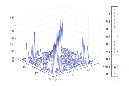
(a) Normal (t=$500$)

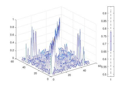
(b) Normal (t=$1,500$)

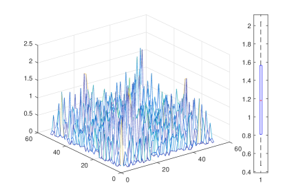
(c) Fault 1 (t=$1,500$)

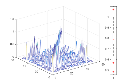
(d) Fault 14 (t=$1,500$)

Figure 10: The MI matrix of TEP under normal and fault states: (a) the MI matrix of normal state at $500$-th sampling instant; (b) the MI matrix of normal state at $1,500$-th sampling instant; (c) the MI matrix of fault 1 at $1,500$-th sampling instant; and (d) the MI matrix of fault 14 at $1,500$-th sampling instant.

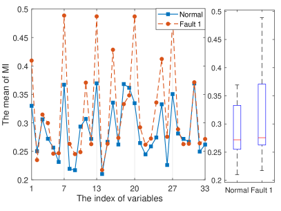
(a) Fault 1

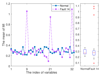
(b) Fault 14

Figure 11: The means of MI matrix of TEP under fault states: (a) fault 1 (step fault); and (b) fault 14 (sticking fault). The left plot is the means of MI along each variable, and the right is their confidence interval.

The mean of MI values between one variable and all remaining variables are shown in Fig. 11. As Fig. 11(a) shown, the central box becomes wider and the $75$-th percentiles becomes larger. This indicates that the fault 1 is possibly a step change. In fact, fault 1 indeed induce a step change on stream 4. This feeding changes of reactants A, B and C causes a global impacts on measurements. By contrast, fault 14 induces a sticking change on the reactor cooling water valve, and the most relevant variables are in dimensions $9$, $21$ and $32$ [62]. From Fig. 11(b), there are indeed three outliers which are plotted individually using the $``+"$ symbol, corresponding to the $9$-th, $21$-th and $32$-th dimensional variables. In other words, the changes on the dimensions $9$, $21$ and $32$ are exactly the driving force that lead to the changes in MI matrix (and hence its eigenspectrum). In this sense, our PMIM also provides insights on the exact root variables that cause the fault, i.e., our fault detection using PMIM is interpretable. One should also note that, an interpretable results also benefit problems related to fault isolation [64] and restoration [65].

Next, we use the empirical method to determine the confidence limits of different MSPM methods under the same confidence level. Without loss of generality, the window lengths of all competing methods are set to $100$, and all the statics mentioned in Section 3 are used here. The average FDR and FAR values of different MSPM methods on TEP are summarized in Table 3 and Table 4, respectively.

It can be observed from Table 3 that the FDR of RTCSA, RDTCSA, and PMIM are consistently higher than other methods and remain stable across different types of faults. Moreover, our PMIM always outperforms RTCSA, owing to the superiority of MI over covariance matrix in capturing the intrinsic interactions (either linear or non-linear) between pairwise variables. PMIM detects most of faults. Although our method has relatively lower FDR on step fault 5 and unknown fault 19 with $w=100$, its detection performance in both faults can be significantly improved with larger window size $w$ (see Fig. 12.) Detection performances in terms of FDR of different $w$ for fault 5 and 19 are shown in Fig. 12. $w=150$ is better to achieve higher FDRs here.

Table 3: The FDRs $(\%)$ of different MSPM methods for TEP

No.	DPCA		SPA		RTCSA	RDTCSA	PMIM
(fault type)	$T^{2}$	SPE	$D_{r}$	$D_{p}$
1 Step	99.91	99.94	99.88	99.81	99.62	99.56	99.69
2 Step	99.19	98.88	99.12	99.12	98.50	98.69	98.31
4 Step	11.63	100	16.50	100	98.38	99.44	99.56
5 Step	14.94	28.56	19.50	87.81	99.88	97.25	77.38
6 Step	99.50	100	13.63	13.63	100	99.94	100
7 Step	100	100	44.12	100	100	100	100
8 Random	98.88	93.63	99.12	99.12	97.88	97.75	98.62
10 Random	21.69	51.62	59.56	88.12	96.63	37.38	96.06
11 Random	36.88	95.44	99.69	100	96.25	92.94	99.0
12 Random	99.38	97.31	99.31	99.31	99.38	99.50	100
13 Slow drift	98.56	92.31	98.31	100	97.88	98.0	98.25
14 Sticking	99.88	99.94	99.94	99.94	99.88	99.88	99.88
16 Unknown	15.37	52.38	63.56	91.81	99.75	79.31	99.50
17 Unknown	87.19	98.31	98.0	99.31	97.81	97.75	97.88
18 Unknown	94.56	95.75	93.81	95.56	93.75	93.69	94.69
19 Unknown	48.25	49.75	29.38	99.62	100	97.19	78.19
20 Unknown	47.38	61.31	96.19	96.75	96.69	95.81	96.31

• The window lengths are all set as 100. The selected statistics are mean, variance, skewness, and kurtosis. For RTCSA, RDTCSA and PMIM, $\ell_{\infty}$ norm is used as scalarization. For DPCA and RDTCSA, the time lag is set to 2 and 1 respectively, recommended by authors [24, 25]. The significance level is set as 2%.

Table 4: The average FARs $(\%)$ of different MSPM methods for TEP

FAR	DPCA		SPA		RTCSA	RDTCSA	PMIM
$(\%)$	$T^{2}$	SPE	$D_{r}$	$D_{p}$
Normal	2.05	3.95	4.73	5.96	2.89	3.63	1.18

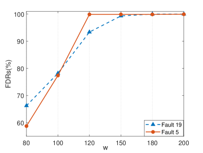
Figure 12: Detection performances in terms of FDR of different $w$ for fault 5 and 19 in TEP. $w\in\{80,~{}100,~{}120,$ $~{}150,180,200\}$. Fault 5 is marked by red, fault 19 is marked by blue.

From Table 4 all the methods achieve favorable FAR, approaching to the theoretical minimum value, i.e., the used significance level. Moreover, our FAR is lower than RTCSA and RDTCSA. This result confirms the superiority of MI in capturing the intrinsic interactions. On the other hand, the detection delay is inevitable owing to the use of sliding windows, a common drawback of the window-based MSPM methods. Take fault 1 for instance, detection performances in terms of FAR, FDR and TFDR (we define the FDR value in the transition phase as TFDR, the higher the better), of RTCSA, RDTCSA and PMIM are illustrated in Fig. 13. Our proposed PMIM has the lowest FAR and highest TFDR, which indicates that PMIM is more sensitive to fault 1 than RTCSA and RDTCSA. The detection delay of the proposed method is only 4 samples, which is acceptable in window-based approaches.

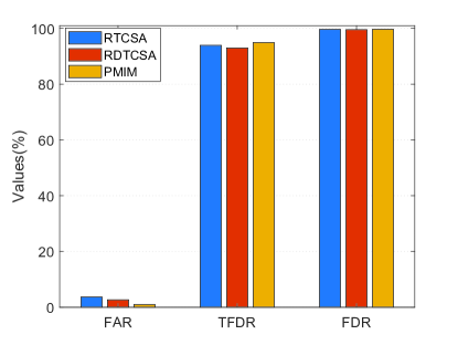
Figure 13: Detection performances of TCSA methods for fault 1 in TEP. TFDR refers to the FDR value in transition phase. The higher TFDR, the better performance of the used methodology. The methods of RTCSA, RDTCSA and PMIM are marked by blue, red and yellow respectively.

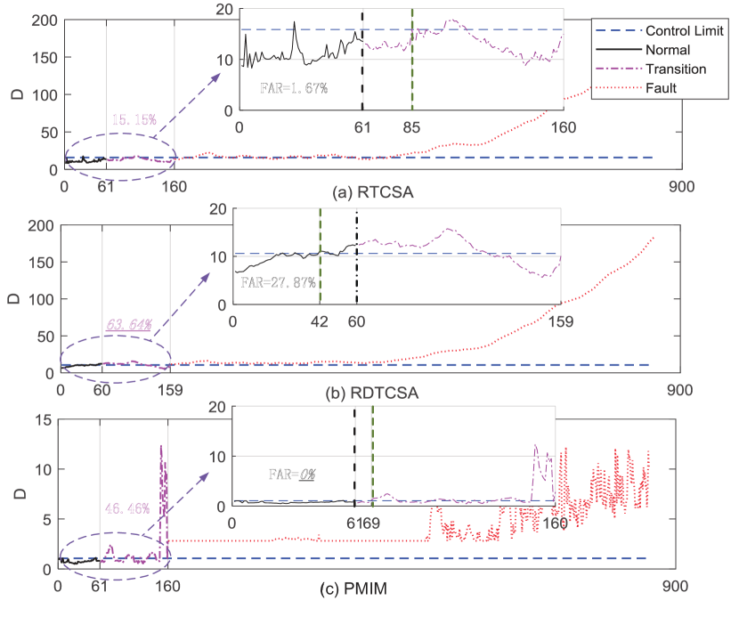
Figure 14: Detection performances of TCSA methods for fault 21 in TEP. The occurrence of fault corresponded to the $61$-$th$ (RTCSA, PMIM) / $60$-$th$ (RDTCSA) measurements, marked by black line. The FDR values in transition phase are marked by pink. The green line indicates the first sample that detected as a fault instant.

To describe the effectiveness of our proposed PMIM by a more general data, we use the benchmark data of base model that can be downloaded from: http://web.mit.edu/braatzgroup/links.html. $960$ samples are used as test data. The fault is induced after $8$ hours, which corresponds to the $161$-th samples. Because the length of sliding window is $100$, the fault occurs at the time index $61$ (for RTCSA and PMIM) and $60$ (for RDTCSA). Take fault $21$ as an example, the detection performances of RTCSA, RDTCSA and our PMIM are shown in Fig. 14. The FARs of three competing methods are $1.67\%$ (for RTCSA), $27.87\%$ (for RDTCSA) and $0$ (for PMIM). Obviously, our method has the lowest FAR in this example. RTCSA detects a fault at the $85$-th sample, which suggests a detection delay of $24$ samples. By contrast, our PMIM detects a fault at time index $69$, with a detection delay of only $8$ samples. RDTCSA fails in this example, because it alarms a fault at time index $42$ ($18$ samples ahead of the occurrence of fault), which is a false detection.

6 Conclusion

This work presents a new information-theoretic method on fault detection. Before our work, most of the information-theoretic fault detection methods just use mutual information (MI) as a dependence measure to select the most informative dimensions to circumvent the curse of dimensionality. Distinct from these efforts, our method does not perform feature selection. Instead, we constructed a MI matrix to quantify all nonlinear dependencies between pairwise dimensions of data. We introduced the matrix-based Rényi’s $\alpha$-order mutual information estimator to estimate the MI value in each entry of the MI matrix. The new estimator avoids the density estimation and is well-suited for complex industrial process. By monitoring different orders of statistics associated with the transformed components of the MI matrix, we demonstrated that our method is able to quickly detect the distributional change of the underlying process, and to identify the root variables that cause the fault. We compared our method with four state-of-the-art fault detection methods on both synthetic data and the real-world Tennessee Eastman process. Empirical results suggest that our method improves the fault detection rate (FDR) and significantly reduces the false alarm rate (FAR). We also presented a thorough analysis on effects of hyper-parameters (e.g., window length $w$ and kernel width $\sigma$) to the performance of our method and illuminated how they control the trade-off between FAR and FDR.

Finally, one should note that the MI matrix is a powerful tool to analyze and discover pairwise interactions in high dimensions of multivariate time series in signal processing, economics and other scientific disciplines. Unfortunately, most of its properties, characteristics, and practical advantages are still largely unknown. This work is a first step to understand the value of non-parametric dependence measures (especially the MI matrix) in monitoring industrial process. We will continue working along this direction to improve the performance of our method and also theoretically explore its fundamental properties.

Appendix A

For reproducible results, we provide key functions (in MATLTB $2019$a) of the proposed PMIM. Specifically, “mutual_information_estimation.m” estimates the matrix-based Rényi’s $\alpha$-order mutual information (Eq. 6), in which the “gaussianMatrix.m” evaluates the kernel induced Gram matrix (Eq. 18). “MI_matrix.m” obtains a series of mutual information matrix at each time instant $k$. “MITCSA.m” computes the similarity index (Eq. 14).

⬇

1function mutual_information = mutual_information_estimation(variable1,variable2,sigma,alpha)

2% variable 1 is i-th dimensional of the process measurement (i-th variable)

3% variable 2 is j-th dimensional of the process measurement (j-th variable)

4%% estimate entropy for variable 1

5K_x = real(guassianMatrix(variable1,sigma))/size(variable1,1);

6[~, L_x] = eig(K_x);

7lambda_x = abs(diag(L_x));

8H_x = (1/(1-alpha))*log((sum(lambda_x.^alpha)));

9

10%% estimate entropy for variable 2

11K_y = real(guassianMatrix(variable2,sigma))/size(variable2,1);

12[~, L_y] = eig(K_y);

13lambda_y = abs(diag(L_y));

14H_y = (1/(1-alpha))*log((sum(lambda_y.^alpha)));

15

16%% estimate joint entropy H(X,Y)

17K_xy = K_x.*K_y.*size(variable1,1);

18[~,L_xy] = eig(K_xy);

19lambda_xy = abs(diag(L_xy));

20H_xy = (1/(1-alpha))*log( (sum(lambda_xy.^alpha)));

21

22%% estimate mutual information I(X;Y)

23mutual_information = H_x + H_y - H_xy;

24

25end

⬇

1function K = guassianMatrix(X,sigma)

2G = X*X’;

3K = bsxfun(@minus, 2*G, diag(G)’);

4K = exp((1/(2*sigma^2))*bsxfun(@minus, K, diag(G)));

5

6end

⬇

1function MImatrixcell = MI_matrix(data,sigma,alpha,MIsize)

2% Input:

3% data is the sample matrix X

4% MIsize is the length of sliding window

5% alpha is the entropy order

6% sigma is the kernel size

7% Output:

8% MImatrixcell is a series of mutual information(MI) matrix over the whole process

9[nums nums_vars]=size(data);

10[Data, av, st]=zscore(data);

11for k=1:nums-MIsize+1

12 dydata=Data(k:k+MIsize-1,:);

13% MImatrix is the MI matrix at time instant k

14 for i=1:nums_vars

15 for j=i:nums_vars

16 MImatrix(i,j) = mutual_information_estimation(dydata(:,i),dydata(:,j),sigma,alpha);

17 MImatrix(j,i) = MImatrix(i,j);

18 end

19 end

20 MImatrixcell{1,k} = MImatrix;

21end

22

23end

⬇

1function Di = MITCSA(data,MImatrixcell,MIsize)

2% Input:

3% data is the sample matrix X

4% MIdata is the MI matrix of data

5% MIsize is the length w of sliding window

6% Output:

7% Di is the similarity index

8for i=1:length(MImatrixcell)

9 MImatrix=MImatrixcell{1,i};

10% Eigen-decomposition of the mutual information(MI) matrix

11 [Vet C]=eig(MImatrix,’vector’);

12% The MI based transform components(TCs)

13 T=data{1,i}*Vet;

14% The statistic of TCs

15 Mu(i,:) = mean(T);% mean

16 V(i,:) = sum((T-Mu(i,:)).^2)/MIsize; % variance

17 S1(i,:)= sum((T-Mu(i,:)).^3)/MIsize;

18 K1(i,:)= sum((T-Mu(i,:)).^4)/MIsize;

19 S(i,:) = S1(i,:)./(V(i,:).^(3/2)); % skewness

20 K(i,:) = K1(i,:)./(V(i,:).^2)-3; % kurtosis

21end

22Oo = [Mu,V,S,K];

23Mu_mu = mean(Mu);% the reference mean

24Oo_mu = mean(Oo);

25Oo_sv = std(Oo,1);

26% The calculation of the similarity index

27for i=1:length(MImatrixcell)

28 D1 = Oo(i,:)-Oo_mu;

29 D = D1./(Oo_sv);

30 Di(1,i) = norm(D,inf);

31end

32

33end

Appendix B

Tennessee Eastman process (TEP) created by the Eastman Chemical Company is designed to provide an actual industrial process for evaluating process control strategies[60, 61]. It is composed of five major unit operations including a chemical reactor, a product condenser, a recycle compressor, a vapor-liquid separator and a product stripper. Fig. 15 shows its schematic. 21 types of identified faults are listed in Table 5. In this work, $33$ different variables ($22$ process measurements and $11$ manipulated measurements) constitute the input of PMIM, as listed in Table 6. In this sense, the MI matrix in TEP is of size $33\times 33$.

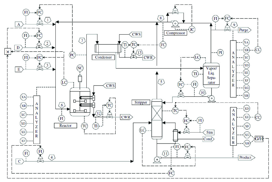
Figure 15: The schematic of TEP.

Table 5: Descriptions of process faults in TEP

No.	Description	Type
1	A/C feed ratio, B composition constant (Stream 4)	Step
2	B composition, A/C ratio constant (Stream 4)	Step
3	D feed temperature (Stream 2)	Step
4	Reactor cooling water inlet temperature	Step
5	Condenser cooling water inlet temperature	Step
6	A feed loss (Stream 1)	Step
7	C header pressure loss- reduced availability (Stream 4)	Step
8	A, B, C feed composition (Stream 4)	Random variation
9	D feed temperature (Stream 2)	Random variation
10	C feed temperature (Stream 4)	Random variation
11	Reactor cooling water inlet temperature	Random variation
12	Condenser cooling water inlet temperature	Random variation
13	Reaction kinetics slow	Slow drift
14	Reactor cooling water valve	Sticking
15	Condenser cooling water valve	Sticking
16	Unknown (deviations of heat transfer within stripper (heat exchanger))	Unknown
17	Unknown (deviations of heat transfer within reactor)	Unknown
18	Unknown (deviations of heat transfer within condenser)	Unknown
19	Unknown	Unknown
20	Unknown	Unknown
21	The valve for Stream 4 was fixed at the steady state position	Constant position

Table 6: Monitoring variables in TEP

No.	Manipulated measurements	No.	Continuous measurements
1	D feed flow valve (stream 2)	6	Reactor feed rate (stream 6)
2	E feed flow valve (stream 3)	7	Reactor pressure
3	A feed flow valve (stream 1)	8	Reactor level
4	total feed flow valve (stream 4)	9	Reactor temperature
5	compressor recycle valve	10	Purge rate (stream 9)
6	purge valve (stream 9)	11	Product separator temperature
7	separator pot liquid flow valve (stream 10)	12	Product separator level
8	stripper liquid product flow valve (stream 11)	13	Product separator pressure
9	stripper steam valve	14	Product separator underflow
10	reactor cooling water flow	15	Stripper level
11	condenser cooling water flow	16	Stripper pressure
Sampling interval: 6 mins		17	Stripper underflow
No.	Continuous measurements	18	Stripper temperature
1	A feed (stream 1)	19	Stripper steam flow
2	D feed (stream 2)	20	Compressor work
3	E feed (stream 3)	21	Reactor cooling water outlet temperature
4	A and C feed (stream 4)	22	Separator cooling water outlet temperature
5	Recycle flow (stream 4)	Sampling interval: 3 mins

References

- [1] S. Yin, S. X. Ding, X. Xie, et al, A review on basic data-driven approaches for industrial process monitoring, IEEE Transactions on Industrial Electronics 61 (11) (2014) 6418–6428.
- [2] S. Yin, H. Gao, O. Kaynak, Data-driven control and process monitoring for industrial applications, part i, IEEE Transactions on Industrial Electronics 61 (11) (2014) 6356–6359.
- [3] J. F. Macgregor, T. Kourti, Statistical process control of multivariate processes, Control Engineering Practice 3 (4) (1995) 403–414.
- [4] R. L. Mason, J. C. Young, Multivariate statistical process control with industrial applications, Technometrics 46 (4) (2002) 484–485.
- [5] Y. Wang, Y. Si, B. Huang, et al, Survey on the theoretical research and engineering applications of multivariate statistics process monitoring algorithms: 2008-2017, The Canadian Journal of Chemical Engineering 96 (10) (2018) 2073–2085.
- [6] B. M. Wise, L. RickerN, D. F. Veltkamp, B. R. Kowalski, A theoretical basis for the use of principal component models for monitoring multivariate process, Process Control and Quality 1 (1) (1990) 41–51.
- [7] J. V. Kresta, J. F. Macgregor, T. E. Marlin, Multivariate statistical monitoring of process operating performance, The Canadian Journal of Chemical Engineering 69 (1) (1991) 35–47.
- [8] J. M. Lee, C. K. Yoo, I. B. Lee, Statistical process monitoring with independent component analysis, Journal of Process Control 14 (5) (2004) 467–485.
- [9] S. J. Qin, Statistical process monitoring: basics and beyond, Journal of Chemometrics 17 (2003) 480–502.
- [10] H. Hotelling, Relations between two sets of variates, Biometrika 28 (3/4) (1936) 321–377.
- [11] W. Ku, R. H. Storer, C. Georgakis, Disturbance detection and isolation by dynamic principal component analysis, Chemometrics and Intelligent Laboratory Systems 30 (1995) 179–196.
- [12] Y. N. Dong, S. J. Qin, A novel dynamic pca algorithm for dynamic data modeling and process monitoring, Journal of Process Control 67 (2018) 1–11.
- [13] C. Tong, T. Lan, X. Shi, Double-layer ensemble monitoring of non-gaussian processes using modified independent component analysis, ISA transactions 68 (2017) 181–188.
- [14] Y. W. Zhang, Y. Zhang, Fault detection of non-gaussian processes based on modified independent component analysis, Chemical Engineering Science 65 (16) (2010) 4630–4639.
- [15] C. D. Tong, T. Lan, X. H. Shi, Ensemble modified independent component analysis for enhanced non-gaussian process monitoring, Control Engineering Practice 58 (2017) 34–41.
- [16] C. Alcala, S. J. Qin, Reconstruction-based contribution for process monitoring, Automatica 45 (7) (2009) 1593–1600.
- [17] L. Zhang, J. Lin, R. Karim, Sliding window-based fault detection from high-dimensional data streams, IEEE Transactions on Systems, Man, and Cybernetics: Systems 47 (2) (2016) 289–303.
- [18] Z. W. Chen, S. Ding, T. Peng, C. H. Yang, Fault detection for non-gaussian processes using generalized canonical correlation analysis and randomized algorithms, IEEE Transactions on Industrial Electronics 65 (2) (2017) 1559–1567.
- [19] Q. Jiang, S. Ding, Y. Wang, X. F. Yan, Data-driven distributed local fault detection for large-scale processes based on the ga-regularized canonical correlation analysis, IEEE Transactions on Industrial Electronics 64 (10) (2017) 8148–8157.
- [20] J. Wang, Q. P. He, Multivariate statistical process monitoring based on statistics pattern analysis, Industrial & Engineering Chemistry Research 49 (17) (2010) 7858–7869.
- [21] S. M. Zhang, C. H. Zhao, Hybrid independent component analysis (h-ica) with simultaneous analysis of high-order and second-order statistics for industrial process monitoring, Chemometrics and Intelligent Laboratory Systems 185 (2019) 47–58.
- [22] M. S. Choudhury, S. L. Shah, N. F. Thornhill, Diagnosis of poor control-loop performance using higher-order statistics, Automatica 40 (2004) 1719–1728.
- [23] Q. P. He, J. Wang, Statistics pattern analysis: A new process monitoring framework and its application to semiconductor batch processes, AIChE Journal 57 (1) (2011) 107–121.
- [24] J. Shang, M. Chen, H. Ji, et al, Recursive transformed component statistical analysis for incipient fault detection, Automatica 80 (2017) 313–327.
- [25] J. Shang, M. Chen, Recursive dynamic transformed component statistical analysis for fault detection in dynamic processes, IEEE Transactions on Industrial Electronics 65 (1) (2018) 578–588.
- [26] B. Q. Zhou, X. S. Gu, Multi-block statistics local kernel principal component analysis algorithm and its application in nonlinear process fault detection, Neurocomputing 376 (2020) 222–231.
- [27] G. Jia, Y. Wang, B. Huang, Dynamic higher-order cumulants analysis for state monitoring based on a novel lag selection, Inform Science 331 (2016) 45–66.
- [28] F. Lv, C. Wen, M. Liu, Representation learning based adaptive multimode process monitoring, Chemometrics and Intelligent Laboratory Systems 181 (2018) 95–104.
- [29] C. H. Chang, Deep and shallow architecture of multilayer neural networks, IEEE Transactions on Neural Networks and Learning Systems 26 (10) (2015) 2477–2486.
- [30] G. H. Bazan, P. R. Scalassara, W. Endo, et al, Stator fault analysis of three-phase induction motors using information measures and artificial neural networks, Electric Power Systems Research 143 (2017) 347–356.
- [31] X. Zhao, P. Shang, J. Huang, Mutual-information matrix analysis for nonlinear interactions of multivariate time series, Nonlinear Dynamics 588 (2017) 477–487.
- [32] S. Verron, T. Tiplica, A. Kobi, Fault detection and identification with a new feature selection based on mutual information, Journal of Process Control 18 (5) (2008) 479–490.
- [33] M. Jiang, M. A. Munawar, T. Reidemeister, et al, Efficient fault detection and diagnosis in complex software systems with information-theoretic monitoring, IEEE Transactions on Dependable and Secure Computing 8 (4) (2011) 510–522.
- [34] M. M. Rashid, J. Yu, A new dissimilarity method integrating multidimensional mutual information and independent component analysis for non-gaussian dynamic process monitoring, Chemometrics and Intelligent Laboratory Systems 115 (2012) 44–58.
- [35] J. Yu, J. Chen, M. M. Rashid, Multiway independent component analysis mixture model and mutual information based fault detection and diagnosis approach of multiphase batch processes, AIChE Journal 59 (8) (2013) 2761–2779.
- [36] B. Jiang, W. Sun, R. D. Braatz, An information-theoretic framework for fault detection evaluation and design of optimal dimensionality reduction methods, IFAC 51 (24) (2018) 1311–1316.
- [37] A. Joshi, P. Deignan, P. Meckl, et al, Information theoretic fault detection, Proceedings of the 2005, American Control Conference (2005) 1642–1647.
- [38] C. E. Shannon, A mathematical theory of communication, Bell system technical journal 27 (3) (1948) 379–423.
- [39] T. M. Cover, J. A. Thomas, Elements of information theory, John Wiley & Sons, New York, 1991.
- [40] P. E. Latham, Y. Roudi, Mutual information, Scholarpedia 4 (2009) 1658.
- [41] S. K. Jakobsen, Mutual information matrices are not always positive semidefinite, IEEE Transactions on Information Theory 60 (5) (2014) 2694–2696.
- [42] J. C. Principe, Information theoretic learning: Rényi’s entropy and kernel perspectives, Springer Science & Business Media, 2010.
- [43] T. Cover, J. Thomas, J. Wiley, Elements of Information Theory, Tsinghua University Press, 2003.
- [44] M. Muller-Lennert, F. Dupuis, O. Szehr, S. Fehr, M. Tomamichel, On quantum rényi’s entropies: A new generalization and some properties, Journal of Mathematical Physics 54 (12) (2013).
- [45] P. Bromiley, N. Thacker, E. Bouhova-Thacker, Shannon entropy, rényi’s entropy, and information, Statistics and Inf. Series (2004-004) (2004).
- [46] S. Yu, L. G. S. Giraldo, R. Jenssen, J. C. Principe, Multivariate extension of matrix-based rényi’s -order entropy functional, IEEE Transactions on Pattern Analysis and Machine Intelligence (2019).
- [47] B. C. Ross, Mutual information between discrete and continuous data sets, PloS one 9 (2) (2014) e87357.
- [48] W. Gao, S. Kannan, S. Oh, P. Viswanath, Estimating mutual information for discrete-continuous mixtures, in: Advances in neural information processing systems, 2017, pp. 5986–5997.
- [49] L. G. S. Giraldo, M. Rao, J. C. Principe, Measures of entropy from data using infinitely divisible kernels, IEEE Transactions on Information Theory 61 (1) (2015) 535–548.
- [50] R. Bhatia, Infinitely divisible matrices, American Mathematical Monthly 113 (3) (2006) 221–C235.
- [51] J. M. Lee, S. J. Qin, I. B. Lee, Fault detection and diagnosis based on modified independent component analysis, AIChE Journal 52 (2006) 3501–3514.
- [52] R. A. Ince, B. L. Giordano, C. Kayser, G. A. Rousselet, J. Gross, P. G. Schyns, A statistical framework for neuroimaging data analysis based on mutual information estimated via a gaussian copula, Human brain mapping 38 (3) (2017) 1541–1573.
- [53] F. J. Dyson, Statistical theory of the energy levels of complex systems i, Journal of Mathematical Physics 3 (1) (1962) 140–156.
- [54] S. X. Ding, Model-Based Fault Diagnosis Techniques—Design Schemes, Algorithms and Tools (2nd ed.), Springer-Verlag, 2013.
- [55] Z. W. Chen, K. Zhang, Y. A. Shardt, S. X. Ding, et al, Comparison of two basic statistics for fault detection and process monitoring, IFAC-Papers On Line 50 (1) (2017) 14776–14781.
- [56] B. Ratner, The correlation coefficient: Its values range between +1/-1, or do they?, Journal of targeting, measurement and analysis for marketing 17 (2) (2009) 139–142.
- [57] S. Yu, J. C. Principe, Simple stopping criteria for information theoretic feature selection, Entropy 21 (1) (2019) 99.
- [58] B. W. Silverman, Density estimation for statistics and data analysis, CRC press 26 (1986).
- [59] J. Shi, J. Malik, Normalized cuts and image segmentation, IEEE Transactions on pattern analysis and machine intelligence 22 (8) (2000) 888–905.
- [60] J. Downs, F. Vogel, A plant-wide industrial process control problem, Computers and chemical engineering 17 (3) (1993) 245–255.
- [61] N. L. Ricker, Optimal steady-state operation of the tennessee eastman challenge process, Computers and chemical engineering 19 (9) (1995) 949–959.
- [62] L. H. Chiang, R. D. Braatz, E. L. Russell, Fault detection and diagnosis in industrial systems, Springer, 2001.
- [63] E. L. Russell, L. H. Chiang, R. D. Braatz, Data-driven methods for fault detection and diagnosis in chemical processes, Springer, 2012.
- [64] Z. Chen, H. Fang, Y. Chang, Weighted data-driven fault detection and isolation: a subspace-based approach and algorithms, IEEE Transactions on Industrial Electronics 63 (5) (2016) 3290–3298.
- [65] G. Li, C. F. Alcala, S. J. Qin, D. Zhou, Generalized reconstruction-based contributions for output-relevant fault diagnosis with application to the tennessee eastman process, IEEE transactions on control systems technology 19 (5) (2010) 1114–1127.