1.5pt

Technical details of distributed localization

1. Proof of Theorem $1$

For any three different nodes $p_{i},p_{j},p_{k}$ in $\mathbb{R}^{3}$, the condition $\theta_{i}+\theta_{j}+\theta_{k}=\pi$ must hold. The angle constraints can be rewritten as

$$w_{ik}d_{ik}d_{ij}\cos\theta_{i}+w_{ki}d_{ik}d_{jk}\cos\theta_{k}=0,$$ (1)

$$w_{ij}d_{ik}d_{ij}\cos\theta_{i}+w_{ji}d_{ij}d_{jk}\cos\theta_{j}=0,$$ (2)

$$w_{jk}d_{jk}d_{ij}\cos\theta_{j}+w_{kj}d_{ik}d_{jk}\cos\theta_{k}=0,$$ (3)

with $w_{ik}^{2}+w_{ki}^{2}\neq 0$, $w_{ij}^{2}+w_{ji}^{2}\neq 0$, and $w_{jk}^{2}+w_{kj}^{2}\neq 0$.

First, we introduce Lemma 7 and Lemma 8 below for proving Theorem 1.

Lemma 7. $p_{i},p_{j},p_{k}$ are non-colinear if the parameters in (1)-(3) satisfy $w_{ik}w_{ij}w_{jk}w_{ki}w_{ji}w_{kj}=0$.

Proof.

When $w_{ik}w_{ij}w_{jk}w_{ki}w_{ji}w_{kj}=0$, without loss of generality, suppose $w_{ik}=0$, since $w_{ik}^{2}+w_{ki}^{2}\neq 0$, we have $\theta_{k}=\frac{\pi}{2}$, $\theta_{i}+\theta_{j}=\frac{\pi}{2}$ from (1). Hence, $p_{i},p_{j},p_{k}$ are non-colinear. Similarly, we can prove that $p_{i},p_{j},p_{k}$ are non-colinear if the parameter $w_{ij}=0$, or $w_{jk}=0$, or $w_{ki}=0$, or $w_{ji}=0$, or $w_{kj}=0$. ∎

If $w_{ik}w_{ij}w_{jk}w_{ki}w_{ji}w_{kj}\neq 0$, (1)-(3) can be rewritten as

$$\frac{\cos\theta_{i}}{\cos\theta_{k}}=-\frac{w_{ki}d_{jk}}{w_{ik}d_{ij}},$$ (4)

$$\frac{\cos\theta_{i}}{\cos\theta_{j}}=-\frac{w_{ji}d_{jk}}{w_{ij}d_{ik}},$$ (5)

$$\frac{\cos\theta_{j}}{\cos\theta_{k}}=-\frac{w_{kj}d_{ik}}{w_{jk}d_{ij}}.$$ (6)

From (4) and (5), we have

$$d_{ij}=-\frac{\cos\theta_{k}}{\cos\theta_{i}}\frac{w_{ki}}{w_{ik}}d_{jk},$$ (7)

$$d_{ik}=-\frac{\cos\theta_{j}}{\cos\theta_{i}}\frac{w_{ji}}{w_{ij}}d_{jk}.$$ (8)

Note that $\cos\theta_{i}=\frac{d_{ij}^{2}+d_{ik}^{2}-d_{jk}^{2}}{2d_{ij}d_{ik}}$, $\cos\theta_{j}=\frac{d_{ij}^{2}+d_{jk}^{2}-d_{ik}^{2}}{2d_{ij}d_{jk}}$, $\cos\theta_{k}=\frac{d_{ik}^{2}+d_{jk}^{2}-d_{ij}^{2}}{2d_{ik}d_{jk}}$. Combining (7) and (8), it yields

$$\frac{d_{ij}^{2}+d_{ik}^{2}-d_{jk}^{2}}{d_{ik}^{2}+d_{jk}^{2}-d_{ij}^{2}}+\frac{d_{ij}^{2}+d_{ik}^{2}-d_{jk}^{2}}{d_{ij}^{2}+d_{jk}^{2}-d_{ik}^{2}}=-(\frac{w_{ki}}{w_{ik}}+\frac{w_{ji}}{w_{ij}}).$$ (9)

Lemma 8. When the parameters in (1)-(3) satisfy $w_{ik}w_{ij}w_{jk}w_{ki}w_{ji}w_{kj}\neq 0$, $p_{i},p_{j},p_{k}$ are colinear if and only if

$$\frac{w_{ki}}{w_{ik}}+\frac{w_{ji}}{w_{ij}}=1,\text{or}\ \frac{w_{ij}}{w_{ji}}+\frac{w_{kj}}{w_{jk}}=1,\text{or}\ \frac{w_{ik}}{w_{ki}}+\frac{w_{jk}}{w_{kj}}=1.$$ (10)

Proof.

(Necessity) If $p_{i},p_{j},p_{k}$ are colinear, there are three cases: (i) $\theta_{i}=\pi$, $\theta_{j},\theta_{k}=0$; (ii) $\theta_{j}=\pi$, $\theta_{i},\theta_{k}=0$; (iii) $\theta_{k}=\pi$, $\theta_{i},\theta_{j}=0$. For the case (i) that $\theta_{i}=\pi$, $\theta_{j},\theta_{k}=0$, we have $d_{ij}+d_{ik}=d_{jk}$. Substituting $d_{ij}+d_{ik}=d_{jk}$ into (9), we get

$$\frac{w_{ki}}{w_{ik}}+\frac{w_{ji}}{w_{ij}}=1.$$ (11)

Similarly, the conditions can be derived for the other two cases (ii)-(iii).

(Sufficiency) If $\frac{w_{ki}}{w_{ik}}+\frac{w_{ji}}{w_{ij}}=1$, (9) becomes

$$\frac{d_{ij}^{2}+d_{ik}^{2}-d_{jk}^{2}}{d_{ik}^{2}+d_{jk}^{2}-d_{ij}^{2}}+\frac{d_{ij}^{2}+d_{ik}^{2}-d_{jk}^{2}}{d_{ij}^{2}+d_{jk}^{2}-d_{ik}^{2}}=-1.$$ (12)

Then, (12) can be rewritten as

$$(d_{ij}^{2}+d_{ik}^{2}-d_{jk}^{2})^{2}=4d_{ik}^{2}d_{ij}^{2}.$$ (13)

Since $\cos\theta_{i}=\frac{d_{ij}^{2}+d_{ik}^{2}-d_{jk}^{2}}{2d_{ij}d_{ik}}$, (13) becomes

$$4d_{ij}^{2}d_{ik}^{2}\cos^{2}\theta_{i}=4d_{ij}^{2}d_{ik}^{2},\rightarrow\cos^{2}\theta_{i}=1.$$ (14)

Hence, $\theta_{i}=0$ or $\pi$, i.e., $p_{i},p_{j},p_{k}$ must be colinear. Similarly, we can prove that $p_{i},p_{j},p_{k}$ must be colinear for the other two cases $\frac{w_{ij}}{w_{ji}}+\frac{w_{kj}}{w_{jk}}=1\ \text{and}\ \frac{w_{ik}}{w_{ki}}+\frac{w_{jk}}{w_{kj}}=1$. ∎

Next, we will prove that the angles $\theta_{i},\theta_{j},\theta_{k}\in[0,\pi]$ are determined uniquely by the parameters $w_{ik},w_{ki},w_{ij},w_{ji},$ $w_{jk},w_{kj}$ in (1)-(3). From Lemma 7 and Lemma 8, we can know that there are only three cases for (1)-(3):

1. $w_{ik}w_{ij}w_{jk}w_{ki}w_{ji}w_{kj}=0$;

2. $w_{ik}w_{ij}w_{jk}w_{ki}w_{ji}w_{kj}\neq 0$, and $\frac{w_{ki}}{w_{ik}}+\frac{w_{ji}}{w_{ij}}=1$, or  $\frac{w_{ij}}{w_{ji}}+\frac{w_{kj}}{w_{jk}}=1$, or  $\frac{w_{ik}}{w_{ki}}+\frac{w_{jk}}{w_{kj}}=1$;

3. $w_{ik}w_{ij}w_{jk}w_{ki}w_{ji}w_{kj}\neq 0$, and $\frac{w_{ki}}{w_{ik}}+\frac{w_{ji}}{w_{ij}},\frac{w_{ij}}{w_{ji}}+\frac{w_{kj}}{w_{jk}},\frac{w_{ik}}{w_{ki}}+\frac{w_{jk}}{w_{kj}}\neq 1$.

The above three cases $(\text{i})\!-\!(\text{iii})$ are analyzed below.

For the case $(\text{i})$, from Lemma 7, we can know that $p_{i},p_{j},p_{k}$ are non-colinear and form a triangle $\bigtriangleup_{ijk}(p)$. Without loss of generality, suppose $w_{ik}=0$, since $w_{ik}^{2}+w_{ki}^{2}\neq 0$, we have $\theta_{k}=\frac{\pi}{2}$, $\theta_{i}+\theta_{j}=\frac{\pi}{2}$ from (1). Since $\theta_{i}+\theta_{j}=\frac{\pi}{2}$, we have $w_{ij}\cdot w_{ji}<0$ from (5). According to the sine rule, $\frac{d_{jk}}{d_{ik}}=\frac{\sin\theta_{i}}{\sin\theta_{j}}$. Then, (5) becomes

$$\frac{\tan\theta_{i}}{\tan\theta_{j}}=-\frac{w_{ij}}{w_{ji}}.$$ (15)

Since $\theta_{j}=\frac{\pi}{2}-\theta_{i}$, from (15), we have

$$\tan\theta_{i}=\sqrt{-\frac{w_{ij}}{w_{ji}}},\rightarrow\theta_{i}=\arctan\sqrt{-\frac{w_{ij}}{w_{ji}}}.$$ (16)

Similarly, we can prove that $\theta_{i},\theta_{j},\theta_{k}$ can be determined uniquely if the parameter $w_{ij},w_{jk},w_{ki},w_{ji},$ or $w_{kj}$ equals $0$.

For the case $(\text{ii})$, from Lemma 8, we can know that $p_{i},p_{j},p_{k}$ are colinear. Two of $\theta_{i},\theta_{j},\theta_{k}$ must be $0$. If $w_{kj}w_{jk}<0$, i.e., $\frac{\cos\theta_{j}}{\cos\theta_{k}}>0$ from (6), we have $\theta_{i}=\pi$, $\theta_{j},\theta_{k}=0$. Similarly, we have $\theta_{j}=\pi$, $\theta_{i},\theta_{k}=0$ if $w_{ki}w_{ik}<0$, and $\theta_{k}=\pi$, $\theta_{i},\theta_{j}=0$ if $w_{ji}w_{ij}<0$.

For the case $(\text{iii})$, from Lemma 8, we can know that $p_{i},p_{j},p_{k}$ are non-colinear and form a triangle $\bigtriangleup_{ijk}(p)$. For this triangle $\bigtriangleup_{ijk}(p)$, at most one of $\theta_{i},\theta_{j},\theta_{k}$ is an obtuse angle. Hence, there are only four possible cases: $(\text{a})$ $w_{ki}w_{ik},w_{ji}w_{ij},w_{kj}w_{jk}<0$; $(\text{b})$ $w_{ki}w_{ik},w_{ji}w_{ij}>0,w_{kj}w_{jk}<0$; $(\text{c})$ $w_{ki}w_{ik},w_{kj}w_{jk}>0,w_{ji}w_{ij}<0$; $(\text{d})$ $w_{ji}w_{ij},w_{kj}w_{jk}>0,w_{ki}w_{ik}<0$. For the case $(\text{a})$, we have $\theta_{i},\theta_{j},\theta_{k}<\frac{\pi}{2}$. From (4) and (5), we have

$$\tan\theta_{k}=-\frac{w_{ki}}{w_{ik}}\tan\theta_{i},\ \ \tan\theta_{j}=-\frac{w_{ji}}{w_{ij}}\tan\theta_{i}.$$ (17)

Note that $\tan\theta_{i}=\tan(\pi-\theta_{j}-\theta_{k})=\frac{\tan\theta_{j}+\tan\theta_{k}}{\tan\theta_{j}\tan\theta_{k}-1}$. Based on (17), we have

$$\tan\theta_{i}=\sqrt{\frac{1-\frac{w_{ki}}{w_{ik}}-\frac{w_{ji}}{w_{ij}}}{\frac{w_{ki}w_{ji}}{w_{ik}w_{ij}}}}.$$ (18)

Then, we can obtain the angle $\theta_{i}$ by

$$\theta_{i}=\arctan\sqrt{\frac{1-\frac{w_{ki}}{w_{ik}}-\frac{w_{ji}}{w_{ij}}}{\frac{w_{ki}w_{ji}}{w_{ik}w_{ij}}}}.$$ (19)

Similarly, the angles $\theta_{j}$ and $\theta_{k}$ can also be obtained. Using this way, we can prove that $\theta_{i},\theta_{j},\theta_{k}$ can be determined uniquely by the parameters $w_{ik},w_{ki},w_{ij},w_{ji},w_{jk},w_{kj}$ for the cases $(\text{b})$-$(\text{d})$.

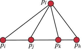
Figure 1: 3-D local-relative-bearing-based network.

2. Proof of Lemma $2$

Proof.

Since $\mu_{ij}e_{ij}\!+\!\mu_{ik}e_{ik}\!+\!\mu_{ih}e_{ih}\!+\!\mu_{il}e_{il}=\mathbf{0}$ and $w_{ik}e_{ik}^{T}e_{ij}+w_{ki}e_{ki}^{T}e_{kj}=0$, for the scaling space $S_{s}$, it is straightforward that $\eta_{d}^{T}p=\mathbf{0}$ and $\eta_{r}^{T}p=0$. For the translation space $S_{t}$, we have $\eta_{d}^{T}(\mathbf{1}_{n}\otimes{I}_{3})=\mathbf{0}$ and $\eta_{r}^{T}(\mathbf{1}_{n}\otimes{I}_{3})=\mathbf{0}$. For the rotation space $S_{r}=\{(I_{n}\otimes A)p,A+A^{T}=\mathbf{0},A\in\mathbb{R}^{3\times 3}\}$, it follows that $\eta_{d}^{T}(I_{n}\otimes A)p=A(\mu_{ij}e_{ij}\!+\!\mu_{ik}e_{ik}\!+\!\mu_{ih}e_{ih}\!+\!\mu_{il}e_{il})=\mathbf{0}$ and

$$\begin{array}[]{ll}\eta_{r}^{T}(I_{n}\otimes A)p\\ =w_{ik}p_{i}^{T}(A+A^{T})p_{i}\!+\!(w_{ki}\!-\!w_{ik})p_{j}^{T}(A\!+\!A^{T})p_{i}\\ -(w_{ik}\!+\!w_{ki})p_{k}^{T}(A\!+\!A^{T})p_{i}+(w_{ik}\!-\!w_{ki})p_{k}^{T}(A\!+\!A^{T})p_{j}\\ +w_{ki}p_{k}^{T}(A\!+\!A^{T})p_{k}=0.\end{array}$$ (20)

Then, the conclusion follows. ∎

3. Local-relative-bearing-based Displacement Constraint

$g_{ij}=\frac{e_{ij}}{d_{ij}}\in\mathbb{R}^{3}$ is the relative bearing of $p_{j}$ with respect to $p_{i}$ in $\Sigma_{g}$. For the node $i$ and its neighbors $j,k,h,l$ in $\mathbb{R}^{3}$, the matrix $g_{i}=(g_{ij},g_{ik},g_{ih},g_{il})\in\mathbb{R}^{3\times 4}$ is a wide matrix. From the matrix theory, there must be a non-zero vector $\bar{\mu}_{i}=(\bar{\mu}_{ij},\bar{\mu}_{ik},\bar{\mu}_{ih},\bar{\mu}_{il})^{T}\in\mathbb{R}^{4}$ such that $g_{i}\bar{\mu}_{i}=\mathbf{0}$, i.e.,

$$\bar{\mu}_{ij}g_{ij}+\bar{\mu}_{ik}g_{ik}+\bar{\mu}_{ih}g_{ih}+\bar{\mu}_{il}g_{il}=\mathbf{0},$$ (21)

where $\bar{\mu}_{ij}^{2}+\bar{\mu}_{ik}^{2}+\bar{\mu}_{ih}^{2}+\bar{\mu}_{il}^{2}\neq 0$.

The equation $g_{i}\bar{\mu}_{i}=\mathbf{0}$ is a bearing constraint, based on which a displacement constraint can be obtained shown as following. The non-zero vector $(\bar{\mu}_{ij},\bar{\mu}_{ik},\bar{\mu}_{ih},\bar{\mu}_{il})^{T}$ can be calculated with local relative bearing measurements $g_{ij}^{i},g_{ik}^{i},g_{ih}^{i},g_{il}^{i}$ by solving the following equation

$$\left[\!\begin{array}[]{c c c c}g_{ij}^{i}&g_{ik}^{i}&g_{ih}^{i}&g_{il}^{i}\\ \end{array}\right]\left[\!\begin{array}[]{c}\bar{\mu}_{ij}\\ \bar{\mu}_{ik}\\ \bar{\mu}_{ih}\\ \bar{\mu}_{il}\end{array}\right]=\mathbf{0}.$$ (22)

Note that (21) can be rewritten as

$$\bar{\mu}_{ij}\frac{e_{ij}}{d_{ij}}+\bar{\mu}_{ik}\frac{e_{ik}}{d_{ik}}+\bar{\mu}_{ih}\frac{e_{ih}}{d_{ih}}+\bar{\mu}_{il}\frac{e_{il}}{d_{il}}=\mathbf{0}.$$ (23)

Assumption 1.

No two nodes are collocated in $\mathbb{R}^{3}$. Each anchor node has at least two neighboring anchor nodes, and each free node has at least four neighboring nodes. The free node and its neighbors are non-colinear.

Under Assumption 1, without loss of generality, suppose node $l$ is not colinear with nodes $i,j,k,h$ shown in the above Fig. 1. The angles among the nodes $p_{i},p_{j},p_{k},p_{h},p_{l}$ are denoted by $\xi_{ilj}\!=\!\angle p_{i}p_{l}p_{j},\xi_{ilk}\!=\!\angle p_{i}p_{l}p_{k},\xi_{ilh}\!=\!\angle p_{i}p_{l}p_{h},\xi_{ijl}\!=\!\angle p_{i}p_{j}p_{l},\xi_{ikl}\!=\!\angle p_{i}p_{k}p_{l},\xi_{ihl}\!=\!\angle p_{i}p_{h}p_{l}$. Note that these angles can be obtained by only using the local relative bearing measurements. For example, $\xi_{ilj}=g_{li}^{T}g_{lj}={g^{l}_{li}}^{T}Q_{l}^{T}Q_{l}g_{lj}^{l}={g_{li}^{l}}^{T}g_{lj}^{l}$. According to the sine rule, $\frac{d_{il}}{d_{ij}}=\frac{\sin\xi_{ijl}}{\sin\xi_{ilj}},\frac{d_{il}}{d_{ik}}=\frac{\sin\xi_{ikl}}{\sin\xi_{ilk}},\frac{d_{ih}}{d_{il}}=\frac{\sin\xi_{ilh}}{\sin\xi_{ihl}}$. Then, based on (23), we can obtain a displacement constraint by only using the local relative bearing measurements shown as

$$\mu_{ij}e_{ij}+\mu_{ik}e_{ik}+\mu_{ih}e_{ih}+\mu_{il}e_{il}=\mathbf{0},$$ (24)

where

$$\begin{array}[]{ll}&\mu_{ij}=\bar{\mu}_{ij}\frac{\sin\xi_{ijl}}{\sin\xi_{ilj}},\ \ \mu_{ik}=\bar{\mu}_{ik}\frac{\sin\xi_{ikl}}{\sin\xi_{ilk}},\\ &\mu_{ih}=\bar{\mu}_{ih}\frac{\sin\xi_{ilh}}{\sin\xi_{ihl}},\ \ \mu_{il}=\bar{\mu}_{il}.\end{array}$$ (25)

In a local-relative-bearing-based network in $\mathbb{R}^{3}$ under Assumption 1, let $\mathcal{X}_{\mathcal{G}}=\{(i,j,k,h,l)\in\mathcal{V}^{5}:(i,j),(i,k),$ $(i,h),(i,l),(j,k),(j,h),(j,l)\in\mathcal{E},j\!<\!k\!<\!h\!<\!l\}$. Each element of $\mathcal{X}_{\mathcal{G}}$ can be used to construct a local-relative-bearing-based displacement constraint.

4. Distance-based Displacement Constraint

Since the displacement constraints are invariant to translations and rotations, a congruent network of the subnetwork consisting of the node and its neighbors has the displacement constraint. Each displacement constraint can be regarded as a subnetwork, and multi-dimensional scaling can be used to obtain displacement constraint shown in the following Algorithm 1 [1].

5. Ratio-of-distance-based Displacement Constraint

For the free node $i$ and its neighbors $j,k,h,l$, under Assumption $1$, we can obtain the ratio-of-distance matrix $M_{r}$ (26) by the ratio-of-distance measurements.

$$M_{r}=\frac{1}{d_{ij}^{2}}\left[\!\begin{array}[]{c c c c c}0&d_{ij}^{2}&d_{ik}^{2}&d_{ih}^{2}&d_{il}^{2}\\ d_{ji}^{2}&0&d_{jk}^{2}&d_{jh}^{2}&d_{jl}^{2}\\ d_{ki}^{2}&d_{kj}^{2}&0&d_{kh}^{2}&d_{kl}^{2}\\ d_{hi}^{2}&d_{hj}^{2}&d_{hk}^{2}&0&d_{hl}^{2}\\ d_{li}^{2}&d_{lj}^{2}&d_{lk}^{2}&d_{lh}^{2}&0\end{array}\right].$$ (26)

Note that the displacement constraints are not only invariant to translations and rotations, but also to scalings. Hence, a network with ratio-of-distance measurements $\frac{1}{d_{ij}}\{d_{ij},\cdots,d_{hl},\cdots\}$ has the same displacement constraints as the network with distance measurements $\{d_{ij},\cdots,d_{hl},\cdots\}$, that is, the displacement constraint $\mu_{ij}e_{ij}+\mu_{ik}e_{ik}+\mu_{ih}e_{ih}+\mu_{il}e_{il}=\mathbf{0}$ can also be obtained by Algorithm $1$, where the distance matrix $M$ (27) is replaced by the the ratio-of-distance matrix $M_{r}$ (26).

Algorithm 1 Distance-based displacement constraint

1:Available information: Distance measurements among the nodes $p_{i},p_{j},p_{k},p_{h},p_{l}$. Denote $(\mathcal{\bar{G}},\bar{p})$ as a subnetwork with $\bar{p}=(p_{i}^{T},p_{j}^{T},p_{k}^{T},p_{h}^{T},p_{l}^{T})^{T}$.

2:Constructing a distance matrix $M\in\mathbb{R}^{5\times 5}$ shown as

$$M=\left[\!\begin{array}[]{c c c c c}0&d_{ij}^{2}&d_{ik}^{2}&d_{ih}^{2}&d_{il}^{2}\\ d_{ji}^{2}&0&d_{jk}^{2}&d_{jh}^{2}&d_{jl}^{2}\\ d_{ki}^{2}&d_{kj}^{2}&0&d_{kh}^{2}&d_{kl}^{2}\\ d_{hi}^{2}&d_{hj}^{2}&d_{hk}^{2}&0&d_{hl}^{2}\\ d_{li}^{2}&d_{lj}^{2}&d_{lk}^{2}&d_{lh}^{2}&0\end{array}\right].$$ (27)

3:Computer the centering matrix $J=I-\frac{1}{5}\mathbf{1}_{5}\mathbf{1}_{5}^{T}$;

4:Compute the matrix $X=-\frac{1}{2}JMJ$;

5:Perform singular value decomposition on $X$ as

$$X=V\Lambda V^{T},$$ (28)

where $V=(v_{1},v_{2},v_{3},v_{4},v_{5})\in\mathbb{R}^{5\times 5}$ is a unitary matrix, and $\Lambda=\text{diag}(\lambda_{1},\lambda_{2},\lambda_{3},\lambda_{4},\lambda_{5})$ is a diagonal matrix whose diagonal elements $\lambda_{1}\geq\lambda_{2}\geq\lambda_{3}\geq\lambda_{4}\geq\lambda_{5}$ are singular values. Since $\text{Rank}(X)\leq 3$, we have $\lambda_{4}=\lambda_{5}=0$. Denote by $V_{*}=(v_{1},v_{2},v_{3})$ and $\Lambda_{*}=\text{diag}(\lambda_{1},\lambda_{2},\lambda_{3})$;

6:Obtaining a congruent network $(\mathcal{\bar{G}},\bar{q})\cong(\mathcal{\bar{G}},\bar{p})$ with $\bar{q}=(q_{i}^{T},q_{j}^{T},q_{k}^{T},q_{h}^{T},q_{l}^{T})^{T}$, where $(q_{i},q_{j},q_{k},$ $q_{h},q_{l})=\Lambda_{*}^{\frac{1}{2}}V_{*}^{T}$;

7:Based on the congruent network $\bar{q}=(q_{i}^{T},q_{j}^{T},q_{k}^{T},q_{h}^{T},q_{l}^{T})^{T}$ of the subnetwork $\bar{p}=(p_{i}^{T},p_{j}^{T},p_{k}^{T},p_{h}^{T},p_{l}^{T})^{T}$, the parameters $\mu_{ij},\mu_{ik},\mu_{ih},\mu_{il}$ in $\mu_{ij}e_{ij}+\mu_{ik}e_{ik}+\mu_{ih}e_{ih}+\mu_{il}e_{il}=\mathbf{0}$ can be obtained by solving the following matrix equation

$$\left[\!\begin{array}[]{c c c c}q_{j}-q_{i}&q_{k}-q_{i}&q_{h}-q_{i}&q_{l}-q_{i}\\ \end{array}\right]\left[\!\begin{array}[]{c}\mu_{ij}\\ \mu_{ik}\\ \mu_{ih}\\ \mu_{il}\end{array}\right]=\mathbf{0}.$$ (29)

6. Angle-based Displacement Constraint

For a triangle $\bigtriangleup_{ijk}(p)$, according to the sine rule, the ratios of distance can be calculated by the angle measurements $\theta_{i},\theta_{j},\theta_{k}$ shown as

$$\frac{d_{ij}}{d_{ik}}=\frac{\sin\theta_{k}}{\sin\theta_{j}},\frac{d_{ij}}{d_{jk}}=\frac{\sin\theta_{k}}{\sin\theta_{i}}.$$ (30)

Under Assumption 1, the ratios of distance of all the edges among the nodes $i,j,k,h,l$ can be calculated by the angle measurements through the sine rule (30), i.e., the ratio-of-distance matrix $M_{r}$ (26) is available. Then, the displacement constraint $\mu_{ij}e_{ij}+\mu_{ik}e_{ik}+\mu_{ih}e_{ih}+\mu_{il}e_{il}=\mathbf{0}$ can be obtained by Algorithm $1$, where the distance matrix $M$ (27) is replaced by the the ratio-of-distance matrix $M_{r}$.

In an angle-based network in $\mathbb{R}^{3}$ under Assumption 1, let $\mathcal{X}_{\mathcal{G}}=\{(i,j,k,h,l)\in\mathcal{V}^{5}:(i,j),(i,k),$ $(i,h),(i,l),(j,k),(j,h),(j,l),(k,h),(k,l),(h,l)\in\mathcal{E},j\!<\!k\!<\!h\!<\!l\}$. Each element of $\mathcal{X}_{\mathcal{G}}$ can be used to construct an angle-based displacement constraint.

7. Relaxed Assumptions for Constructing local-relative-position-based, Distance-based, Ratio-of-distance-based, Local-relative-bearing-based, and Angle-based Displacement Constraint in a Coplanar Network

Assumption 2.

No two nodes are collocated in $\mathbb{R}^{3}$. Each anchor node has at least two neighboring anchor nodes, and each free node has at least three neighboring nodes.

Assumption 3.

No two nodes are collocated in $\mathbb{R}^{3}$. Each anchor node has at least two neighboring anchor nodes, and each free node has at least three neighboring nodes. The free node and its neighbors are non-colinear.

1. In a local-relative-position-based coplanar network in $\mathbb{R}^{3}$ with Assumption 2, let $\mathcal{X}_{\mathcal{G}}=\{(i,j,k,h)\in\mathcal{V}^{4}:(i,j),(i,k),$ $(i,h)\in\mathcal{E},j\!<\!k\!<\!h\}$. Each element of $\mathcal{X}_{\mathcal{G}}$ can be used to construct a local-relative-position-based displacement constraint $\mu_{ij}e_{ij}+\mu_{ik}e_{ik}+\mu_{ih}e_{ih}=\mathbf{0}$.

2. In a distance-based coplanar network in $\mathbb{R}^{3}$ with Assumption 2, let $\mathcal{X}_{\mathcal{G}}=\{(i,j,k,h)\in\mathcal{V}^{4}:((i,j),(i,k),$ $(i,h),(j,k),(j,h),(k,h)\in\mathcal{E},j\!<\!k\!<\!h\}$. Each element of $\mathcal{X}_{\mathcal{G}}$ can be used to construct a distance-based displacement constraint $\mu_{ij}e_{ij}+\mu_{ik}e_{ik}+\mu_{ih}e_{ih}=\mathbf{0}$.

3. In a ratio-of-distance-based coplanar network in $\mathbb{R}^{3}$ with Assumption 2, let $\mathcal{X}_{\mathcal{G}}=\{(i,j,k,h)\in\mathcal{V}^{4}:((i,j),(i,k),$ $(i,h),(j,k),(j,h),(k,h)\in\mathcal{E},j\!<\!k\!<\!h\}$. Each element of $\mathcal{X}_{\mathcal{G}}$ can be used to construct a ratio-of-distance-based displacement constraint $\mu_{ij}e_{ij}+\mu_{ik}e_{ik}+\mu_{ih}e_{ih}=\mathbf{0}$.

4. In a local-relative-bearing-based coplanar network in $\mathbb{R}^{3}$ with Assumption 3, let $\mathcal{X}_{\mathcal{G}}=\{(i,j,k,h)$ $\in\mathcal{V}^{4}:(i,j),(i,k),(i,h),(j,k),(j,h)\in\mathcal{E},j\!<\!k\!<\!h\!<\!l\}$. Each element of $\mathcal{X}_{\mathcal{G}}$ can be used to construct a local-relative-bearing-based displacement constraint $\mu_{ij}e_{ij}+\mu_{ik}e_{ik}+\mu_{ih}e_{ih}=\mathbf{0}$.

5. In an angle-based coplanar network in $\mathbb{R}^{3}$ with Assumption 3, let $\mathcal{X}_{\mathcal{G}}=\{(i,j,k,h)\in\mathcal{V}^{4}:((i,j),(i,k),$ $(i,h),(j,k),(j,h),(k,h)\in\mathcal{E},j\!<\!k\!<\!h\}$. Each element of $\mathcal{X}_{\mathcal{G}}$ can be used to construct an angle-based displacement constraint $\mu_{ij}e_{ij}+\mu_{ik}e_{ik}+\mu_{ih}e_{ih}=\mathbf{0}$.

References

• [1] T.Β Han, Z.Β Lin, R.Β Zheng, Z.Β Han, and H.Β Zhang, β€œA barycentric coordinate based approach to three-dimensional distributed localization for wireless sensor networks,” in 2017 13th IEEE International Conference on Control & Automation (ICCA).Β Β Β IEEE, 2017, pp. 600–605.