Accessing the ordered phase of correlated Fermi systems:
vertex bosonization and mean-field theory within the functional renormalization group

Abstract

We present a consistent fusion of functional renormalization group and mean-field theory which explicitly introduces a bosonic field via a Hubbard-Stratonovich transformation at the critical scale, at which the order sets in. We show that a minimal truncation of the flow equations, that neglects order parameter fluctuations, is integrable and fulfills fundamental constraints as the Goldstone theorem and the Ward identity connected with the broken global symmetry. To introduce the bosonic field, we present a technique to factorize the most singular part of the vertex, even when the full dependence on all its arguments is retained. We test our method on the two-dimensional attractive Hubbard model at half-filling and calculate the superfluid gap as well as the Yukawa couplings and residual two fermion interactions in the ordered phase as functions of fermionic Matsubara frequencies. blackFurthermore, we analyze the gap and the condensate fraction for weak and moderate couplings and compare our results with previous functional renormalization group studies, and with quantum Monte Carlo data. Our formalism constitutes a convenient starting point for the inclusion of order parameter fluctuations by keeping a full, non simplified, dependence on fermionic momenta and/or frequencies.

I Introduction

When dealing with correlated Fermi systems, one has very frequently to face the breaking of one or more symmetries of the model through the development of some kind of order. Mean-field theory provides a relatively simple but often qualitatively correct description of ground state properties in the ordered phase. Remarkably enough, this is not limited to weak coupling calculations but it may survive at strong coupling [1, 2]. On the other hand, fluctuations of the order parameter play a key role at finite temperature $T$ [3] and in low dimensionalities. In particular, they are fundamental in two-dimensional systems, where they prevent blackcontinuous symmetry breaking at any $T\neq 0$ [4, 5]. blackIn the specific case of U(1) or SO(2) symmetry groups, fluctuations are responsible for the formation of the Berezinskii-Kosterlitz-Thouless (BKT) phase, characterized by quasi long-range order [6, 7].

The functional renormalization group (fRG) provides a framework to deal with interacting Fermi systems and ordering tendencies [8, 9]. The inclusion of an infrared cutoff in the bare model allows for the treatment of different energy scales $\Lambda$ in a unified approach. In the most typical cases of symmetry breaking, as those associated with the onset of magnetic or superfluid/superconducting orders, at high energies the system is in its symmetric phase, while by decreasing the scale $\Lambda$, the effective two fermion interaction grows until it reaches a divergence at a scale $\Lambda_{c}$ in one (or more) specific momentum channel [10, 11, 12]. blackThis divergence, however, can be an artifact of a poor approximation of the flow equations, such as the 1-loop truncation. Indeed, better approximations, as the 2-loop or the multiloop truncation, can significantly reduce the value of $\Lambda_{c}$, even down to zero [13, 14, 15]. In order to continue the flow into the low energy regime, $\Lambda<\Lambda_{c}$, one has to explicitly introduce an order parameter taking into account spontaneous symmetry breaking. Various approaches are possible. One can, for example, decouple the bare interaction via a Hubbard-Stratonovich transformation and run a flow for a mixed boson-fermion system above [16, 17, 18, 19, 20, 21] and below the critical scale. In this way one is able to study fluctuation effects both in the symmetric and in the ordered phases [22, 23, 24, 25, 26, 27]. Moreover, the two fermion effective interaction generated by the flow can be re-bosonized scale by scale, with a technique called flowing bosonization, either decoupling the bare interaction from the beginning [28, 29] or keeping it along the flow, reassigning to the bosonic sector only contributions that arise on top of it [30, 31, 32]. A different approach to fluctuation effects consists in including below the critical scale $\Lambda_{c}$ the anomalous terms arising from the breaking of the global symmetry, by keeping only fermionic degrees of freedom [33, 34, 35, 36, 37]. If one is not interested in the effects of bosonic fluctuations, as it could be for ground state calculations, a relatively simple truncation of flow equations can reproduce a mean-field (MF) like solution [33, 38, 39, 40].

Concerning the symmetric phase above the critical scale, recent developments have made the fRG a more reliable method for quantitative and/or strong coupling calculations. We refer, in particular, to the development of the multiloop fRG, that has been proven to be equivalent to the parquet approximation [41, 42, 43, 15] and the fusion of the fRG with the dynamical mean-field theory (DMFT) [44] in the so called DMF²RG scheme [45, 46]. Within these frameworks, the full dependence of the effective two fermion interaction on all three Matsubara frequencies is often kept.

On the other hand, many efforts have been made in order to reduce the computational complexity of the effective interaction with a full dependence on its fermionic arguments. This is mainly achieved by describing the fermion-fermion interaction process through the exchange of a small number of bosons. Many works treat this aspect not only within the fRG [31, 32, 47], but also within the DMFT, in the recently introduced single boson exchange approximation [48, 49], its nonlocal extensions, the TRILEX approach for example [50], or the dual boson theory [51, 52, 53, 54]. Describing the fermionic interactions in terms of exchanged bosons is important not only to reduce the computational complexity, but also to identify those collective fluctuations that play a fundamental role in the ordered phase.

In this paper, we present a truncation of the fRG flow equations, in which a bosonic field is explicitly introduced, and we prove it to be equivalent to the fusion of the fRG with MF theory introduced in Refs. [39, 40]. These flow equations fulfill fundamental constraints as the Goldstone theorem and the global Ward identity connected with spontaneous symmetry breaking (SSB), and they can be integrated, simplifying the calculation of correlation functions in the ordered phase to a couple of self consistent equations, one for the bosonic field expectation value, and another one for the Yukawa coupling between a fermion and the Goldstone mode. In order to perform the Hubbard-Stratonovich transformation, we decompose the effective two fermion interaction in terms of an exchanged boson, which becomes massless at the critical scale, and a residual interaction, and we present a technique to factorize the fRG vertex when its full dependence on fermionic Matsubara frequencies is kept. We prove the feasibility and efficiency of our formalism by applying it to the two-dimensional half-filled attractive Hubbard model, calculating the superfluid gap, Yukawa couplings and residual two fermion interactions in the SSB phase blackand comparing our results with previous fRG and quantum Monte Carlo studies. One notable aspect of our formalism is that the full dependence on fermionic momenta and/or frequencies can be retained. This makes it suitable for a combination with the newly developed methods within the fRG, to continue the flow with a simple truncation in those cases in which the effective two fermion interaction diverges. In the one loop truncation, both in plain fRG [55] and in the DMF²RG [46], these divergences are actually found at finite temperature, indicating the onset of spontaneous symmetry breaking. Our method can be also combined with the multiloop fRG, where no divergences are found at finite temperature in 2D [15], to study three-dimensional systems or zero temperature phases. Furthermore, the introduction of the bosonic field makes our method a convenient starting point for the inclusion of order parameter fluctuations on top of the MF, and paves the way for the study of the SSB phases with a full treatment of fermionic Matsubara frequency dependencies.

This paper is organized as follows. In Sec. II we give a short overview of the fRG and its application to correlated Fermi systems. In Sec. III we introduce the attractive Hubbard model, that will be the prototypical model for the application of our method. In Sec. IV we review the MF approximation within the fRG by making use only of fermionic degrees of freedom. In Sec. V we introduce our method by reformulating the fermionic MF approach with the introduction of a bosonic field and we prove the equivalence of the two methods. In Sec. VI we expose a strategy to extract a factorizable part from the effective two fermion interactions, necessary to implement the Hubbard-Stratonovich transformation. This strategy is suitable for the application to the most frequently used schemes within the fRG. In Sec. VII we present some exemplary results for the attractive Hubbard model. A conclusion in Sec. VIII closes the presentation.

II Functional renormalization group

In this section we present a short review of the fRG applied to interacting Fermi systems and we refer to Ref. [8] for further details. Providing the bare fermionic action with a regulator $R^{\Lambda}$,

$$\mathcal{S}\left[\psi,\overline{\psi}\right]\rightarrow\mathcal{S}\left[\psi,\overline{\psi}\right]+\left(\overline{\psi}R^{\Lambda},\psi\right),$$ (1)

where the symbol $(\cdot,\cdot)$ indicates a sum over quantum numbers and fermionic Matsubara frequencies $\nu=(2j+1)\pi T$, with $j\in\mathbb{Z}$, one can derive an exact differential equation for the effective action as a function of the scale $\Lambda$ [56, 57]:

$$\partial_{\Lambda}\Gamma^{\Lambda}[\psi,\overline{\psi}]=-\frac{1}{2}\widetilde{\partial}_{\Lambda}\text{tr}\ln\left[\mathbf{\Gamma}^{(2)\Lambda}[\psi,\overline{\psi}]+R^{\Lambda}\right],$$ (2)

where $\mathbf{\Gamma}^{(2)\Lambda}$ is the matrix of second derivatives of the effective action w.r.t. the fermionic fields, $\widetilde{\partial}_{\Lambda}$ is a derivative acting only on the explicit $\Lambda$-dependence of $R^{\Lambda}$ and the trace is intended to run over all the quantum numbers and Matsubara frequencies. In general, the regulator can be any generic function of the scale $\Lambda$ and the fermionic ”$d$+1 momentum” $k=(\mathbf{k},\nu)$ (with $\mathbf{k}$ being the spatial momentum), provided that $R^{\Lambda\rightarrow\Lambda_{\text{init}}}\rightarrow\infty$ and $R^{\Lambda\rightarrow\Lambda_{\text{fin}}}\rightarrow 0$. In this way, Eq. (2) can be complemented with the initial condition

$$\Gamma^{\Lambda=\Lambda_{\text{init}}}[\psi,\overline{\psi}]=\mathcal{S}[\psi,\overline{\psi}].$$ (3)

Eq. (2) is however very hard to tackle. A common procedure is to expand the effective action $\Gamma^{\Lambda}$ in polynomials of the fields up to a finite order, so that one is limited to work with a finite number of scale dependent couplings. Rather often, in the context of correlated Fermi systems, this truncation is restricted to a flow equation for the self-energy $\Sigma^{\Lambda}$ and a vertex $V^{\Lambda}$, describing the two fermion effective interaction. The differential equations for these couplings can be inferred directly from Eq. (2). Furthermore, when working with systems that possess U(1) charge, SU(2) spin rotation and translational symmetries, the vertex $V^{\Lambda}$ as a function of the spin variables $\sigma_{i}$ and the four $d+1$ momenta $k_{i}$ of the fermions (two incoming, two outgoing) can be written as

$$\begin{split}&V^{\Lambda}_{\sigma_{1}\sigma_{2}\sigma_{3}\sigma_{4}}(k_{1},k_{2},k_{3})=\\ &V^{\Lambda}(k_{1},k_{2},k_{3})\delta_{\sigma_{1}\sigma_{4}}\delta_{\sigma_{2}\sigma_{3}}-V^{\Lambda}(k_{2},k_{1},k_{3})\delta_{\sigma_{1}\sigma_{3}}\delta_{\sigma_{2}\sigma_{4}},\end{split}$$ (4)

where the fermions labeled as 1-2 are considered as incoming and the ones labeled as 3-4 as outgoing in the scattering process. Furthermore, thanks to translational invariance, the vertex is nonzero only when the total momentum is conserved, that is when $k_{1}+k_{2}=k_{3}+k_{4}$. So, one can shorten the momentum dependence to three momenta, the fourth being fixed by the conservation law. By exploiting the relation above, one is left with the calculation of a single coupling function $V^{\Lambda}$ that summarizes all possible spin combinations. Its flow equation reads (dropping momentum dependencies for the sake of compactness)

$$\partial_{\Lambda}V^{\Lambda}=\mathcal{T}_{\text{pp}}^{\Lambda}+\mathcal{T}_{\text{ph}}^{\Lambda}+\mathcal{T}_{\text{phx}}^{\Lambda}+\Gamma^{(6)\Lambda}\circ\widetilde{\partial}_{\Lambda}G^{\Lambda},$$ (5)

where the last term contains the 3-fermion coupling $\Gamma^{(6)\Lambda}$ contracted with the single scale propagator $\widetilde{\partial}_{\Lambda}G^{\Lambda}$. This term is often neglected or treated in an approximate fashion in most applications. The remaining three terms can be expressed as loop integrals involving two fermionic propagators and two vertices $V^{\Lambda}$. They are grouped in three channels, namely particle-particle ($\mathcal{T}_{\text{pp}}^{\Lambda}$), particle-hole ($\mathcal{T}_{\text{ph}}^{\Lambda}$) and particle-hole-crossed ($\mathcal{T}_{\text{phx}}^{\Lambda}$), depending on which combination of momenta is transported by the loop. For the expressions of all the terms in Eq. (5) see Ref. [8].

In numerous applications of the fRG to various systems, the vertex function $V^{\Lambda}$ diverges before the numerical integration of Eq. (5) reaches the final scale $\Lambda_{\text{fin}}$. This fact signals the tendency of the system to develop some kind of order by spontaneously breaking one (or more) of its symmetries. One can often trace back the nature of the order tendency by looking at which of the terms in Eq. (5) contributes the most to the flow of $V^{\Lambda}$ near the critical scale $\Lambda_{c}$, where the divergence occurs.

III Model

In this section we present the prototypical model that we use for the application of our method. This is the two-dimensional (2D) attractive Hubbard model, that exhibits an instability in the particle-particle channel, signaling the onset of spin-singlet superfluidity. Our formalism, however, can be extended to a wide class of models, including the 2D repulsive Hubbard model, to study the phases in which (generally incommensurate) antiferromagnetism and/or d-wave superconductivity appear. The bare action of the model describes spin-$\frac{1}{2}$ fermions on a 2D lattice experiencing an attractive on-site attraction

$$\begin{split}\mathcal{S}=&-\int_{k,\sigma}\overline{\psi}_{k,\sigma}\left[i\nu-\xi_{\mathbf{k}}\right]\psi_{k,\sigma}\\ &+U\int_{k,k^{\prime},q}\overline{\psi}_{k,\uparrow}\overline{\psi}_{q-k,\downarrow}\psi_{q-k^{\prime},\downarrow}\,\psi_{k^{\prime},\uparrow},\end{split}$$ (6)

where $\nu$ is a fermionic Matsubara frequency, $\xi_{\mathbf{k}}$ is the bare band dispersion measured relative to the chemical potential $\mu$, and $U<0$ is the local interaction. The symbol $\int_{k}=T\sum_{\nu}\int\frac{d^{2}\mathbf{k}}{(2\pi)^{2}}$ ($T$ being the temperature) denotes an integral over the Brillouin zone and a sum over Matsubara frequencies.

blackThis model, in $d=2$ or 3, at zero or finite temperature, has been subject of extensive studies with several methods, in particular the fRG [35, 26], quantum Monte Carlo [58, 59, 60, 61, 62], and DMFT and extensions [63, 64, 65, 66].

In the next sections, we will assume that a fRG flow is run for this model, up to a stopping scale $\Lambda_{s}$, very close to a critical scale $\Lambda_{c}$ where the vertex $V^{\Lambda}$ diverges due to a pairing tendency, but still in the symmetric regime. From now on, we will also assume an infrared regulator such that the scale $\Lambda$ is lowered from $\Lambda_{\text{ini}}$ to $\Lambda_{\text{fin}}$, so that the inequality $\Lambda_{\text{ini}}>\Lambda_{s}\gtrsim\Lambda_{c}>\Lambda_{\text{fin}}$ holds.

IV Broken symmetry phase: fermionic formalism

In this section we will present a simple truncation of flow equations that allows to continue the flow beyond $\Lambda_{s}$ in the superfluid phase within a MF-like approximation, that neglects any kind of order parameter (thermal or quantum) fluctuations. This approximation can be formulated by working only with the physical fermionic degrees of freedom.
In order to tackle the breaking of the global U(1) symmetry, we introduce the Nambu spinors

$$\Psi_{k}=\left(\begin{array}[]{c}\psi_{k,\uparrow}\\ \overline{\psi}_{-k,\downarrow}\end{array}\right)\hskip 28.45274pt\overline{\Psi}_{k}=\left(\begin{array}[]{c}\overline{\psi}_{k,\uparrow}\\ \psi_{-k,\downarrow}\end{array}\right).$$ (7)

IV.1 Flow equations and integration

In the SSB phase, the vertex function $V$ acquires anomalous components due to the violation of particle number conservation. In particular, besides the normal vertex describing scattering processes with two incoming and two outgoing particles ($V_{2+2}$), in the superfluid phase also components with three ($V_{3+1}$) or four ($V_{4+0}$) incoming or outgoing particles can arise. We avoid to treat the 3+1 components, since they are related to the coupling of the order parameter to charge fluctuations [35], which do not play any role in a MF-like approximation for the superfluid state. It turns out to be useful to work with combinations

$$\begin{split}&V_{\mathcal{A}}=\real\left\{V_{2+2}+V_{4+0}\right\}\\ &V_{\Phi}=\real\left\{V_{2+2}-V_{4+0}\right\},\end{split}$$ (8)

that represent two fermion interactions in the longitudinal and transverse order parameter channels, respectively. They are related to the amplitude and phase fluctuations of the superfluid order parameter, respectively. In principle, a longitudinal-transverse mixed interaction can also appear, from the imaginary parts of the vertices in Eq. (8), but it has no effect in the present MF approximation because it vanishes at zero center of mass frequency [67].

Below the stopping scale, $\Lambda<\Lambda_{s}$, we consider a truncation of the effective action of the form

$$\begin{split}\Gamma^{\Lambda}_{\text{SSB}}[\Psi,\overline{\Psi}]=-&\int_{k}\overline{\Psi}_{k}\,\left[\mathbf{G}^{\Lambda}(k)\right]^{-1}\Psi_{k}\\ +&\int_{k,k^{\prime},q}V^{\Lambda}_{\mathcal{A}}(k,k^{\prime};q)\,S^{1}_{k,q}\,S^{1}_{k^{\prime},-q}\\ +&\int_{k,k^{\prime},q}V^{\Lambda}_{\Phi}(k,k^{\prime};q)\,S^{2}_{k,q}\,S^{2}_{k^{\prime},-q},\end{split}$$ (9)

with the Nambu bilinears defined as

$$S^{\alpha}_{k,q}=\overline{\Psi}_{k}\,\tau^{\alpha}\,\Psi_{k-q},$$ (10)

where the Pauli matrices $\tau^{\alpha}$ are contracted with Nambu spinor indexes. The fermionic propagator $\mathbf{G}^{\Lambda}(k)$ is given by the matrix

$$\left(\begin{array}[]{cc}Q_{0}^{\Lambda}(k)-\Sigma^{\Lambda}(k)&\Delta^{\Lambda}(k)\\ \Delta^{\Lambda}(k)&-Q_{0}^{\Lambda}(-k)+\Sigma^{\Lambda}(-k)\end{array}\right)^{-1},$$ (11)

where $Q_{0}^{\Lambda}(k)=i\nu-\xi_{\mathbf{k}}+R^{\Lambda}(k)$, $R^{\Lambda}(k)$ is the regulator, $\Sigma^{\Lambda}(k)$ is the normal self energy and $\Delta^{\Lambda}(k)$ is the superfluid gap. The initial conditions at the scale $\Lambda=\Lambda_{s}$ require $\Delta^{\Lambda_{s}}$ to be zero and both $V^{\Lambda_{s}}_{\mathcal{A}}$ and $V^{\Lambda_{s}}_{\Phi}$ to equal the vertex $V^{\Lambda_{s}}$ in the symmetric phase.

We are now going to introduce the MF approximation to the symmetry broken state, that means that we focus on the $q=0$ component of $V_{\mathcal{A}}$ and $V_{\Phi}$ and neglect all the rest. So, from now on we drop all the $q$-dependencies. We neglect the flow of the normal self-energy below $\Lambda_{s}$, that would require the inclusion of charge fluctuations in the SSB phase, which is beyond the MF approximation. In order to simplify the presentation, we introduce a matrix-vector notation for the gaps and vertices. In particular, the functions $V_{\mathcal{A}}$ and $V_{\Phi}$ are matrices in the indices $k$ and $k^{\prime}$, while the gap and the fermionic propagator behave as vectors. For example, in this notation an object of the type $\int_{k^{\prime}}V_{\mathcal{A}}^{\Lambda}(k,k^{\prime})\Delta^{\Lambda}(k^{\prime})$ can be viewed as a matrix-vector product, $V_{\mathcal{A}}^{\Lambda}\Delta^{\Lambda}$.

Within our MF approximation, we consider in our set of flow equations only the terms that involve only the $q=0$ components of the functions $V_{\mathcal{A}}$ and $V_{\Phi}$. This means that in a generalization of Eq. (5) to the SSB phase, we consider only the particle-particle contributions. In formulas we have:

$$\partial_{\Lambda}V_{\mathcal{A}}^{\Lambda}=V_{\mathcal{A}}^{\Lambda}\left[\widetilde{\partial}_{\Lambda}\Pi^{\Lambda}_{11}\right]V_{\mathcal{A}}^{\Lambda}+\Gamma^{(6)\Lambda}\circ\widetilde{\partial}_{\Lambda}G^{\Lambda},$$ (12)

$$\partial_{\Lambda}V_{\Phi}^{\Lambda}=V_{\Phi}^{\Lambda}\left[\widetilde{\partial}_{\Lambda}\Pi^{\Lambda}_{22}\right]V_{\Phi}^{\Lambda}+\Gamma^{(6)\Lambda}\circ\widetilde{\partial}_{\Lambda}G^{\Lambda},$$ (13)

where we have defined the bubbles

$$\Pi^{\Lambda}_{\alpha\beta}(k,k^{\prime})=-\frac{1}{2}\Tr\left[\tau^{\alpha}\,\mathbf{G}^{\Lambda}(k)\,\tau^{\beta}\,\mathbf{G}^{\Lambda}(k)\right]\delta_{k,k^{\prime}},$$ (14)

where $\delta_{k,k^{\prime}}=(2\pi)^{2}/T\,\delta^{(2)}(\mathbf{k}-\mathbf{k}^{\prime})\delta_{\nu\nu^{\prime}}$, and the trace runs over Nambu spin indexes. The last terms of Eqs. (12) and (13) involve the 6-particle interaction, which we treat here in the Katanin approximation, that allows us to replace the derivative acting on the regulator $\widetilde{\partial}_{\Lambda}$ of the bubbles with the full scale derivative $\partial_{\Lambda}$ [68]. This approach is useful for it provides the exact solution of mean-field models, such as the reduced BCS, in which the bare interaction is restricted to the zero center of mass momentum channel [33]. In this way, the flow equation (12) for the vertex $V_{\mathcal{A}}$, together with the initial condition $V_{\mathcal{A}}^{\Lambda_{s}}=V^{\Lambda_{s}}$ can be integrated analytically, giving

$$\begin{split}V_{\mathcal{A}}^{\Lambda}=&\left[1+V^{\Lambda_{s}}(\Pi^{\Lambda_{s}}-\Pi_{11}^{\Lambda})\right]^{-1}V^{\Lambda_{s}}\\ =&\left[1-\widetilde{V}^{\Lambda_{s}}\Pi_{11}^{\Lambda}\right]^{-1}\widetilde{V}^{\Lambda_{s}},\end{split}$$ (15)

where

$$\Pi^{\Lambda_{s}}(k,k^{\prime})=G^{\Lambda_{s}}(k)G^{\Lambda_{s}}(-k)\delta_{k,k^{\prime}},$$ (16)

is the (normal) particle-particle bubble at zero center of mass momentum,

$$G^{\Lambda}(k)=\frac{1}{Q_{0}^{\Lambda}(k)-\Sigma^{\Lambda_{s}}(k)},$$ (17)

is the fermionic normal propagator, and

$$\widetilde{V}^{\Lambda_{s}}=\left[1+V^{\Lambda_{s}}\Pi^{\Lambda_{s}}\right]^{-1}V^{\Lambda_{s}}$$ (18)

is the irreducible (normal) vertex in the particle-particle channel at the stopping scale. The flow equation for the transverse vertex $V_{\Phi}$ exhibits a formal solution similar to the one in Eq. (15), but the matrix inside the square brackets is not invertible. We will come to this aspect later.

IV.2 Gap equation

Similarly to the flow equations for vertices, in the flow equation of the superfluid gap we neglect the contributions involving the vertices at $q\neq 0$. We are then left with

$$\partial_{\Lambda}\Delta^{\Lambda}(k)=\int_{k^{\prime}}V_{\mathcal{A}}^{\Lambda}(k,k^{\prime})\,\widetilde{\partial}_{\Lambda}F^{\Lambda}(k^{\prime}),$$ (19)

where

$$F^{\Lambda}(k)=\frac{\Delta^{\Lambda}(k)}{[G^{\Lambda}(k)\,G^{\Lambda}(-k)]^{-1}+\left[\Delta^{\Lambda}(k)\right]^{2}}$$ (20)

is the anomalous fermionic propagator, with $G$ defined as in Eq. (17), and with the normal self-energy kept fixed at its value at the stopping scale. By inserting Eq. (15) into Eq. (19) and using the initial condition $\Delta^{\Lambda_{s}}=0$, we can analytically integrate the latter, obtaining the gap equation [39]

$$\Delta^{\Lambda}(k)=\int_{k^{\prime}}\widetilde{V}^{\Lambda_{s}}(k,k^{\prime})\,F^{\Lambda}(k^{\prime}).$$ (21)

In the particular case in which the contributions to the vertex flow equation from other channels (different from the particle-particle) as well as the 3-fermion interaction and the normal self-energy are neglected also above the stopping scale, the irreducible vertex is nothing but $-U$, the (sign reversed) bare interaction, and Eq. (21) reduces to the standard Hartree-Fock approximation to the SSB state.

IV.3 Goldstone Theorem

In this subsection we prove that the present truncation of flow equations fulfills the Goldstone theorem. We revert our attention on the transverse vertex $V_{\Phi}$. Its flow equation in Eq. (13) can be (formally) integrated too, together with the initial condition $V_{\Phi}^{\Lambda_{s}}=V^{\Lambda_{s}}$, giving

$$\begin{split}V_{\Phi}^{\Lambda}=&\left[1+V^{\Lambda_{s}}(\Pi^{\Lambda_{s}}-\Pi_{22}^{\Lambda})\right]^{-1}V^{\Lambda_{s}}\\ =&\left[1-\widetilde{V}^{\Lambda_{s}}\Pi_{22}^{\Lambda}\right]^{-1}\widetilde{V}^{\Lambda_{s}}.\end{split}$$ (22)

However, by using the relation

$$\Pi_{22}^{\Lambda}(k,k^{\prime})=\frac{F^{\Lambda}(k)}{\Delta^{\Lambda}(k)}\,\delta_{k,k^{\prime}},$$ (23)

one can rewrite the matrix in angular brackets in the second line of Eq. (22) as

$$\delta_{k,k^{\prime}}-\widetilde{V}^{\Lambda_{s}}(k,k^{\prime})\,\frac{F^{\Lambda}(k^{\prime})}{\Delta^{\Lambda}(k^{\prime})}.$$ (24)

Multiplying this expression by $\Delta^{\Lambda}(k^{\prime})$ and integrating over $k^{\prime}$, we see that it vanishes if the gap equation (21) is obeyed. Thus, the matrix in angular brackets in Eq. (22) has a zero eigenvalue with the superfluid gap as eigenvector. In matrix notation this fact can be expressed as

$$\left[1-\widetilde{V}^{\Lambda_{s}}\Pi^{\Lambda}_{22}\right]\Delta^{\Lambda}=0.$$ (25)

Due to the presence of this zero eigenvalue, the above matrix is not invertible. This is nothing but a manifestation of the Goldstone theorem. Indeed, due to the breaking of the global U(1) symmetry, transverse fluctuations of the order parameter become massless at $q=0$, leading to the divergence of the transverse two fermion interaction $V_{\Phi}$.

V Broken symmetry phase: bosonic formalism

The SSB phase can be accessed also via the introduction of a bosonic field, describing the fluctuations of the order parameter, and whose finite expectation value is related to the formation of anomalous components in the fermionic propagator. In order to introduce this bosonic field, we express the vertex at the stopping scale in the following form:

$$V^{\Lambda_{s}}(k,k^{\prime};q)=\frac{h^{\Lambda_{s}}(k;q)\,h^{\Lambda_{s}}(k^{\prime};q)}{m^{\Lambda_{s}}(q)}+\mathcal{Q}^{\Lambda_{s}}(k,k^{\prime};q).$$ (26)

We assume from now on that the divergence of the vertex, due to the appearance of a massless mode, is absorbed into the first term, while the second one remains finite. In other words, we assume that as the stopping scale $\Lambda_{s}$ approaches the critical scale $\Lambda_{c}$ at which the vertex is formally divergent, the (inverse) bosonic propagator $m^{\Lambda_{s}}(q)$ at zero frequency and momentum vanishes, while the the Yukawa coupling $h^{\Lambda_{s}}(k;q)$ and the residual two fermion interaction $\mathcal{Q}^{\Lambda_{s}}(k,k^{\prime};q)$ remain finite.

In Sec. VI we will introduce a systematic scheme to extract the decomposition (26) from a given vertex at the stopping scale.

V.1 Hubbard-Stratonovich transformation and truncation

blackSince the effective action at a given scale $\Lambda$ can be viewed as a bare action with bare propagator $G_{0}-G_{0}^{\Lambda}$ (with $G_{0}^{\Lambda}$ the regularized bare propagator) [69], one can decouple the factorized (and singular) part of the vertex at $\Lambda_{s}$ via a Gaussian integration, thus introducing a bosonic field. By adding source terms which couple linearly to this field and to the fermionic ones, one obtains the generating functional of connected Green’s functions, whose Legendre transform reads, at the stopping scale

$$\begin{split}&\Gamma^{\Lambda_{s}}[\psi,\overline{\psi},\phi]=\int_{k,\sigma}\overline{\psi}_{k,\sigma}\left[G^{\Lambda_{s}}(k)\right]^{-1}\psi_{k,\sigma}\\ &+\int_{q}\phi^{*}_{q}\,m^{\Lambda_{s}}(q)\,\phi_{q}\\ &+\int_{k,k^{\prime},q}\mathcal{Q}^{\Lambda_{s}}(k,k^{\prime};q)\,\overline{\psi}_{k,\uparrow}\overline{\psi}_{q-k,\downarrow}\psi_{q-k^{\prime},\downarrow}\psi_{k^{\prime},\uparrow}\\ &+\int_{k,q}h^{\Lambda_{s}}(k;q)\left[\overline{\psi}_{k,\uparrow}\overline{\psi}_{q-k,\downarrow}\phi_{q}+\text{h.c.}\right],\end{split}$$ (27)

blackwhere $\phi$ represents the expectation value (in presence of sources) of the Hubbard-Stratonovich field. Note that we have avoided to introduce an interaction between equal spin fermions. Indeed, since we are focusing on a spin singlet superconducting order parameter, within the MF approximation this interaction has no contribution to the flow equations.

blackThe Hubbard-Stratonovich transformation introduced in Eq.(27) is free of the so-called Fierz ambiguity, according to which different ways of decoupling of the bare interaction can lead to different mean-field results for the gap (see, for example, Ref. [28]). Indeed, through the inclusion of the residual two fermion interaction, we are able to recover the same equations that one would get without bosonizing the interactions, as proven in Sec. V.4. In essence, the only ambiguity lies in selecting what to assign to the bosonized part of the vertex and what to $\mathcal{Q}$, but by keeping both of them all along the flow, the results will not depend on this choice.

We introduce Nambu spinors as in Eq. (7) and we decompose the bosonic field into its (flowing) expectation value plus longitudinal ($\sigma$) and transverse ($\pi$) fluctuations [26]:

$$\begin{split}&\phi_{q}=\alpha^{\Lambda}\,\delta_{q,0}+\sigma_{q}+i\,\pi_{q}\\ &\phi^{*}_{q}=\alpha^{\Lambda}\,\delta_{q,0}+\sigma_{-q}-i\,\pi_{-q},\end{split}$$ (28)

where we have chosen $\alpha^{\Lambda}$ to be real. For the effective action at $\Lambda<\Lambda_{s}$ in the SSB phase, we use the following ansatz

$$\begin{split}\Gamma^{\Lambda}_{\text{SSB}}[\Psi,\overline{\Psi},\sigma,\pi]&=\Gamma^{\Lambda}_{\Psi^{2}}+\Gamma^{\Lambda}_{\sigma^{2}}+\Gamma^{\Lambda}_{\pi^{2}}\\ &+\Gamma^{\Lambda}_{\Psi^{2}\sigma}+\Gamma^{\Lambda}_{\Psi^{2}\pi}+\Gamma^{\Lambda}_{\Psi^{4}},\end{split}$$ (29)

where the first three quadratic terms are given by

$$\begin{split}&\Gamma^{\Lambda}_{\Psi^{2}}=-\int_{k}\overline{\Psi}_{k}\left[\mathbf{G}^{\Lambda}(k)\right]^{-1}\Psi_{k}\\ &\Gamma^{\Lambda}_{\sigma^{2}}=-\frac{1}{2}\int_{q}\sigma_{-q}\,m_{\sigma}^{\Lambda}(q)\,\sigma_{q}\\ &\Gamma^{\Lambda}_{\pi^{2}}=-\frac{1}{2}\int_{q}\pi_{-q}\,m_{\pi}^{\Lambda}(q)\,\pi_{q},\end{split}$$ (30)

and the fermion-boson interactions are

$$\begin{split}&\Gamma^{\Lambda}_{\Psi^{2}\sigma}=\int_{k,q}h^{\Lambda}_{\sigma}(k;q)\left\{S^{1}_{k,-q}\,\sigma_{q}+\text{h.c.}\right\}\\ &\Gamma^{\Lambda}_{\Psi^{2}\pi}=\int_{k,q}h^{\Lambda}_{\pi}(k;q)\left\{S^{2}_{k,-q}\,\pi_{q}+\text{h.c.}\right\},\end{split}$$ (31)

with $S^{\alpha}_{k,q}$ as in Eq. (10). The residual two fermion interaction term is written as

$$\begin{split}\Gamma^{\Lambda}_{\Psi^{4}}=&\int_{k,k^{\prime},q}\mathcal{A}^{\Lambda}(k,k^{\prime};q)\,S^{1}_{k,q}\,S^{1}_{k^{\prime},-q}\\ &+\int_{k,k^{\prime},q}\hskip-14.22636pt\Phi^{\Lambda}(k,k^{\prime};q)\,S^{2}_{k,q}\,S^{2}_{k^{\prime},-q}.\end{split}$$ (32)

As in the fermionic formalism, in the truncation in Eq. (29) we have neglected any type of longitudinal-transverse fluctuation mixing in the Yukawa couplings, bosonic propagators and two fermion interactions because at $q=0$ they are identically zero. In the bosonic formulation, as well as for the fermionic one, the MF approximation requires to focus on the $q=0$ components of the various terms appearing in the effective action and neglect all the rest. So, from now on we drop all the $q$-dependencies. We will make use of the matrix notation introduced in Sec. IV, for which the newly introduced Yukawa couplings behave as vectors and bosonic inverse propagators as scalars.

V.2 Flow equations and integration

Here we focus on the flow equations for two fermion interactions, Yukawa couplings and bosonic inverse propagators in the longitudinal and transverse channels within a MF approximation, that is we focus only on the Cooper channel ($q=0$) and neglect all the diagrams containing internal bosonic lines or the couplings $\mathcal{A}$, $\Phi$ at $q\neq 0$. Furthermore, we introduce a generalized Katanin approximation to account for higher order couplings in the flow equations. We refer to Appendix A for a derivation of the latter. We now show that our reduced set of flow equations for the various couplings can be integrated. We first focus on the longitudinal channel, while in the transverse one the flow equations possess the same structure.

The flow equation for the longitudinal bosonic mass (inverse propagator at $q=0$) reads

$$\begin{split}\partial_{\Lambda}m_{\sigma}^{\Lambda}=&\int_{k,k^{\prime}}h^{\Lambda}_{\sigma}(k)\left[\partial_{\Lambda}\Pi^{\Lambda}_{11}(k,k^{\prime})\right]h^{\Lambda}_{\sigma}(k^{\prime})\\ \equiv&\left[h^{\Lambda}_{\sigma}\right]^{T}\left[\partial_{\Lambda}\Pi^{\Lambda}_{11}\right]h^{\Lambda}_{\sigma}.\end{split}$$ (33)

Similarly, the equation for the longitudinal Yukawa coupling is

$$\partial_{\Lambda}h^{\Lambda}_{\sigma}=\mathcal{A}^{\Lambda}\left[\partial_{\Lambda}\Pi^{\Lambda}_{11}\right]h^{\Lambda}_{\sigma},$$ (34)

and the one for the residual two fermion longitudinal interaction is given by

$$\partial_{\Lambda}\mathcal{A}^{\Lambda}=\mathcal{A}^{\Lambda}\left[\partial_{\Lambda}\Pi^{\Lambda}_{11}\right]\mathcal{A}^{\Lambda}.$$ (35)

The above flow equations are pictorially shown in Fig. 1. The initial conditions at $\Lambda=\Lambda_{s}$ read, for both channels,

$$\begin{split}&m_{\sigma}^{\Lambda_{s}}=m_{\pi}^{\Lambda_{s}}=m^{\Lambda_{s}}\\ &h_{\sigma}^{\Lambda_{s}}=h_{\pi}^{\Lambda_{s}}=h^{\Lambda_{s}}\\ &\mathcal{A}^{\Lambda_{s}}=\Phi^{\Lambda_{s}}=\mathcal{Q}^{\Lambda_{s}}.\end{split}$$ (36)

We start by integrating the equation for the residual two fermion longitudinal interaction $\mathcal{A}$. Eq. (35) can be solved exactly as we have done in the fermionic formalism, obtaining for $\mathcal{A}$

$$\mathcal{A}^{\Lambda}=\left[1-\widetilde{\mathcal{Q}}^{\Lambda_{s}}\Pi_{11}^{\Lambda}\right]^{-1}\widetilde{\mathcal{Q}}^{\Lambda_{s}},$$ (37)

where we have introduced a reduced residual two fermion interaction $\widetilde{\mathcal{Q}}$

$$\widetilde{\mathcal{Q}}^{\Lambda_{s}}=\left[1+\mathcal{Q}^{\Lambda_{s}}\Pi^{\Lambda_{s}}\right]^{-1}\mathcal{Q}^{\Lambda_{s}}.$$ (38)

We are now in the position to employ this result and plug it in Eq. (34) for the Yukawa coupling. The latter can be integrated as well. Its solution reads

$$h_{\sigma}^{\Lambda}=\left[1-\widetilde{\mathcal{Q}}^{\Lambda_{s}}\Pi_{11}^{\Lambda}\right]^{-1}\widetilde{h}^{\Lambda_{s}},$$ (39)

where the introduction of a ”reduced” Yukawa coupling

$$\widetilde{h}^{\Lambda_{s}}=\left[1+\mathcal{Q}^{\Lambda_{s}}\Pi^{\Lambda_{s}}\right]^{-1}h^{\Lambda_{s}}$$ (40)

is necessary. This Bethe-Salpeter-like equation for the Yukawa coupling is similar in structure to the parquetlike equations for the three-leg vertex derived in Ref. [49]. Finally, we can use the two results of Eqs. (37) and (39) and plug them in the equation for the bosonic mass, whose integration provides

$$m_{\sigma}^{\Lambda}=\widetilde{m}^{\Lambda_{s}}-\left[\widetilde{h}^{\Lambda_{s}}\right]^{T}\Pi_{11}^{\Lambda}\,h_{\sigma}^{\Lambda},$$ (41)

where, by following definitions introduced above, the ”reduced” bosonic mass is given by

$$\widetilde{m}^{\Lambda_{s}}=m^{\Lambda_{s}}+\left[\widetilde{h}^{\Lambda_{s}}\right]^{T}\Pi^{\Lambda_{s}}\,h^{\Lambda_{s}}.$$ (42)

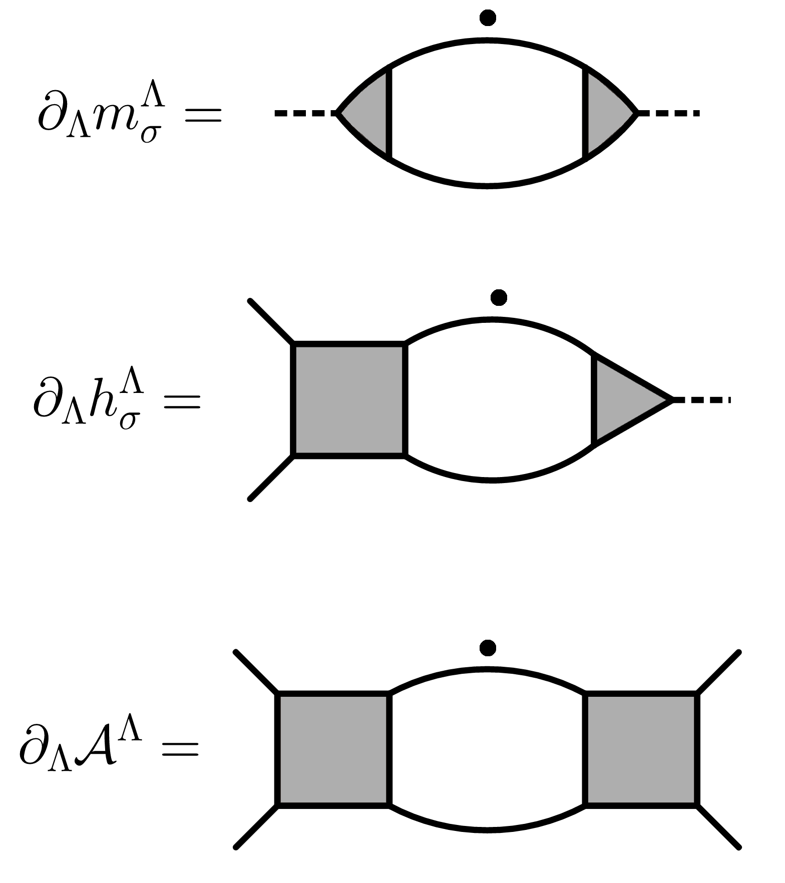
Figure 1: Schematic representation of flow equations for the mass and the couplings in the longitudinal channel. Full lines represent Nambu matrix propagators, triangles the Yukawa coupling $h_{\sigma}$ and squares the residual interaction $\mathcal{A}$. The black dots over fermionic legs represent full derivatives with respect to the scale $\Lambda$.

In the transverse channel, the equations have the same structure and can be integrated in the same way. Their solutions read

$$\Phi^{\Lambda}=\left[1-\widetilde{\mathcal{Q}}^{\Lambda_{s}}\Pi_{22}^{\Lambda}\right]^{-1}\widetilde{\mathcal{Q}}^{\Lambda_{s}},$$ (43)

$$h_{\pi}^{\Lambda}=\left[1-\widetilde{\mathcal{Q}}^{\Lambda_{s}}\Pi_{22}^{\Lambda}\right]^{-1}\widetilde{h}^{\Lambda_{s}},$$ (44)

$$m_{\pi}^{\Lambda}=\widetilde{m}^{\Lambda_{s}}-\left[\widetilde{h}^{\Lambda_{s}}\right]^{T}\Pi_{22}^{\Lambda}\,h_{\pi}^{\Lambda}.$$ (45)

Eq. (45) provides the mass of the transverse mode, which, according to the Goldstone theorem, must be zero. We will show later that this is indeed fulfilled.

It is worthwhile to point out that the combinations

$$\begin{split}&\frac{h_{\sigma}^{\Lambda}\left[h_{\sigma}^{\Lambda}\right]^{T}}{m_{\sigma}^{\Lambda}}+\mathcal{A}^{\Lambda}\\ &\frac{h_{\pi}^{\Lambda}\left[h_{\pi}^{\Lambda}\right]^{T}}{m_{\pi}^{\Lambda}}+\Phi^{\Lambda}\end{split}$$ (46)

obey the same flow equations, Eqs. (12) and (13), as the vertices in the fermionic formalism and share the same initial conditions. Therefore the solutions for these quantities coincide with expressions (15) and (22), respectively. Within this equivalence, it is interesting to express the irreducible vertex $\widetilde{V}^{\Lambda_{s}}$ of Eq. (18) in terms of the quantities, $\mathcal{Q}^{\Lambda_{s}}$, $h^{\Lambda_{s}}$ and $m^{\Lambda_{s}}$, introduced in the factorization in Eq. (26):

$$\widetilde{V}^{\Lambda_{s}}=\frac{\widetilde{h}^{\Lambda_{s}}\left[\widetilde{h}^{\Lambda_{s}}\right]^{T}}{\widetilde{m}^{\Lambda_{s}}}+\widetilde{\mathcal{Q}}^{\Lambda_{s}},$$ (47)

where $\widetilde{\mathcal{Q}}^{\Lambda_{s}}$, $\widetilde{h}^{\Lambda_{s}}$ and $\widetilde{m}^{\Lambda_{s}}$ were defined in Eqs. (38), (40) and (42). For a proof see Appendix B. Relation (47) is of particular interest because it states that when the full vertex is expressed as in Eq. (26), then the irreducible one will obey a similar decomposition, where the bosonic propagator, Yukawa coupling and residual two fermion interaction are replaced by their ”reduced” counterparts. This relation holds even for $q\neq 0$.

V.3 Ward identity for the gap and Goldstone theorem

We now focus on the flow of the fermionic gap and the bosonic expectation value and express a relation that connects them. Their flow equations are given by (see Appendix A)

$$\partial_{\Lambda}\alpha^{\Lambda}=\frac{1}{m_{\sigma}^{\Lambda}}\left[h_{\sigma}^{\Lambda}\right]^{T}\widetilde{\partial}_{\Lambda}F^{\Lambda},$$ (48)

and

$$\begin{split}\partial_{\Lambda}\Delta^{\Lambda}&=\partial_{\Lambda}\alpha^{\Lambda}\,h_{\sigma}^{\Lambda}+\mathcal{A}^{\Lambda}\widetilde{\partial}_{\Lambda}F^{\Lambda}\\ &=\left[\frac{h_{\sigma}^{\Lambda}\left[h_{\sigma}^{\Lambda}\right]^{T}}{m_{\sigma}^{\Lambda}}+\mathcal{A}^{\Lambda}\right]\widetilde{\partial}_{\Lambda}F^{\Lambda},\end{split}$$ (49)

with $F^{\Lambda}$ given by Eq. (20). In Fig. 2 we show a pictorial representation.

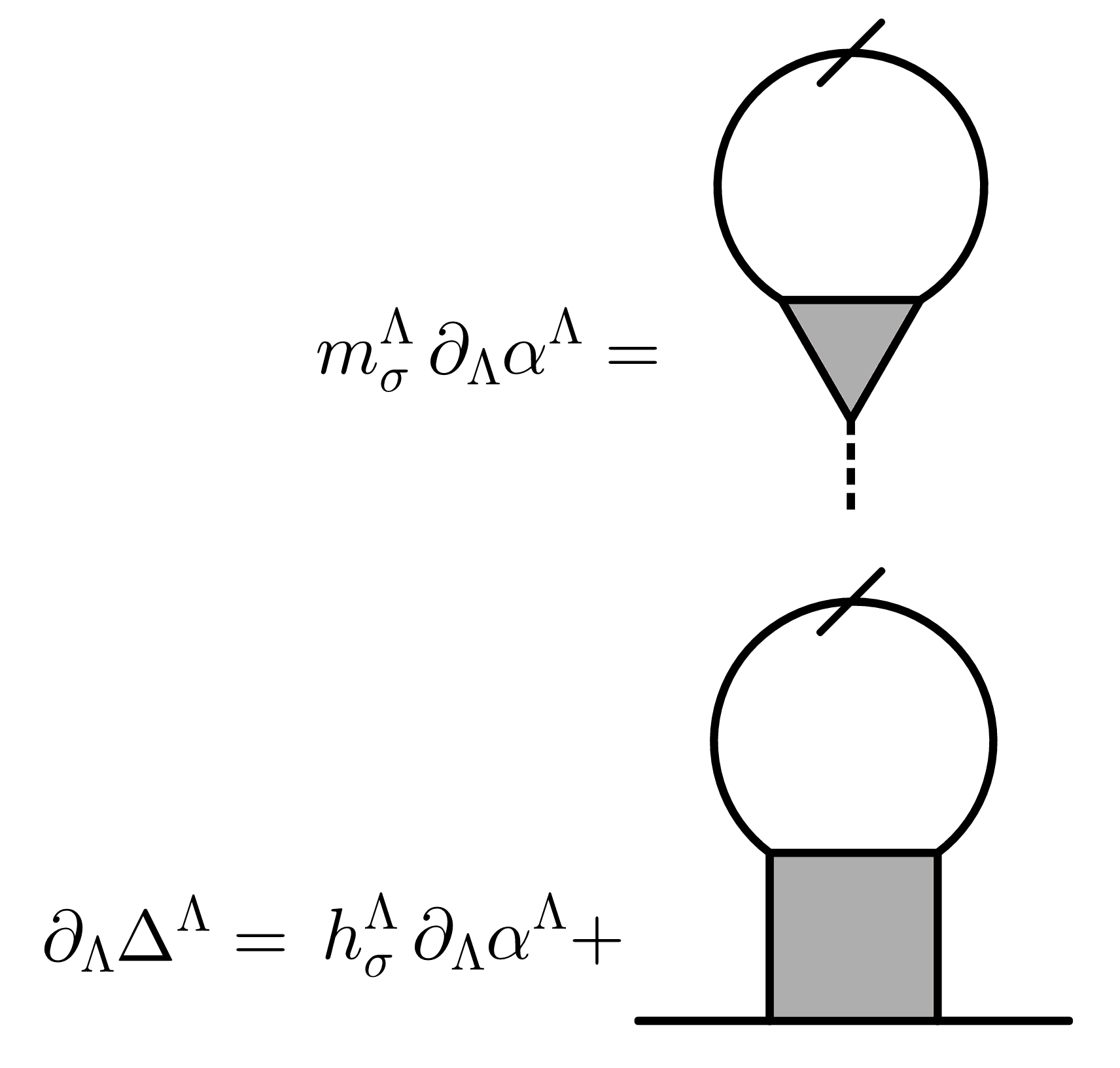
Figure 2: Schematic representation of flow equations for the bosonic expectation value $\alpha^{\Lambda}$ and fermionic gap $\Delta^{\Lambda}$. Besides the slashed lines, representing Nambu matrix propagators with a scale derivative acting only on the regulator, the conventions for the symbols are the same as in Fig. 1.

Eq. (48) can be integrated, with the help of the previously obtained results for $\mathcal{A}$, $h_{\sigma}$ and $m_{\sigma}$, yielding

$$\alpha^{\Lambda}=\frac{1}{\widetilde{m}^{\Lambda_{s}}}\left[\widetilde{h}^{\Lambda_{s}}\right]^{T}F^{\Lambda}.$$ (50)

In the last line of Eq. (49), as previously discussed, the object in angular brackets equals the full vertex $V_{\mathcal{A}}$ of the fermionic formalism. Thus, integration of the gap equation is possible and the result is simply Eq. (21) of the fermionic formalism. However, if we now insert the expression in Eq. (47) for the irreducible vertex within the ”fermionic” form (Eq. (21)) of the gap equation, and use relation (23), we get:

$$\Delta^{\Lambda}(k)=\alpha^{\Lambda}h_{\pi}^{\Lambda}(k).$$ (51)

This equation is the Ward identity for the mixed boson-fermion system related to the global U(1) symmetry [26]. In Appendix C we propose a self consistent loop for the calculation of $\alpha$, $h_{\pi}$, through Eqs. 50 and 44, and subsequently the superfluid gap $\Delta$. Let us now come back to the question of the Goldstone theorem. For the mass of the Goldstone boson to be zero, it is necessary for Eq. (45) to vanish. We show that this is indeed the case. With the help of Eq. (23), we can reformulate the equation for the transverse mass in the form

$$\begin{split}m^{\Lambda}_{\pi}&=\widetilde{m}^{\Lambda_{s}}-\int_{k}\widetilde{h}^{\Lambda_{s}}(k)F^{\Lambda}(k)\frac{h^{\Lambda}_{\pi}(k)}{\Delta^{\Lambda}(k)}\\ &=\widetilde{m}^{\Lambda_{s}}-\frac{1}{\alpha^{\Lambda}}\int_{k}\widetilde{h}^{\Lambda_{s}}(k)F^{\Lambda}(k),\end{split}$$ (52)

where the Ward Identity $\Delta=\alpha h_{\pi}$ was applied in the last line. We see that the expression for the Goldstone boson mass vanishes when $\alpha$ obeys its self consistent equation, Eq. (50). This proves that our truncation of flow equations fulfills the Goldstone theorem.
blackConstructing a truncation of the fRG flow equations which fulfills the Ward identities and the Goldstone theorem is, in general, a nontrivial task. In Ref. [25], in which the order parameter fluctuations have been included on top of the Hartree-Fock solution, no distinction has been made between the longitudinal and transverse Yukawa couplings and the Ward identity (51) as well as the Goldstone theorem have been enforced by construction, by calculating the gap and the bosonic expectation values from them rather than from their flow equations. Similarly, in Ref. [26], in order for the flow equations to fulfill the Goldstone theorem, it was necessary to impose $h_{\sigma}=h_{\pi}$ and use only the flow equation of $h_{\pi}$ for both Yukawa couplings. Within the present approach, due to the mean-field-like nature of the truncation, the Ward identity (51) and the Goldstone theorem are automatically fulfilled by the flow equations.

V.4 Equivalence of bosonic and fermionic formalisms

As we have proven in the previous sections, within the MF approximation the fully fermionic formalism of Sec. IV and the bosonized approach introduced in the present section provide the same results for the superfluid gap and for the effective two fermion interactions. Notwithstanding the formal equivalence, the bosonic formulation relies on a further requirement. In Eqs. (43) and (44) we assumed the matrix $\left[1-\widetilde{\mathcal{Q}}^{\Lambda_{s}}\Pi_{22}^{\Lambda}\right]$ to be invertible. This statement is exactly equivalent to assert that the two fermion residual interaction $\Phi$ remains finite. Otherwise the Goldstone mode would lie in this coupling and not (only) in the Hubbard-Stratonovich boson. This fact cannot occur if the flow is stopped at a scale $\Lambda_{s}$ coinciding with the critical scale $\Lambda_{c}$ at which the (normal) bosonic mass $m^{\Lambda}$ turns zero, but it could take place if one considers symmetry breaking in more than one channel. In particular, if one allows the system to develop two different orders and stops the flow when the mass of one of the two associated bosons becomes zero, it could happen that, within a MF approximation for both order types, the appearance of a finite gap in the first channel makes the two fermion transverse residual interaction in the other channel diverging. In that case one can apply the technique of the flowing bosonization [31, 32], by reassigning to the bosonic sector the (most singular part of the) two fermion interactions that are generated during the flow. It can be proven that also this approach gives the same results for the gap and the effective fermionic interactions in Eq. (46) as the fully fermionic formalism.

VI Vertex bosonization

In this section we present a systematic procedure to extract the quantities in Eq. (26) from a given vertex, within an approximate framework. The full vertex in the symmetric phase can be written as [70, 71]

$$\begin{split}V^{\Lambda}(k_{1},k_{2},k_{3})&=V^{\Lambda_{\text{ini}}}(k_{1},k_{2},k_{3})\\ &+\phi^{\Lambda}_{p}\left(k_{1},k_{3};k_{1}+k_{2}\right)\\ &-\phi^{\Lambda}_{m}\left(k_{1},k_{2};k_{2}-k_{3}\right)\\ &-\frac{1}{2}\phi^{\Lambda}_{m}\left(k_{1},k_{2};k_{3}-k_{1}\right)\\ &+\frac{1}{2}\phi^{\Lambda}_{c}\left(k_{1},k_{2};k_{3}-k_{1}\right),\end{split}$$ (53)

where $V^{\Lambda_{\text{ini}}}$ is the vertex at the initial scale, and we call $\phi_{p}$ pairing channel, $\phi_{m}$ magnetic channel and $\phi_{c}$ charge channel. Each of this functions depends on a bosonic and two fermionic variables. Within the so called 1-loop approximation, where one neglects the 3-fermion coupling in Eq. (5), in the Katanin scheme [68], or in more involved schemes, such as the 2-loop [14] or the multiloop [41, 42], one is able to assign one or more of the terms of the flow equation (5) for $V^{\Lambda}$ to each of the channels, in a way that their last bosonic argument enters only parametrically in the formulas. This is the reason why the decomposition in Eq. (53) is useful. The vertex at the initial scale can be set equal to the bare (sign-reversed) Hubbard interaction $-U$ in a weak-coupling approximation, or as in the recently introduced DMF²RG scheme, to the vertex computed via DMFT [45, 46].

In order to simplify the treatment of the dependence on fermionic spatial momenta of the various channels, one often introduces a complete basis of Brillouin zone form factors $\{f^{\ell}_{\mathbf{k}}\}$ and expands each channel in this basis [72]

$$\begin{split}\phi^{\Lambda}_{X}(k,k^{\prime};q)=\sum_{\ell\ell^{\prime}}\phi^{\Lambda}_{X,\ell\ell^{\prime}}(\nu,\nu^{\prime};q)f^{\ell}_{\mathbf{k}+(\text{sgn}X)\mathbf{q}/2}\,f^{\ell^{\prime}}_{\mathbf{k^{\prime}}-\mathbf{q}/2},\end{split}$$ (54)

with $X=p$, $m$ or $c$, and $\text{sgn}\,p=-1$, $\text{sgn}\,c=\text{sgn}\,m=+1$. For practical calculations the above sum is truncated to a finite number of form factors and often only diagonal terms, $\ell=\ell^{\prime}$, are considered. Within the form factor truncated expansion, one is left with the calculation of a finite number of channels that depend on a bosonic ”$d$+1 momentum” $q=(\mathbf{q},\Omega)$ and two fermionic Matsubara frequencies $\nu$ and $\nu^{\prime}$.

We will now show how to obtain the decomposition introduced in Eq. (26) within the form factor expansion. We focus on only one of the channels in Eq. (53), depending on the type of order we are interested in, and factorize its dependence on the two fermionic Matsubara frequencies. We introduce the so called channel asymptotics, that is the functions that describe the channels for large $\nu$, $\nu^{\prime}$. From now on we adopt the shorthand $\lim_{\nu\rightarrow\infty}g(\nu)=g(\infty)$ for whatever $g$, function of $\nu$. By considering only diagonal terms in the form factor expansion in Eq. (54), we can write the channels as [73]:

$$\begin{split}\phi_{X,\ell}^{\Lambda}(\nu,\nu^{\prime};q)&=\mathcal{K}_{X,\ell}^{(1)\Lambda}(q)+\mathcal{K}_{X,\ell}^{(2)\Lambda}(\nu;q)\\ &+\overline{\mathcal{K}}_{X,\ell}^{(2)\Lambda}(\nu^{\prime};q)+\delta\phi^{\Lambda}_{X,\ell}(\nu,\nu^{\prime};q),\end{split}$$ (55)

with

$$\begin{split}&\mathcal{K}_{X,\ell}^{(1)\Lambda}(q)=\phi_{X,\ell}^{\Lambda}(\infty,\infty;q)\\ &\mathcal{K}_{X,\ell}^{(2)\Lambda}(\nu;q)=\phi_{X,\ell}^{\Lambda}(\nu,\infty;q)-\mathcal{K}_{X,\ell}^{(1)\Lambda}(q)\\ &\overline{\mathcal{K}}_{X,\ell}^{(2)\Lambda}(\nu^{\prime};q)=\phi_{X,\ell}^{\Lambda}(\infty,\nu^{\prime};q)-\mathcal{K}_{X,\ell}^{(1)\Lambda}(q)\\ &\delta\phi^{\Lambda}_{X,\ell}(\nu,\infty;q)=\delta\phi^{\Lambda}_{X,\ell}(\infty,\nu^{\prime};q)=0.\end{split}$$ (56)

According to Ref. [73], these functions are related to physical quantities. $\mathcal{K}_{X,\ell}^{(1)}$ turns out to be proportional to the relative susceptibility and the combination $\mathcal{K}_{X,\ell}^{(1)}+\mathcal{K}_{X,\ell}^{(2)}$ (or $\mathcal{K}_{X,\ell}^{(1)}+\overline{\mathcal{K}}_{X,\ell}^{(2)}$) to the so called boson-fermion vertex, that describes both the response of the Green’s function to an external field [74] and the coupling between a fermion and an effective boson. In principle one should be able to calculate the above quantities diagrammatically (see Ref. [73] for the details) without performing any limit. However, it is well known how fRG truncations, in particular the 1-loop approximation, do not properly weight all the Feynman diagrams contributing to the vertex, so that the diagrammatic calculation and the high frequency limit give two different results. To keep the property in the last line of Eq. (56), we choose to perform the limits. We rewrite Eq. (55) in the following way:

$$\begin{split}&\phi_{X,\ell}^{\Lambda}(\nu,\nu^{\prime};q)=\\ &=\frac{\left[\mathcal{K}_{X,\ell}^{(1)\Lambda}+\mathcal{K}_{X,\ell}^{(2)\Lambda}\right]\left[\mathcal{K}_{X,\ell}^{(1)\Lambda}+\overline{\mathcal{K}}_{X,\ell}^{(2)\Lambda}\right]}{\mathcal{K}_{X,\ell}^{(1)\Lambda}}+\mathcal{R}_{X,\ell}^{\Lambda}\\ &=\frac{\phi_{X,\ell}^{\Lambda}(\nu,\infty;q)\phi_{X,\ell}^{\Lambda}(\infty,\nu^{\prime};q)}{\phi_{X,\ell}^{\Lambda}(\infty,\infty;q)}+\mathcal{R}_{X,\ell}^{\Lambda}(\nu,\nu^{\prime};q),\end{split}$$ (57)

where we have made the frequency and momentum dependencies explicit only in the second line and we have defined

$$\mathcal{R}_{X,\ell}^{\Lambda}(\nu,\nu^{\prime};q)=\delta\phi^{\Lambda}_{X,\ell}(\nu,\nu^{\prime};q)-\frac{\mathcal{K}_{X,\ell}^{(2)\Lambda}(\nu;q)\overline{\mathcal{K}}_{X,\ell}^{(2)\Lambda}(\nu^{\prime};q)}{\mathcal{K}_{X,\ell}^{(1)\Lambda}(q)}.$$ (58)

From the definitions given above, it is obvious that the rest function $\mathcal{R}_{X,\ell}$ decays to zero in all frequency directions.

Since the first term of Eq. (57) is separable by construction, we choose to identify this term with the first one of Eq. (26). Indeed, in many cases the vertex divergence is manifest already in the asymptotic $\mathcal{K}_{X,\ell}^{(1)\Lambda}$, that we recall to be proportional to the susceptibility of the channel. There are however situations in which the functions $\mathcal{K}^{(1)}$ and $\mathcal{K}^{(2)}$ are zero even close to an instability in the channel, an important example being the d-wave superconducting instability in the repulsive Hubbard model. In general, this occurs for those channels that, within a Feynman diagram expansion, cannot be constructed with a ladder resummation with the bare vertex. In the Hubbard model, due to the locality of the bare interaction, this happens for every $\ell\neq 0$, that is for every term in the form factor expansion different than the s-wave contribution. In this case one should adopt a different approach and, for example, replace the limits to infinity in Eq. (57) by some given values of the Matsubara frequencies, $\pm\pi T$ for example.

VII Results for the attractive Hubbard model at half-filling

In this section we report some exemplary results of the equations derived within the bosonic formalism, for the attractive two-dimensional Hubbard model. We focus on the half-filled case. For pure nearest neighbors hopping with amplitude $-t$, the band dispersion $\xi_{\mathbf{k}}$ is given by

$$\xi_{\mathbf{k}}=-2t\left(\cos k_{x}+\cos k_{y}\right)-\mu,$$ (59)

with $\mu=0$ at half-filling. We choose the onsite attraction and the temperature to be $U=-4t$ and $T=0.1t$. All results are presented in units of the hopping parameter $t$.

VII.1 Symmetric phase

In the symmetric phase, in order to run a fRG flow, we introduce the $\Omega$-regulator [70]

$$R^{\Lambda}(k)=\left(i\nu-\xi_{\mathbf{k}}\right)\frac{\Lambda^{2}}{\nu^{2}},$$ (60)

so that the initial scale is $\Lambda_{\text{init}}=+\infty$ (fixed to a large number in the numerical calculation) and the final one $\Lambda_{\text{fin}}=0$. We choose a 1-loop truncation, that is we neglect the last term of Eq. (5), and use the decomposition in Eq. (53) with a form factor expansion. We truncate Eq. (54) only to the first term, that is we use only s-wave, $f^{(0)}_{\mathbf{k}}\equiv 1$, form factors. Within these approximations, the vertex reads

$$\begin{split}V^{\Lambda}(&k_{1},k_{2},k_{3})=-U+\mathcal{P}^{\Lambda}_{\nu_{1}\nu_{3}}(k_{1}+k_{2})\\ -&\mathcal{M}^{\Lambda}_{\nu_{1}\nu_{2}}(k_{2}-k_{3})\\ -&\frac{1}{2}\mathcal{M}^{\Lambda}_{\nu_{1}\nu_{2}}(k_{3}-k_{1})+\frac{1}{2}\mathcal{C}^{\Lambda}_{\nu_{1}\nu_{2}}(k_{3}-k_{1}),\end{split}$$ (61)

where $\mathcal{P}$, $\mathcal{M}$, $\mathcal{C}$, are referred as pairing, magnetic and charge channel, respectively. Furthermore, we focus only on the spin-singlet component of the pairing (the triplet one is very small in the present parameter region), so that we require the pairing channel to obey [75]

$$\mathcal{P}^{\Lambda}_{\nu\nu^{\prime}}(q)=\mathcal{P}^{\Lambda}_{\Omega-\nu,\nu^{\prime}}(q)=\mathcal{P}^{\Lambda}_{\nu,\Omega-\nu^{\prime}}(q),$$ (62)

with $q=(\mathbf{q},\Omega)$. The initial condition for the vertex reads

$$V^{\Lambda_{\text{init}}}(k_{1},k_{2},k_{3})=-U,$$ (63)

so that $\mathcal{P}^{\Lambda_{\text{init}}}=\mathcal{M}^{\Lambda_{\text{init}}}=\mathcal{C}^{\Lambda_{\text{init}}}=0$. Neglecting the fermionic self-energy, $\Sigma^{\Lambda}(k)\equiv 0$, we run a flow for these three quantities until one (ore more) of them diverges. Under a technical point of view, each channel is computed by keeping 50 positive and 50 negative values for each of the three Matsubara frequencies (two fermionic, one bosonic) on which it depends. Frequency asymptotics are also taken into account, by following Ref. [73]. The momentum dependence of the channel is treated by discretizing with 38 patches the region $\mathcal{B}=\{(k_{x},k_{y}):0\leq k_{y}\leq k_{x}\leq\pi\}$ in the Brillouin zone and extending to the other regions by using lattice symmetries. The expressions of the flow equations are reported in Appendix D.

Due to particle-hole symmetry occurring at half-filling, pairing fluctuations at $\mathbf{q}=0$ combine with charge fluctuations at $\mathbf{q}=(\pi,\pi)$ to form an order parameter with SO(3) symmetry [76]. Indeed, with the help of a canonical particle-hole transformation, one can map the attractive half-filled Hubbard model onto the repulsive one. Within this duality, the SO(3)-symmetric magnetic order parameter is mapped onto the above mentioned combined charge-pairing order parameter and vice versa. This is the reason why we find a critical scale, $\Lambda_{c}$, at which both $\mathcal{C}((\pi,\pi),0)$ and $\mathcal{P}(\mathbf{0},0)$ diverge, as shown in Fig. 3. On a practical level, we define the stopping scale $\Lambda_{s}$ as the scale at which one (or more, in this case) channel exceeds $10^{3}t$. With our choice of parameters, we find that at $\Lambda_{s}\simeq 0.378t$ both $\mathcal{C}$ and $\mathcal{P}$ cross our threshold.

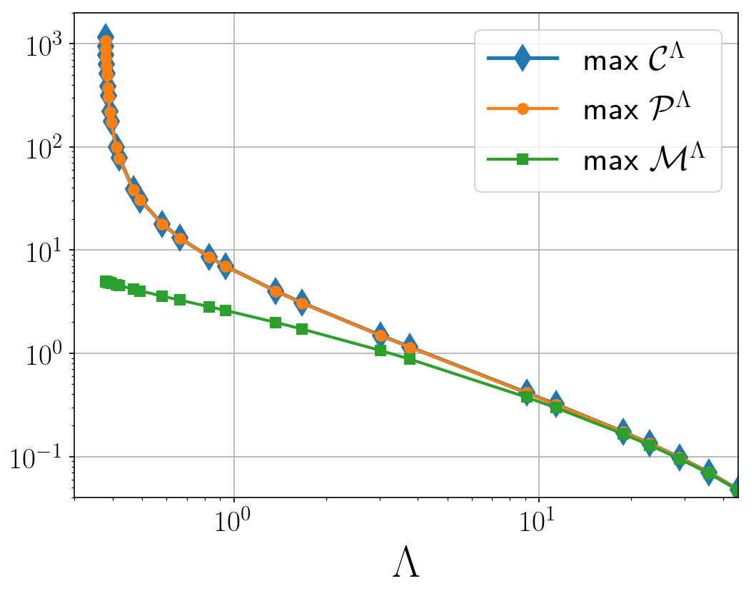
Figure 3: Flow of the maximum values of the pairing, magnetic and charge channel. The maximum value of the charge channel at zero frequency and momentum $(\pi,\pi)$ and the one for the pairing channel at $q=0$ coincide, within the numerical accuracy, and both exceed the threshold $10^{3}t$ at the stopping scale, signaling an instability to the formation of an order parameter given by any linear combination of the superfluid and the charge density wave ones.

In the SSB phase, we choose to restrict the ordering to the pairing channel, thus excluding the formation of charge density waves. This choice is always possible because we have the freedom to choose the ”direction” in which our order parameter points. Indeed, in the particle-hole dual repulsive model, our choice would be equivalent to choose the (antiferro-) magnetic order parameter to lie in the $xy$ plane. This choice is implemented by selecting the particle-particle channel as the only one contributing to the flow in the SSB phase, as exposed in Secs. IV and V.

In order to access the SSB phase with our bosonic formalism, we need to perform the decomposition in Eq. (26) for our vertex at $\Lambda_{s}$. Before proceeding, in order to be consistent with our form factor expansion in the SSB phase, we need to project $V$ in Eq. (61) onto the s-wave form factors, because we want the quantities in the ordered phase to be functions of Matsubara frequencies only. Therefore we define the total vertex projected onto s-wave form factors

$$\overline{V}^{\Lambda_{s}}_{\nu\nu^{\prime}}(q)=\int_{\mathbf{k},\mathbf{k}^{\prime}}V^{\Lambda_{s}}\hskip-2.84526pt\left(k,q-k,k^{\prime}\right).$$ (64)

Furthermore, since we are interested only in spin singlet pairing, we symmetrize it with respect to one of the two fermionic frequencies, so that in the end we are dealing with

$$V^{\Lambda_{s}}_{\nu\nu^{\prime}}(q)=\frac{\overline{V}^{\Lambda_{s}}_{\nu\nu^{\prime}}(q)+\overline{V}^{\Lambda_{s}}_{\nu,\Omega-\nu^{\prime}}(q)}{2}.$$ (65)

In order to extract the Yukawa coupling $h^{\Lambda_{s}}$ and bosonic propagator $m^{\Lambda_{s}}$, we employ the strategy described in Sec. VI. Here, however, instead of factorizing the pairing channel $\mathcal{P}^{\Lambda_{s}}$ alone, we subtract from it the bare interaction $U$. In principle, $U$ can be assigned both to the pairing channel, to be factorized, or to the residual two fermion interaction, giving rise to the same results in the SSB phase. However, when in a real calculation the vertices are calculated on a finite frequency box, it is more convenient to have the residual two fermion interaction $\mathcal{Q}^{\Lambda_{s}}$ as small as possible, in order to reduce finite size effects in the matrix inversions needed to extract the reduced couplings in Eqs. (38), (40) and (42), and in the calculation of $h_{\pi}$, in Eq. (44). Furthermore, since it is always possible to rescale the bosonic propagators and Yukawa couplings by a constant such that the vertex constructed with them (Eq. (57)) is invariant, we impose the normalization condition $h^{\Lambda_{s}}(\nu\rightarrow\infty;q)=1$. In formulas, we have

$$m^{\Lambda_{s}}(q)=\frac{1}{\mathcal{K}_{p,\ell=0}^{(1)\Lambda_{s}}(q)-U}=\frac{1}{\mathcal{P}^{\Lambda_{s}}_{\infty,\infty}(q)-U},$$ (66)

and

$$\begin{split}h^{\Lambda_{s}}(\nu;q)&=\frac{\mathcal{K}_{p,\ell=0}^{(2)\Lambda_{s}}(\nu;q)+\mathcal{K}_{p,\ell=0}^{(1)\Lambda_{s}}(q)-U}{\mathcal{K}_{p,\ell=0}^{(1)\Lambda_{s}}(q)-U}\\ &=\frac{\mathcal{P}^{\Lambda_{s}}_{\nu,\infty}(q)-U}{\mathcal{P}^{\Lambda_{s}}_{\infty,\infty}(q)-U}.\end{split}$$ (67)

The limits are numerically performed by evaluating the pairing channel at large values of the fermionic frequencies. The extraction of the factorizable part from the pairing channel minus the bare interaction defines the rest function

$$\mathcal{R}^{\Lambda_{s}}_{\nu\nu^{\prime}}(q)=\mathcal{P}^{\Lambda_{s}}_{\nu\nu^{\prime}}(q)-U-\frac{h^{\Lambda_{s}}(\nu;q)h^{\Lambda_{s}}(\nu^{\prime};q)}{m^{\Lambda_{s}}(q)},$$ (68)

and the residual two fermion interaction $\mathcal{Q}$

$$\begin{split}\mathcal{Q}^{\Lambda_{s}}_{\nu\nu^{\prime}}(q)=&\left[V^{\Lambda_{s}}_{\nu\nu^{\prime}}(q)-\mathcal{P}^{\Lambda_{s}}_{\nu\nu^{\prime}}(q)+U\right]+\mathcal{R}^{\Lambda_{s}}_{\nu\nu^{\prime}}(q)\\ =&V^{\Lambda_{s}}_{\nu\nu^{\prime}}(q)-\frac{h^{\Lambda_{s}}(\nu;q)h^{\Lambda_{s}}(\nu^{\prime};q)}{m^{\Lambda_{s}}(q)}.\end{split}$$ (69)

We are now in the position to extract the reduced couplings, $\widetilde{\mathcal{Q}}^{\Lambda_{s}}$, $\widetilde{h}^{\Lambda_{s}}$ and $\widetilde{m}^{\Lambda_{s}}$, defined in Eqs. (38), (40), (42). This is achieved by numerically inverting the matrix (we drop the $q$-dependence from now on, assuming always $q=0$)

$$\delta_{\nu\nu^{\prime}}+\mathcal{Q}^{\Lambda_{s}}_{\nu\nu^{\prime}}\,\chi^{\Lambda_{s}}_{\nu^{\prime}},$$ (70)

with

$$\chi^{\Lambda_{s}}_{\nu}=T\int_{\mathbf{k}}G_{0}^{\Lambda_{s}}(k)G_{0}^{\Lambda_{s}}(-k),$$ (71)

and

$$G_{0}^{\Lambda_{s}}(k)=\frac{1}{i\nu-\xi_{\mathbf{k}}+R^{\Lambda_{s}}(k)}=\frac{\nu^{2}}{\nu^{2}+\Lambda_{s}^{2}}\frac{1}{i\nu-\xi_{\mathbf{k}}}.$$ (72)

In Fig. 4 we show the results for the pairing channel minus the bare interaction, the rest function, the residual two fermion interaction $\mathcal{Q}$ and the reduced one $\widetilde{\mathcal{Q}}$ at the stopping scale. One can see that in the present parameter region the pairing channel (minus $U$) is highly factorizable. Indeed, despite the latter being very large because of the vicinity to the instability, the rest function $\mathcal{R}$ remains very small, a sign that the pairing channel is well described by the exchange of a single boson. Furthermore, thanks to our choice of assigning the bare interaction to the factorized part, as we see in Fig. 4, both $\mathcal{Q}$ and $\widetilde{\mathcal{Q}}$ possess frequency structures that arise from a background that is zero.

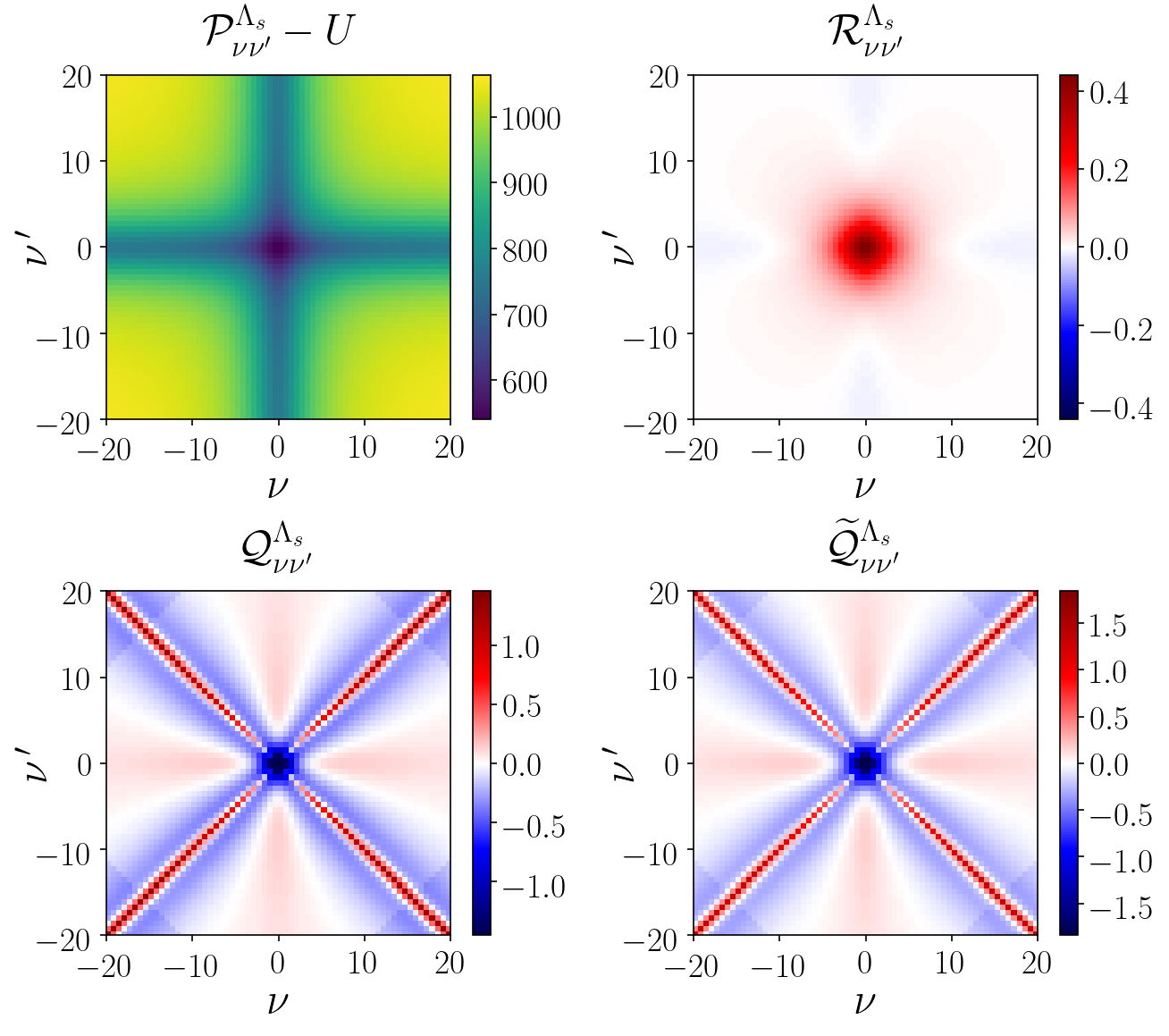
Figure 4: Couplings contributing to the total vertex at the stopping scale.
Upper left: pairing channel minus the bare interaction. At the stopping scale this quantity acquires very large values due to the vicinity to the pairing instability.
Upper right: rest function of the pairing channel minus the bare interaction. In the present regime the pairing channel is very well factorizable, giving rise to a small rest function.
Lower left: residual two fermion interaction. The choice of factorizing $\mathcal{P}^{\Lambda_{s}}-U$ instead of $\mathcal{P}^{\Lambda_{s}}$ alone makes the background of this quantity zero.
Lower right: reduced residual two fermion interaction. As well as the full one, this coupling has a zero background value, making calculations of couplings in the SSB phase more precise by reducing finite size effects in the matrix inversions.

Finally, the full bosonic mass at the stopping scale is close to zero, $m^{\Lambda_{s}}\simeq 10^{-3}$, due to the vicinity to the instability, while the reduced one is finite, $\widetilde{m}^{\Lambda_{s}}\simeq 0.237$.

VII.2 SSB Phase

In the SSB phase, instead of running the fRG flow, we employ the analytical integration of the flow equations described in Sec. V. On a practical level, we implement a solution of the loop described in Appendix C, that allows for the calculation of the bosonic expectation value $\alpha$, the transverse Yukawa coupling $h_{\pi}$ and subsequently the fermionic gap $\Delta$ through the Ward identity $\Delta=\alpha h_{\pi}$. In this section we drop the dependence on the scale, since we have reached the final scale $\Lambda_{\text{fin}}=0$. Note that, as exposed previously, in the half-filled attractive Hubbard model the superfluid phase sets in by breaking a SO(3) rather than a U(1) symmetry. This means that one should expect the appearance of two massless Goldstone modes. Indeed, besides the Goldstone boson present in the (transverse) particle-particle channel, another one appears in the particle-hole channel and it is related to the divergence of the charge channel at momentum $(\pi,\pi)$. However, within our choice of considering only superfluid order and within the MF approximation, this mode is decoupled from our equations.

Within our previously discussed choice of bosonizing $\mathcal{P}^{\Lambda_{s}}-U$ instead of $\mathcal{P}^{\Lambda_{s}}$ alone, the self consistent loop introduced in Appendix C converges extremely fast, 15 iterations for example are sufficient to reach a precision of $10^{-7}$ in $\alpha$. Once convergence is reached and the gap $\Delta(\nu)$ obtained, we are in the position to evaluate the remaining couplings introduced in Sec. V through their integrated flow equations. In Fig. 5 we show the computed frequency dependence of the gap. It interpolates between $\Delta_{0}=\Delta(\nu\rightarrow 0)$, its value at the Fermi level, and its asymptotic value, that equals the (signed reversed) bare interaction times the blackcondensate fraction $\langle\psi_{\downarrow}\psi_{\uparrow}\rangle=$$\int_{\mathbf{k}}\langle\psi_{-\mathbf{k},\downarrow}\psi_{\mathbf{k},\uparrow}\rangle$. $\Delta_{0}$ also represents the gap between the upper and lower Bogoliubov bands. Magnetic and charge fluctuations above the critical scale significantly renormalize the gap with respect to the Hartree-Fock calculation ($\widetilde{V}=-U$ in Eq. (21)), that in the present case coincides with Bardeen-Cooper-Schrieffer (BCS) theory. blackThis effect is reminiscent of the Gor’kov-Melik-Barkhudarov correction in weakly coupled superconductors [77]. The computed frequency dependence of the gap compares qualitatively well with Ref. [35], where a more sophisticated truncation of the flow equations has been carried out.
Since $\Delta$ is a spin singlet superfluid gap, and we have chosen $\alpha$ to be real, it obeys

$$\Delta(\nu)=\Delta(-\nu)=\Delta^{*}(-\nu),$$ (73)

where the first equality comes from the spin singlet nature and the second one from the time reversal symmetry of the effective action. Therefore, the imaginary part of the gap is always zero. By contrast, a magnetic gap would gain, in general, a finite (and antisymmetric in frequency) imaginary part.

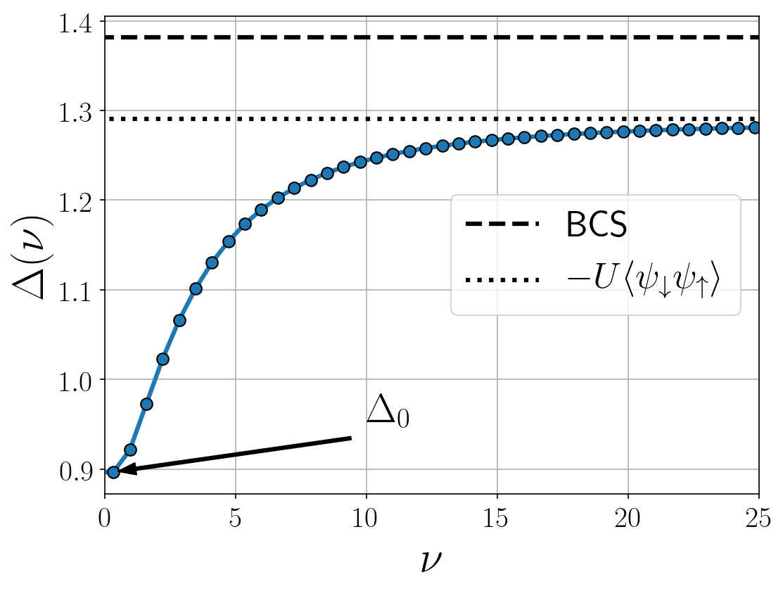
Figure 5: Frequency dependence of the superfluid gap. It interpolates between its value at the Fermi level, $\Delta_{0}$, and its asymptotic one. The dashed line marks the BCS value, while the dotted one $-U$ times the Cooper pair expectation value.

In Fig. 6 we show the results for the residual two fermion interactions in the longitudinal and transverse channels, together with the total effective interaction in the longitudinal channel, defined as

$$V_{\mathcal{A},\nu\nu^{\prime}}=\frac{h_{\sigma}(\nu)h_{\sigma}(\nu^{\prime})}{m_{\sigma}}+\mathcal{A}_{\nu\nu^{\prime}}.$$ (74)

The analogue of Eq. (74) for the transverse channel cannot be computed, because the transverse mass $m_{\pi}$ is zero, in agreement with the Goldstone theorem. The key result is that the residual interactions $\mathcal{A}_{\nu\nu^{\prime}}$ and $\Phi_{\nu\nu^{\prime}}$ inherit the frequency structures of $\widetilde{\mathcal{Q}}^{\Lambda_{s}}_{\nu\nu^{\prime}}$ and $\mathcal{Q}^{\Lambda_{s}}_{\nu\nu^{\prime}}$, respectively, and they are also close to them in values (compare with Fig. 4).

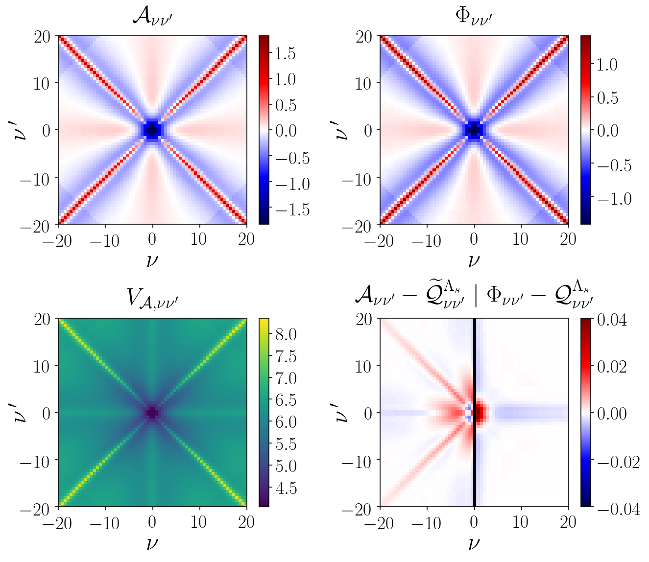
Figure 6: Effective interactions calculated in the SSB phase as functions of Matsubara frequencies.
Upper left: longitudinal residual two fermion interaction $\mathcal{A}$.
Upper right: transverse residual two fermion interaction $\Phi$.
Lower left: longitudinal effective two fermion interaction $V_{\mathcal{A}}$.
Lower right: longitudinal residual two fermion interaction $\mathcal{A}$ with its reduced counterpart $\widetilde{\mathcal{Q}}$ at the stopping scale subtracted (left), and transverse longitudinal residual two fermion interaction $\Phi$ minus its equivalent, $\mathcal{Q}$, at $\Lambda_{s}$ (right). Both quantities exhibit very small values, showing that $\mathcal{A}$ and $\Phi$ do not deviate significantly from $\widetilde{\mathcal{Q}}$ and $\mathcal{Q}$, respectively.

The same occurs for the Yukawa couplings, as shown in Fig. 7. Indeed, the calculated transverse coupling $h_{\pi}$ does not differ at all from the Yukawa coupling at the stopping scale $h^{\Lambda_{s}}$. In other words, if instead of solving the self consistent equations, one runs a flow in the SSB phase, the transverse Yukawa coupling will stay the same from $\Lambda_{s}$ to $\Lambda_{\text{fin}}$. Furthermore, the longitudinal coupling $h_{\sigma}$ develops a dependence on the frequency which does not differ significantly from the one of $\widetilde{h}^{\Lambda_{s}}$.

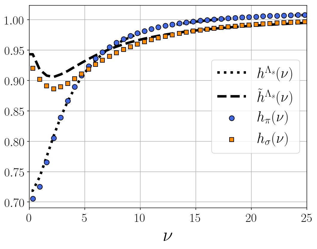
Figure 7: Frequency dependence of Yukawa couplings both at the stopping scale $\Lambda_{s}$ and in the SSB phase. While $h_{\pi}$ coincides with $h^{\Lambda_{s}}$, the longitudinal coupling $h_{\sigma}$ does not differ significantly from the reduced one at the stopping scale, $\widetilde{h}^{\Lambda_{s}}$. The continuous lines for $h^{\Lambda_{s}}$ and $\widetilde{h}^{\Lambda_{s}}$ are an interpolation through the data calculated on the Matsubara frequencies.

This feature, at least for our choice of parameters, can lead to some simplifications in the flow equations of Sec. V. Indeed, when running a fRG flow in the SSB phase, one might let flow only the bosonic inverse propagators by keeping the Yukawa couplings and residual interactions fixed at their values, reduced or not, depending on the channel, at the stopping scale. This fact can be crucial to make computational costs lighter when including bosonic fluctuations of the order parameter, which, similarly, do not significantly renormalize Yukawa couplings in the SSB phase [26, 25]. black

VII.3 Gap and condensate fraction dependence on the coupling

In this section, we carry out an analysis of the dependence of the zero-frequency gap $\Delta_{0}$ on the coupling $U$. In order to obtain a zero temperature estimate, we perform a finite temperature calculation and check that the condition $\Delta_{0}>T$ is fulfilled. In fact, when this is the case, the superfluid gap is not expected to change significantly by further lowering the temperature, at least within a MF-like calculation.

In Fig. 8, we show the zero-frequency extrapolation of the superfluid gap and the bosonic expectation value $\alpha$ to be compared with the BCS (mean-field) result. The inclusion of magnetic and charge correlations above the stopping scale $\Lambda_{s}$ renormalizes $\Delta_{0}$ compared to the BCS result. In particular, as proven by second order perturbation theory in Ref. [77], even in the $U\rightarrow 0$ limit the ratio between the ground state gap and its BCS result is expected to be smaller than 1 due to particle-hole fluctuations. Differently, $\alpha$ does not deviate significantly from the mean-field result, as this quantity is not particularly influenced by magnetic and charge fluctuations, but rather by fluctuations of the order parameter, which, in particular at strong coupling, can significantly reduce it [25]. In the present approach, we include the effect of particle-hole fluctuations and we tackle the frequency dependence of the gap, which are not treated in Refs. [25, 22] (which focus on the BEC-BCS crossover in the continuum in 3 dimensions), and [26] (2-dimensional lattice model). In these works, however, fluctuations of the order parameter, which are not included in our method, are taken into account. In Ref. [35], both particle-hole and order parameter fluctuations, together with the gap frequency dependence, are treated in a rather complicated fRG approach to the 2D attractive Hubbard model, where, however, the Goldstone theorem and the Ward identity turn out to be violated to some extent. We believe our approach to represent a convenient starting point on top of which one can include fluctuations in a systematic manner in order to fulfill the above mentioned fundamental constraints.

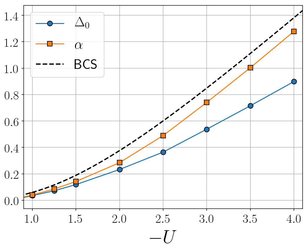
Figure 8: blackLow temperature estimate of the ground state superfluid gap $\Delta_{0}$ and bosonic expectation value $\alpha$ as a function of the coupling $U$. For $|U|>2t$, the calculations have been performed at $T=0.1t$, while for $t\leq|U|\leq 2t$ we have chosen $T=0.01t$. Results for $|U|<t$ are not shown because the temperature at which $\Delta_{0}>T$ is fulfilled is hardly reachable by our numerics. The dashed line shows the BCS (for which $\Delta_{0}=\alpha$) zero temperature result.

Furthermore, it is interesting to consider the coupling dependence of the condensate fraction $\langle\psi_{\downarrow}\psi_{\uparrow}\rangle$. Within mean-field theory, it evolves from an exponentially small value at weak coupling to $\frac{1}{2}$ at strong coupling, indicating that all the fermions are bound in bosonic pairs which condense. This is an aspect of the well-known paradigm of the BEC-BCS crossover [1, 2, 3]. At half filling, by including quantum fluctuations in the strong coupling regime, it is known that the condensate fraction will be reduced to a value of 0.3, as it has been obtained from the spin wave theory for the Heisenberg model [78], on which the particle-hole symmetric attractive Hubbard model can be mapped at large $U$. Within our approach, the condensate fraction is given by

$$\langle\psi_{\downarrow}\psi_{\uparrow}\rangle=-\lim_{\nu\rightarrow\infty}\frac{\Delta(\nu)}{U}=-\frac{\alpha}{U},$$ (75)

where in the last line we have used the Ward identity (51) and the fact that $h_{\pi}\rightarrow 1$ for $\nu\rightarrow\infty$. In Fig. 9 we show the computed condensate fraction and we compare it with the BCS result and with auxiliary field quantum Monte Carlo (AFQMC) data, taken from Ref. [62]. At weak coupling ($U=-2t$) we find a good agreement with AFQMC. This is due to the facts that in this regime the order parameter fluctuations, which we do no treat, are weaker, and that the stopping scale $\Lambda_{s}$ is small and therefore particle-hole fluctuations are better included. At moderate couplings ($U=-3t$, $-4t$) the distance from Monte Carlo data increases due to the increasing strength of fluctuations, the larger stopping scales and the reduction of accuracy of the 1-loop truncation performed in the symmetric phase.

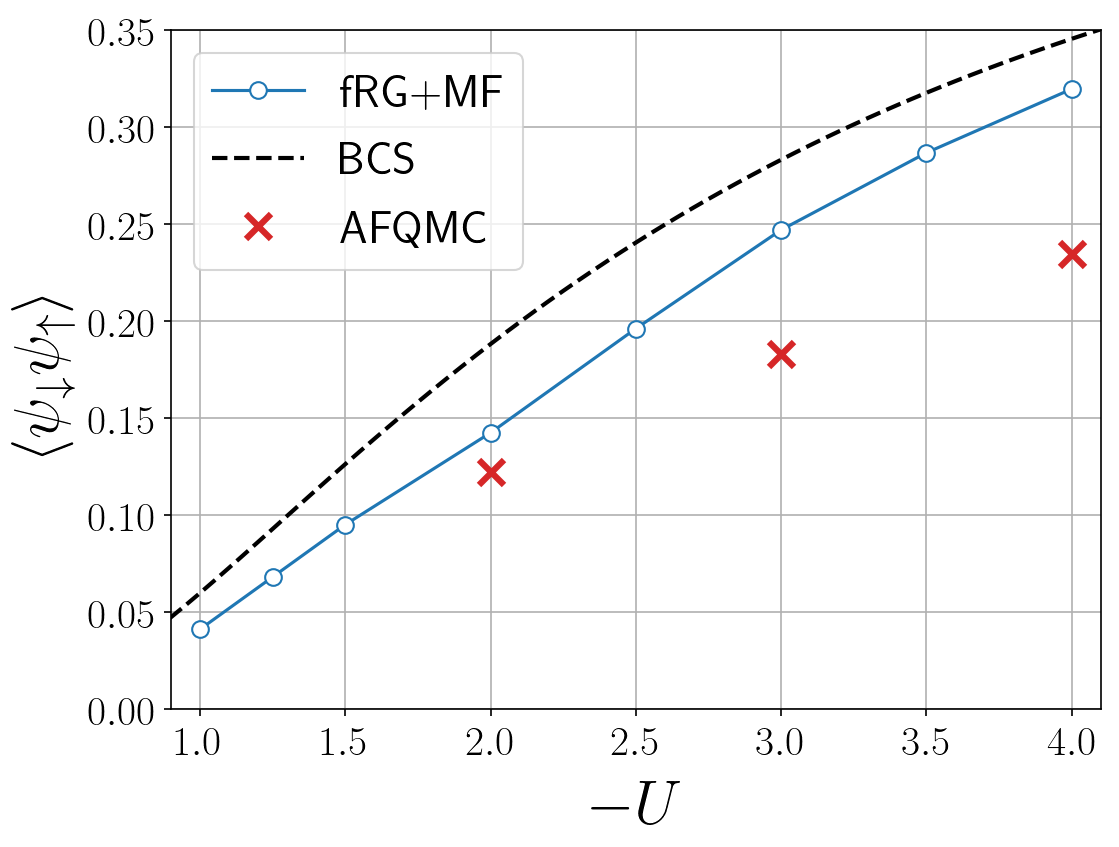
Figure 9: blackCondensate fraction $\langle\psi_{\downarrow}\psi_{\uparrow}\rangle$ vs coupling $U$. We indicate the present approach as fRG+MF, and we compare it with BCS theory and AFQMC data, taken from Ref. [62].

VIII Conclusion

We have introduced a truncation of fRG flow equations which, with the introduction of a Hubbard-Stratonovich boson, has been proven to be equivalent to the MF equations obtained in Refs. [39, 40]. These flow equations satisfy fundamental requirements such as the Goldstone theorem and the Ward identities associated with global symmetries, and can be integrated analytically, reducing the calculation of correlation functions in the SSB phase to a couple of self consistent equations for the bosonic expectation value $\alpha$ and the transverse Yukawa coupling $h_{\pi}$. A necessary step to perform the Hubbard-Stratonovich transformation, on which our method relies, is to extract a factorizable dependence on fermionic variables $k$ and $k^{\prime}$ from the vertex at the critical scale. A strategy to accomplish this goal has been suggested for a vertex whose dependence on spatial momenta $\mathbf{k}$ and $\mathbf{k}^{\prime}$ is treated by a form factor expansion, making use of the vertex asymptotics introduced in Ref. [73]. Furthermore, we have tested the feasibility and efficiency of our method on a prototypical model, namely the half-filled attractive Hubbard model in two dimensions, focusing on frequency dependencies of the two fermion interactions, Yukawa couplings and fermionic gap. We have found a good convergence of the iterative scheme proposed. The remaining couplings introduced in our method have been computed after the loop convergence from their integrated flow equations. blackMoreover, we have analyzed the dependence of the gap and of the condensate fraction on the coupling $U$, by comparing our method with previous fRG works and with quantum Monte Carlo data.

Our method leaves room for applications and extensions. First, one can directly apply the MF method, as formulated in this paper, to access the SSB phase in those calculations for which the dependencies on fermionic momenta and/or frequencies cannot be neglected. Some examples are the fRG calculations with a full treatment of fermionic frequencies, within a 1-loop truncation [55], in the recent implementations of multiloop fRG [43, 15] or in the DMF²RG scheme [46]. These combinations can be applied to two- or three-dimensional systems. In the former case, even though in 2D order parameter fluctuations are expected to play a decisive role, our method can be useful to get a first, though approximate, picture of the phase diagram. Of particular relevance is the 2D repulsive Hubbard model, used in the context of high-Tc superconductors. An interesting system for the latter case, where bosonic fluctuations are expected to be less relevant, is the 3D attractive Hubbard model, which, thanks to modern techniques, can be experimentally realized in cold atoms setups.

Secondly, our method constitutes a convenient starting point for the inclusion of bosonic fluctuations of the order parameter, as done for example in Refs. [32, 26], with the full dependence of the gap, Yukawa couplings and vertices on the fermionic momenta and/or frequencies being kept. In particular, by providing the Hubbard-Stratonovich boson with its own regulator, our MF-truncation of flow equations can be extended to include order parameter fluctuations, which in two spatial dimensions and at finite temperature restore the symmetric phase, in agreement with the Mermin-Wagner theorem. One may also adapt the bosonic field at every fRG step through the flowing bosonization [31, 32]. This can be done by keeping the full frequency dependence of the vertex and Yukawa coupling, by applying the strategy discussed in Sec. VI to the flow equation for the vertex.

Finally, our MF method does not necessarily require a vertex coming from a fRG flow. In particular, one can employ the DMFT vertex, extract the pairing channel [75] (or any other channel in which symmetry breaking occurs) from it, and apply the same strategy as described in this paper to extract Yukawa and other couplings. This application can be useful to compute those transport quantities [79] and response functions in the SSB phase which, within the DMFT, require a calculation of vertex corrections [44]. The anomalous vertices can be computed also at finite $q$ with a simple generalization of our formulas.

Appendix A Derivation of flow equations in the bosonic formalism

In this section we will derive the flow equations used in Sec. V.

We consider only those terms in which the dependence on the center of mass momentum $q$ is fixed to zero by the topology of the relative diagram or that depend only parametrically on it. These diagrams are the only ones necessary to reproduce the MF approximation.

The flow equations will be derived directly from the Wetterich equation (2), with a slight modification, since we have to keep in mind that the bosonic field $\phi$ acquires a scale dependence due to the scale dependence of its expectation value. The flow equation reads (for real $\alpha^{\Lambda}$):

$$\partial_{\Lambda}\Gamma^{\Lambda}=\frac{1}{2}\widetilde{\partial}_{\Lambda}\text{Str}\ln\left[\mathbf{\Gamma}^{(2)\Lambda}+R^{\Lambda}\right]+\frac{\delta\Gamma^{\Lambda}}{\delta\sigma_{q=0}}\,\partial_{\Lambda}\alpha^{\Lambda},$$ (76)

where $\mathbf{\Gamma}^{(2)\Lambda}$ is the matrix of the second derivatives of the action with respect to the fields, the supertrace Str includes a minus sign when tracing over fermionic variables. The first equation we derive is the one for the flowing expectation value $\alpha^{\Lambda}$. This is obtained by requiring that the one-point function for $\sigma_{q}$ vanishes. Taking the $\sigma_{q}$ derivative in Eq. (76) and setting the fields to zero, we have

$$\begin{split}&\partial_{\Lambda}\Gamma^{(0,1,0)\Lambda}(q=0)\equiv\partial_{\Lambda}\frac{\delta\Gamma^{\Lambda}}{\delta\sigma_{q=0}}\bigg{\lvert}_{\Psi,\overline{\Psi},\sigma,\pi=0}\\ &=-\int_{k}h^{\Lambda}_{\sigma}(k;0)\,\widetilde{\partial}_{\Lambda}F^{\Lambda}(k)+m^{\Lambda}_{\sigma}(0)\,\partial_{\Lambda}\alpha^{\Lambda}=0,\end{split}$$ (77)

where we have defined

$$\Gamma^{(2n_{1},n_{2},n_{3})\Lambda}=\frac{\delta^{(2n_{1}+n_{2}+n_{3})}\Gamma^{\Lambda}}{\left(\delta\overline{\Psi}\right)^{n_{1}}\left(\delta\Psi\right)^{n_{1}}\left(\delta\sigma\right)^{n_{2}}\left(\delta\pi\right)^{n_{3}}}.$$ (78)

From Eq. (77) we get the flow equation for $\alpha^{\Lambda}$.

$$\partial_{\Lambda}\alpha^{\Lambda}=\frac{1}{m^{\Lambda}_{\sigma}(0)}\int_{k}h^{\Lambda}_{\sigma}(k;0)\,\widetilde{\partial}_{\Lambda}F^{\Lambda}(k).$$ (79)

The MF flow equation for the fermionic gap reads

$$\begin{split}\partial_{\Lambda}\Delta^{\Lambda}(k)&=\int_{k^{\prime}}\mathcal{A}^{\Lambda}(k,k^{\prime};0)\,\widetilde{\partial}_{\Lambda}F^{\Lambda}(k^{\prime})\\ &+\partial_{\Lambda}\alpha^{\Lambda}\,h_{\sigma}^{\Lambda}(k;0),\end{split}$$ (80)

with $\mathcal{A}^{\Lambda}$ being the residual two fermion interaction in the longitudinal channel. The equation for the inverse propagator of the $\sigma_{q}$ boson is

$$\begin{split}\partial_{\Lambda}m_{\sigma}^{\Lambda}(q)=&\int_{p}h_{\sigma}^{\Lambda}(p;q)\left[\widetilde{\partial}_{\Lambda}\Pi^{\Lambda}_{11}(p;q)\right]h_{\sigma}^{\Lambda}(p;q)\\ +&\int_{p}\Gamma^{(2,2,0)\Lambda}(p,0,q)\,\widetilde{\partial}_{\Lambda}F^{\Lambda}(p)\\ +&\partial_{\Lambda}\alpha^{\Lambda}\,\Gamma^{(0,3,0)\Lambda}(q,0),\end{split}$$ (81)

where we have defined the bubble at finite momentum $q$ as

$$\Pi^{\Lambda}_{\alpha\beta}(k;q)=-\frac{1}{2}\Tr\left[\tau^{\alpha}\mathbf{G}^{\Lambda}(k)\tau^{\beta}\mathbf{G}^{\Lambda}(k-q)\right],$$ (82)

$\Gamma^{(0,3,0)\Lambda}$ is an interaction among three $\sigma$ bosons and $\Gamma^{(2,2,0)\Lambda}$ couples one fermion and 2 longitudinal bosonic fluctuations. The equation for the longitudinal Yukawa coupling is

$$\begin{split}\partial_{\Lambda}h^{\Lambda}_{\sigma}(k;q)=&\int_{p}\mathcal{A}^{\Lambda}(k,p;q)\left[\widetilde{\partial}_{\Lambda}\Pi^{\Lambda}_{11}(p;q)\right]h^{\Lambda}_{\sigma}(p,q)\\ +&\int_{k^{\prime}}\Gamma^{(4,1,0)\Lambda}(k,p,q,0)\,\widetilde{\partial}_{\Lambda}F^{\Lambda}(p)\\ +&\partial_{\Lambda}\alpha^{\Lambda}\,\Gamma^{(2,2,0)\Lambda}(k,q,0),\end{split}$$ (83)

where $\Gamma^{(4,1,0)\Lambda}$ is a coupling among 2 fermions and one $\sigma$ boson. The flow equation for the coupling $\mathcal{A}^{\Lambda}$ reads instead

$$\begin{split}\partial_{\Lambda}\mathcal{A}^{\Lambda}(k,k^{\prime};q)=&\int_{p}\mathcal{A}^{\Lambda}(k,p;q)\left[\widetilde{\partial}_{\Lambda}\Pi^{\Lambda}_{11}(p;q)\right]\mathcal{A}^{\Lambda}(p,k^{\prime};q)\\ +&\int_{p}\Gamma^{(6,0,0)\Lambda}(k,k^{\prime},q,p,0)\,\widetilde{\partial}_{\Lambda}F^{\Lambda}(p)\\ +&\partial_{\Lambda}\alpha^{\Lambda}\,\Gamma^{(4,1,0)\Lambda}(k,k^{\prime},q,q),\end{split}$$ (84)

with $\Gamma^{(6,0,0)\Lambda}$ the 3-fermion coupling. We recall that in all the above flow equations, we have considered only the terms in which the center of mass momentum $q$ enters parametrically in the equations. This means that we have assigned to the flow equation for $\mathcal{A}^{\Lambda}$ only contributions in the particle-particle channel and we have neglected in all flow equations all the terms that contain a loop with the normal single scale propagator $\widetilde{\partial}_{\Lambda}G^{\Lambda}(k)$. Within a reduced model, where the bare interaction is nonzero only for $q=0$ scattering processes, the mean-field is the exact solution and one can prove that, due to the reduced phase space, only the diagrams that we have considered in our truncation of the flow equations survive [33]. In order to treat the higher order couplings, $\Gamma^{(0,3,0)\Lambda}$, $\Gamma^{(2,2,0)\Lambda}$, $\Gamma^{(4,1,0)\Lambda}$ and $\Gamma^{(6,0,0)\Lambda}$, one can approximate their flow equations in order to make them integrable in way similar to Katanin’s approximation for the 3-fermion coupling. The integrated results are the fermionic loop integrals schematically shown in Fig. 10. Skipping any calculation, we just state that this approximation allows for absorbing the second and third terms on the right hand-side of Eqs. (81), (83) and (84) into the first one just by replacing $\widetilde{\partial}_{\Lambda}\Pi^{\Lambda}_{11}$ with its full derivative $\partial_{\Lambda}\Pi^{\Lambda}_{11}$. In summary:

$$\partial_{\Lambda}m_{\sigma}^{\Lambda}(q)=\int_{p}h_{\sigma}^{\Lambda}(p;q)\left[\partial_{\Lambda}\Pi^{\Lambda}_{11}(p;q)\right]h_{\sigma}^{\Lambda}(p;q),$$ (85)

$$\partial_{\Lambda}h^{\Lambda}_{\sigma}(k;q)=\int_{p}\mathcal{A}^{\Lambda}(k,p;q)\left[\partial_{\Lambda}\Pi^{\Lambda}_{11}(p;q)\right]h^{\Lambda}_{\sigma}(p;q),$$ (86)

$$\partial_{\Lambda}\mathcal{A}^{\Lambda}(k,k^{\prime};q)=\int_{p}\mathcal{A}^{\Lambda}(k,p;q)\left[\partial_{\Lambda}\Pi^{\Lambda}_{11}(p;q)\right]\mathcal{A}^{\Lambda}(p,k^{\prime};q).$$ (87)

With a similar approach, one can derive the flow equations for the transverse couplings:

$$\partial_{\Lambda}m_{\pi}^{\Lambda}(q)=\int_{p}h_{\pi}^{\Lambda}(p;q)\left[\partial_{\Lambda}\Pi^{\Lambda}_{22}(p;q)\right]h_{\pi}^{\Lambda}(p;q),$$ (88)

$$\partial_{\Lambda}h^{\Lambda}_{\pi}(k;q)=\int_{p}\Phi^{\Lambda}(k,p;q)\left[\partial_{\Lambda}\Pi^{\Lambda}_{22}(p;q)\right]h_{\pi}^{\Lambda}(p;q),$$ (89)

$$\partial_{\Lambda}\Phi^{\Lambda}(k,k^{\prime};q)=\int_{p}\Phi^{\Lambda}(k,p;q)\left[\partial_{\Lambda}\Pi^{\Lambda}_{22}(p;q)\right]\Phi^{\Lambda}(p,k^{\prime};q).$$ (90)

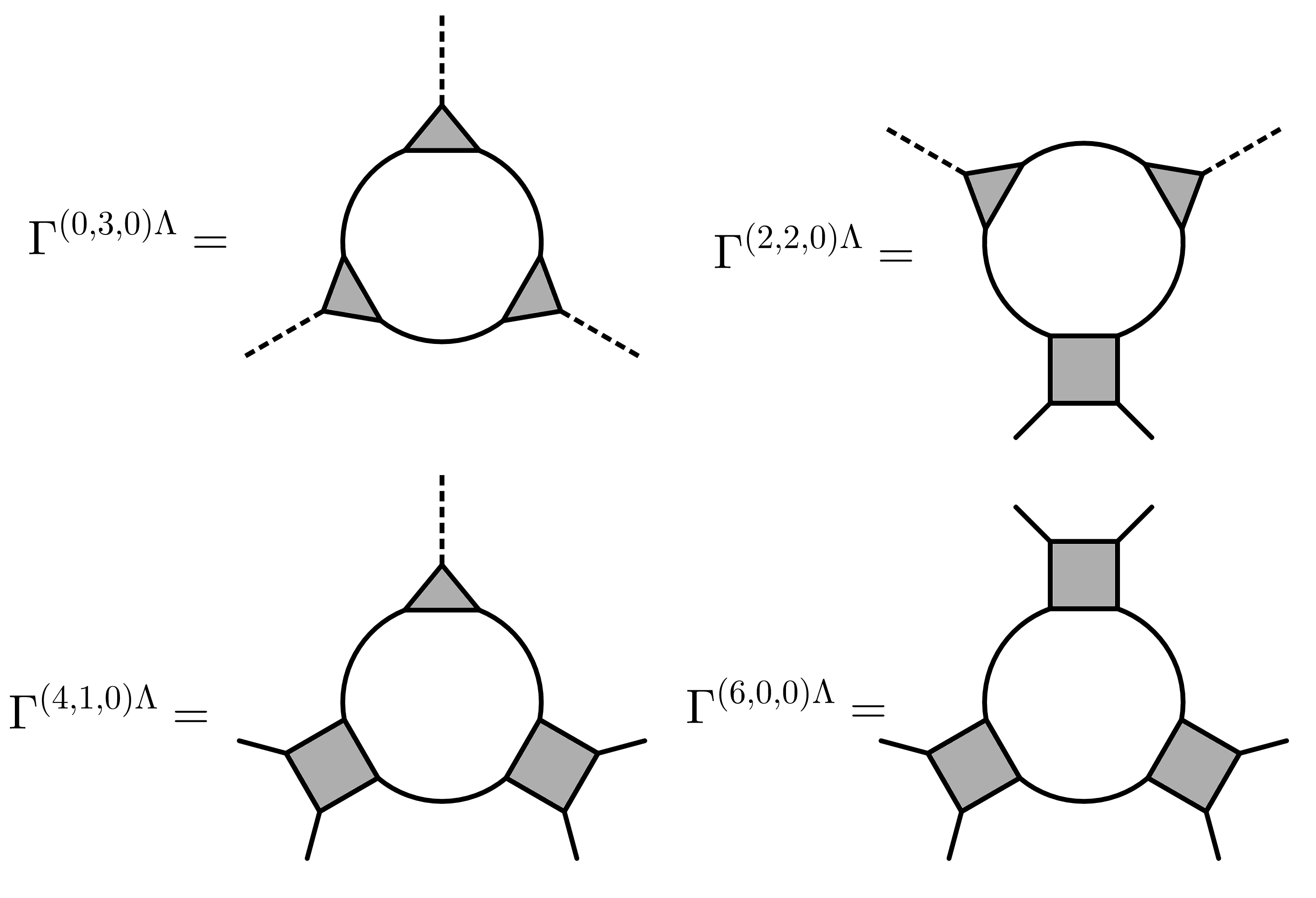
Figure 10: Feynman diagrams describing the Katanin-like approximation higher order correlation functions. The conventions are the same as in Figs. 1 and 2.

Appendix B Calculation of the irreducible vertex in the bosonic formalism

In this appendix we provide a proof of Eq. (47) by making use of matrix notation. If the full vertex can be decomposed as in Eq. (26)

$$V=\mathcal{Q}+\frac{h[h]^{T}}{m},$$ (91)

we can plug this relation into the definition of the irreducible vertex, Eq. (18). With some algebra we obtain

$$\begin{split}\widetilde{V}=&\left[1+V\Pi\right]^{-1}V=\\ =&\left[1+\frac{\widetilde{h}[h]^{T}}{m}\Pi\right]^{-1}\left[\widetilde{\mathcal{Q}}+\frac{\widetilde{h}[h]^{T}}{m}\right],\end{split}$$ (92)

where in the last line we have inserted a representation of the identity,

$$1=\left[1+\mathcal{Q}\Pi\right]\left[1+\mathcal{Q}\Pi\right]^{-1},$$ (93)

in between the two matrices and we have made use of definitions (38) and (40). With a bit of simple algebra, we can analytically invert the matrix on the left in the last line of Eq. (92), obtaining

$$\left[1+\frac{\widetilde{h}[h]^{T}}{m}\Pi\right]^{-1}=1-\frac{\widetilde{h}[h]^{T}}{\widetilde{m}}\Pi,$$ (94)

Where $\widetilde{m}$ is defined in Eq. (42). By plugging this result into Eq. (92), we finally obtain

$$\widetilde{V}=\widetilde{\mathcal{Q}}+\frac{\widetilde{h}[\widetilde{h}]^{T}}{\widetilde{m}},$$ (95)

that is the result of Eq. (47).

Appendix C Algorithm for the calculation of the superfluid gap

The formalism described in Sec. V allows us to formulate a minimal set of closed equations required for the calculation of the gap. We drop the $\Lambda$ superscript, assuming that we have reached the final scale. The gap can be computed using the Ward identity, so we can reduce ourselves to a single self consistent equation for $\alpha$, that is a single scalar quantity, and another one for $h_{\pi}$, momentum dependent. The equation for $\alpha$ is Eq. (50). The transverse Yukawa coupling is calculated through Eq. (44). The equations are coupled since the superfluid gap $\Delta=\alpha h_{\pi}$ appears in the r.h.s of both.
We propose an iterative loop to solve the above mentioned equations. By starting with the initial conditions $\alpha^{(0)}=0$ and $h_{\pi}^{(0)}(k)=0$, we update the transverse Yukawa coupling at every loop iteration $i$ according to Eq. (44), that can be reformulated in the following algorithmic form:

$$h_{\pi}^{(i+1)}(k)=\int_{k^{\prime}}\left[M^{(i)}(k,k^{\prime})\right]^{-1}\,\widetilde{h}^{\Lambda_{s}}(k^{\prime}),$$ (96)

with the matrix $M^{(i)}$ defined as

$$M^{(i)}(k,k^{\prime})=\delta_{k,k^{\prime}}-\mathcal{\widetilde{Q}}^{\Lambda_{s}}(k,k^{\prime})\,\Pi_{22}^{(i)}(k^{\prime};\alpha^{(i)}),$$ (97)

and the $22$-bubble rewritten as

$$\Pi_{22}^{(i)}(k;\alpha)=\frac{1}{G^{-1}(k)G^{-1}(-k)+\alpha^{2}\left[h_{\pi}^{(i)}(k)\right]^{2}},$$ (98)

with $G(k)$ defined in Eq. (17). Eq. (96) is not solved self consistently at every loop iteration $i$, because we have chosen to evaluate the r.h.s with $h_{\pi}$ at the previous iteration. $\alpha^{(i+1)}$ is calculated by self consistently solving

$$1=\frac{1}{\widetilde{m}^{\Lambda_{s}}}\int_{k}\widetilde{h}^{\Lambda_{s}}(k)\,\Pi_{22}^{(i+1)}(k;\alpha)\,h_{\pi}^{(i+1)}(k)$$ (99)

for $\alpha$. The equation above is nothing but Eq. (50) where the solution $\alpha=0$ has been factorized away. The loop consisting of Eqs. (96) and (99) must be repeated until convergence is reached in $\alpha$ and, subsequently, in $h_{\pi}$. This formulation of self consistent equations is not computationally lighter than the one in the fermionic formalism, but more easily controllable, as one can split the frequency and momentum dependence of the gap (through $h_{\pi}$) from the strength of the order ($\alpha$). Moreover, thanks to the fact that $h_{\pi}$ is updated with an explicit expression, namely Eq. (96), that is in general a well behaved function of $k$, the frequency and momentum dependence of the gap is assured to be under control.

Appendix D Flow equations in the symmetric phase

The flow equations for the three channels, $\mathcal{C}^{\Lambda}$, $\mathcal{M}^{\Lambda}$ and $\mathcal{P}^{\Lambda}$ in the symmetric phase are similar to those obtained in Ref. [55] for the repulsive Hubbard model. For the charge channel we have

$$\begin{split}\partial_{\Lambda}\mathcal{C}^{\Lambda}_{\nu\nu^{\prime}}(\mathbf{q},\Omega)=-\sum_{\omega}L^{c,\Lambda}_{\nu,\omega+\Omega}(\mathbf{q},\Omega)\left[\widetilde{\partial}_{\Lambda}\chi^{c,\Lambda}_{\omega}(\mathbf{q},\Omega)\right]L^{c,\Lambda}_{\omega\nu^{\prime}}(\mathbf{q},\Omega),\end{split}$$ (100)

where

$$\begin{split}L^{c,\Lambda}_{\nu\nu^{\prime}}(\mathbf{q},\Omega)=U-\mathcal{C}^{\Lambda}_{\nu\nu^{\prime}}(\mathbf{q},\Omega)+\vbox{\hbox{\scaleto[3ex]{\displaystyle\int}{8ex}}}_{\mkern-15.0mu\mathbf{p}}\Bigg{[}\frac{1}{2}\mathcal{C}^{\Lambda}_{\nu\nu^{\prime}}(\mathbf{p},\nu^{\prime}-\nu-\Omega)+\frac{3}{2}\mathcal{M}^{\Lambda}_{\nu\nu^{\prime}}(\mathbf{p},\nu^{\prime}-\nu-\Omega)-\mathcal{P}^{\Lambda}_{\nu,\nu+\Omega}(\mathbf{p},\nu+\nu^{\prime})\Bigg{]},\end{split}$$ (101)

and

$$\chi^{c,\Lambda}_{\nu}(\mathbf{q},\Omega)=T\int_{\mathbf{k}}G_{0}^{\Lambda}\left(\mathbf{k}+\mathbf{q},\nu+\Omega\right)G_{0}^{\Lambda}\left(\mathbf{k},\nu\right),$$ (102)

with $G_{0}^{\Lambda}(k)=\frac{1}{Q_{0}^{\Lambda}(k)}=\frac{\nu^{2}}{\nu^{2}+\Lambda^{2}}\frac{1}{i\nu-\xi_{\mathbf{k}}}$, and $\int_{\mathbf{k}}=\int\frac{d^{2}\mathbf{k}}{(2\pi)^{2}}$. Similarly, the flow equation for the magnetic channel is given by

$$\begin{split}\partial_{\Lambda}\mathcal{M}^{\Lambda}_{\nu\nu^{\prime}}(\mathbf{q},\Omega)=-\sum_{\omega}L^{m,\Lambda}_{\nu,\omega+\Omega}(\mathbf{q},\Omega)\left[\widetilde{\partial}_{\Lambda}\chi^{m,\Lambda}_{\omega}(\mathbf{q},\Omega)\right]L^{m,\Lambda}_{\omega\nu^{\prime}}(\mathbf{q},\Omega),\end{split}$$ (103)

with $\chi^{m,\Lambda}_{\omega}(\mathbf{q},\Omega)=\chi^{c,\Lambda}_{\omega}(\mathbf{q},\Omega)$, and

$$\begin{split}L^{m,\Lambda}_{\nu\nu^{\prime}}(\mathbf{q},\Omega)=-U-\mathcal{M}^{\Lambda}_{\nu\nu^{\prime}}(\mathbf{q},\Omega)+\vbox{\hbox{\scaleto[3ex]{\displaystyle\int}{8ex}}}_{\mkern-15.0mu\mathbf{p}}\Bigg{[}\frac{1}{2}\mathcal{C}^{\Lambda}_{\nu\nu^{\prime}}(\mathbf{p},\nu^{\prime}-\nu-\Omega)-\frac{1}{2}\mathcal{M}^{\Lambda}_{\nu\nu^{\prime}}(\mathbf{p},\nu^{\prime}-\nu-\Omega)+\mathcal{P}^{\Lambda}_{\nu,\nu+\Omega}(\mathbf{p},\nu+\nu^{\prime})\Bigg{]}.\end{split}$$ (104)

Finally, the flow equation for the pairing channel reads

$$\begin{split}\partial_{\Lambda}\mathcal{P}^{\Lambda}_{\nu\nu^{\prime}}(\mathbf{q},\Omega)=\sum_{\omega}L^{p,\Lambda}_{\nu\omega}(\mathbf{q},\Omega)\left[\widetilde{\partial}_{\Lambda}\chi^{p,\Lambda}_{\omega}(\mathbf{q},\Omega)\right]L^{p,\Lambda}_{\omega\nu^{\prime}}(\mathbf{q},\Omega),\end{split}$$ (105)

where we have projected onto the singlet component of the pairing, that is

$$L^{p,\Lambda}_{\nu\nu^{\prime}}(\mathbf{q},\Omega)=\frac{\overline{L}^{p,\Lambda}_{\nu\nu^{\prime}}(\mathbf{q},\Omega)+\overline{L}^{p,\Lambda}_{\nu,\Omega-\nu^{\prime}}(\mathbf{q},\Omega)}{2},$$ (106)

with

$$\begin{split}\overline{L}^{p,\Lambda}_{\nu\nu^{\prime}}(\mathbf{q},\Omega)=-U+\mathcal{P}^{\Lambda}_{\nu\nu^{\prime}}(\mathbf{q},\Omega)+\vbox{\hbox{\scaleto[3ex]{\displaystyle\int}{8ex}}}_{\mkern-15.0mu\mathbf{p}}\Bigg{[}\frac{1}{2}\mathcal{C}^{\Lambda}_{\nu,\Omega-\nu}(\mathbf{p},\nu^{\prime}-\nu)-\frac{1}{2}\mathcal{M}^{\Lambda}_{\nu,\Omega-\nu}(\mathbf{p},\nu^{\prime}-\nu)-\mathcal{M}^{\Lambda}_{\nu,\Omega-\nu}(\mathbf{p},\Omega-\nu-\nu^{\prime})\Bigg{]},\end{split}$$ (107)

and

$$\chi^{p,\Lambda}_{\nu}(\mathbf{q},\Omega)=T\int_{\mathbf{k}}G_{0}^{\Lambda}\left(\mathbf{k},\nu\right)G_{0}^{\Lambda}\left(\mathbf{q}-\mathbf{k},\Omega-\nu\right).$$ (108)

References

- Eagles [1969] D. M. Eagles, Possible Pairing without Superconductivity at Low Carrier Concentrations in Bulk and Thin-Film Superconducting Semiconductors, Phys. Rev. 186, 456 (1969).
- Leggett [1980] A. J. Leggett, Diatomic Molecules and Cooper Pairs (1980), in Modern Trends in the Theory of Condensed Matter, edited by A. Pekalski and J. A. Przystawa (Springer, Berlin, 1980).
- Nozières and Schmitt-Rink [1985] P. Nozières and S. Schmitt-Rink, Bose condensation in an attractive fermion gas: From weak to strong coupling superconductivity, J. Low Temp. Phys. 59, 195 (1985).
- Mermin and Wagner [1966] N. D. Mermin and H. Wagner, Absence of Ferromagnetism or Antiferromagnetism in One- or Two-Dimensional Isotropic Heisenberg Models, Phys. Rev. Lett. 17, 1133 (1966).
- Hohenberg [1967] P. C. Hohenberg, Existence of Long-Range Order in One and Two Dimensions, Phys. Rev. 158, 383 (1967).
- Berezinskii [1971] V. L. Berezinskii, Destruction of Long-range Order in One-dimensional and Two-dimensional Systems having a Continuous Symmetry Group I. Classical Systems, Sov. Phys. JETP 32, 493 (1971).
- Kosterlitz and Thouless [1973] J. M. Kosterlitz and D. J. Thouless, Ordering, metastability and phase transitions in two-dimensional systems, J. Phys. C 6, 1181 (1973).
- Metzner et al. [2012] W. Metzner, M. Salmhofer, C. Honerkamp, V. Meden, and K. Schönhammer, Functional renormalization group approach to correlated fermion systems, Rev. Mod. Phys. 84, 299 (2012).
- Kopietz and Schütz [2010] L. Kopietz, P. Bartosch and F. Schütz, Introduction to the Functional Renormalization Group (Springer, Berlin, 2010).
- Zanchi and Schulz [2000] D. Zanchi and H. J. Schulz, Weakly correlated electrons on a square lattice: Renormalization-group theory, Phys. Rev. B 61, 13609 (2000).
- Halboth and Metzner [2000] C. J. Halboth and W. Metzner, Renormalization-group analysis of the two-dimensional Hubbard model, Phys. Rev. B 61, 7364 (2000).
- Honerkamp et al. [2001] C. Honerkamp, M. Salmhofer, N. Furukawa, and T. M. Rice, Breakdown of the Landau-Fermi liquid in two dimensions due to umklapp scattering, Phys. Rev. B 63, 035109 (2001).
- Freire et al. [2008] H. Freire, E. Correa, and A. Ferraz, Breakdown of the Fermi-liquid regime in the two-dimensional Hubbard model from a two-loop field-theoretical renormalization group approach, Phys. Rev. B 78, 125114 (2008).
- Eberlein [2014] A. Eberlein, Fermionic two-loop functional renormalization group for correlated fermions: Method and application to the attractive Hubbard model, Phys. Rev. B 90, 115125 (2014).
- Hille et al. [2020] C. Hille, F. B. Kugler, C. J. Eckhardt, Y.-Y. He, A. Kauch, C. Honerkamp, A. Toschi, and S. Andergassen, Quantitative functional renormalization group description of the two-dimensional Hubbard model, Phys. Rev. Research 2, 033372 (2020).
- Schütz et al. [2005] F. Schütz, L. Bartosch, and P. Kopietz, Collective fields in the functional renormalization group for fermions, Ward identities, and the exact solution of the Tomonaga-Luttinger model, Phys. Rev. B 72, 035107 (2005).
- Bartosch et al. [2009a] L. Bartosch, H. Freire, J. J. R. Cardenas, and P. Kopietz, A functional renormalization group approach to the anderson impurity model, J. Phys. Condens. Matter 21, 305602 (2009a).
- Isidori et al. [2010] A. Isidori, D. Roosen, L. Bartosch, W. Hofstetter, and P. Kopietz, Spectral function of the Anderson impurity model at finite temperatures, Phys. Rev. B 81, 235120 (2010).
- Streib et al. [2013] S. Streib, A. Isidori, and P. Kopietz, Solution of the Anderson impurity model via the functional renormalization group, Phys. Rev. B 87, 201107(R) (2013).
- Lange et al. [2015] P. Lange, C. Drukier, A. Sharma, and P. Kopietz, Summing parquet diagrams using the functional renormalization group: X-ray problem revisited, J. Phys. A 48, 395001 (2015).
- Lange et al. [2017] P. Lange, O. Tsyplyatyev, and P. Kopietz, Critical pairing fluctuations in the normal state of a superconductor: Pseudogap and quasiparticle damping, Phys. Rev. B 96, 064506 (2017).
- Diehl et al. [2007a] S. Diehl, H. Gies, J. M. Pawlowski, and C. Wetterich, Flow equations for the BCS-BEC crossover, Phys. Rev. A 76, 021602(R) (2007a).
- Diehl et al. [2007b] S. Diehl, H. Gies, J. M. Pawlowski, and C. Wetterich, Renormalization flow and universality for ultracold fermionic atoms, Phys. Rev. A 76, 053627 (2007b).
- Strack et al. [2008] P. Strack, R. Gersch, and W. Metzner, Renormalization group flow for fermionic superfluids at zero temperature, Phys. Rev. B 78, 014522 (2008).
- Bartosch et al. [2009b] L. Bartosch, P. Kopietz, and A. Ferraz, Renormalization of the BCS-BEC crossover by order-parameter fluctuations, Phys. Rev. B 80, 104514 (2009b).
- Obert et al. [2013] B. Obert, C. Husemann, and W. Metzner, Low-energy singularities in the ground state of fermionic superfluids, Phys. Rev. B 88, 144508 (2013).
- Schütz and Kopietz [2006] F. Schütz and P. Kopietz, Functional renormalization group with vacuum expectation values and spontaneous symmetry breaking, J. Phys. A 39, 8205 (2006).
- Baier et al. [2004] T. Baier, E. Bick, and C. Wetterich, Temperature dependence of antiferromagnetic order in the Hubbard model, Phys. Rev. B 70, 125111 (2004).
- Floerchinger et al. [2008] S. Floerchinger, M. Scherer, S. Diehl, and C. Wetterich, Particle-hole fluctuations in BCS-BEC crossover, Phys. Rev. B 78, 174528 (2008).
- Krahl et al. [2009] H. C. Krahl, J. A. Müller, and C. Wetterich, Generation of -wave coupling in the two-dimensional Hubbard model from functional renormalization, Phys. Rev. B 79, 094526 (2009).
- Friederich et al. [2010] S. Friederich, H. C. Krahl, and C. Wetterich, Four-point vertex in the Hubbard model and partial bosonization, Phys. Rev. B 81, 235108 (2010).
- Friederich et al. [2011] S. Friederich, H. C. Krahl, and C. Wetterich, Functional renormalization for spontaneous symmetry breaking in the Hubbard model, Phys. Rev. B 83, 155125 (2011).
- Salmhofer et al. [2004] M. Salmhofer, C. Honerkamp, W. Metzner, and O. Lauscher, Renormalization Group Flows into Phases with Broken Symmetry, Prog. Theor. Phys. 112, 943 (2004).
- Gersch et al. [2008] R. Gersch, C. Honerkamp, and W. Metzner, Superconductivity in the attractive Hubbard model: functional renormalization group analysis, New J. Phys. 10, 045003 (2008).
- Eberlein and Metzner [2013] A. Eberlein and W. Metzner, Effective interactions and fluctuation effects in spin-singlet superfluids, Phys. Rev. B 87, 174523 (2013).
- Eberlein and Metzner [2014] A. Eberlein and W. Metzner, Superconductivity in the two-dimensional --Hubbard model, Phys. Rev. B 89, 035126 (2014).
- Maier et al. [2014] S. A. Maier, A. Eberlein, and C. Honerkamp, Functional renormalization group for commensurate antiferromagnets: Beyond the mean-field picture, Phys. Rev. B 90, 035140 (2014).
- Gersch et al. [2005] R. Gersch, C. Honerkamp, D. Rohe, and W. Metzner, Fermionic renormalization group flow into phases with broken discrete symmetry: charge-density wave mean-field model, Eur. Phys. J. B 48, 349 (2005).
- Wang et al. [2014] J. Wang, A. Eberlein, and W. Metzner, Competing order in correlated electron systems made simple: Consistent fusion of functional renormalization and mean-field theory, Phys. Rev. B 89, 121116(R) (2014).
- Yamase et al. [2016] H. Yamase, A. Eberlein, and W. Metzner, Coexistence of Incommensurate Magnetism and Superconductivity in the Two-Dimensional Hubbard Model, Phys. Rev. Lett. 116, 096402 (2016).
- Kugler and von Delft [2018a] F. B. Kugler and J. von Delft, Multiloop Functional Renormalization Group That Sums Up All Parquet Diagrams, Phys. Rev. Lett. 120, 057403 (2018a).
- Kugler and von Delft [2018b] F. B. Kugler and J. von Delft, Multiloop functional renormalization group for general models, Phys. Rev. B 97, 035162 (2018b).
- Tagliavini et al. [2019] A. Tagliavini, C. Hille, F. B. Kugler, S. Andergassen, A. Toschi, and C. Honerkamp, Multiloop functional renormalization group for the two-dimensional Hubbard model: Loop convergence of the response functions, SciPost Phys. 6, 9 (2019).
- Georges et al. [1996] A. Georges, G. Kotliar, W. Krauth, and M. J. Rozenberg, Dynamical mean-field theory of strongly correlated fermion systems and the limit of infinite dimensions, Rev. Mod. Phys. 68, 13 (1996).
- Taranto et al. [2014] C. Taranto, S. Andergassen, J. Bauer, K. Held, A. Katanin, W. Metzner, G. Rohringer, and A. Toschi, From Infinite to Two Dimensions through the Functional Renormalization Group, Phys. Rev. Lett. 112, 196402 (2014).
- Vilardi et al. [2019] D. Vilardi, C. Taranto, and W. Metzner, Antiferromagnetic and -wave pairing correlations in the strongly interacting two-dimensional Hubbard model from the functional renormalization group, Phys. Rev. B 99, 104501 (2019).
- Denz et al. [2020] T. Denz, M. Mitter, J. M. Pawlowski, C. Wetterich, and M. Yamada, Partial bosonization for the two-dimensional Hubbard model, Phys. Rev. B 101, 155115 (2020).
- Krien et al. [2019] F. Krien, A. Valli, and M. Capone, Single-boson exchange decomposition of the vertex function, Phys. Rev. B 100, 155149 (2019).
- Krien and Valli [2019] F. Krien and A. Valli, Parquetlike equations for the Hedin three-leg vertex, Phys. Rev. B 100, 245147 (2019).
- Ayral and Parcollet [2016] T. Ayral and O. Parcollet, Mott physics and spin fluctuations: A functional viewpoint, Phys. Rev. B 93, 235124 (2016).
- Rubtsov et al. [2012] A. Rubtsov, M. Katsnelson, and A. Lichtenstein, Dual boson approach to collective excitations in correlated fermionic systems, Ann. Phys. 327, 1320 (2012).
- Stepanov et al. [2018] E. A. Stepanov, S. Brener, F. Krien, M. Harland, A. I. Lichtenstein, and M. I. Katsnelson, Effective Heisenberg Model and Exchange Interaction for Strongly Correlated Systems, Phys. Rev. Lett. 121, 037204 (2018).
- Stepanov et al. [2019] E. A. Stepanov, V. Harkov, and A. I. Lichtenstein, Consistent partial bosonization of the extended Hubbard model, Phys. Rev. B 100, 205115 (2019).
- Peters et al. [2019] L. Peters, E. G. C. P. van Loon, A. N. Rubtsov, A. I. Lichtenstein, M. I. Katsnelson, and E. A. Stepanov, Dual boson approach with instantaneous interaction, Phys. Rev. B 100, 165128 (2019).
- Vilardi et al. [2017] D. Vilardi, C. Taranto, and W. Metzner, Nonseparable frequency dependence of the two-particle vertex in interacting fermion systems, Phys. Rev. B 96, 235110 (2017).
- Wetterich [1993] C. Wetterich, Exact evolution equation for the effective potential, Phys. Lett. B 301, 90 (1993).
- Berges et al. [2002] J. Berges, N. Tetradis, and C. Wetterich, Non-perturbative renormalization flow in quantum field theory and statistical physics, Phys. Rep. 363, 223 (2002).
- Randeria et al. [1992] M. Randeria, N. Trivedi, A. Moreo, and R. T. Scalettar, Pairing and spin gap in the normal state of short coherence length superconductors, Phys. Rev. Lett. 69, 2001 (1992).
- dos Santos [1994] R. R. dos Santos, Spin gap and superconductivity in the three-dimensional attractive Hubbard model, Phys. Rev. B 50, 635 (1994).
- Trivedi and Randeria [1995] N. Trivedi and M. Randeria, Deviations from Fermi-Liquid Behavior above in 2D Short Coherence Length Superconductors, Phys. Rev. Lett. 75, 312 (1995).
- Singer et al. [1996] J. M. Singer, M. H. Pedersen, T. Schneider, H. Beck, and H.-G. Matuttis, From BCS-like superconductivity to condensation of local pairs: A numerical study of the attractive Hubbard model, Phys. Rev. B 54, 1286 (1996).
- Karakuzu et al. [2018] S. Karakuzu, K. Seki, and S. Sorella, Study of the superconducting order parameter in the two-dimensional negative- Hubbard model by grand-canonical twist-averaged boundary conditions, Phys. Rev. B 98, 075156 (2018).
- Keller et al. [2001] M. Keller, W. Metzner, and U. Schollwöck, Dynamical Mean-Field Theory for Pairing and Spin Gap in the Attractive Hubbard Model, Phys. Rev. Lett. 86, 4612 (2001).
- Capone et al. [2002] M. Capone, C. Castellani, and M. Grilli, First-Order Pairing Transition and Single-Particle Spectral Function in the Attractive Hubbard Model, Phys. Rev. Lett. 88, 126403 (2002).
- Toschi et al. [2005] A. Toschi, M. Capone, and C. Castellani, Energetic balance of the superconducting transition across the BCS—Bose Einstein crossover in the attractive Hubbard model, Phys. Rev. B 72, 235118 (2005).
- Del Re et al. [2019] L. Del Re, M. Capone, and A. Toschi, Dynamical vertex approximation for the attractive hubbard model, Phys. Rev. B 99, 045137 (2019).
- Eberlein [2013] A. Eberlein, Functional renormalization group study of fluctuation effects in fermionic superfluids, Ph.D. thesis, University of Stuttgart (2013).
- Katanin [2004] A. A. Katanin, Fulfillment of Ward identities in the functional renormalization group approach, Phys. Rev. B 70, 115109 (2004).
- [69] One can prove it by considering the effective interaction functional , as shown in Ref. [8].
- Husemann and Salmhofer [2009] C. Husemann and M. Salmhofer, Efficient parametrization of the vertex function, scheme, and the Hubbard model at van Hove filling, Phys. Rev. B 79, 195125 (2009).
- Husemann et al. [2012] C. Husemann, K.-U. Giering, and M. Salmhofer, Frequency-dependent vertex functions of the () Hubbard model at weak coupling, Phys. Rev. B 85, 075121 (2012).
- Lichtenstein et al. [2017] J. Lichtenstein, D. Sánchez de la Peña, D. Rohe, E. Di Napoli, C. Honerkamp, and S. A. Maier, High-performance functional Renormalization Group calculations for interacting fermions, Comput. Phys. Commun. 213, 100 (2017).
- Wentzell et al. [2020] N. Wentzell, G. Li, A. Tagliavini, C. Taranto, G. Rohringer, K. Held, A. Toschi, and S. Andergassen, High-frequency asymptotics of the vertex function: Diagrammatic parametrization and algorithmic implementation, Phys. Rev. B 102, 085106 (2020).
- van Loon et al. [2018] E. G. C. P. van Loon, F. Krien, H. Hafermann, A. I. Lichtenstein, and M. I. Katsnelson, Fermion-boson vertex within dynamical mean-field theory, Phys. Rev. B 98, 205148 (2018).
- Rohringer et al. [2012] G. Rohringer, A. Valli, and A. Toschi, Local electronic correlation at the two-particle level, Phys. Rev. B 86, 125114 (2012).
- Micnas et al. [1990] R. Micnas, J. Ranninger, and S. Robaszkiewicz, Superconductivity in narrow-band systems with local nonretarded attractive interactions, Rev. Mod. Phys. 62, 113 (1990).
- Gor’kov and Melik-Barkhudarov [1961] L. P. Gor’kov and T. K. Melik-Barkhudarov, Contribution to the Theory of Superfluidity in an Imperfect Fermi Gas, Sov. Phys. JETP 13, 1018 (1961).
- Anderson [1952] P. W. Anderson, An Approximate Quantum Theory of the Antiferromagnetic Ground State, Phys. Rev. 86, 694 (1952).
- Bonetti et al. [2020] P. M. Bonetti, J. Mitscherling, D. Vilardi, and W. Metzner, Charge carrier drop at the onset of pseudogap behavior in the two-dimensional Hubbard model, Phys. Rev. B 101, 165142 (2020).